Context Tree based Image Contour Coding using A Geometric Prior
Abstract
If object contours in images are coded efficiently as side information, then they can facilitate advanced image / video coding techniques, such as graph Fourier transform coding or motion prediction of arbitrarily shaped pixel blocks. In this paper, we study the problem of lossless and lossy compression of detected contours in images. Specifically, we first convert a detected object contour composed of contiguous between-pixel edges to a sequence of directional symbols drawn from a small alphabet. To encode the symbol sequence using arithmetic coding, we compute an optimal variable-length context tree (VCT) via a maximum a posterior (MAP) formulation to estimate symbols’ conditional probabilities. MAP prevents us from overfitting given a small training set of past symbol sequences by identifying a VCT that achieves a high likelihood of observing given , and a large geometric prior stating that image contours are more often straight than curvy. For the lossy case, we design efficient dynamic programming (DP) algorithms that optimally trade off coding rate of an approximate contour given a VCT with two notions of distortion of with respect to the original contour . To reduce the size of the DP tables, a total suffix tree is derived from a given VCT for compact table entry indexing, reducing complexity. Experimental results show that for lossless contour coding, our proposed algorithm outperforms state-of-the-art context-based schemes consistently for both small and large training datasets. For lossy contour coding, our algorithms outperform comparable schemes in the literature in rate-distortion performance.
Index Terms:
contour coding, lossless coding, statistical learning, image compressionI Introduction
Advances in depth sensing technologies like Microsoft Kinect 2.0 mean that depth images—per pixel distances between physical objects in a 3D scene and the camera—can now be captured easily and inexpensively. Depth imaging has in turn eased the detection of object contours in a captured image, which was traditionally a challenging computer vision problem [1]. If detected object contours in images are compressed efficiently as side information (SI), then they can enable advanced image / video coding techniques such as graph Fourier transform (GFT) coding [2, 3, 4, 5] and motion prediction [6, 7] of arbitrarily shaped pixel blocks. Moreover, coded contours can be transmitted to a central cloud for computation-intensive object detection or activity recognition [8], at a much lower coding cost than compressed depth video. We focus on the problem of coding object contours in this paper.
Object contour coding was studied extensively during 1990’s when the concept of object-based video coding (OBVC) was popular during the MPEG-4 video coding standardization. However, the shape coding techniques developed to represent boundaries of objects [9]—called video object planes (VOP)—were not efficient enough, resulting in large SI overhead that rendered OBVC uncompetitive in compression performance. Some contemporary interest in the problem has shifted to lossy contour coding, where curve- and spline-based approximations are used [10, 11, 12].
Two recent technological trends have provided new ammunitions to revisit the old lossless contour coding problem. First, advances in statistical machine learning have led to sophisticated algorithms that construct suitable variable-length context trees (VCT) to estimate conditional probabilities given a training dataset of symbol strings [13, 14, 15, 16]. Estimated probability distributions can then be used to compress symbol strings of finite alphabets via arithmetic coding [17]. Second, the availability of fast computing resource, locally or in a nearby cloudlet [18], allows this statistical learning on relevant training datasets to be performed in real-time in restricted cases. While promising, the convergence of these developments has led to a new “small data” statistical learning problem: due to either statistical non-stationarity and/or tight real-time application requirements, the size of dataset used for statistical training may be limited, and data overfitting becomes a significant concern.
In response, in this paper we propose a maximum a posteriori (MAP) formulation to optimize a VCT for lossless and lossy contour coding. In particular, given small training data , we select a VCT that has both high likelihood (agreement between constructed contexts and observations), and high prior probability —a geometric prior stating that image contours are more often straight than curvy. Like Bayesian information criterion (BIC) [19], we design the prior weight parameter to scale naturally with training data size, so that when the volume of relevant training data becomes larger and thus more reliable, becomes smaller.
For lossy coding, we design efficient dynamic programming (DP) algorithms that optimally trade off coding rate of an approximate contour given a VCT with two different notions of distortion of with respect to the original contour : sum squared distance distortion (SSDD) and maximum absolute distance distortion (MADD) [9]. To reduce the size of the DP tables, a new tool called total suffix tree (TST) is derived from a VCT for compact table entry indexing, reducing computation complexity. Experimental results show that for lossless contour coding, our proposed algorithm outperforms state-of-the-art context-based schemes [13, 7] consistently for both small and large training datasets. For lossy contour coding, our algorithms outperform comparable schemes in the literature [9, 12] in rate-distortion (RD) performance. Towards the goal of reproducible research [20], we have made the source code for lossless contour coding publicly available111http://research.nii.ac.jp/~cheung/software.html.
The outline of the paper is as follows. We first discuss related works in Section II. We then discuss our proposal for lossless and lossy contour coding in Section III and IV, respectively. We discuss efficient coding of contour starting points in Section V. Finally, we present experimental results and conclusion in Section VI and VII, respectively.
II Related Work
II-A Lossless Contour Coding
Most works in lossless contour coding [7, 21, 22, 17, 23, 24, 25, 26, 27] first convert an image contour into a chain code [28]: a sequence of symbols each representing one of four or eight possible absolute directions on the pixel grid. Alternatively, a differential chain code (DCC) [21] that specifies relative directions instead can be used. DCC symbols are entropy-coded using either Huffman [22] or arithmetic coding [17] given symbol probabilities. The challenge is to estimate conditional probabilities for DCC symbols given a set of training data; this is the core problem we address in Section III.
[29, 7] propose a linear geometric model to estimate conditional probabilities of the next DCC symbol. In summary, given a window of previous edges, a line-of-best-fit that minimizes the sum of distances to the edges’ endpoints is first constructed. Then the probability of a candidate direction for the next symbol is assumed inversely proportional to the angle difference between the direction and the fitted line. We show in Section VI that this scheme is inferior in estimating symbol probabilities compared to context models, because there are only a few possible angle differences for a small number of previous edges, limiting the expressiveness of the model.
An alternative approach is context modeling: given a window of previous symbols (context) , compute the conditional probability of the next symbol by counting the number of occurrences of followed by in the training data. In [30, 17, 23, 24, 25], Markov models of fixed order up to eight are used for lossless coding. However, in applications where the training data is small, there may be not enough occurrences of to reliably estimate the conditional probabilities.
VCT [14, 13] provides a more flexible approach for Markov context modeling by allowing the context to have variable length. There are many ways to construct the VCT: Lempel-Ziv-78 (LZ78) [31], prediction by partial matching (PPM) [15], and probabilistic suffix trees (PST) [16]. LZ78 constructs a dictionary from scratch using the input data directly as training data. The probability estimation quality varies depending on the order of first appearing input symbols. PPM considers all contexts restricted by a maximum length with non-zero occurrences in the training data when building VCT. PPM is efficient for lossless sequential data compression if sufficient training data is available [26, 27], but may suffer from overfitting if training data is limited.
PST first constructs an initial VCT similar to PPM, and then the initial VCT is pruned using five user-selected thresholds [16]. PST algorithm is widely used for protein modeling problems [32, 33]. Through pruning, PST algorithm can avoid overfitting in some cases. However, choosing properly the five application-specific thresholds used for pruning is difficult in general. In contrast, we propose a geometric shape prior—requiring only one parameter—to avoid overfitting specifically for contour coding.
II-B Lossy Contour Coding
There are two main approaches to lossy contour coding: chain-code-based and vertex-based. In the first approach, the contours are first converted to chain codes as done in the lossless case. Then the chain codes are approximated according to different criteria before entropy coding. In [34], an approximated chain code must be composed of several predefined sub-chain codes, and the indices of the sub-chain codes are coded. In [35], a line processing technique generates straighter contour segments than the input, which are then efficiently compressed. In [7], a chain code is simplified by removing “irregularities”, which are predefined non-smooth edge patterns. All these approaches approximate the chain codes without considering explicitly distortion due to approximation, and one cannot specify a desired compression ratio. In contrast, we approximate a chain code via RD optimization algorithms, so that different compression ratios can be achieved.
Vertex-based approaches select representative points called vertices along the contour for coding. [36, 37] use a top-down / bottom-up framework to select and code vertices independently. [38, 39, 9] propose an operational rate-distortion (ORD) optimal algorithm to jointly select and code vertices. Many improvements on ORD have since been proposed, including [40, 41, 10, 11, 12]. Compared to the chain-code-based approach, the vertex-based approach requires fewer points for coding, but each point (vertex) will consume more bits. We follow the chain-code-based approach for lossy coding in Section IV.
III Lossless Contour Coding
We first propose an algorithm to efficiently code object contours losslessly in a target image. A small set of training images are used for statistical learning; we assume that the target image and the training images are statistically correlated, such as consecutive frames in a video sequence. We assume also that, as a pre-processing step, object contours in an image have first been either outlined manually, or detected automatically using an existing method such as gradient-based edge detection [7]. Each contour is defined by a starting point and a sequence of connected edges. See Fig. 1 for two example contours of VOPs in a frame of MPEG4 test sequence news222ftp://ftp.tnt.uni-hannover.de/pub/MPEG/mpeg4_masks/. Our objective here is to losslessly encode the sequence of connected edges in a given contour; coding of the starting points of contours is discussed later in Section V.
We first overview our lossless contour coding algorithm, based on the general concept of context tree model [14, 13]. The algorithm is composed of the following steps:
-
1)
Convert each contour in a set of training images and a target image into a differential chain code (DCC) [21]—a string of symbols each chosen from a size-three alphabet.
-
2)
Construct a suitable context tree given the DCC strings in the training images by solving a maximum a posterior (MAP) problem.
-
3)
For each symbol in an input DCC string (corresponding to a contour in the target image), identify the conditional probability distribution using the constructed context tree, which is used for arithmetic coding of the symbol.
We discuss these steps in order. Notations for the technical discussions in the sequel are shown in Table I.
| Notation | Description |
|---|---|
| alphabet of relative directions, | |
| alphabet of absolute directions, | |
| training set of DCC strings | |
| -th DCC string in training set | |
| number of DCC strings in | |
| number of symbols in string | |
| total number of symbols in | |
| number of occurrences of sub-string in | |
| conditional probability of symbol given context | |
| DCC string and its -th symbol, | |
| length of the DCC string | |
| approximated DCC string | |
| length of the approximated DCC string | |
| A sub-string of length from to , | |
| context | |
| context tree, an optimal context tree | |
| context forest composed of all possible context trees | |
| maximum depth of the context tree | |
| initial context tree | |
| Number of nodes on | |
| total suffix tree | |
| prior weight parameter, | |
| maximum distortion of the approximated DCC string |
III-A Differential Chain Code
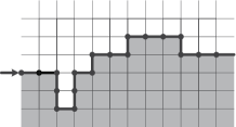
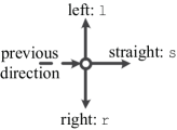
We first convert each contour into a DCC string; DCC is one member of the family of chain codes proposed by Freeman [21]. A contour is composed of a sequence of “between-pixel” edges that divide pixels in the local neighborhood into two sides, as illustrated in Fig. 2(a). A length- contour can be compactly described as a symbol string denoted by . For the first edge , we assume equal probability for each of four absolute directions, north, east, south and west, with respect to the starting point. For each subsequent DCC symbol , , only three relative directions are possible on a 2D grid with respect to the previous symbol : left, straight and right, as shown in Fig. 2(b). We denote them by l, s and r, respectively, which constitute a size-three alphabet . The problem is thus to code a DCC string (without the first edge), where for .

(a)

(b)
(a)
(b)
III-B Definition of Context Tree
We first define notations. Denote by , , the -th DCC string in the training set , where denotes the total number of DCC strings in . The length of is denoted by , and the total number of symbols in is denoted by .
Denote by , and , a sub-string of length from the -th symbol to the -th symbol in reverse order. Further, denote by the concatenation of sub-strings and .
We now define as the number of occurrences of sub-string in the training set . can be computed as:
| (1) |
where is an indicator function that evaluates to if the specified binary clause is true and otherwise.
Denote by the conditional probability of symbol occurring given its previous sub-string is , where . Given training data , can be estimated using as done in [32],
| (2) |
Given , we learn a context model to assign a conditional probability to any symbol given its previous symbols in a DCC string. Specifically, to calculate the conditional probability for the symbol given all its previous symbols , the model determines a context to calculate , where is a prefix of the sub-string , i.e., for some context length :
| (3) |
is calculated using (2) given . The context model determines a unique context of finite length for every possible past . The set of all mappings from to can be represented compactly as a context tree.
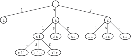
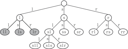
Denote by the context tree, where is a full ternary tree: each node has either zero children (an end node) or all three children (an intermediate node). The root node has an empty sub-string, and each child node has a sub-string that is a concatenation of: i) its parent’s sub-string if any, and ii) the symbol (one of l, s and r) representing the link connecting the parent node and itself in . An example is shown in Fig. 3. The sub-strings of the end nodes are the contexts of the tree . For each , a context is obtained by traversing from the root node until an end node, matching symbols into the past.
All possible context trees constitute a context forest denoted by . The modeling problem is to find the best tree from the forest given .
III-C Problem Definition for Optimal Context Tree
Given limited observations , we aim to find a suitable tree that best describes without overfitting. We first write the posterior probability of given via Bayes’ rule:
| (4) |
where is the likelihood of observing given context tree , and is the prior which describes a priori knowledge about the context tree. We next define the likelihood and prior terms, and then use the MAP estimator to formulate the context tree optimization problem.
III-C1 Likelihood Term
The likelihood is defined as the joint conditional probability of all the observed symbols in given their past and ,
| (5) |
Given tree , for each symbol a prefix (context) of past symbols is identified to compute the conditional probability. Hence (5) can be rewritten as follows using (3), similarly done in [42]:
| (6) |
III-C2 Prior Term
Overfitting occurs if the complexity of a model is too large for the given observed data size. In the case of context tree, it means that the number of occurrences of a particular context is too small to have probabilities reliably estimated using . To avoid overfitting, one can design a prior to control the size of —the complexity of the model—depending on the volume of training data. This general idea is used for example in [42], where Bayesian information criterion (BIC) [19] is employed to constrain the order of a fixed-length Markov model for given data size.
In the case of contour coding, we propose a geometric prior, defined as the sum of straightness, , of all contexts in tree , based on the assumption that contours in natural images are more likely straight than curvy. We calculate as follows. We first map a context to a shape segment on a 2D grid with points from the most recent symbol to the symbol furthest in the past plus an initial edge. Without loss of generality, we assume that the absolute direction of the initial edge is East. As an example, Fig. 4(b) shows a context with five points, where the dotted arrow is the initial edge. Denote by , , the 2D coordinate of the -th point. is defined as the maximum distance from any to a straight line connecting and ,
| (7) |
Some examples of are shown in Fig. 4.

(a)

(b)

(c)
We can now define prior based on the sum of of all contexts in as follows:
| (8) |
where is an important parameter to be discussed soon. We see that in general a tree with fewer contexts has a smaller sum in (8), meaning that our prior tends to reduce the number of parameters. Further, in general fewer contexts also means a shallower context tree. Thus, our prior promotes shorter contexts, which is also reasonable.
III-C3 MAP Estimation
We can now write the optimal context tree problem via a MAP formulation:
| (9) |
(9) can be rewritten as:
| (10) |
For ease of computation, we minimize the negative log of (10) instead and divide by :
| (11) |
The first term in (11) can be interpreted as the average information of all symbols in observed . The second term is the average straightness of all contexts. weighs the relative importance of the prior against the likelihood.
III-C4 Selection of Weighting Parameter
Similar in principle to BIC [19], we define , where is a chosen parameter. In doing so, when the size of the training data becomes larger, the weight factor for the prior becomes smaller. This agrees with the intuition that when sufficient training data is available, the prior term becomes less important.
III-D Optimization of Context Tree
The optimization of context tree consists of two main steps. We first construct an initial context tree denoted by by collecting statistics from . We then prune to get the optimal context tree by minimizing the objective (11).
III-D1 Construction of Initial Context Tree
Since is a sub-tree of , each node (intermediate node or end node) in can be a potential context (end node) in . Given a maximum tree depth , [32, 43] construct by collecting statistics for all nodes, i.e., , which means that the required memory is exponential with respect to . To reduce the memory requirement, we enforce an upper-bound on the number of nodes in given . Specifically, we first choose as done in [14], which ensures a large enough to capture natural statistics of the training data of length . We then choose in our experiments, which is much smaller than .
Having chosen and , we parse the training data to collect statistics for potential contexts. Specifically, we traverse once to first collect statistics for the first different sub-strings we encounter, where . Each sub-string has three counters which store the number of occurrences of sub-strings , and , i.e., , and . Then we keep only the sub-strings with the largest numbers of occurrences to construct , as described in Algorithm 1.
The obtained tree by Algorithm 1 may not be a full tree, because some intermediate nodes may have only one or two children. Thus, we add children to these intermediate nodes to ensure that each intermediate node has three children. We assume that the statistics of a newly added child is the same as its parent ; i.e., . The occurrences of the added children are set to ensure that the total number of occurrences of all three children is equal to the number of occurrence of their parent. Specifically, if only one child is added, and if two children and are added.
After the adding procedure, we arrive at an initial context tree with maximum depth . The memory requirement of the initialization is , and the time complexity is .
III-D2 Pruning of Initial Context Tree
The obtained initial tree is then pruned to minimize the objective (11), resulting in an optimal tree . Since both the likelihood and the prior in (11) are summations of all the contexts (end nodes) in , we rewrite the objective as the sum of end node cost denoted by :
| (12) |
where
| (13) |
is the cost of end node on .
We minimize (12) recursively by dividing the original problem into sub-problems. The sub-problem is to minimize the end node cost of a sub-tree rooted at node . Specifically, we define a recurisve function that minimizes as follows:
| (14) |
In words, (14) states that we can either treat node as an end node and compute its cost (and as a result eliminating all nodes in the sub-tree below), or treat it as an intermediate node and recurse. The complexity of (14)—the total number of recursions—with initial tree as argument is proportional to the number of nodes, hence .
III-D3 Analysis of the Optimization Algorithm
To better understand the relationship between the likelihood and the depth of the context tree, for an intermediate node with three end-node children on tree , we examine the change in likelihood if the three end-node children are pruned. Following (11), the change in likelihood is calculated as follows:
| (15) |
where is the Kullback-Leibler divergence (KLD) [44] of from , which is non-negative. As discussed previously, the average negative log of the likelihood can be regarded as the average information. Hence this difference is the average information gain when the children of node are pruned. In general, we can conclude that the log likelihood term becomes smaller when the tree grows deeper. On the other hand, the log prior becomes larger when the tree grows deeper. Our objective is thus to find a properly sized context tree that balances these two terms.
III-E Adaptive Arithmetic Coding
For each symbol in the DCC strings of the target image, we first find the matched context of , i.e., , and get the corresponding conditional probability distribution from the resulting optimal context tree . Then, the probability distribution is inputted into an adaptive arithmetic coder [17] to encode . The length of the DCC string is also losslessly coded using fixed length binary coding.
IV Lossy Contour Coding
We now discuss lossy contour coding. Specifically, we approximate each DCC string in the test image by minimizing an RD cost. The rate of encoding an approximated DCC string is computed using a context tree , constructed from training data as described previously. Two distortion metrics, sum squared distance distortion (SSDD) and maximum absolute distance distortion (MADD), are introduced for different applications. We first discuss the two distortion metrics. Then we discuss the algorithms of approximating the DCC strings using one of the two metrics in order.
IV-A Distortion Definition
When approximating a contour, the chosen distortion metric should be application-specific. If the intended application is image / video compression, where coded contours are used as side information to facilitate transform coding [4] or motion prediction of arbitrarily shaped blocks [7], then a metric measuring the aggregate distortion between the original and approximated contours would be appropriate. SSDD would be a suitable metric in this case.
Denote by and the original and approximated DCC strings respectively, and by and the lengths of and . To describe a DCC string geometrically on a 2D grid, we first map to a contour segment, composed of contiguous vertical or horizontal edges. Fig. 2(a) shows a contour segment and the corresponding DCC string. Specifically, given a default starting point on the 2D grid, we determine the -th edge relative to the -th edge using the -th symbol . Denote by the 2D coordinate of the endpoint of the -th edge and the absolute direction of the -th edge. The -th edge is uniquely determined by the coordinate and the absolute direction alone.
Denote by the distortion of the -th approximated symbol with respect to the original DCC string . is calculated as the minimum absolute distance between coordinate of the -th edge and the segment derived from on the 2D grid:
| (16) |
SSDD is then calculated as the sum of squared distortions of all approximated symbols:
| (17) |
Another distortion metric is MADD, which measures the maximum distortion between the original and approximated contours. MADD is suitable for applications where perceptual quality is evaluated [45, 11, 12]. Consider for example a long contour with all edges shifted to the left by one pixel. The contour shift should incur a small perceptual penalty rather than the sum of all individual edge shifts, and so MADD is more reasonable than SSDD in this case. We calculate MADD as the maximum distortion of all the approximated symbols:
| (18) |
IV-B SSDD based Contour Coding
To approximate contour using SSDD (17) as the distortion metric, we first write the RD cost as follows:
| (19) |
where denotes the overhead to encode DCC string and is the Lagrange multiplier. is approximated as the total information of the symbols in ,
| (20) |
Given a context tree , a context is selected for each to calculate , where is a prefix of . Specifically, , calculated as .
Using the definitions of and , the objective is written as:
| (21) |
For simplicity, we assume that the 2D coordinates of the first and last edges of the approximated are the same as those of the original , i.e., and .
IV-B1 Dynamic Programming Algorithm
We now describe an efficient DP algorithm to find the optimal approximated contour , minimizing (21). We first rewrite (21) as:
| (22) |
where
| (23) |
is the RD cost of symbol . Since is fixed, we omit it in the parameters of to simplify notations.
Denote by the minimum aggregate RD cost from to last edge given that the previous symbols (called history in the sequel) are , and the previous edge has coordinate and absolute direction . is the maximum depth of . The code rate of depends on no more than its previous symbols in history .
We can calculate recursively as follows:
| (24) |
where and are the coordinate and absolute direction of the -th edge derived from chosen symbol . In words, (24) chooses the next symbol to minimize the sum of a local cost and a recursive cost for the remaining symbols in , given updated history and the -th edge. If the coordinate of the next edge matches the coordinate of the last edge of , i.e., , we terminate the recursion.
The absolute direction and the coordinate of the next edge are derived from the chosen next symbol . is the resulting absolute direction after the previous absolute direction proceeds in the relative direction specified by . Coordinate is then derived from relative to the previous coordinate . For example, given that the previous absolute direction is North, after turning left, i.e., , the resulting absolute direction is West. Then is computed as going west by one pixel. With the updated and , the local cost is computed using (23).
In practice, we restrict the approximated DCC string to be no longer than the original DCC string , i.e., , to induce a lower rate. So if , we stop the recursion and return infinity to signal an invalid solution.
IV-B2 Complexity Analysis
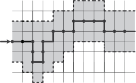
The complexity of the DP algorithm is upper-bounded by the size of the DP table times the complexity of computing each table entry. Denote by the total number of possible coordinates333As a computation / quality tradeoff, we can restrict the set of potential coordinates, for example, to be a set of neighborhood grid points within some fixed distance from the original contour segment ; e.g., the set of points in the grey area in Fig. 5 within from original . . Examining the subscript and three arguments of the recursive function , we see that the DP table size is , or . The complexity of compute one table entry using (24) is . Hence the complexity of the algorithm is .
IV-B3 Total Suffix Tree (TST)
When the training data is large, is also large, resulting in a very large DP table size due to the exponential term . In (24) when calculating local cost , actually the context required to compute rate is , where the context length is typically smaller than because the context tree of maximum depth is variable-length. Thus, if we can, at appropriate recursive calls, reduce the history from of length to of length , , for recursive call to in (24), then we can reduce the DP table size and in turn the computation complexity of the DP algorithm.
The challenge is how to “remember” just enough previous symbols during recursion so that the right context can still be correctly identified to compute rate at a later recursive call. The solution to this problem can be described simply. Let be a context (end node) in context tree . Context must be created at some previous recursive call by concatenating a chosen -th symbol with suffix of context . It implies that the recursion in (24) must remember suffix for this creation of to take place at a later recursion. To create suffix at a later recursive call, one must remember its suffix at an earlier call. We can thus generalize this observation and state that a necessary and sufficient condition to preserve all contexts in context tree is to remember all suffixes of during the recursion.
All suffixes of contexts in can themselves be represented as a tree, which we call a total suffix tree (TST), denoted as . By definition, is a sub-tree of . Further, TST is also a full tree given is a full tree; is essentially a union of all sub-trees of , and a sub-tree of a full tree is also a full tree. has contexts, each of maximum length . Each context can induce additional end nodes in TST . Hence TST has end-nodes.
Fig. 6 illustrates one example of TST derived from the context tree shown in Fig. 3. TST can be used for compact DP table entry indexing during recursion (24) as follows. When an updated history is created from a selection of symbol , we first truncate to , where is the longest matching string in from root node down. Because TST is a full tree, the longest matching string always corresponds to an end node. The shortened history is then used as the new argument for the recursive call. Practically, it means that only DP table entries of arguments that are end nodes of TST will be indexed, thus reducing complexity from original to , which is now polynomial in .
IV-C MADD based Contour Coding
When the distortion metric is MADD, instead of an unconstrained Lagrangian formulation, we formulate instead a distortion-constrained problem as follows:
| (25) |
where is the maximum distortion permitted. Example when is shown in Fig. 5. can be varied to induce different RD tradeoff.
Given the definition of rate and distortion, (25) can be rewritten as:
| (26) |
Similar to the SSDD case, this minimization problem can also be solved by using DP by simplifying the problem to:
| (27) |
where denotes the coding cost of . The problem becomes finding an approximated DCC string in the region restricted by in order to minimize the total rate.
Denote by the minimum total rate from to given the previous symbols , and the previous edge has coordinate and absolute direction . We can compute recursively as follows:
| (28) |
where we restrict to induce only edges that are within the feasible region delimited by . The recursion is same as (24) except the local cost function. Hence the complexity of the DP algorithm here is also same as in the SSDD case.
V Starting Point Coding
(a)
(b)
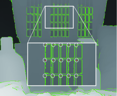
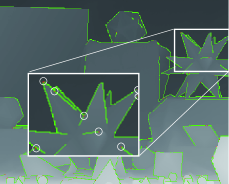
We propose a mixed-Golomb (M-Golomb) algorithm to encode the 2D coordinates of starting points of all contours in the target image. In general, the starting points are not uniformly distributed on the image. They tend to cluster around objects or figures that appear in the scene, as illustrated in Fig. 7. This means that the differences in coordinates of neighboring starting points tend to be small, and Golomb coding [46] is suitable to encode coordinate differences that are more likely small than large.
A 2D coordinate of a starting point has two components (horizontal and vertical); we use Golomb coding to code only the differences in coordinates in one component. Specifically, we first sort the starting points according to this chosen component in ascending order. The coordinate differences in neighboring points are then coded using Golomb coding. The coordinates in the other component are coded using fixed length binary coding.
Golomb coding uses a tunable parameter to divide an input value into two parts: the remainder and the quotient. The quotient is sent in unary coding, followed by the remainder in truncated binary coding. For simplicity, we choose the parameter as , where and is the maximum input value. We examine all possible values of to find the smallest coding cost of all the starting points in the target image and send this selected parameter as side information.
VI Experimental Results
We evaluate the performance of our lossless and lossy contour coding algorithms in three scenarios. For scenario 1, we first present results for lossless contour coding of VOPs in MEPG4 sequences, then results for lossless contour coding of objects in depth images and starting points coding in order. For scenario 2, we present visual comparisons of lossy contour coding of objects in depth images, then show the RD performance of lossy depth image coding. For scenario 3, we present visual comparisons of different silhouette approximating methods, then show the RD performance of lossy multiview silhouette coding for 3D reconstruction.
VI-A Lossless Contour Coding
To evaluate the performance of our proposed context tree based lossless contour coding (CT-LL), we used VOPs of four MPEG4 sequences444ftp://ftp.tnt.uni-hannover.de/pub/MPEG/mpeg4_masks/, Children, Stefan, Robot and Cyc, as test data. The spatial resolution of all four sequences is . 10 frames were tested for each sequence. Note that the contours of the VOPs were already outlined as input to our coding algorithm. We also coded object contours in four Middleburry depth images555http://vision.middlebury.edu/stereo/data/: Moebius (456368), Cones (448368), Teddy (448368) and Laundry (440368). The contours were detected using a gradient-based edge detection scheme in [7].
To code VOPs in a given video frame of a MPEG-4 sequence, previous two frames of the same sequence were used to train the context tree. To code object contours of a Middleburry depth image, we used other Middleburry images to train the context tree. We tested two training image sets (Train1 and Train2), where each contains four different randomly selected images. To test the performance of our proposed CT-LL with different training sets, we used also a combined training image set (Train1+Train2), which contains images in both Train1 and Train2. We set the parameter in all the experiments.
We compared CT-LL against four lossless compression schemes: i) the Lempel-Ziv-Welch (LZW) algorithm in [47], an improved version of LZ78; ii) the probability suffix tree (PST) algorithm in [16], iii) the prediction by partial matching (PPM) algorithm in [48], and iv) the arithmetic edge coding (AEC) scheme in [7]. The training datasets for PST and PPM were the same as those for CT-LL. Our proposed starting points coding scheme (M-Golomb) was compared against fixed length binary coding (Binary). All the contour compression methods used our proposed M-Golomb for coding the starting points in the experiments.
| Bits/Symbol | LZW | AEC | PST | PPM | CT-LL |
|---|---|---|---|---|---|
| Children | 1.685 | 1.256 | 1.176 | 1.257 | 1.170 |
| Stefan | 1.494 | 1.117 | 0.914 | 0.956 | 0.894 |
| Robot | 1.808 | 1.414 | 1.341 | 1.318 | 1.278 |
| Cyc | 1.525 | 1.182 | 0.879 | 0.823 | 0.828 |
| Average | 1.628 | 1.242 | 1.078 | 1.089 | 1.043 |
| Bits/Symbol | LZW | AEC | Train1 | Train2 | Train1+Train2 | ||||||
|---|---|---|---|---|---|---|---|---|---|---|---|
| PST | PPM | CT-LL | PST | PPM | CT-LL | PST | PPM | CT-LL | |||
| Moebius | 1.912 | 1.409 | 1.378 | 1.272 | 1.233 | 1.373 | 1.286 | 1.240 | 1.326 | 1.257 | 1.220 |
| Cones | 1.727 | 1.424 | 1.245 | 1.181 | 1.164 | 1.282 | 1.232 | 1.199 | 1.241 | 1.176 | 1.154 |
| Teddy | 2.014 | 1.519 | 1.555 | 1.493 | 1.450 | 1.550 | 1.493 | 1.434 | 1.510 | 1.479 | 1.439 |
| Laundry | 1.642 | 1.265 | 1.290 | 1.216 | 1.189 | 1.257 | 1.199 | 1.165 | 1.255 | 1.195 | 1.166 |
| Average | 1.824 | 1.404 | 1.367 | 1.291 | 1.259 | 1.366 | 1.303 | 1.260 | 1.333 | 1.277 | 1.245 |
VI-A1 Results for Lossless Contour Coding of VOPs in MPEG4 Sequences
Table II shows the compression results in average bits per symbol for VOP lossless coding using different methods. Compared to the other methods, our proposed CT-LL achieves noticeable bitrate reduction on average. Specifically, on average we reduce the bitrate by 35.97% compared to LZW, 16.08% compared to AEC, 3.26% compared to PST, and 4.23% compared to PPM.
In general, the context based methods (PST, PPM and CT-LL) outperform LZW and AEC significantly. Compared to PPM, the gain of our CT-LL varies depending on different sequences. In particular, for Children and Stefan with large motion, CT-LL outperforms PPM by 6.92% and 6.49%. While for Cyc with very small motion, CT-LL is worse than PPM marginally by 0.60%. Since there is no prior to prune the contexts in PPM, it fails to avoid overfitting for sequences with large motion. Compared to PST, which can avoid overfitting by setting five application-specific thresholds, CT-LL has steady gain because of the our proposed geometric prior for contour coding.
| Input | Average Num | Bits of Starting Points | Total Bits | |||||
| of Contours | Binary | M-Golomb | Bits | Binary | M-Golomb | Bits | ||
| Children | 3.4 | 57.8 | 58.7 | 1.56% | 1684.7 | 1685.6 | 0.05% | |
| Mask | Stefan | 1 | 17 | 21 | 23.53% | 517.1 | 521.1 | 0.77% |
| Seqeunces | Robot | 21.3 | 362.1 | 273.8 | -24.39% | 2474.1 | 2385.8 | -3.57% |
| Cyc | 21.6 | 367.2 | 295.5 | -19.53% | 2959.5 | 2887.8 | -2.42% | |
| Average | 11.8 | 201.0 | 162.3 | -19.29% | 1908.9 | 1870.1 | -2.03% | |
| Moebius | 144 | 2592 | 1785 | -31.13% | 8825 | 8018 | -9.14% | |
| Depth | Cones | 82 | 1476 | 1081 | -26.76% | 7399 | 7004 | -5.34% |
| Images | Teddy | 100 | 1800 | 1289 | -28.39% | 7894 | 7467 | -5.41% |
| Laundry | 125 | 2250 | 1563 | -30.53% | 9254 | 8567 | -7.42% | |
| Average | 112.8 | 2029.5 | 1429.5 | -29.56% | 8343.0 | 7764.0 | -6.94% | |
VI-A2 Results for Lossless Contour Coding of Objects in Middlebury Depth Images
Table III shows the compression results for lossless contour coding of objects in depth images. Our CT-LL outperforms the other four methods for all three training sets. Specifically, for Train1, the average bit reductions are 30.96%, 10.35%, 7.89% and 2.45% over LZW, AEC, PST and PPM, respectively; for Train2, the average bit reductions are 30.93%, 10.30%, 7.76% and 3.31%; for Train1+Train2, the average bit reductions are 31.74%, 11.36%, 6.62% and 2.49%.
Compared to the results of lossless contour coding of VOPs, the performance of CT-LL of lossless contour coding of objects in depth images decreased a bit. The difference mainly stems from the dissimilarity in statistics between the test and training images in the latter case. Specifically, for coding VOPs in MPEG4 video sequences, the training images are the previous frames, which are quite similar to the current frame. While for the test depth images, the training images are randomly selected images, which were obtained using the same setup but from different 3D scenes. Nonetheless, as shown in Table III, we can still achieve bitrate reduction compared to other methods using different training sets.
Comparing the results of Train1+Train2 to that of Train1 and Train2, we can see that all three context based methods (PST, PPM and CT-LL) benefited from more training data, resulting in lower average bitrates. With twice the training data, PST and PPM resulted in a larger improvement compared to CT-LL. This demonstrates that the performance of our proposed CT-LL is stable for large and small data size. In other words, unlike other context based methods like PST and PPM, our CT-LL maintains good coding performance even for small data size by avoiding overfitting using our proposed geometric prior.
VI-A3 Results for Starting Points Coding
The performance of our proposed starting points coding scheme (M-Golomb) compared to the fixed binary coding (Binary) is shown in Table IV. We tested both the VOPs in MPEG4 sequences and the object contours in depth images. Both the number of contours and the bit overhead in coding contours of VOPs are averaged to one frame to better compare to that of the depth images. For the VOPs which contain only a few contours in one frame, i.e., Children and Stefan, the proposed M-Golomb has little advantage over Binary. However, we can save on average 29.56% bits of starting points and 6.94% bits of total bits for the depth images which contain lots of contours in one image.
VI-B Depth Image Coding
We implemented our proposed SSDD based lossy contour coding (CT-SSDD) scheme for coding edges as side information in MR-GFT [4], one of the state-of-the-art depth image compression methods. In [4], the detected edges of the whole image are losslessly coded by employing AEC [7] and transmitted to the decoder for directional intra prediction. We replace AEC with CT-SSDD to compress four Middleburry depth images which are same as that in section VI-A. Train2 are used as the training images.
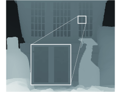
Different from the losslessly edge coding in MR-GFT, we compressed contours lossily using our proposed CT-SSDD. Changes in the contours can lower the edge coding cost, but can also lead to larger intra prediction residual. We thus augmented the depth image to match the approximated edges obtained using CT-SSDD, in order to reduce the prediction residual. Specifically, the pixel values between the original edge and the approximated edge were replaced with the pixel values on the other side of the approximated edge, as shown on Fig. 8.
Since the contours are coded as side information for compressing depth images, the distortion term in CT-SSDD should be related to the distortion of the depth signal. Distortion of our described depth image coding scheme comes from two sources: i) distortion due to quantization of the transform coefficients, and ii) distortion due to depth pixel augmentation to suit approximated contours, as described previously. Because the contour coding and the residual coding in MR-GFT are performed in separate steps, it is impractical to consider both distortions simultaneously.
As a straightforward attempt, the distortion term in (17) is modified and defined as the augmentation distortion, which is calculated as the sum of squared distortion of augmented depth pixels instead of the approximated symbols. Further, we choose , which is the same as used in the mode selection part of MR-GFT, where is the quantization parameter. Thus this selection of provides an appropriate weight between the edge coding and the residual coding.
We compare the depth image coding performance of our proposed MR-GFT+CT-SSDD against MR-GFT+CT-LL, MR-GFT+PPM, the original MR-GFT in [4] and HEVC Test Model HM-16.0666https://hevc.hhi.fraunhofer.de/svn/svn_HEVCSoftware/tags/HM-16.0/ (HEVC), where MR-GFT+CT-LL and MR-GFT+PPM are obtained by replacing the edge coding scheme (AEC) in MR-GFT with the proposed CT-LL and PPM.

(a)
(b)

(c)
(d)
VI-B1 Edge Approximation and Depth Image Augmentation
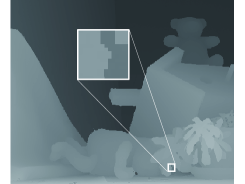
Fig. 8 shows two examples of edge approximation and depth image augmentation. We see that the changed edges are mostly the irregular edges (e.g., the white region in Fig. 8). This is because these irregular edges along with their contexts have more scattered probability distributions in the trained context tree , which will consume larger amount of bits after arithmetic coding. As shown in Fig. 8, after approximating the edges, the depth pixels are augmented to match the new edges.
Note that edges with smaller gradient (e.g., mesh grid of basket in Fig. 8(b) and flower in Fig. 8(d)) are more likely to be approximated than edges with larger gradient (e.g., the boundaries of basket in Fig. 8(b) and Teddy bear in Fig. 8(d)). This is because approximation of the edges with larger gradient will result in larger augmentation distortion.
| QP | MR-GFT | MR-GFT | MR-GFT | ||||||
|---|---|---|---|---|---|---|---|---|---|
| CT-LL | CT-SSDD | ||||||||
| Edge | Resi | Total | Edge | Resi | Total | Edge | Resi | Total | |
| 22 | 6515 | 12132 | 18647 | 6178 | 12132 | 18310 | 6160 | 12132 | 18292 |
| 27 | 6515 | 7857 | 14372 | 6178 | 7857 | 14035 | 6101 | 7854 | 13955 |
| 32 | 6515 | 6225 | 12740 | 6178 | 6225 | 12403 | 5827 | 6021 | 11848 |
| 37 | 6515 | 5344 | 11859 | 6178 | 5344 | 11522 | 5548 | 5322 | 10870 |
(a)
(b)
(c)
(d)
VI-B2 Results in RD Performance
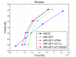
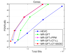
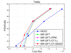
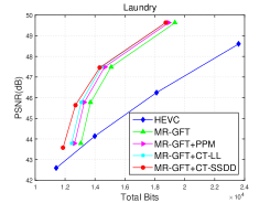
The RD performance of the proposed MR-GFT+CT-SSDD and MR-GFT+CT-LL against MR-GFT+PPM, MR-GFT and HEVC is presented in Fig. 9. The proposed MR-GFT+CT-SSDD achieves promising bit rate reduction over a wide range of PSNR, and the proposed MR-GFT+CT-LL also outperforms other three schemes. On average, we achieve a bit rate reduction of 19.34% over HEVC, 10.29% over MG-GFT, 5.02% over MR-GFT+PPM and 3.46% over MR-GFT+CT-LL.
Compared to MR-GFT, the gain of the proposed two schemes comes from the more efficient edge coding schemes. Table V gives the detailed results of bits of coding edges among the total bits with different of Teddy. When , we save on average 14.84% bits and 5.17% bits for coding edges with the proposed CT-SSDD and CT-LL compared to AEC adopted in MR-GFT. Note that the bits of coding residuals (difference between total bits and bits of coding edges) of MR-GFT+CT-LL and MR-GFT are the same, while they are a bit larger than that of MR-GFT+CT-SSDD. Using MR-GFT+CT-SSDD, the depth image is augmented with fewer irregular edges before coding, resulting in more efficient directional intra prediction.
The bit rate reduction of CT-SSDD over CT-LL becomes larger when the increases. This is also reflected in the RD curve in Fig. 9. As previously discussed, the strength of the approximation is controlled by . When is small, is also small which makes the edges less likely be changed. In other words, in high bit rate situation, it is unnecessary to approximate the edges, while more edges can be changed in the low bit rate situation.

(a)
(b)
(c)
VI-C Multiview Silhouettes Coding for 3D Reconstruction
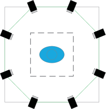
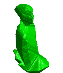
We test our proposed MADD based lossy contour coding CT-MADD on the multiview silhouette sequences from Microsoft Research. The sequences are obtained using the equipment set up in [49]. The spatial resolution of the silhouettes is . Each sequence contains 10 frames, and eight views are taken for each frame. Fig. 10(a) shows an example of the silhouettes of eight views for a single frame. The silhouettes were extracted from the images captured with an eight camera rig, as illustrated in Fig. 10(b). With the extracted silhouettes, the 3D model can be reconstructed as shown in Fig. 10(c). We coded four multiview silhouette sequences using CT-MADD and reconstructed the 3D models with the coded silhouettes. The RD performance was evaluated, where distortion is the volume error between the 3D model reconstructed with the original silhouettes and that with the coded silhouettes.
The 3D model was reconstructed based on a volume intersection scheme [50]. We projected each silhouette onto an initialized 3D volume and the final 3D model is the intersected volume of the eight projected silhouettes.
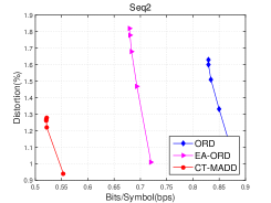
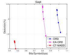
We compare the RD performance of CT-MADD against two lossy contour compression schemes: the operational rate-distortion optimal polygon-based shape coding (ORD) in [9] and the improved version based on an adaptive edge coding scheme (EA-ORD) in [12]. ORD and EA-ORD also adopt the MADD measure same as the proposed CT-MADD. For all three methods, was set from 1 to 5 to test different distortion.

(a) 1429 bits

(b) 1179 bits

(c) 664 bits

(d) 1376 bits

(e) 1128 bits

(f) 646 bits
VI-C1 Comparison of Contour Approximation
Fig. 11 shows one view of silhouette approximation using different methods with and . With the same , CT-MADD consumes the fewest bits to code the silhouette. As for subjective quality, the silhouettes approximated by CT-MADD are most similar visually to the original silhouettes, while the results by ORD and EA-ORD contain lots of staircase shapes.
In both ORD and EA-ORD, only some contour pixels are selected for coding. The approximated silhouette was constructed by connecting these selected contour pixels in order, making the result unnatural with too many staircase lines.
(a)
(b)

(c)
(d)
VI-C2 Evaluation of RD Performance
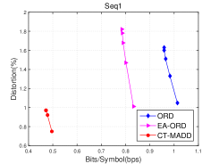
The RD performance is shown in Fig. 12. We observe that CT-MADD outperforms ORD and EA-ORD significantly both in bit rate and distortion. Specifically, at the same , CT-MADD has an average bitrate reduction of 50% and 38% and an average of distortion reduction of 31% and 43% compared to ORD and EA-ORD.
In ORD and EA-ORD, the differences between two selected contour pixels (vertices) are coded using unary code. Larger differences will consume more bits. Although CT-MADD codes more number of contour pixels, the accurately estimated conditional probabilities enable our contour pixels to be coded much more efficiently than ORD and EA-ORD.
VII Conclusion
We investigate the problem of lossless and lossy coding of image contours, focusing on the case when the sizes of training datasets are limited. To avoid overfitting, we propose a maximum a posteriori (MAP) formulation to compute an optimal variable-length context tree (VCT) —one that has both large likelihood that can explain observed data , and large prior stating that contours are more likely straight than curvy. For the lossy case, we develop dynamic programming (DP) algorithms that approximate a detected contour by trading off coding rate with two different notions of distortion. The complexity of the DP algorithms can be reduced via compact table entry indexing using a total suffix tree (TST) derived from VCT . Experimental results show that our proposed lossless and lossy algorithms outperform state-of-the-art coding schemes consistently for both small and large training datasets.
References
- [1] C. Grigorescu, N. Petkov and M. A. Westenberg, “Contour detection based on nonclassical receptive field inhibition,” IEEE Trans. Image Process., vol. 12, no. 7, pp. 729–739, 2003.
- [2] G. Shen, W.-S. Kim, S.K. Narang, A. Ortega, J. Lee, and H. Wey, “Edge-adaptive transforms for efficient depth map coding,” in IEEE Picture Coding Symposium, Nagoya, Japan, December 2010.
- [3] W. Hu, G. Cheung, X. Li, and O. Au, “Depth map compression using multi-resolution graph-based transform for depth-image-based rendering,” in IEEE International Conference on Image Processing, Orlando, FL, September 2012.
- [4] W. Hu, G. Cheung, A. Ortega, and O. Au, “Multi-resolution graph Fourier transform for compression of piecewise smooth images,” in IEEE Transactions on Image Processing, January 2015, vol. 24, no.1, pp. 419–433.
- [5] W. Hu, G. Cheung, and A. Ortega, “Intra-prediction and generalized graph Fourier transform for image coding,” in IEEE Signal Processing Letters, November 2015, vol. 22, no.11, pp. 1913–1917.
- [6] I. Daribo, D. Florencio, and G. Cheung, “Arbitrarily shaped sub-block motion prediction in texture map compression using depth information,” in 2012 Picture Coding Symposium, Krakow, Poland, May 2012.
- [7] I. Daribo, D. Florencio and G. Cheung, “Arbitrarily shaped motion prediction for depth video compression using arithmetic edge coding,” IEEE Trans. Image Process., vol. 23, no. 11, pp. 4696–4708, Nov. 2014.
- [8] D. Weinland, R. Ronfard and E. Boyer, “A survey of vision-based methods for action representation, segmentation and recognition,” Computer Vision and Image Understanding, vol. 115, no. 2, pp. 224–241, 2011.
- [9] A. K. Katsaggelos, L. P. Kondi, F. W. Meier, W. Fabian, J. O. Ostermann and G. M. Schuster, “MPEG-4 and rate-distortion-based shape-coding techniques,” Proceedings of the IEEE, vol. 86, no. 6, pp. 1126–1154, 1998.
- [10] F. Sohel, G. C. Karmakar, L. S. Dooley and M. Bennamoun, “Sliding-window designs for vertex-based shape coding,” IEEE Trans. Multimedia, vol. 14, no. 3, pp. 683–692, 2012.
- [11] Z. Lai, J. Zhu, Z. Ren, W. Liu, and B. Yan, “Arbitrary directional edge encoding schemes for the operational rate-distortion optimal shape coding framework,” in Proc. Conf. Data Compression. IEEE, 2010, pp. 20–29.
- [12] J. H. Zhu, Z. Y. Lai, W. Y. Liu and J. B. Luo, “Adaptive edge encoding schemes for the rate-distortion optimal polygon-based shape coding,” in Proc. Conf. Data Compression, 2014, pp. 103–112.
- [13] R. El-Yaniv R. Begleiter and G. Yona, “On prediction using variable order markov models,” Journal of Artificial Intelligence Research, pp. 385–421, 2004.
- [14] J. Rissanen, “A universal data compression system,” IEEE Trans. Information Theory, vol. 29, no. 5, pp. 656–664, 1983.
- [15] J. Cleary and I. Witten, “Data compression using adaptive coding and partial string matching,” IEEE Trans. Commun., vol. 32, no. 4, pp. 396–402, 1984.
- [16] D. Ron, Y. Singer and N. Tishby, “The power of amnesia: Learning probabilistic automata with variable memory length,” Machine learning, vol. 25, no. 2-3, pp. 117–149, 1996.
- [17] C. C. Lu and J. G. Dunham, “Highly efficient coding schemes for contour lines based on chain code representations,” IEEE Trans. Commun., vol. 39, no. 10, pp. 1511–1514, 1991.
- [18] M. Armbrust, A. Fox, R. Griffith, A. D. Joseph, Anthony D and R. Katz, “A view of cloud computing,” Communications of the ACM, vol. 53, no. 4, pp. 50–58, 2010.
- [19] R. W. Katz, “On some criteria for estimating the order of a markov chain,” Technometrics, vol. 23, no. 3, pp. 243–249, 1981.
- [20] P. Vandewalle, J. Kovačević and M. Vetterli, “Reproducible research in signal processing,” IEEE Signal Processing Mag., vol. 26, no. 3, pp. 37–47, 2009.
- [21] H. Freeman, “Application of the generalized chain coding scheme to map data processing,” 1978, pp. 220–226.
- [22] Y. Liu and B. Žalik, “An efficient chain code with huffman coding,” Pattern Recognition, vol. 38, no. 4, pp. 553–557, 2005.
- [23] Y. H. Chan and W. C. Siu, “Highly efficient coding schemes for contour line drawings,” in Proc. IEEE Int. Conf. Image Process. IEEE, 1995, pp. 424–427.
- [24] R. Estes and R. Algazi, “Efficient error free chain coding of binary documents,” in Proc. Conf. Data Compression, 1995, p. 122.
- [25] M. J. Turner and N. E. Wiseman, “Efficient lossless image contour coding,” in Computer Graphics Forum, 1996, vol. 15, no.2, pp. 107–117.
- [26] O. Egger, F. Bossen and T. Ebrahimi, “Region based coding scheme with scalability features,” in Proc. Conf. VIII European Signal Processing. IEEE, 1996, vol. 2, LTS-CONF-1996-062, pp. 747–750.
- [27] C. Jordan, S. Bhattacharjee, F. Bossen, F. Jordan, and T. Ebrahimi, “Shape representation and coding of visual objets in multimedia applications—an overview,” Annals of Telecommunications, vol. 53, no. 5, pp. 164–178, 1998.
- [28] H. Freeman, “On the encoding of arbitrary geometric configurations,” IRE Trans. Electronic Computers, , no. 2, pp. 260–268, Jun 1961.
- [29] I. Daribo, G. Cheung and D. Florencio, “Arithmetic edge coding for arbitrarily shaped sub-block motion prediction in depth video coding,” in IEEE International Conference on Image Processing, Orlando, FL, September 2012.
- [30] T. Kaneko and M. Okudaira, “Encoding of arbitrary curves based on the chain code representation,” IEEE Trans. Commun., vol. 33, no. 7, pp. 697–707, 1985.
- [31] J. Ziv and A. Lempel, “A universal algorithm for sequential data compression,” IEEE Trans. Information Theory, vol. 23, no. 3, pp. 337–343, 1977.
- [32] P. Bühlmann and A. J. Wyner, “Variable length markov chains,” The Annals of Statistics, vol. 27, no. 2, pp. 480–513, 1999.
- [33] G. Bejerano and G. Yona, “Variations on probabilistic suffix trees: statistical modeling and prediction of protein families,” Bioinformatics, vol. 17, no. 1, pp. 23–43, 2001.
- [34] M. C. Yeh, Y. L. Huang and J. S. Wang, “Scalable ideal-segmented chain coding,” in Proc. IEEE Int. Conf. Image Process., 2002, vol. 1, pp. 194–197.
- [35] S. Zahir, K. Dhou and B. Prince George, “A new chain coding based method for binary image compression and reconstruction,” 2007, pp. 1321–1324.
- [36] J. Chung, J. Lee, J. Moon and J. Kim, “A new vertex-based binary shape coder for high coding efficiency,” Signal processing: image communication, vol. 15, no. 7, pp. 665–684, 2000.
- [37] C. Kuo, C. Hsieh and Y. Huang, “A new adaptive vertex-based binary shape coding technique,” Image and vision computing, vol. 25, no. 6, pp. 863–872, 2007.
- [38] G. M. Schuster and A. K. Katsaggelos, “An optimal segmentation encoding scheme in the rate distortion sense,” in Proc. IEEE Int. Symp. Circuits and Systems, May 1996, vol. 2, pp. 640–643.
- [39] G. M. Schuster, G. Melnikov and A. K. Katsaggelos, “Operationally optimal vertex-based shape coding,” IEEE Signal Processing Mag., vol. 15, no. 6, pp. 91–108, 1998.
- [40] F. A. Sohel, L. S. Dooley and G. C. Karmakar, “Variable width admissible control point band for vertex based operational-rate-distortion optimal shape coding algorithms,” in Proc. IEEE Int. Conf. Image Process. IEEE, 2006, pp. 2461–2464.
- [41] F. A. Sohel, L. S. Dooley and G. C. Karmakar, “New dynamic enhancements to the vertex-based rate-distortion optimal shape coding framework,” IEEE Trans. Circuits Syst. Video Technol., vol. 17, no. 10, pp. 1408–1413, 2007.
- [42] S. Alcaraz-Corona and R. Rodríguez-Dagnino, “Bi-level image compression estimating the markov order of dependencies,” IEEE Journal of Selected Topics in Signal Processing, vol. 4, no. 3, pp. 605–611, 2010.
- [43] A. Akimov, A. Kolesnikov and P. Fränti, “Lossless compression of map contours by context tree modeling of chain codes,” Pattern Recognition, vol. 40, no. 3, pp. 944–952, 2007.
- [44] S. Kullback, “Letter to the editor: the kullback-leibler distance,” 1987.
- [45] D. Neuhoff and K. G. Castor, “A rate and distortion analysis of chain codes for line drawings,” IEEE Trans. Information Theory, vol. 31, no. 1, pp. 53–68, 1985.
- [46] S. W. Golomb, “Run-length encodings,” IEEE Trans. Information Theory, 1966.
- [47] T. A. Welch, “A technique for high-performance data compression,” Computer, vol. 6, no. 17, pp. 8–19, 1984.
- [48] A. Moffat, “Implementing the ppm data compression scheme,” IEEE Trans. Communications, vol. 38, no. 11, pp. 1917–1921, 1990.
- [49] C. Loop, C. Zhang and Z. Y. Zhang, “Real-time high-resolution sparse voxelization with application to image-based modeling,” in Proc. ACM Conf. High-Performance Graphics, 2013, pp. 73–79.
- [50] W. N. Martin and J. K. Aggarwal, “Volumetric descriptions of objects from multiple views,” IEEE Trans. Pattern Analysis and Machine Intelligence, , no. 2, pp. 150–158, 1983.