Gravitational waveforms from binary neutron star mergers
with high-order WENO schemes in numerical relativity

Abstract

The theoretical modeling of gravitational waveforms from binary neutron star mergers requires precise numerical relativity simulations. Assessing convergence of the numerical data and building the error budget is currently challenging due to the low accuracy of general-relativistic hydrodynamics schemes and to the grid resolutions that can be employed in $(3+1)$-dimensional simulations. In this work, we explore the use of high-order weighted-essentially-nonoscillatory (WENO) schemes in neutron star merger simulations and investigate the accuracy of the waveforms obtained with such methods. We find that high-order WENO schemes can be robustly employed for simulating the inspiral-merger phase and they significantly improve the assessment of the waveform’s error budget with respect to finite-volume methods. High-order WENO schemes can be thus efficiently used for high-quality waveforms production, also in future large-scale investigations of the binary parameter space.

I Introduction

Gravitational-wave (GW) astronomy has started with the first direct observation of a merging binary black hole system Abbott et al. (2016). Beside black hole binaries, binary neutron stars (BNS) are one of the main expected sources for the advanced GW detectors Aasi et al. (2013). The BNS parameters estimation, including the NS’s equation of state, in near-future detection requires models of merger waveforms. An example of such a model is the tidal effective-one-body model we have recently developed in Bernuzzi et al. (2015), which is compatible with numerical relativity (NR) data up to merger (peak of the waveform’s amplitude) Bernuzzi et al. (2015). Developing and improving the accuracy of these analytical models crucially relies on the availability of precise NR waveforms. This paper reports on our latest effort towards the production of NR waveforms from BNSs.

Key issues for producing high-quality NR waveforms are (1) the assessment of the convergence properties of the numerical data at increasing grid resolutions and (2) the production of a trustworthy error budget. Different NR groups have considered this problem Baiotti et al. (2009); Bernuzzi et al. (2012a, b); Reisswig et al. (2013); Radice et al. (2014a); Hotokezaka et al. (2013); Bernuzzi et al. (2015); Hotokezaka et al. (2015); Haas et al. (2016) and showed that 3+1 NR simulations including general-relativistic hydrodynamics (GRHD) can deliver waveforms with phase uncertainties of $\delta\phi\lesssim 3$ rad Radice et al. (2014a); Bernuzzi et al. (2015); Hotokezaka et al. (2015) accumulated over the last $\sim 10-20$ orbits to merger . These are rather accurate results but, on the one hand, convergence and error bars are typically difficult to estimate (see below), and, on the other hand, the improvements of the current analytical models require computations at higher precision Bernuzzi et al. (2015).

All previous works agree on that the truncation error of the GRHD solver is the main source of uncertainty in BNS simulations, e.g. Bernuzzi et al. (2012a); Hotokezaka et al. (2013); Radice et al. (2014a). The numerical dissipation of the second-order-accurate shock-capturing algorithms employed for the solution of GRHD, combined with the typical 3D grid resolutions, can dramatically affect the accuracy of the phase evolution of the binary Bernuzzi et al. (2012b). The use of nonlinear limiters in shock-capturing schemes introduces systematic errors that are difficult to quantify Bernuzzi et al. (2012b). Furthermore, measuring the convergence rate of the numerical solution is challenging because of the limited span in grid resolutions that can be achieved in 3D simulations Bernuzzi et al. (2012a). And in absence of a clear convergence measure, the evaluation of truncation errors is impossible. Improving the numerical schemes for GRHD is thus necessary for future development of the field.

In a series of seminal work in the 1990s Harten et al. (1987); Harten (1989); Shu and Osher (1989a, b); Liu et al. (1994); Jiang (1996), Harten, Shu and others developed high-order finite-differencing flux-conservative schemes for hydrodynamics. These schemes rely on three elements: projection of the fluxes on characteristic fields, the flux-splitting approach, and high-order–essentially-nonoscillatory interpolation procedures (reconstruction). A particularly efficient reconstruction is the fifth-order weighted-essentially-nonoscillatory (WENO) interpolation scheme of Jiang (1996), which is very well known in the computational physics literature. Such WENO high-order algorithms are natural candidates for NR codes and BNS evolutions for several reasons: (i) they can achieve high-order accuracy for sufficiently smooth solution; (ii) they are developed for uniform grids and Runge-Kutta (RK) time stepping, which are both standard techniques in NR; (iii) they are consistent with the finite-differencing treatment used for the metric fields; (iv) and they can be easily implemented in multidimensions.

Radice et al. presented, for the first time in the context of NR, BNS merger simulations employing a high-order finite-differencing algorithm Radice et al. (2014a, b, 2015, 2016). The latter is very similar to the WENO method mentioned above, the only difference being the use of the fifth-order monotonicity preserving (MP5) scheme of Suresh et al. Suresh (1997). BNS simulations benefit from the use of the high-order scheme. In particular, third-order convergence was observed for the waveform’s phase using four simulations at different resolutions Radice et al. (2015, 2016). The MP5-based high-order scheme has been also recently used for the simulations presented in Hinderer et al. (2016), although no detailed convergence analysis has been presented there.

In this work we assess, for the first time, the use of high-order WENO schemes for the computation of GWs from BNS inspiral-merger simulations. We focus on the accuracy of the GW phase error and show that, although the scheme does not achieve the formal high-order accuracy, convergence can be clearly monitored at typical 3D grid resolutions. The error budget is then robustly determined by combining numerical data from different grid resolutions and using Richardson extrapolation. We also consider the MP5 scheme Suresh (1997) for comparison with previous work, but we do not find this method as robust as the WENO one in our simulations.

The paper is organized as follows. Sec. II summarizes the relevant equations. Sec. III describes the numerical methods; and it is complemented by Appendix A in which our implementation is validated against standard test problems. Sec. IV describes numerical evolutions of single star spacetimes with the high-order scheme. Sec. V describes numerical evolutions of inspiral-merger BNS with the high-order WENO scheme. Focus is on convergence of the data for increasing grid resolutions. Sec. VII discusses error estimates for our BNS waveforms. Throughout this work we use geometric units setting $c=G=1$ and masses are expressed in $M_{\odot}$.

II GRHD and Dynamical Spacetimes

In this section we briefly review the equations governing relativistic flows on dynamical spacetimes in 3+1 NR, as used in this work. The problem is defined by a PDE system composed of GRHD in conservation form Font (2007),

$$\partial_{t}\mathbf{q}=-\partial_{i}\mathbf{f}^{(i)}+\mathbf{s}\ ,$$ (1)

coupled to a 3+1 hyperbolic formulation of the metric equations, schematically

$$\partial_{t}\mathbf{u}={\cal{N}}\left(\partial^{2}_{i}\mathbf{u},\partial_{i}\mathbf{u},\mathbf{u};\mathbf{w}\right)\ .$$ (2)

In Eq. (1), $\mathbf{q}$ is a state vector collecting the conserved variables, $\mathbf{f}$ are the hydrodynamical fluxes, and $\mathbf{s}$ is a source term depending on metric fields and primitive variables. The conserved variables are $\mathbf{q}=\sqrt{\gamma}(D,\,S_{k},\,\tau)$, and represent the rest mass density ($D$), the momentum density ($S_{k}$), and an internal energy ($\tau$) of the Eulerian observers that define the spacetime foliation. The quantity $\gamma=\det\gamma_{ij}$ is the determinant of the spatial metric in the 3+1 decomposition of Einstein equations. Conserved variables can be written in terms of the primitive variables $\mathbf{w}=(\rho,v^{i},\epsilon,p)$, i.e. rest mass density, 3-velocity, internal energy, and pressure of the fluid (comoving frame). An equation of state (EOS) closes the system by specifying the pressure in terms of the density $\rho$ and internal energy $\epsilon$. In this work, the neutron star matter is described by either a $\Gamma$-law EOS, $p=(\Gamma-1)\rho\epsilon$, or a more realistic, zero temperature, SLy and MS1b EOS Douchin and Haensel (2001). Isentropic evolutions of $\Gamma$-law EOS models are sometimes imposed by specifying a polytropic EOS, $p=K\rho^{\Gamma}$, $K=const$ and without evolving the GRHD equation for $\tau$, which is then redundant. The zero temperature EOS are implemented by a piecewise polytrope fit Read et al. (2009), and thermal effects are modeled by an additive pressure contribution given by the $\Gamma$-law EOS with $\Gamma=1.75$ Shibata et al. (2005); Bauswein et al. (2010); Thierfelder et al. (2011a).

Let us briefly comment on the metric equations. In Eq. (2), $\mathbf{u}$ is a state vector collecting the components of the tensorial metric variables, and the right-hand-side (r.h.s) operator ${\cal N}$ is a nonlinear function quadratic in the field variables and first derivatives. As common in 3+1 numerical relativity, we employ a free evolution approach to Einstein equations. During the evolution of constraint satisfying (consistent) initial data, Einstein equations can be violated at the numerical error level. The choice of an appropriate formulation of general relativity is a key point for controlling and reducing these violations. In this work, we use the Z4c formulation proposed in Bernuzzi and Hilditch (2010) (see also Hilditch et al. (2013)) and the BSSNOK system Nakamura et al. (1987); Shibata and Nakamura (1995); Baumgarte and Shapiro (1999). The system in Eq. (2) contains evolution equations for the gauge, i.e. the lapse and shift evolution equations. We use the moving puncture gauge implemented as described in Brügmann et al. (2008); Thierfelder et al. (2011b); Hilditch et al. (2013).

III Numerical Framework

III.1 Grid tructure and evolution algorithm

Our simulations are performed with the BAM code Dietrich et al. (2015); Thierfelder et al. (2011a); Brügmann et al. (2008). The equations described above are numerically solved by explicit time evolution of the initial data. The evolution algorithm is based on the method of lines with explicit RK time integrators. A portion of the spacelike hypersurfaces $\Sigma_{t}$ is covered by logically Cartesian overlapping grids. The strong-field region is covered by a hierarchy of cell-centered and nested Cartesian grids. The hierarchy consists of $L$ levels of refinement labeled by $l=0,...,L-1$. A refinement level consists of one or more Cartesian boxes with constant grid spacing $h_{l}$ on level $l$. A refinement factor of 2 is used such that $h_{l}=h_{0}/2^{l}$. The grids are properly nested in that the coordinate extent of any grid at level $l$, $l>0$, is completely covered by the grids at level $l-1$. Some of the mesh refinement levels $l>l^{mv}$ can be dynamically moved and adapted during the time evolution. We use $n$ points per direction per fixed level, and $n^{mv}$ points per direction per moving level. For some cases, we cover the wave zone $l=L-1$ by a cube-sphere multipatch grid with $n_{r}$ point in the radial direction and $n_{\theta,\phi}\sim n/2$ in the angular ones.

The grid is evolved in time using the Berger-Oliger algorithm Berger and Oliger (1984). We employ fourth- and third-order RK with a Courant-Friedrich-Lewy (CFL) factor of $0.25$ in all the neutron star tests. (For some simulations we tested a lower CFL condition, but see no significant change in the convergence behavior.) Six buffer zones per side per direction are employed for the Berger-Oliger algorithm interpolations. The restriction and prolongation is performed with a fourth-order WENO scheme for the matter fields, and a sixth-order Lagrangian scheme for the metric fields. Contrary to our latest simulations, no additional correction step is employed here for the conservative variables Dietrich et al. (2015). The chosen grid setup already guarantees excellent mass conservation during the inspiral-merger.

The metric field derivatives in (2) are approximated by fourth-order accurate finite-differencing stencils. Sixth-order artificial dissipation operators are employed to stabilize noise from mesh refinement boundaries. The high-order scheme implemented for GRHD is described below. In our previous work, GRHD equations were solved with a second-order scheme composed of the local Lax-Friedrich (LLF) scheme for the fluxes, and primitive reconstruction. We found that the WENOZ reconstruction, among several tested, is particularly accurate for neutron star evolutions Bernuzzi et al. (2012b). Hence, it is chosen here for comparison with the high-order scheme.

In order to simulate vacuum regions, a static, low-density, and cold atmosphere is added in the vacuum region outside the star Thierfelder et al. (2011a). The atmosphere density is chosen as

$$\rho_{atm}=f_{atm}\max\rho(t=0)\ ,$$ (3)

and grid points below a threshold $\rho_{thr}=f_{thr}\rho_{atm}$ are set to $\rho_{atm}$. As we see, the low-density flow is one of the main sources of error in the neutron star simulations (see also e.g. Radice et al. (2014b) for discussions). In this work, we did not attempt to modify our standard atmosphere prescription because we aimed at comparing the higher-order flux scheme with our current “best” second-order scheme. Note that all the numerical relativity implementations make use of similar assumptions and algorithms at low densities as those employed here. In general, it is challenging to deal with matter/vacuum interfaces in the presence of gravitational fields, even without the complication of dynamical spacetimes. See, however, Xing and Shu (2012) for an attempt in the case of a static and Newtonian gravitational field.

III.2 High-order finite-differencing schemes

In this section we briefly review the high-order (HO) finite-differencing scheme Shu and Osher (1989b); Liu et al. (1994); Jiang (1996); Mignone et al. (2010). The presentation is restricted to 1D without loss of generality: a multidimensional scheme is simply obtained by considering fluxes in each direction separately and adding them in the r.h.s.. We assume a 1D uniform mesh $x_{i}$ with $i=1,...,n$ and spacing $h$. Cell interfaces are indicated with $x_{i+1/2}=x_{i}+h/2$ and the pointwise values of a function $f_{i}=f(x_{i})$. Following Shu and Osher (1989b) the divergence term in (1) is calculated using the conservative finite-differencing formula

$$\frac{\partial f}{\partial x}(x_{i})=h^{-1}\left(\hat{F}_{i+1/2}-\hat{F}_{i-1/2}\right)\ ,$$ (4)

where the numerical fluxes at the interfaces, $\hat{F}_{i+1/2}$, are a high-order nonoscillatory approximation of the so-called numerical flux function. The approximation is computed using pointwise values $f_{i}$, identifying them as the cell-averages of another function, and applying reconstruction via primitive function Shu and Osher (1989b).

The numerical fluxes for the GRHD system are built using a flux-splitting approach based on the LLF and performing the reconstruction on the characteristic fields Jiang (1996); Suresh (1997); Mignone et al. (2010). Specifically, the characteristic fields are given by projections of the positive and negative part of the flux onto the left eigenvectors matrix of the Jacobian $\partial\mathbf{f}/\partial\mathbf{q}$ computed at ${i+1/2}$. The $k$th characteristic fields read (cf. Eq. (17) of Mignone et al. (2010))

$$\hat{F}^{(k)\pm}_{({i+1/2}),S}=\frac{1}{2}\mathbf{L}^{(k)}_{i+1/2}\cdot\left(\mathbf{f}_{S}\pm a^{(k)}\mathbf{q}_{S}\right)\ ,$$ (5)

where $\mathbf{L}^{(k)}_{i+1/2}$ is the $k$th left eigenvector matrix computed at ${i+1/2}$, ^± indicate the positive and negative flux, $S$ is an appropriate stencil to be used in the reconstruction (see below), and

$$a^{(k)}=\max_{S}(|\lambda^{(k)}|)$$ (6)

are the maximum of the absolute values $k$th characteristic speeds on $S$. The intercell characteristic fields are obtained applying a reconstruction algorithm,

$$\hat{F}^{(k)\pm}_{i+1/2}=\mbox{Rec}\left[\hat{F}^{(k)\pm}_{(i+1/2),S}\right]\ ,$$ (7)

here indicated by the operator $\mbox{Rec}[.]$. The latter uses the characteristic fields on the stencil $S$ [e.g. Eq.(4.2) of Jiang (1996)]. The numerical fluxes are finally obtained projecting back the characteristic fields

$$\hat{\mathbf{F}}_{i+1/2}=\sum_{k}\left(\hat{F}^{(k)+}_{i+1/2}+\hat{F}^{(k)-}_{i+1/2}\right)\mathbf{R}^{(k)}_{i+1/2}\ .$$ (8)

The left (right) $\mathbf{L}^{(k)}_{i+1/2}$ ($\mathbf{R}^{(k)}_{i+1/2}$) eigenvectors at ${i+1/2}$ are computed from arithmetic averages of $i$ and $i+1$ values. Their expression for GRHD can be found in Font (2007). We compute averages of primitives (except pressure) and metric functions only, and compute the other quantities from these averages. Note that other, nonequivalent procedures for computing the averaged eigenvectors are possible. We have checked some of them and found no differences in the tests of Appendix A.

The HO scheme above is completed by specifying a reconstruction procedure. Here, we consider the fifth-order WENOZ Borges et al. (2008) and MP5 Suresh (1997) algorithms following the implementation of Mignone et al. (2010). A fifth-order WENO uses five points stencil $S^{+}=(i-2,...,i+2)$ to reconstruct the grid function $f_{i}$ at the interface ,

$$f_{{i+1/2}}=\mbox{Rec}\left[f_{S^{+}}\right]=\frac{\omega_{0}}{6}\left(2f_{i-2}-7f_{i-1}+11f_{i}\right)$$ (9)

$$+\frac{\omega_{1}}{6}\left(-f_{i-1}+5f_{i}+2f_{i+1}\right)+\frac{\omega_{2}}{6}\left(2f_{i}+5f_{i+1}-f_{i+2}\right)\ .$$

The weights are nonlinear functions $\omega_{j}=\alpha_{j}/\sum_{j=0}^{2}\alpha_{j}$ of smoothness indicators $\beta_{j}$, and they sum up to unity $\sum_{j}\omega_{j}=1$. For WENOZ one has Borges et al. (2008)

$$\alpha_{j}=o_{j}\left(1+\frac{|\beta_{0}-\beta_{2}|}{\beta_{j}+\varepsilon}\right)\ ,$$ (10)

with $\varepsilon=10^{-42}$, optimal weights $o_{j}=(1/10,6/10,3/10)$ corresponding to the Lagrangian five points interpolation, and

$$\beta_{0} =\frac{13}{12}(f_{i-2}-2f_{i-1}+f_{i})^{2}+\frac{1}{4}(f_{i-2}-4f_{i-1}+3f_{i})^{2}$$ (11a)

$$\beta_{1} =\frac{13}{12}(f_{i-1}-2f_{i}+f_{i+1})^{2}+\frac{1}{4}(f_{i-1}-f_{i+1})^{2}$$ (11b)

$$\beta_{2} =\frac{13}{12}(f_{i}-2f_{i+1}+f_{i+2})^{2}+\frac{1}{4}(3f_{i}-4f_{i+1}+f_{i+2})^{2}$$ (11c)

Smoothness indicators are derived from cell-averages of the derivatives of the interpolating polynomials Jiang (1996). Flatter reconstructed profiles inside the cell give smaller $\beta_{j}$ values.

The convergence properties of WENO schemes have been studied in detail Henrick et al. (2005); Tchekhovskoy et al. (2007); Borges et al. (2008). WENO schemes combine reconstructions obtained by different substencils of $S^{+}$ using the weights $\omega_{k}$. Locally, a sufficiently smooth solution is reconstructed using the full stencil $S^{+}$ with the $\omega_{j}\sim o_{j}$ ($\beta_{j}\to 0$). The necessary and sufficient conditions that the weights have to fullfil in order to achieve the nominal fifth-order convergence are given in Henrick et al. (2005). In case of shocks, the substencil containing local discontinuities or large grandients has $\omega_{j}\to 0$ (large $\beta_{j}$), and the reconstruction is then performed with the combination of the other smoother substencils.

Similarly to WENO, the MP5 reconstruction employs the same stencil and the fifth-order Lagrangian interpolation based on that. The latter is limited a posteriori according to a sophisticated monotonicity preserving limiter described in Suresh (1997).

The BAM implementation of the HO schemes has been validated using several 1D tests. As summarised in Appendix A, the HO schemes achieve the nominal fifth-order convergence for sufficiently smooth solutions albeit resolutions of $n\sim 1000$ are typically necessary to clearly measure such convergence properties. This suggests that in 3D applications, as neutron star evolutions, one should not expect to measure the formal convergence rate at typical resolutions of $n^{3}\sim 100^{3}$. The HO schemes also pass standard relativistic blast wave test, showing shock-capturing properties (see Appendix A for details.)

For the evolution of neutron stars we further implement a “hybrid” algorithm that employs the HO scheme above a certain density threshold $\rho_{hyb}$ and switch to our standard 2nd-order LLF method below $\rho_{hyb}$. We refer to this algorithm as HO-Hyb. One of the reasons to perform the switch is that the eigenvector matrices of the HO-algorithm contain singular terms for $\rho\to 0$. The density threshold is calculated as

$$\rho_{hyb}=f_{hyb}\ f_{thr}\ \rho_{atm}\ ,$$ (12)

by introducing the free parameter $f_{hyb}$. As we see in the next section, this algorithm is more robust than simple HO at low densities and helps handling the artificial atmosphere.

Finally, note that the HO algorithm implemented in BAM has already been employed in Bugner et al. (2015) as a subcell algorithm for a discontinuous Galerkin implementation of GRHD. In that context, it was used for the evolution of a compact star.

IV Single Star Evolutions

Table 1: Single star runs. Columns: EOS, numerical flux scheme, reconstruction, the atmosphere parameters $f_{atm},f_{thr}$, and the parameter $f_{hyb}$ employed in HO-Hyb. All the runs are performed at resolutions $n=(48,64,96,128)$.

EOS	Flux	Rec	$f_{atm}$	$f_{thr}$	$f_{hyb}$
polytrope	LLF	MP5	$10^{-11}$	$10^{2}$	-
polytrope	LLF	WENOZ	$10^{-11}$	$10^{2}$	-
polytrope	HO	MP5	$10^{-11}$	$10^{2}$	-
polytrope	HO	WENOZ	$10^{-11}$	$10^{2}$	-
polytrope	HO-Hyb	MP5	$10^{-11}$	$10^{2}$	5
polytrope	HO-Hyb	WENOZ	$10^{-11}$	$10^{2}$	5
$\Gamma=2$	LLF	MP5	$10^{-11}$	$10^{2}$	-
$\Gamma=2$	LLF	WENOZ	$10^{-11}$	$10^{2}$	-
$\Gamma=2$	HO	MP5	$10^{-7}$	$10^{2}$	-
$\Gamma=2$	HO	WENOZ	$5\times 10^{-8}$	$10^{2}$	-
$\Gamma=2$	HO-Hyb	MP5	$10^{-11}$	$10^{2}$	$2.5\times 10^{4}$
$\Gamma=2$	HO-Hyb	WENOZ	$10^{-11}$	$10^{2}$	$10^{4}$

Figure 1: Central rest mass density evolution for simulations of a single spherical star with $n=96$ and $h=0.1875$. Top: polytropic EOS; Bottom: $\Gamma$-law EOS.

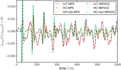
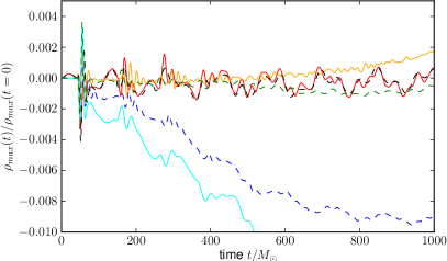
Evolutions of static star spacetimes are standard benchmarks for general-relativistic implementations, see e.g. Thierfelder et al. (2011a); Radice et al. (2014b). Here, before presenting BNS evolutions, we assess the convergence of the HO and HO-Hyb schemes for the star solution, compare different reconstruction procedures, and contrast the results with those obtained with the LLF second-order scheme. This benchmark allows one to study many features of generic neutron star evolution in a simple and controlled setup.

Our tests show that stable long-term evolutions of star spacetimes can be achieved with HO methods, but convergence is limited to second-order. For the WENOZ reconstruction, we shall show that the origin of the inaccuracy is related to the specific values of the WENO weights that are nonoptimal both in the bulk of the matter distribution and at the star surface. Thus, at typical resolutions for 3D runs, one does not expect an optimal convergence rate.

The star initial model is a $\Gamma=2$ polytrope with gravitational mass $M=1.400$, baryonic mass $M_{b}=1.506$ and central rest mass density $\rho_{c}=1.28\times 10^{-3}$. The BSSNOK evolution scheme is used for the metric evolution. We employ octant symmetry to reduce the computational costs.

The grid is composed of three fixed refinement levels. Simulations are performed with $n=(48,64,96,128)$ points covering the neutron star leading to a grid spacing of $h=(0.375,0.28125,0.1875,0.140625)$. It is ensured that the finest box covers the star entirely. Table 1 summarizes the simulations and settings. Note that for both the HO and HO-Hyb schemes, the MP5 reconstruction requires larger values of $f_{atm}$ and $f_{hyb}$ than the WENOZ one in order to achieve stable long-term evolutions.

At the continuum level the evolution of a static solution is trivial. Numerically, if a scheme allows long-term stable evolution, discretization errors trigger radial oscillations, which are observable, for example, in the central rest mass density. The oscillations are triggered by atmosphere effects and converge to 0 increasing the resolution. Figure 1 (top panel) shows the oscillations of the central rest mass ($\rho_{\max}$) density over a simulation time of about several radial periods for the polytropic EOS. We compare the LLF, HO, and HO-Hyb scheme for both WENOZ and MP5 reconstruction. The figure suggests that the HO scheme is slightly more accurate than the LLF for all the reconstructions considered, i.e. the amplitude of the oscillations is smaller.

The role of the star’s surface is illustrated by considering evolutions with the $\Gamma$-law EOS, bottom panel of Fig. 1. In our experience, truncation errors with such EOS are larger than the polytropic case with any numerical scheme, because significant unphysical shock-heating is observed at low-densities. Indeed, the $\rho_{\max}$ oscillations are larger than in the polytropic case. The best results for this test are obtained with the LLF-schemes and the HO-Hyb-WENOZ scheme. Moreover, the HO scheme gives by far the largest discrepancy to the initial configuration. This is due to the larger atmosphere threshold that have to be employed for stable simulations with the HO scheme, see Tab. 1.

Figure 2: Evolution of the $L_{1}$-distance $||\rho(t)-\rho(0)||_{1}$ for different numerical methods and resolution. Different resolutions are shown with different colors. The dashed colored lines are the same for the corresponding solid but scaled according to second-order convergence. Top: polytropic EOS. Bottom: $\Gamma$-law EOS.

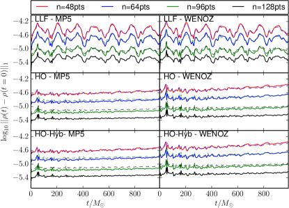
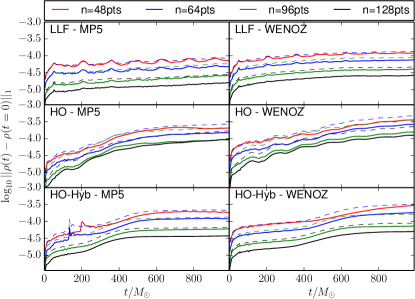
In order to verify the convergence rate of the scheme we consider the $L_{1}$ norm of the difference between the evolution profile and the initial data (exact solution). Figure 2 plots the $L_{1}$ distance from the exact solution for all resolutions and schemes for the polytropic (top) and $\Gamma$-law (bottom) EOS. Focusing on the top panel, we observe that the absolute error of the HO and HO-Hyb schemes is smaller and less oscillatory than that of the LLF. Also, the oscillation amplitude in the norm is smaller. The convergence rate of all the schemes is approximately second order (cf. dashed lines). The bottom panel shows that, at the same resolutions, the absolute errors in the $\Gamma$-law evolutions are approximately ten times larger. In this case, it is more difficult to maintain the initial equilibrium configuration. The larger deviations in the norms are not due to mass losses, but mainly to the deformation of the initial (exact) star profile due to truncation errors. In this test, the performances of the HO scheme are slightly worse than those of the LLF. The HO-Hyb algorithm gives results in-between the HO and the LLF-method. Again, for all the schemes, second-order convergence is observed.

Figure 3: Deviation from optimal WENOZ weights for the $\Gamma=2$ EOS spherical star. The plot shows the absolute difference with respect to optimal weights $d^{(k)\pm}_{j}$ of (13) for various projected fluxes $\hat{F}^{(k)\pm}$ and after a very short evolution time, $t\sim 0.003$. Note that, by symmetry, $d^{(2)\pm}_{j}=d^{(1)\pm}_{j}$ and $d^{(k)\pm}_{j}(x>0)=d^{(k)\mp}_{j}(x<0)$. For this test we evolve few Euler timesteps at a unigrid resolution of $h=0.15$, $n=128$, and CFL of $0.01$. The vertical line marks the star surface.

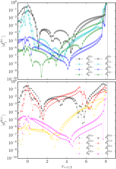
Why the nominal high-order convergence is not achieved in these tests? By considering the WENO weights for this problem, one finds that, at least at these resolutions, the weights are not optimal. Hence, the interpolation of the intercell-fluxes is affected by the lower-order component, and nominal convergence cannot be achieved. Figure 3 shows the absolute values of the differences

$$d^{(k)\pm}_{j}=\omega^{(k)\pm}_{j}-o_{j}$$ (13)

for $j=0,1$ (the third weight $j=2$ carries redundant information and it is not shown), where $\omega^{(k)\pm}_{j}$ are the weights associated to the reconstruction of the characteristic flux variables $\hat{F}^{(k)\pm}$. The $d_{j}$’s are computed in the $x$-direction and after a very short evolution time corresponding to few Euler timesteps. For optimal weights, one has $d_{j}=0$, and the algorithm locally achieves the formal fifth-order convergence. If $d_{j}\gg 0$ for some $j$, then the corresponding sub-stencil has a smaller weight in the reconstruction and the local convergence order is reduced. As shown in the figure, the weights significantly deviate from the optimal values both in the bulk of the star (notably at the center), and at the surface. A rigorous and complete analysis of the WENO weights on the star solution in 3D is difficult and beyond the purpose of this work. However, by inspecting the convergence properties of the weights in some given direction we observe that some of the necessary conditions for high-order convergence, namely $d^{(k)\pm}_{j}=\mathcal{O}(h^{2})$ and $\sum_{j}d^{(k)\pm}_{j}=\mathcal{O}(h^{6})$ Henrick et al. (2005), are not met.

V Binary Neutron Star Evolutions

Table 2: BNS quasicircular initial data. Columns: name, EOS, binary mass, rest mass, ADM mass, angular momentum, GW frequency. All configurations are equal-masses and irrotational.

Name	EOS	$M$	$M_{b}$	$M_{\rm ADM}$	$J_{0}$	$M\omega_{0}$
SLy135135_0060	SLy	2.700	2.989	2.671	6.872	0.060
SLy135135_0038	SLy	2.700	2.989	2.678	7.658	0.038
MS1b135135_0038	MS1b	2.700	2.935	2.678	7.665	0.038

Table 3: Grid configurations and summary of BNS runs. Columns: BNS configuration, shortname for grid configuration, refinement levels, minimum moving level index, number of points per direction in fixed levels, number of points per direction in moving levels, resolution per direction in the finest level $l=L-1$, number of points in radial direction in spherical patches, resolution per direction in the level $l=0$.

BNS	Grid								Numerical Flux Scheme
	Name	$L$	$l^{mv}$	$n$	$n^{mv}$	$h_{L-1}$	$n_{r}$	$h_{0}$	LLF		HO		HO-Hyb
									MP5	WENOZ	MP5	WENOZ	MP5	WENOZ
SLy135135_0060	Low (L)	7	2	128	64	0.228	128	14.592	$\checkmark$	$\checkmark$	$\checkmark$	$\checkmark$	$\checkmark$	$\checkmark$
	Med (M)	7	2	192	96	0.152	192	9.728	$\checkmark$	$\checkmark$	$\checkmark$	$\checkmark$	$\checkmark$	$\checkmark$
	Hig (H)	7	2	256	128	0.114	256	7.296	$\checkmark$	$\checkmark$	$\checkmark$	$\checkmark$	$\checkmark$	$\checkmark$
	Fin (F)	7	2	320	160	0.0912	320	5.8368	$\checkmark$	$\checkmark$	$\checkmark$	$\checkmark$	$\checkmark$	$\checkmark$
SLy135135_0038	Low (L)	7	2	160	64	0.228	-	14.592	$\times$	$\checkmark$	$\times$	$\times$	$\times$	$\checkmark$
	Med (M)	7	2	256	96	0.152	-	9.728	$\times$	$\checkmark$	$\times$	$\times$	$\times$	$\checkmark$
	Hig (H)	7	2	320	128	0.114	-	7.296	$\times$	$\checkmark$	$\times$	$\times$	$\times$	$\checkmark$
	Fin (F)	7	2	400	160	0.0912	-	5.8368	$\times$	$\times$	$\times$	$\times$	$\times$	$\checkmark$
MS1b135135_0038	Low (L)	7	2	128	80	0.291	-	18.624	$\times$	$\checkmark$	$\times$	$\times$	$\times$	$\checkmark$
	Med (M)	7	2	192	120	0.21825	-	12.416	$\times$	$\checkmark$	$\times$	$\times$	$\times$	$\checkmark$
	Hig (H)	7	2	256	160	0.1455	-	9.312	$\times$	$\checkmark$	$\times$	$\times$	$\times$	$\checkmark$
	Fin (F)	7	2	320	200	0.1164	-	7.4496	$\times$	$\times$	$\times$	$\times$	$\times$	$\checkmark$

V.1 Initial configurations and grid setups

Initial data for our simulations are conformally-flat BNS irrotational configurations in quasicircular orbits computed with the Lorene library Gourgoulhon et al. (2001). They are characterized by the Arnowitt-Deser-Misner (ADM) mass-energy $M_{\text{ADM}}$, the angular momentum $J_{0}$, baryonic or rest mass $M_{b}$, and the mass-rescaled and dimensionless GW circular frequency $M\omega_{0}$. The relevant properties are summarized in Tab. 2. SLy135135_0060 is described by the SLy EOS and is prepared at about three orbits to merger. SLy135135_0038 is a similar configuration at about 10 orbits to merger. MS1b135135_0038 is described by the MS1b EOS, and has same initial frequency of SLy135135_0038.

We present a total of 32 new evolutions of these initial data. SLy135135_0060 has been evolved with LLF, HO, and HO-Hyb numerical fluxes, each combined with WENOZ and MP5 reconstructions. For each flux and reconstruction combination, four different grid resolutions were considered. The grid specifications for all the runs are reported in Tab. 3. The four grid resolutions allow us to perform self-convergence tests by choosing differently resolved triplets of data. We analyze two different triplets with $n^{mv}=(64,96,128)$ and $n^{mv}=(96,128,160)$ chosen such that the differences in the three resolutions are nearly optimal Bernuzzi et al. (2012a). SLy135135_0038 and MS1b135135_0038 have been evolved only with the HO-Hyb-WENOZ scheme, but we evolved the same data with the LLF-WENOZ in Bernuzzi et al. (2015). Note also that the runs *_0038 with HO-Hyb-WENOZ were evolved without spherical patches, i.e. using a computationally less expensive setup. Atmosphere parameters are $f_{atm}=10^{-11}$, $f_{thr}=10^{2}$, $f_{hyb}=10^{2}$.

During the development of this work we tested the robustness of our findings by further varying i) grid setups, ii) the formulation for the metric equations, and iii) BNS configurations. In particular, we performed additional convergence tests with a grid setup employing neither moving boxes nor spherical patches (cf. Radice et al. (2014b)) evolving SLy135135_0060 with LLF-WENOZ and HO-WENOZ and using BSSNOK. Other convergence tests were performed with the $\Gamma$-law EOS configuration previously used in Thierfelder et al. (2011a); Hilditch et al. (2013). In the following, we do not discuss these tests but focus on the most detailed and representative simulations of Tab. 3. All our results are consistent with the findings reported in the following. We expect our findings will carry over in the computation of inspiral-merger waveforms with the broad range of EOS typically employed for GW modeling (e.g. Bernuzzi et al. (2015)) and for approximately equal masses BNS.

V.2 Conserved quantities

Figure 4: SLy135135_0060: $L_{2}$ norm of the Hamiltonian constraint on refinement level $l=1$ for different grid resolution and numerical schemes. Dashed lines show results scaled to second-order.

Figure 5: SLy135135_0060: ADM energy Eq. (14) extracted at coordinate sphere $r=450$ for different grid resolution and numerical schemes. Dashed lines show results scaled to second-order.

Figure 6: SLy135135_0060: rest mass conservation $\log_{10}\left(\left|M_{b}(t)/M_{b}(t=0)\right|\right)$ and its convergence on refinement level $l=5$ for different grid resolution and numerical schemes. Dashed lines show results scaled to fourth-order; which is the order of the restriction operator (see text).

Figure 7: Conserved quantities for SLy135135_0038 with the HO-Hyb-WENOZ scheme. Top panel: conservation of the baryonic mass measures on level $l=4$. Dashed lines correspond to an assumed fourth order convergence, cf. Fig. 6. Middle panel: $L_{2}$-volume norm of the Hamiltonian constraint measured on level $l=1$. Dashed lines correspond to an assumed second-order convergence, cf. Fig. 4. Bottom panel: Self-convergence of the ADM-energy, where we have not corrected the energy by the emitted GW energy. The energies are extracted at $r=1000M_{\odot}$. Dashed lines correspond to an assumed second-order convergence, cf. Fig. 5.

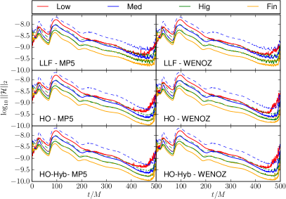
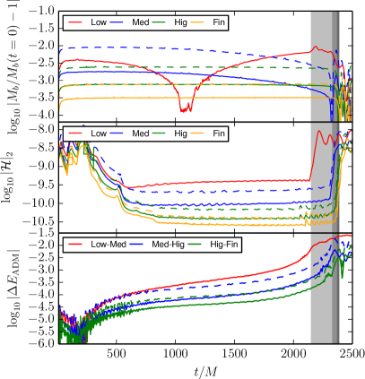
Conserved quantities are fundamental diagnostics for evaluating the performance of a numerical scheme. Before discussing the waveform accuracy we discuss the convergence properties of these quantities. During the BNS evolution we choose to monitor the following three quantities.

(1) The $L_{2}$ norm of the Hamiltonian constraint, $||\mathcal{H}||_{2}$, see e.g. Hilditch et al. (2013) for the definition of $\mathcal{H}$. In the continuum limit $\mathcal{H}\to 0$, any numerical solution must show convergence to zero in order to be consistent with Einstein equations.

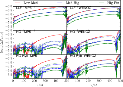
(2) The ADM mass of the spacetime. In asymptotically flat spacetimes, one can define the conserved ADM mass as $M_{\rm ADM}=\lim_{r\to\infty}E_{\rm ADM}(r)$, where

$$E_{\rm ADM}(r)=\int_{S_{r}}ds_{l}\sqrt{\gamma}\,\gamma_{ij}\gamma^{kl}\left(\gamma_{ik,j}-\gamma_{ij,k}\right)$$ (14)

is computed on a coordinate spheres $S_{r}$ of radius $r$ in the wave zone, and $\gamma_{ij}$ is the spatial metric. $E_{\rm ADM}(r)$ is expected to deviate from $M_{\rm ADM}$ due to the gravitational energy radiated away from the sphere, $E_{\text{GW}}$. Conservation at large finite $r$ is expected for the quantity $M_{\rm ADM}^{(r)}=E_{\rm ADM}(r)+E_{\text{GW}}(r)\approx M_{\rm ADM}$.

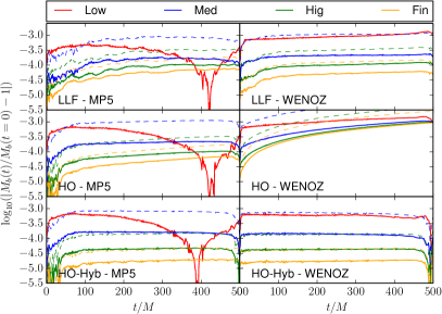
(3) The rest mass of the matter,

$$M_{b}=\int d^{3}x\sqrt{\gamma}D$$ (15)

whose conservation follows from the first component of (1), see e.g. Font (2007); Dietrich et al. (2015). In case (1) are solved on a single grid, $M_{b}$ is preserved at round-off error; violations at the truncation error level are, however, generically expected in cases in which adaptive mesh refinement is employed Dietrich et al. (2015).

We first discuss the conservation and convergence of these quantities in the SLy135135_0060 evolutions for different numerical schemes and resolutions, then consider the same quantities for the longer runs.

V.2.1 SLy135135_0060: Hamiltonian constraint

The $L_{2}$ norm of the Hamiltonian constraint computed on level $l=1$ is shown in Fig. 4. During the inspiral-merger the norm is decreasing because of the constraint propagation and damping properties of the Z4c evolution scheme Weyhausen et al. (2012). The violation of the constraint is of the order $\sim 10^{-9}$ and shows 2nd order convergence to round off at increasing grid resolution (cf. dashed lines). Note that constraint violations stay below the initial value. We observe no significant difference between the different reconstruction and flux computation routines.

V.2.2 SLy135135_0060: ADM energy

The convergence of $E_{\rm ADM}$ at increasing grid resolutions is shown in Fig. 5. WENO-based schemes achieve clean second-order convergence up to the moment of merger. The use of high-order schemes for the numerical fluxes results in smaller absolute differences between one resolution and the other, thus indicating a better accuracy. By contrast, the combination of high-order schemes and MP5 reconstruction performs worse. Although, MP5 gives smaller differences for high resolutions, one does not see a clear convergence order, and the Low (L) grid is not in the convergent regime.

Overall, the relative accuracy of $E_{\rm ADM}$ for the grid F is of the order of $10^{-3}-10^{-4}$. That accuracy is signifcantly smaller than the GW energy emitted $E_{\rm GW}(r)$ only towards the merger moment, where $E_{\rm GW}(r)$ reaches few percent Bernuzzi et al. (2016). As a consequence, the convergence properties of the complete quantity $M_{\rm ADM}^{(r)}$ are slightly worse and, as with high-order methods, it remains difficult to properly resolve $M_{\rm ADM}^{(r)}$.

Both $\mathcal{H}$ and $E_{\rm ADM}$ data show that the truncation error scales at second-order at the considered resolutions. Motivated by the analysis of Sec. IV, we have inspected the WENO weights also for the binary case. The quantities $d^{(k)\pm}_{i}$ for the stars in the binary are qualitatively similar, at early times, to the single star case. The HO schemes fail to achieve the nominal high-order convergence both in the bulk of the matter and at the surface. We conclude that high-order convergence cannot be expected at these resolutions.

V.2.3 SLy135135_0060: Rest Mass

Let us discuss rest mass conservation. In neutron star simulations the conservation of rest mass is affected by three dominant errors: (i) the artificial atmosphere, (ii) the restriction operation, and (iii) refinement boundaries. Because of our particular grid choice no significant rest mass crosses the finest refinement level during the inspiral and merger. When the two boxes of the finest refinement level touch each other, BAM regrids and a larger box covering the strong-field region is created. Thus, we expect that artificial atmosphere and restriction are the main source of uncertainty in Eq. (15). Of course, the situation is different in the subsequent postmerger and collapse phase in which the rest mass spread all over the grid and the particular choice of slicing leads to an apparent loss of rest mass when the singularity forms Thierfelder et al. (2011b); Dietrich and Bernuzzi (2015). In this paper, we focus on the inspiral-merger and do not discuss these issues. The artificial atmosphere treatment typically introduces a $\mathcal{O}(h^{2})$ error in $M_{b}$ that is characterized by mass losses, see Dietrich et al. (2015). Note that an error localized around the star surface can become negligible for the volume integral (15) at sufficiently high resolutions. The restriction operation and regridding from the finer levels to coarser ones are performed in this work with a fourth-order WENO algorithm. Thus, a $\mathcal{O}(h^{4})$ error is expected at best.

The rest mass conservation is monitored by the relative error $\left|M_{b}(t)/M_{b}(0)\right|$, where $M_{b}(t=0)$ is computed after interpolation of the initial data on the BAM grid and after restriction of the data from finer to coarser levels. The evolution of the error is shown in Fig. 6. For any reconstruction choice, the HO schemes perform significantly worse than the LLF or HO-Hyb schemes. This is most likely due to a lack of accuracy in the resolution of the low-density flow, caused by the particularly large values of $f_{atm}$ necessary to stabilize these simulations. This effect is observed also in the single star evolutions of Sec. IV, although we have not discussed this explicitly there. At the lowest resolution the use of MP5 reconstruction produces serious violations of $M_{b}$ (red lines, right panels). A convergence order $\sim 4$ is observed in the LLF-WENOZ runs at early times; for $t\gtrsim 100M$ the convergence of the error is slower and dominated by the $\mathcal{O}(h^{2})$ component. The best conservation is obtained with the HO-Hyb flux scheme employing the WENOZ reconstruction. In these simulations the dominant error is given by the truncation error $\mathcal{O}(h^{4})$ of the restriction operator over the whole simulated time.

V.2.4 SLy135135_0038 and MS1b135135_0038

The analysis presented for the SLy135135_0060 evolutions holds qualitatively also for the longer and more challenging 10 orbits simulations, although we find that for such long simulations higher resolutions are needed to obtain the same accuracy. In particular, overconvergence is observed in one triplet and it is due to the lowest resolution simulations.

Conserved quantities are shown in Fig. 7 for SLy135135_0038. The upper panel shows the rest mass conservation. In contrast to SLy135135_0060, the two lowest resolutions do not show a clear convergence order. The error grows up to 1% on level $l=4$. For the two highest resolutions fourth order convergence, which is again caused by the restriction operation, is observed. For the highest resolution the error stays during the entire inspiral below the 0.05% level within level $l=4$. The error even decreases significantly when computing the mass on level $l=5$ and becomes smaller than $10^{-5}$ for the highest resolution. This shows that, for the considered levels, the restriction operation is the dominant error contribution for the two highest resolutions and supports our argumentation for SLy135135_0060.

The middle panel of Fig. 7 presents the evolution of the $L_{2}$-volume norm of the Hamiltonian constraint. As for SLy135135_0060, the constraints stay below the initial value during the entire inspiral up to the moment of merger. second-order convergence is recovered for the two highest resolutions, cf. dashed lines.

The bottom panel of Fig. 7 shows a self-convergence test of the ADM-energy extracted at $r=1000M_{\odot}$. The dashed lines correspond to second-order convergence, which is obtained for the two highest resolutions, but not for the lower resolution. The triplet (L,M,H) shows overconvergence due to the Low (L) resolution simulation.

V.3 Waveform convergence

Figure 8: Top: $\ell=m=2$ waveforms for SLy135135_0060 from runs with grid Low and varying the numerical scheme. The vertical line marks the moment of merger for the LLF simulation. Middle: Phase differences between HO-Hyb and LLF simulations employing WENOZ reconstruction and with the same grid resolutions. Bottom: Phase differences between HO-Hyb simulations employing WENOZ and MP5 reconstruction with the same grid resolution.

Figure 9: Convergence of SLy135135_006. The different panels show the phase differences in log scale for different reconstructions: MP5 (left) and WENOZ (right). The algorithms from top to bottom are: LLF, HO, HO-Hyb. The vertical shaded regions represent the moment of merger for different resolutions: light gray for $[u_{\rm mrg}^{\rm L},u_{\rm mrg}^{\rm M}]$, gray for $[u_{\rm mrg}^{\rm M},u_{\rm mrg}^{\rm H}]$ and dark gray for $[u_{\rm mrg}^{\rm H},u_{\rm mrg}^{\rm F}]$. To show convergence we rescale the phase differences assuming second-order convergence, cf. dashed and dot-dashed lines.

In this section we discuss the convergence of the GWs. We focus on the GW phase that is the main quantity of interest for GW modeling. A major goal for NR simulation is to control phase uncertainty and assign precise error bars to this quantity.

The emitted GWs are calculated by computing the Weyl $\Psi_{4}$ scalar on coordinate spheres of radius $r$ in the wave zone. As customary, we work with the spin weighted spherical harmonics projections (independent of the viewing angle), reconstruct the GW multipolar modes $h_{\ell m}$ from $\Psi_{4}$ projections by solving $\ddot{h}_{\ell m}=\psi_{\ell m}$ in the frequency domain Reisswig and Pollney (2011), and focus on the dominant mode $\ell=m=2$. Amplitude and phase are defined as

$$r\,h_{22}=A_{22}\ e^{-i\phi_{22}}\ .$$ (16)

Waveforms are shown against the retarded time

$$u=t-r_{*}=t-r-2M\log\left(\frac{r}{2M}-1\right)\ .$$ (17)

The moment of merger $u_{\text{mrg}}$ is defined as the time of the first peak of $A_{22}$, and conventionally marks the end of the inspiral Bernuzzi et al. (2014).

V.3.1 SLy135135_0060

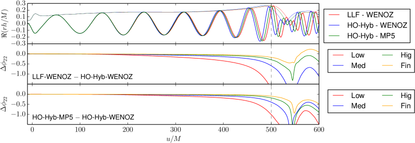
Figure 8 show the real part of the SLy135135_0060 waveform at the lowest resolution for different numerical schemes (top panel) and the phase difference obtained using different numerical schemes and the same resolutions. The vertical line marks $u_{\text{mrg}}\sim 500M$ for the data of grid Low. The phase differences of waveforms computed with different numerical scheme decrease as resolution increases, indicating that all schemes converge to the same continuum, physical solution. At $u_{\text{mrg}}$ the phase differences are largest. The differences between HO-Hyb and LLF (both with WENOZ reconstruction) at the lowest resolutions are $\Delta\phi\sim-2$ rad, and reduce to $\Delta\phi\sim-0.15$ rad at the highest resolution. The differences between HO-Hyb-MP5 and HO-Hyb-WENOZ at the lowest resolutions are $\Delta\phi\sim-1$ rad, and reduce to $\Delta\phi\sim-0.1$ rad at the highest resolution. The difference between HO-WENOZ and HO-Hyb-WENOZ at the lowest resolution is of the order $\Delta\phi\sim-0.5$ rad, and it reduces to $\Delta\phi\sim-0.25$ rad at the highest resolution (not shown in the figure).

Figure 10: Phase error budget of SLy135135_0060 with the HO-Hyb-WENOZ scheme. Solid lines are phase differences between runs at different resolutions; dashed lines are differences with the Richardson extrapolated data; dashed dotted lines are differences between phase extracted at finite radii and the radius-extrapolated one.

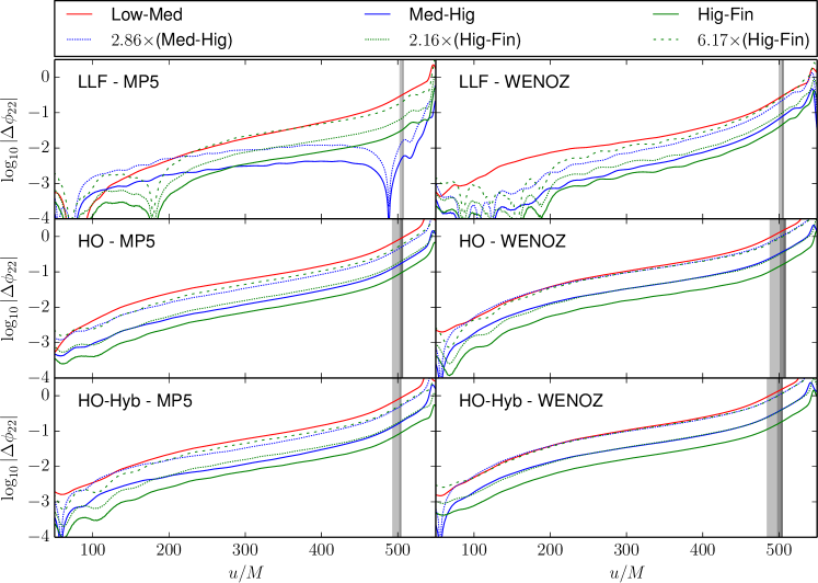
A three-level self-convergence study for SLy135135_0060 is shown in Fig. 9 for all the numerical schemes considered. As mentioned above, performing the analysis with four instead of three different resolutions allows one to robustly assess convergence. The latter is, in fact, evaluated for two triplets. All our convergence plots show both the differences between the data (solid lines) and those scaled assuming second-order convergence (dotted and dashed lines). Note that, in all our simulations, the phase is overestimated (faster) at low resolutions as a result of numerical dissipation Bernuzzi et al. (2012b).

Independently on the reconstruction method, the LLF scheme shows larger oscillations and a more complicated behavior than the corresponding HO and HO-Hyb simulations. The convergence properties of LLF-MP5 data are not systematic and a zero crossing in $\Delta\phi$ is visible before $u_{\text{mrg}}$. These LLF-MP5 data are not in convergence regime and are unreliable for producing an error budget. The LLF-WENOZ data improve on this situation. With the LLF-WENOZ setup we observe a convergence order slightly higher than second-order in the triplet (L,M,H), and slightly below second-order in the triplet (M,H,F). That indicates that the resolution $n=64$ is too low and should be discarded; only (M,H,F) should be considered. Still, it is difficult to obtain a precise error estimate using only the (M,H,F) triplet because one does not know how robust is the convergence result at higher resolutions Bernuzzi et al. (2012a). Another resolution is desirable; in the absence of that, the differences between the two highest resolutions can be taken as an error estimate Bernuzzi et al. (2015).

The HO and HO-Hyb schemes employing the MP5 reconstruction show a convergence order of $\sim 3$ at low resolutions -(L,M,H) triplets-, but a lower convergence order of $\sim 2$ (or slightly below) at higher resolutions, (M,H,F,) triplet. The MP5 high-order fluxes improve significantly over the LLF ones. However, without a fifth resolution, it is impossible to make a robust claim about convergence.

Contrary to the other setups, the HO and HO-Hyb WENOZ schemes show a very robust convergence behavior. We observe clean second-order convergence for all four resolutions. This convergence order is also consistent with what we observe in single star evolution and in the conserved quantities discussed above. From the analysis of the phasing solely one cannot clearly point out differences between the HO and HO-Hyb schemes. However, combining all the results (cf. Fig. 2 and Fig. 6), we conclude that the HO-Hyb-WENOZ scheme performs better among those we tested and at the resolutions explored here.

Let us mention that the plot also shows that the differences between different resolutions are smaller for LLF simulations than the HO or HO-Hyb ones. This fact can be interpreted as the LLF having smaller absolute errors, i.e. begin more accurate for lower resolutions, although the interpretation is not straightforward in the absence of clear convergence.

V.3.2 SLy135135_0038 and MS1b135135_0038

Figure 11: Phase convergence of MS1b135135_0038 (upper panel) and SLy135135_0038 (lower panel) with the HO-Hyb-WENOZ scheme.

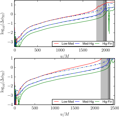
Self-convergence studies for the phase evolution of SLy135135_0038 and MS1b135135_0038 are shown in Fig. 11 for the HO-Hyb-WENOZ scheme. Also in these long runs numerical dissipation artificially accelerates the phase evolution. The convergence behaviour is similar to the SLy135135_0060 case, although in these long runs the lowest resolution $h\sim 0.23$ ($n^{mv}=64$) does not give convergence results for $u\gtrsim 1000M$ (SLy) and $u\gtrsim 1500M$ (MS1b). At late times, we observe instead overconvergence due to the Low-grid simulation. As a consequence, the lowest resolution runs should not be used for producing the error budget. The phase differences accumulated to $u_{\text{mrg}}$ between H and F-runs are about $\Delta\phi\sim 1$ rad. They are about a factor 10 larger than in the shorter runs.

VI Radius extrapolation

Figure 12: SLy135135_0060 finite radius extraction uncertainty (HO-Hyb-WENOZ scheme). Top panel shows the phase difference for different extraction radii computed to the polynomial extrapolation with $K=2$ (solid lines). The dashed lines show the difference the extrapolated waves with $K=1,3$ and the last radius $r_{N}=1100$ as well as the difference between the $K=2$ and NLO extrapolation. Bottom shows the phase difference between the NLO extrapolated value and finite radii extracted data (solid lines). Dashed lines show the difference between the NLO extrapolation for different radii and the $K=2$ extrapolated one.

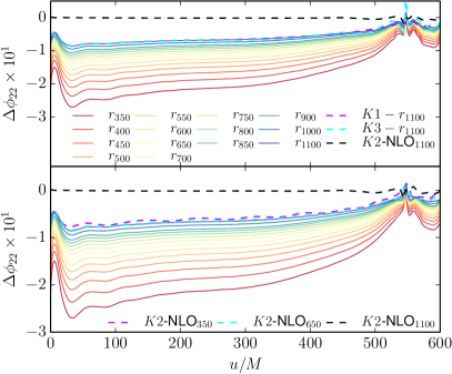
The waveform error budget must take into account also the effect of finite-radius extraction. As we see, the latter uncertainty is non-negligible and comparable to the truncation error. It can be evaluated by extrapolating the waveform in radius e.g. Boyle et al. (2007); Bernuzzi et al. (2012a); Lousto et al. (2010). Notably, the finite-extraction-radius uncertainty on the phase has opposite sign than the truncation error uncertainty: the phase evolution is faster for waveforms extracted at larger radii.

Two extrapolation methods are considered here. In the first, the waveform is evaluated at different radii $r_{j}$ with $j=0...N$ and phase and amplitude are extrapolated using a polymomial of order $K<N$,

$$f(u;r_{j})=f_{0}(u)+\sum^{K}_{k=1}f_{k}(u)r^{-k}_{j}\ .$$ (18)

In the second method, one considers the next-to-leading-order (NLO) behaviour in $r$ of the $\Psi_{4}$ multipoles Lousto et al. (2010),

$$r\,\psi_{\ell m}=r\,\ddot{h}_{\ell m}+\frac{\ell(\ell+1)}{2r}\;r\,\dot{h}_{\ell m}+\mathcal{O}(r^{-2})\ ,$$ (19)

and obtains an extrapolation formula for $r\,\ddot{h}_{\ell m}$ that uses $\psi_{\ell m}$ extracted at a given radius . The extrapolated $r\,h_{\ell m}$ is then reconstructed from $r\,\ddot{h}_{\ell m}$.

Figure 12 compares the differences between the extrapolated quantities and the finite-radii ones for SLy135135_0060 (again, we work with the best data HO-Hyb-WENOZ). The polynomial extrapolation (18) requires a choice for $K$, but the phase extrapolation is rather insensitive on the choices $K=1,2,3$. Considering the difference between the extrapolated and the last radius ($r_{N}=1100$), one can assign an uncertainty to the extrapolate phase. The uncertainty is larger at early times (lower GW frequencies), $\delta\phi\sim 0.1$, and monotonically decreases toward the moment of merger to $\delta\phi\sim 0.05$ The fact that the finite-radius uncertainty is larger at lower frequencies is clear from Eq. (19): taking the double integral of both sides in order to obtain the metric waveform, and considering a signal at frequency $\omega$, the second term $\propto 1/r$ gets a factor $1/\omega$ from the integral of the metric waveform Lousto et al. (2010).

Figure 12 also compares the polynomial extrapolation with the second method outlined above. We use (19) for radii $r=350$, $650$ and $r=r_{N}$. We find the results are compatible with those of the polynomial extrapolation. The difference between the extrapolated phases with (18) and (19) is significantly smaller than the finite radius extraction uncertainty assigned above. Moreover, the formula (19) is rather robust for the phase extrapolation; the use of $r=350$ is already comparable with the polynomially extrapolated phase.

We find similar results for the extrapolation of the amplitude (not shown in the figure). The only difference is that the amplitude radius-extrapolation is slightly more sensitive to $K$ and stability can be achieved for $K=2,3$. The uncertainty of the extrapolated amplitude ($K=2$) is about $0.2\%$ and has smaller variation in time than the phase.

VII Waveform Error Budget

In this section we discuss the error budget on the waveforms generated with the high-order WENO algorithm. We work with the best data HO-Hyb-WENOZ, for which we have a clear convergence assessment, and include the finite-extraction-radius uncertainties discussed above.

For any finite-differencing algorithm, the value of a quantity $f^{(h)}$ computed at resolution $h$ can be written as

$$f^{(h)}=f^{(e)}+\sum^{\infty}_{i=p}A_{i}h^{i}\ ,$$ (20)

where $f^{(e)}$ is the exact, continuum value obtained for $h\to 0$, and $p$ the convergence order. The quantities $A_{i}$ are not necessarily small and might depend on the number of floating point operations. Although it is not possible to compute $f^{(e)}$, one can use the set of data at different resolutions to improve the simulation results. A way to proceed is to consider the Richardson extrapolation method. The latter is a simple algorithm that, given (i) a dataset $(f^{(h)})$ at different finite resolutions and (ii) an accurate measure of the convergence order $p$, allows one to generate a better approximation to $f^{(e)}$ Richardson (1911). The Richardson extrapolated value is indicated as $\mathcal{R}[(f^{(h)})]$. This method has already been used for estimating waveform errorbars in e.g. Bernuzzi et al. (2012a); Hinder et al. (2013); Radice et al. (2015). Here we are particularly interested in the robustness/stability of the extrapolation using different datasets. An alternative resolution extrapolation method proposed in the literature is studied in Appendix B.

In the following, we consider the Richardson extrapolation of different time series: $\mathcal{R}[(L,M,H)]$, $\mathcal{R}[(M,H,F)]$, and $\mathcal{R}[(L,M,H,F)]$, where L stands for grid Low, M for grid Med, and so on. We investigate whether the different $\mathcal{R}[.]$ are consistent. The extrapolated time series can then be used as best data, i.e. an improved approximation of $f^{(e)}$. A measure of the uncertainty to be assigned to this best approximation is the difference with the highest resolution (F) or with another extrapolation.

VII.1 SLy135135_0060

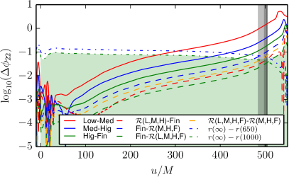
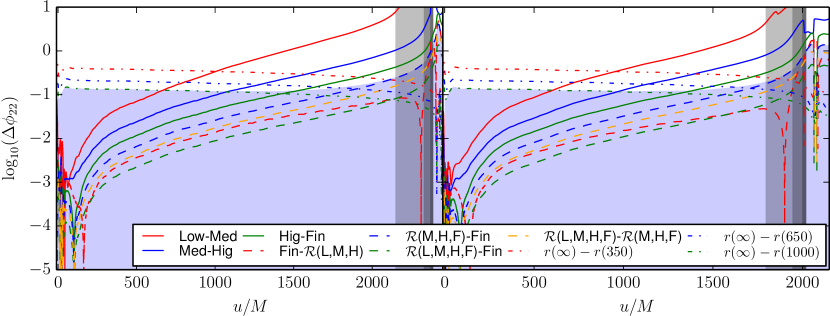
Figure 10 shows the waveform phase differences for SLy135135_0060 (solid lines) and the differences between the extrapolated time series and data at grid F (dashed lines). The extrapolation $\mathcal{R}[(L,M,H)]$ is rather effective in improving the approximation: it is very close to the phase computed with grid $F$, although it overestimates the latter. The positive phase difference $\Delta\phi(H-\mathcal{R}[(L,M,H)])$ is larger than $\Delta\phi(F-\mathcal{R}[(L,M,H,F)])$, suggesting a convergent behaviour. $\mathcal{R}[(L,M,H,F)]$ estimates a slower phase than $F$. $\mathcal{R}[(M,H,F)]$ estimates a slower phase than both $F$ and $\mathcal{R}[(L,M,H,F)]$, but the extrapolation might be more biased by the use of three resolutions instead of four. The positive differences $\Delta\phi(F-\mathcal{R}[(M,H,F)])$ are slightly smaller than the positive $\Delta\phi(\mathcal{R}[(L,M,H,F)]-\mathcal{R}[(M,H,F)])$. Although not shown in the figure, we verified that the Richardson extrapolation that uses only two datasets is not robust; the result depends heavily on the choice of the pair of the datasets and extrapolation results are incompatible with each other. We recommend the use of at least three, and possibly four, datasets at well-separated resolutions.

These results indicate that the extrapolations are robust. We choose $\mathcal{R}[(L,M,H,F)]$ as best data. The uncertainty of the best data can be assigned either as $\delta\phi=\Delta\phi(F-\mathcal{R}[(L,M,H,F)])$ or as $\delta\phi=\Delta\phi(\mathcal{R}[(L,M,H,F)]-\mathcal{R}[(M,H,F)])$. The former choice gives the smallest error bars, and is incompatible with the $\mathcal{R}[(M,H,F)]$. The latter choice instead assume the three-resolutions extrapolation $\mathcal{R}[(M,H,F)]$ is robust and assigns a slightly more conservative error bar.

The total error budget of SLy135135_0060 is reported in Fig. 10. The best approximation to the continuum data is given by $\mathcal{R}[(L,M,H,F)]$, with the uncertainty due to truncation error calculated as $\delta\phi_{(h)}=\Delta\phi(\mathcal{R}[(L,M,H,F)]-\mathcal{R}[(M,H,F)])$ as discussed above. The uncertainty $\delta\phi_{(r)}$ due to finite radius is instead computed as described above using the polynomial extrapolation with $K=2$ and last radius $r=1000$. The total error bar is computed as $\delta\phi=(\delta\phi_{(h)}^{2}+\delta\phi_{(r)}^{2})^{1/2}$ and shown as a shaded area.

The use of the HO-Hyb-WENO scheme at these resolutions, combined with the two extrapolation techniques described above, gives maximum phase uncertainties $\delta\phi_{(h)}\lesssim 0.05$ rad for $u\leq u_{\text{mrg}}$. The error budget is essentially flat at the level $\delta\phi\sim\delta\phi_{(r)}\lesssim 0.1$ rad, and dominated by finite-extraction errors (compare with Bernuzzi et al. (2012a)).

Figure 13: Phase error budget of SLy135135_0038 (left) and MS1b135135_0038 (right) similar to Fig. 10. Solid lines are phase differences between runs at different resolutions; dashed lines are differences with the Richardson extrapolated data; dashed dotted lines are differences between phase extracted at finite radii and the radius-extrapolated one. The conservative error estimate described in the text is given by the blue shaded region.

VII.2 SLy135135_0038 and MS1b135135_0038

The error budgets for SLy135135_0038 and MS1b135135_0038 are computed in the same way as above. The results are shown in Fig. 13, and focus on the simulations with the HO-Hyb-WENOZ scheme. In these long runs, the finite-radius uncertainties are essentially the same as those discussed for SLy135135_0060. From Fig. 13 one observes that $\delta\phi_{(r)}\lesssim 0.1$ rad and slightly decreases towards merger. The error bar is dominated by these finite-extraction errors at early times, $u\lesssim 1500~{}M$ for MS1b135135_0038 and $u\lesssim 1750~{}M$ for SLy135135_0038. The main difference with respect to SLy135135_0060 is related to the truncation error, and it is discussed below.

Considering the Richardson extrapolations, we find that the extrapolations $\mathcal{R}[(L,M,H)]$ and $\mathcal{R}[(L,M,H,F)]$ are effective and rather close to the data of grid $F$ (overestimating and underestimating the latter, respectively). Again, the positive difference $\Delta\phi=H-\mathcal{R}[(L,M,H)]$ is larger than the differences $\Delta\phi=\mathcal{R}[(L,M,H)]-F$ and $\Delta\phi=F-\mathcal{R}[(L,M,H,F)]$, possibly indicating a convergent behaviour of the extrapolation. However, the difference $\Delta\phi=\mathcal{R}[(L,M,H)-F]$ shows a zero crossing close to $u_{\text{mrg}}$ ($F$ data), likely due to the very different merger time in the $L$ data with respect to other datasets. The zero-crossing is not there in the difference $\Delta\phi=F-\mathcal{R}[(L,M,H,F)]$, which is also the smallest difference between grid $F$ and the various extrapolated data. The positive difference $\Delta\phi=F-\mathcal{R}[(M,H,F)]$ is instead larger than the differences with the extrapolations that include the grid $L$. Because the $L$ data show overconvergence at late time, a conservative choice for our best data and uncertainty is $\mathcal{R}[(M,H,F)]$ and $\delta_{(h)}\phi=F-\mathcal{R}[(M,H,F)]$. With this choice we find that truncation errors dominate the error budget at $u\gtrsim 1500~{}M$, i.e. during the last $5.5$ GW cycles, for MS1b135135_0038 and $u\gtrsim 1750~{}M$, i.e. during the last $7$ GW cycles, for SLy135135_0038. The maximum error is reached at $u_{\text{mrg}}$ and $\delta\phi_{(h)}\sim 1$ rad. A more optimistic choice, though not fully reliable based on the convergence result, is $\delta_{(h)}\phi=\mathcal{R}[(L,M,H,F)-\mathcal{R}[(M,H,F)]$ which leads to a maximum uncertainty of $\delta\phi_{(h)}\sim 0.7-0.9$ rad.

Finally, we compare the new HO-Hyb-WENOZ extrapolated waveforms with our previous simulations employing the LLF Bernuzzi et al. (2015). For SLy135135_0038 we find that the difference $\Delta\phi=\phi({\rm LLF-WENOZ})-\phi({\rm HO-Hyb-WENOZ})\sim-1$ rad at $u_{\text{mrg}}$, and is thus compatible with the error bar of the HO-Hyb-WENOZ. For MS1b135135_0038 $\Delta\phi=\phi({\rm LLF-WENOZ})-\phi({\rm HO-Hyb-WENOZ})\sim+1.2$ rad at $u_{\text{mrg}}$, which is compatible with the error bar assigned to the HO-Hyb-WENOZ and to the LLF data. In this case, the use of HO-Hyb-WENOZ reduces by about a factor 3 the error estimated on the phase.

VIII Summary

We explored the use of finite-differencing high-order WENO schemes in BNS inspiral-merger simulations, and compared those results with a second-order (LLF) scheme employing the same reconstruction methods. Simulations were performed at typical resolutions of the 3D grid. Our findings are summarised in the following.

(i) WENO methods are robust for these simulations; best results are obtained with the HO-Hyb-WENOZ scheme which significantly improves over the LLF, see e.g. Fig. 9. The HO-Hyb-WENOZ scheme allows us to consistently measure self-convergence in all the different datasets (triplets); and, hence, to robustly build an error budget by extrapolating consistently the finite-resolution datasets;

(ii) At the considered resolutions, the high-order convergence rate cannot be obtained due to nonoptimal values of the WENO weights. We experimentally observe that truncation errors scale at second-order rate for both single star and binary spacetimes. We do not align waveforms in time and/or phase in these analysis. In three orbits simulations (SLy135135_0060), convergence is observed by resolving the NSs with $\sim 64^{3}$ grid points. In ten orbits simulations, convergence is observed by resolving the NSs with at least $\sim 96^{3}$ grid points;

(iii) The HO-Hyb-WENOZ scheme combined with the Richardson extrapolation allows one to compute a robust error budget. Notably, our error budget procedure does not involve waveform alignment. The error budget for the three orbits runs (SLy135135_0060) is dominated by finite-extraction uncertainties, see Fig. 10. The overall phase uncertainty accumulated to merger ($u=u_{\text{mrg}}$) is below $0.1$ rad. The error budget of $\sim$ ten orbits runs is dominated by truncation error during the last 3-4 orbits; the phase uncertainty grows from $0.1$ to a maximum of $\sim 1$ rad at merger, see Fig. 13;

(iv) Comparing our results with Radice et al. (2014a, 2015, 2016), we find that, overall, our conclusions are in line with previous work. Common features are the following: the robustness of the high-order finite differecing scheme, the fact that the formal high-order accuracy is not achieved, and the magnitude of the phase uncertainties. the main differences are the performances of the MP5 reconstruction and the observed convergence order ($\sim 3$ instead of $2$). Both differences might be due to the use of different basic flux formula in the HO algorithm (the Roe solver instead of the LLF) and/or other implementation details, notably the use of positivity preserving limiters and the atmosphere treatment Radice et al. (2014b). Future work on the BAM code could be devoted to design improved and specific WENO weights for the problem.

We conclude that our high-order WENO implementation can be efficiently used for high-quality waveform production, and in future large-scale investigations of the binary parameter space. The computational cost for a $\sim 10$ orbit simulation composed of four resolutions is about $\sim 650$k core hours. We expect that the maximum phase uncertainty can be further reduced below $\delta\phi\lesssim 0.5$ rad by simulating an additional resolution at $\sim 192^{3}$ grid points. Using these resolutions, the BAM’s parallel efficiency is $\sim 80\%$ on 1024 processing units (strong scaling tests), with a simulation speed of $\sim 15M_{\odot}$/hour. The computational cost for these five-resolutions is estimated as $\sim 1$M core hours. Several BNS configurations could be simulated using a large-scale HPC allocation.

Figure 14: Relativistic blast waves solutions at $t=0.4$ with $n=400$ points. Solid lines are the exact solutions.

Figure 15: Relativistic simple wave. Top: solution with $n=400$ points (shown $200$) and CFL factor $0.125$. Bottom: evolution of the experimental self-convergence factor as computed from numerical data at resolutions $(400,800,1600)$ points.

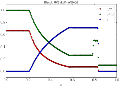
Appendix A Flat Spacetime 1D Tests

Table 4: Convergence results for the 1D simple wave test at $t=0.6$. The convergence rate $p$ is calculated dividing successive $L_{1}$ norm values.

Scheme	$n$	$L_{1}$	$p$	$L_{2}$	$p$
LLF-WENOZ	200	2.271e-03	-	6.431e-03	-
	400	5.974e-04	1.927	1.810e-03	1.829
	800	1.521e-04	1.974	4.657e-04	1.959
	1600	3.828e-05	1.990	1.174e-04	1.988
	3200	3.209e-06	1.997	1.698e-05	1.996
HO-WENOZ	200	5.988e-04	-	1.790e-03	-
	400	4.059e-05	3.883	1.512e-04	3.566
	800	1.677e-06	4.597	7.470e-06	4.339
	1600	5.623e-08	4.898	2.567e-07	4.863
	3200	6.089e-10	4.947	4.621e-09	5.002
LLF-MP5	200	7.579e-04	-	3.713e-03	-
	400	1.991e-04	1.928	1.043e-03	1.832
	800	5.081e-05	1.970	2.685e-04	1.957
	1600	1.281e-05	1.988	6.772e-05	1.987
	3200	3.209e-06	1.997	1.698e-05	1.996
HO-MP5	200	2.774e-04	-	1.466e-03	-
	400	1.365e-05	4.346	9.129e-05	4.005
	800	5.455e-07	4.645	4.334e-06	4.396
	1600	1.797e-08	4.924	1.487e-07	4.866
	3200	5.555e-10	5.016	4.576e-09	5.022

The implementation of the HO schemes in BAM has been tested against standard special relativistic hydrodynamics benchmarks. In particular, we present here the two 1D relativistic blast wave tests described in Marti and Müller (1999) and a 1D evolution of isentropic smooth waves Liang (1977); Anile (1990) (see also Colella et al. (2006); Zhang and MacFadyen (2005); Radice and Rezzolla (2012); Bugner et al. (2015) for similar tests). 1D benchmarks are important because exact solutions are available in these cases and, as already mentioned, the multi-D scheme is obtained by successive application of 1D procedures. In practice, only new 1D routines has been implemented for the HO algorithm.

The blast wave tests assess that the numerical scheme is nonoscillatory, handles solutions with shocks properly, and captures correctly all the elementary waves of the evolution of the Riemann problems. The evolution of simple waves is instead used to prove the scheme achieves high-order convergence for smooth flow solutions. For comparison, all the tests were also run with the second-order LLF scheme based on primitive reconstruction employing the same WENOZ or MP5 reconstruction as in the HO case. Let us stress that in the HO and LLF algorithms the same reconstruction is applied to different quantities: either projected fluxes or primitives variables.

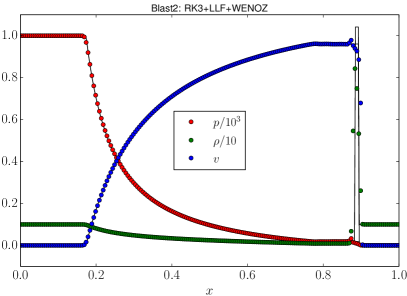
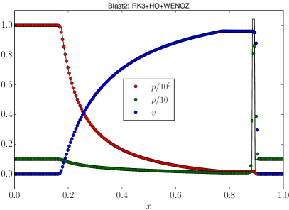
Initial data for the relativistic blast waves are set exactly as described in Marti and Müller (1999) (Problem 1 and 2), and a $\Gamma=5/3$ EOS is employed. The numerical solutions at $t=0.4$ are shown in Fig. 14. They are computed with $400$ grid points in the domain $[0,1]$ (resolution $h=0.0025$). The RK3 time integrator and CFL factor $0.25$ are used. The exact solution is also plotted as solid lines. As evident from the figures, the simulations reproduce all the features of the exact solution, and no relevant differences are found between the HO and the LLF scheme. (Note, however, a small difference in the resolution of the shock wave.)

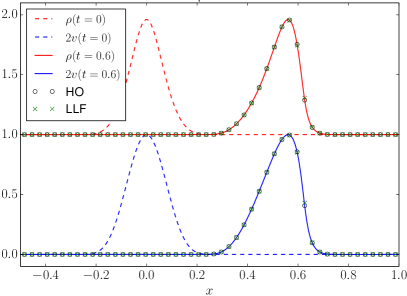
Relativistic simple waves are nonlinear elementary waves analogues of planar acoustic waves Liang (1977); Anile (1990). The exact solutions can be found implicitly by the method of characteristics. During the evolution, shock formation is expected in a finite time due to nonlinearities. Right-propagating simple wave initial data are set up by (i) choosing a reference state ($\rho=1$, $v=0$), (ii) prescribing a velocity perturbation, and (iii) computing the sound speed according to the value of the Riemann invariant (Eq. (II.15) of Liang (1977)). The other quantities follow from the EOS. The velocity profile is here set as,

$$v=a\ \Theta\left(|x|-X\right)\ \sin^{6}\left(\frac{\pi}{2}\left(\frac{x}{X}-1\right)\right)\ ,$$ (21)

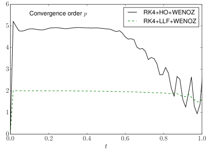
where $\Theta(x)$ is the Heaviside function, $a=0.5$ and $X=0.3$. Assuming a polytropic EOS with $\Gamma=5/3$ and $K=100$, the value of the sound speed in the reference state is $c_{s,0}\simeq 0.815$; the velocity and density initial profiles are shown in Fig. 15 (top). Note that the profile is smooth enough to guarantee that the WENO weights are close to optimal. Numerical solutions are computed on the domain $[-1.5,1.5]$, with the RK4 integrator and a CFL factor of $0.125$. During the evolution the initial profiles progressively steepen and finally a shock is formed  at around $t\simeq 0.63$. Figure 15 (top) shows the numerical solutions at $t=0.9$ for a resolution of $400$ points ($h=0.0075$). The exact solution is also plotted as solid lines. As evident, the simulations reproduce the correct physics. The formal convergence order of the numerical scheme can be checked at early times (before the shock forms). The bottom panel of Fig. 15 shows the self-convergence factor of a three-levels convergence test. In Tab. 4 we report the simulation errors as function in the $L_{1}$ and $L_{2}$ norms, at different resolutions and $t=0.6$. Both schemes converge to the exact solution at the expected rate for sufficiently high resolutions.

Appendix B Extrapolation in resolution alternative to the Richardson method

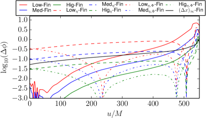
Ref. Hotokezaka et al. (2015) proposes a method for the resolution extrapolation that is alternative to the Richardson. In this appendix we apply that method to our SLy135135_006 data obtained with HOHyb-WENOZ scheme, and compare the results with those in Sec. VII.

Low resolution simulations are more affected by numerical dissipation than high resolution simulations. This results in earlier merger times for decreasing resolution. As a consequence, Ref. Hotokezaka et al. (2015) argues for the necessity to compensate for this effect by rescaling waveforms in time, $u\rightarrow\eta u$, and phase, $\phi\rightarrow\eta\phi$. The parameter $\eta$ is determined by minimizing

$$I_{2,1}=\min_{\eta^{\prime},\Phi}\int_{t_{i}}^{t_{f}}\text{d}u[A_{2,22}(\eta^{\prime}u)e^{i(\eta^{\prime}\phi_{2}(\eta^{\prime}u)+\Phi)}$$

$$-A_{1,22}(u)e^{i\phi_{1}(\eta)}]^{2},$$ (22)

where $A_{1,22},\phi_{{1,22}}$ refer to the amplitude and phase of the best resolved run and $A_{2,22},\phi_{{2,22}}$ to the other resolutions. We obtain the following values $\eta_{\rm L,F}=0.98651$, $\eta_{\rm M,F}=0.99584$, $\eta_{\rm H,F}=0.99867$. As in Hotokezaka et al. (2015) we estimate the convergence order $p$ from a three-level self-convergence test, for $\eta_{\rm M,F},\eta_{\rm H,F}$ we obtain $p=1.96$ and for $\eta_{\rm L,F},\eta_{\rm M,F}$ $p=2.34$. This allows us to scale the H-resolution data with a scaling parameter of $\eta_{\rm F,\infty}=0.99758$.

In Fig. 16 we compute the phase difference between the F-resolution and the (L,M,H)-simulations without shift, with $\eta$-shift, and with $\eta,\phi$-shift. We also include the phase difference between F-data and the waveform obtained with the extrapolation described above. We observe three main effects of the rescaling: (i) the phase difference during the beginning of the simulation increases; (ii) around $u_{\text{mrg}}$ the phase differences are smaller than for the nonshifted setup; (iii) we see zero crossing caused by the rescaling procedure.

Following Hotokezaka et al. (2015) the uncertainty is estimated by the relative uncertainty of the merger time multiplied by total phase of the simulation, i.e. $\Delta\phi=\phi(u_{\rm mrg})\;\Delta u_{\rm mrg}/u_{\rm mrg}$. For SLy135135_006, we have $\phi(u_{\rm mrg})\approx 40.8$ rad, $u_{\rm mrg}\approx 504M$. The difference $\Delta u$ is estimated either from the difference between the F-resolution and the extrapolated data as $\Delta u^{\rm mrg}=0.9M$, or based on the uncertainty of $p$ as extracted from the two different triplets to $\Delta u^{\rm mrg}=0.3M$, cf. Ref. Hotokezaka et al. (2015). Consequently the total uncertainty lies between $0.07$ and $0.025$ rad for two choices respectively. The optimistic uncertainty is a factor of $\sim 2$ smaller than the error assigned from the Richardson extrapolation. Because of the zero crossings, and the fact that the error budget strongly depends on the convergence order estimated solely from the merger time (at which the uncertainties are maximal), we prefer to use the simpler method outlined in Sec. VII.

Figure 16: Phase differences for Sly135135_006. Solid lines refer to the phase differences of the original data (L,M,H) to the highest resolved simulation (F). Dashed lines correspond to the phase difference between $\eta$ rescaled data and the original F-simulation. Dash-dotted lines are $\eta,\Phi$-rescaled data compared to H-resolution. The solid black line marks the difference of the extrapolated data to infinite resolution according to the text and F-resolution.

References

- Abbott et al. (2016) B. . Abbott et al. (Virgo, LIGO Scientific), Phys. Rev. Lett. 116, 061102 (2016), arXiv:1602.03837 [gr-qc] .
- Aasi et al. (2013) J. Aasi et al. (VIRGO, LIGO Scientific), (2013), arXiv:1304.0670 [gr-qc] .
- Bernuzzi et al. (2015) S. Bernuzzi, A. Nagar, T. Dietrich, and T. Damour, Phys.Rev.Lett. 114, 161103 (2015), arXiv:1412.4553 [gr-qc] .
- Baiotti et al. (2009) L. Baiotti, B. Giacomazzo, and L. Rezzolla, Class.Quant.Grav. 26, 114005 (2009), arXiv:0901.4955 [gr-qc] .
- Bernuzzi et al. (2012a) S. Bernuzzi, M. Thierfelder, and B. Brügmann, Phys.Rev. D85, 104030 (2012a), arXiv:1109.3611 [gr-qc] .
- Bernuzzi et al. (2012b) S. Bernuzzi, A. Nagar, M. Thierfelder, and B. Brügmann, Phys.Rev. D86, 044030 (2012b), arXiv:1205.3403 [gr-qc] .
- Reisswig et al. (2013) C. Reisswig, R. Haas, C. Ott, E. Abdikamalov, P. Mösta, et al., Phys.Rev. D87, 064023 (2013), arXiv:1212.1191 [astro-ph.HE] .
- Radice et al. (2014a) D. Radice, L. Rezzolla, and F. Galeazzi, Mon.Not.Roy.Astron.Soc. 437, L46 (2014a), arXiv:1306.6052 [gr-qc] .
- Hotokezaka et al. (2013) K. Hotokezaka, K. Kyutoku, and M. Shibata, Phys.Rev. D87, 044001 (2013), arXiv:1301.3555 [gr-qc] .
- Hotokezaka et al. (2015) K. Hotokezaka, K. Kyutoku, H. Okawa, and M. Shibata, Phys. Rev. D91, 064060 (2015), arXiv:1502.03457 [gr-qc] .
- Haas et al. (2016) R. Haas et al., (2016), arXiv:1604.00782 [gr-qc] .
- Harten et al. (1987) A. Harten, B. Engquist, S. Osher, and S. R. Chakrabarty, J. Comput. Phys. 71, 2311 (1987).
- Harten (1989) A. Harten, Journal of Computational Physics 83, 148 (1989).
- Shu and Osher (1989a) C. Shu and S. Osher, J. Comput. Phys. 77, 439 (1989a).
- Shu and Osher (1989b) C. Shu and S. Osher, J. Comput. Phys. 83, 32 (1989b).
- Liu et al. (1994) X.-D. Liu, S. Osher, and T. Chan, Journal of Computational Physics 115, 200 (1994).
- Jiang (1996) G. Jiang, J. Comp. Phys. 126, 202 (1996).
- Radice et al. (2014b) D. Radice, L. Rezzolla, and F. Galeazzi, Class.Quant.Grav. 31, 075012 (2014b), arXiv:1312.5004 [gr-qc] .
- Radice et al. (2015) D. Radice, L. Rezzolla, and F. Galeazzi, (2015), arXiv:1502.00551 [gr-qc] .
- Radice et al. (2016) D. Radice, S. Bernuzzi, and C. D. Ott, (2016), arXiv:1603.05726 [gr-qc] .
- Suresh (1997) A. Suresh, J. Comp. Phys. 136, 83 (1997).
- Hinderer et al. (2016) T. Hinderer et al., (2016), arXiv:1602.00599 [gr-qc] .
- Font (2007) J. A. Font, Living Rev. Rel. 11, 7 (2007).
- Douchin and Haensel (2001) F. Douchin and P. Haensel, Astron. Astrophys. 380, 151 (2001), astro-ph/0111092 .
- Read et al. (2009) J. S. Read, B. D. Lackey, B. J. Owen, and J. L. Friedman, Phys. Rev. D79, 124032 (2009), arXiv:0812.2163 [astro-ph] .
- Shibata et al. (2005) M. Shibata, K. Taniguchi, and K. Uryu, Phys. Rev. D71, 084021 (2005), arXiv:gr-qc/0503119 .
- Bauswein et al. (2010) A. Bauswein, H.-T. Janka, and R. Oechslin, Phys.Rev. D82, 084043 (2010), arXiv:1006.3315 [astro-ph.SR] .
- Thierfelder et al. (2011a) M. Thierfelder, S. Bernuzzi, and B. Brügmann, Phys.Rev. D84, 044012 (2011a), arXiv:1104.4751 [gr-qc] .
- Bernuzzi and Hilditch (2010) S. Bernuzzi and D. Hilditch, Phys. Rev. D81, 084003 (2010), arXiv:0912.2920 [gr-qc] .
- Hilditch et al. (2013) D. Hilditch, S. Bernuzzi, M. Thierfelder, Z. Cao, W. Tichy, et al., Phys. Rev. D88, 084057 (2013), arXiv:1212.2901 [gr-qc] .
- Nakamura et al. (1987) T. Nakamura, K. Oohara, and Y. Kojima, Prog. Theor. Phys. Suppl. 90, 1 (1987).
- Shibata and Nakamura (1995) M. Shibata and T. Nakamura, Phys. Rev. D52, 5428 (1995).
- Baumgarte and Shapiro (1999) T. W. Baumgarte and S. L. Shapiro, Phys. Rev. D59, 024007 (1999), arXiv:gr-qc/9810065 .
- Brügmann et al. (2008) B. Brügmann, J. A. Gonzalez, M. Hannam, S. Husa, U. Sperhake, et al., Phys.Rev. D77, 024027 (2008), arXiv:gr-qc/0610128 [gr-qc] .
- Thierfelder et al. (2011b) M. Thierfelder, S. Bernuzzi, D. Hilditch, B. Brügmann, and L. Rezzolla, Phys.Rev. D83, 064022 (2011b), arXiv:1012.3703 [gr-qc] .
- Dietrich et al. (2015) T. Dietrich, S. Bernuzzi, M. Ujevic, and B. Bruemann, Phys. Rev. D91, 124041 (2015), arXiv:1504.01266 [gr-qc] .
- Berger and Oliger (1984) M. J. Berger and J. Oliger, J.Comput.Phys. 53, 484 (1984).
- Xing and Shu (2012) Y. Xing and C.-W. Shu, Journal of Scientific Computing 54, 645 (2012).
- Mignone et al. (2010) A. Mignone, P. Tzeferacos, and G. Bodo, J.Comput.Phys. 229, 5896 (2010), arXiv:1001.2832 [astro-ph.HE] .
- Borges et al. (2008) R. Borges, M. Carmona, B. Costa, and W. S. Don, Journal of Computational Physics 227, 3191 (2008).
- Henrick et al. (2005) A. K. Henrick, T. D. Aslam, and J. M. Powers, Journal of Computational Physics 207, 542 (2005).
- Tchekhovskoy et al. (2007) A. Tchekhovskoy, J. C. McKinney, and R. Narayan, Mon. Not. Roy. Astron. Soc. 379, 469 (2007), arXiv:0704.2608 [astro-ph] .
- Bugner et al. (2015) M. Bugner, T. Dietrich, S. Bernuzzi, A. Weyhausen, and B. Bruegmann, (2015), arXiv:1508.07147 [gr-qc] .
- Gourgoulhon et al. (2001) E. Gourgoulhon, P. Grandclement, K. Taniguchi, J.-A. Marck, and S. Bonazzola, Phys.Rev. D63, 064029 (2001), arXiv:gr-qc/0007028 [gr-qc] .
- Weyhausen et al. (2012) A. Weyhausen, S. Bernuzzi, and D. Hilditch, Phys. Rev. D85, 024038 (2012), arXiv:1107.5539 [gr-qc] .
- Bernuzzi et al. (2016) S. Bernuzzi, D. Radice, C. D. Ott, L. F. Roberts, P. Moesta, and F. Galeazzi, Phys. Rev. D94, 024023 (2016), arXiv:1512.06397 [gr-qc] .
- Dietrich and Bernuzzi (2015) T. Dietrich and S. Bernuzzi, Phys.Rev. D91, 044039 (2015), arXiv:1412.5499 [gr-qc] .
- Reisswig and Pollney (2011) C. Reisswig and D. Pollney, Class.Quant.Grav. 28, 195015 (2011), arXiv:1006.1632 [gr-qc] .
- Bernuzzi et al. (2014) S. Bernuzzi, A. Nagar, S. Balmelli, T. Dietrich, and M. Ujevic, Phys.Rev.Lett. 112, 201101 (2014), arXiv:1402.6244 [gr-qc] .
- Boyle et al. (2007) M. Boyle et al., Phys. Rev. D76, 124038 (2007), arXiv:0710.0158 [gr-qc] .
- Lousto et al. (2010) C. O. Lousto, H. Nakano, Y. Zlochower, and M. Campanelli, Phys.Rev. D82, 104057 (2010), arXiv:1008.4360 [gr-qc] .
- Richardson (1911) L. F. Richardson, Philosophical Transactions of the Royal Society of London A: Mathematical, Physical and Engineering Sciences 210, 307 (1911).
- Hinder et al. (2013) I. Hinder, A. Buonanno, M. Boyle, Z. B. Etienne, J. Healy, et al., Class.Quant.Grav. 31, 025012 (2013), arXiv:1307.5307 [gr-qc] .
- Marti and Müller (1999) J. M. Marti and E. Müller, Living Rev. Rel. 2, 3 (1999), arXiv:astro-ph/9906333 .
- Liang (1977) E. P. T. Liang, Astrophys. J. 211, 361 (1977).
- Anile (1990) A. M. Anile, Relativistic Fluids and Magneto-fluids, by A. M. Anile, pp. 348. ISBN 0521304067. Cambridge, UK: Cambridge University Press, February 1990. (1990).
- Colella et al. (2006) P. Colella, D. T. Graves, B. J. Keen, and D. Modiano, Journal of Computational Physics 211, 347 (2006).
- Zhang and MacFadyen (2005) W.-Q. Zhang and A. I. MacFadyen, Astrophys.J.Suppl. (2005), arXiv:astro-ph/0505481 [astro-ph] .
- Radice and Rezzolla (2012) D. Radice and L. Rezzolla, (2012), arXiv:1206.6502 [astro-ph.IM] .