FlashR: R-Programmed Parallel and Scalable Machine Learning using SSDs
Abstract
R is one of the most popular programming languages for statistics and machine learning, but the R framework is relatively slow and unable to scale to large datasets. The general approach for speeding up an implementation in R is to implement the algorithms in C or FORTRAN and provide an R wrapper. FlashR takes a different approach: it executes R code in parallel and scales the code beyond memory capacity by utilizing solid-state drives (SSDs) automatically. It provides a small number of generalized operations (GenOps) upon which we reimplement a large number of matrix functions in the R base package. As such, FlashR parallelizes and scales existing R code with little/no modification. To reduce data movement between CPU and SSDs, FlashR evaluates matrix operations lazily, fuses operations at runtime, and uses cache-aware, two-level matrix partitioning. We evaluate FlashR on a variety of machine learning and statistics algorithms on inputs of up to four billion data points. FlashR out-of-core tracks closely the performance of FlashR in-memory. The R code for machine learning algorithms executed in FlashR outperforms the in-memory execution of H2O and Spark MLlib by a factor of and outperforms Revolution R Open by more than an order of magnitude.
1 Introduction
The explosion of data volume and the increasing complexity of data analysis generate a growing demand for scalable statistical analysis and machine learning tools that are simple and efficient. Simple tools need to be programmable, interactive, and extensible, allowing scientists to encode and deploy complex algorithms. Successful examples include R, SciPy, and Matlab. Efficiency dictates that tools should leverage modern computer architectures, including scalable parallelism, high-speed networking, and fast I/O from memory and solid-state storage. The current approach for utilizing the full capacity of modern parallel systems often uses a low-level programming language such as C and parallelizes computation with MPI or OpenMP. This approach is time-consuming and error-prone, and requires machine learning researchers to have expert knowledge in the parallel programming models.
While conventional wisdom addresses large-scale data analysis and machine learning with clusters [6, 33, 7, 1, 32, 14], recent works [35, 37, 16, 17] demonstrate a single-machine solution can deal with large-scale data analysis efficiently in a multicore machine. The advance of solid-state drives (SSDs) allows us to tackle data analysis in a single machine efficiently at a larger scale with a cheaper price. Previous SSD-based graph analysis frameworks [35, 37, 13] have demonstrated the comparable efficiency to state-of-the-art in-memory graph analysis, while scaling to arbitrarily large datasets. This work extends these findings to matrix operations using SSDs for machine learning and data analysis.
To provide a simple programming environment for efficient and scalable machine learning, we present FlashR, an interactive R-based programming framework that executes R code in parallel and out-of-core automatically. FlashR stores large vectors and matrices on SSDs and overrides many R functions in the R base package to perform computation on these external-memory vectors and matrices. As such, FlashR executes existing R code with little/no modification. FlashR focuses on optimizations in a single machine (with multiple CPUs and many cores) and scales matrix operations beyond memory capacity by utilizing solid-state drives (SSDs). Our evaluation shows that we can solve billion row, Internet-scale problems on a single thick node, which can prevent the complexity, expense, and power consumption of distributed systems when they are not strictly necessary [17].
To utilize the full capacity of a large parallel machine, we overcome many technical challenges to move data from SSDs to CPU efficiently for matrix computations, notably the large performance disparities between CPU and memory and between memory and SSDs. The “memory gap” [31] continues to grow, with the difference between CPU and DRAM performance increasing exponentially. There are also performance differences between local and remote memory in a non-uniform memory architecture (NUMA), which are prevalent in modern multiprocessor machines. RAM outperforms SSDs by an order of magnitude for both latency and throughput.
FlashR evaluates expressions lazily and fuses operations aggressively in a single parallel execution job to minimize data movement. FlashR builds a directed acyclic graph (DAG) to represent a sequence of matrix operations and grows a DAG as much as possible to increase the ratio of computation to I/O. When evaluating the computation in a DAG, FlashR performs two levels of matrix partitioning to reduce data movement in the memory hierarchy. FlashR by default materializes only the output matrices (leaf nodes) of a DAG and keeps materialized results in memory in order to minimize data written to SSDs. FlashR streams data from SSDs to maximize I/O throughput for most computation tasks.
We implement multiple machine learning algorithms, including principal component analysis, logistic regression and k-means, in FlashR. On a large parallel machine with 48 CPU cores and fast SSDs, the out-of-core execution of these R implementations achieves performance comparable to their in-memory execution, while significantly outperforming the same algorithms in H2O [8] and Spark MLlib [33]. FlashR effortlessly scales to datasets with billions of data points and its out-of-core execution uses a negligible amount of memory compared with the dataset size. In addition, FlashR executes the R functions in the R MASS [15] package with little modification and outperforms the execution of the same functions in Revolution R Open [23] by more than an order of magnitude.
We believe that FlashR significantly lowers the requirements for writing parallel and scalable implementations of machine learning algorithms; it also offers new design possibilities for data analysis clusters, replacing memory with larger and cheaper SSDs and processing bigger problems on fewer nodes. FlashR is released as an open-source project at http://flashx.io/.
2 Related Work
Basic Linear Algebra Subprograms (BLAS) defines a small set of vector and matrix operations. There exist a few highly-optimized BLAS implementations, such as MKL [19] and ATLAS [30]. Distributed libraries [9, 2, 21] build on BLAS and distribute computation with MPI. BLAS provides a limited set of matrix operations and requires users to manually parallelize the remaining matrix operations.
Recent works on out-of-core linear algebra [27, 22] redesign algorithms to achieve efficient I/O access and reduce I/O complexity. These works are orthogonal to our work and can be adopted. Optimizing I/O alone is insufficient. To achieve performance comparable to state-of-the-art in-memory implementations, it is essential to move data efficiently both from SSDs to memory and from memory to CPU caches.
MapReduce [6] has been used for parallelizing machine learning algorithms [4]. Even though MapReduce simplifies parallel programming, it still requires low-level programming. As such, frameworks are built on top of MapReduce to reduce programming complexity. For example, SystemML [7] develops an R-like script language for machine learning. MapReduce is inefficient for matrix operations because its I/O streaming primitives do not match matrix data access patterns.
The Spark [33] is a distributed, in-memory framework that provides more primitives for efficient computation and provides a distributed machine learning library (MLlib, [18]). Spark is the most efficient distributed engine.
Distributed machine learning frameworks have been developed to train machine learning models on large datasets. For example, GraphLab [14] formulates machine learning algorithms as graph computation; Petuum [32] is designed for machine learning algorithms with certain properties such as error tolerance; TensorFlow [1] trains machine learning models, especially deep neural networks, with optimization algorithms such as stochastic gradient descent.
Efforts to parallelize array programming include Revolution R [23] and Matlab’s parallel computing toolbox, which offer multicore parallelism and explicit distributed parallelism using MPI and MapReduce. Other works focus on implicit parallelization. Presto [28] extends R to sparse matrix operations in distributed memory for graph analysis. Ching et. al [3] parallelize APL code by compiling it to C. Accelerator [26] compiles data-parallel operations on the fly to execute programs on a GPU.
OptiML [24] is a domain-specific language for developing machine learning in a heterogeneous computation environment such as multi-core processors and GPU. It designs a new programming language and relies on a compiler to generate code for the heterogenous environment.
3 Design
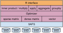
FlashR is a matrix-oriented programming framework for machine learning and statistics. It scales matrix operations beyond memory capacity by utilizing fast I/O devices, such as solid-state drives (SSDs), in a non-uniform memory architecture (NUMA) machine. Figure 1 shows the architecture of FlashR. FlashR has only a few classes of generalized operations (GenOps) to simplify the implementation and the GenOps improve expressiveness of the framework. The optimizer aggressively merges operations to reduce data movement in the memory hierarchy. It stores matrices on SSDs through SAFS [34], a user-space filesystem for SSD arrays, to fully utilize high I/O throughput of SSDs.
3.1 Programming interface
FlashR provides a matrix-oriented functional programming interface built on Generalized Operations (GenOps). GenOps (Table 1) take matrices and some functions as input and output new matrices that represent computation results. The input function defines computation on individual elements in input matrices. GenOps provide a flexible and concise programming interface and, thus, we focus on optimizing the small set of matrix operations. All of the GenOps are lazily evaluated to gain efficiency (Section 3.4).
| GenOp | Description |
|---|---|
| , over all , | |
| , over all | |
| , over all | |
| , | |
| where , over all | |
| , | |
| where , over all | |
| , | |
| where , over all | |
| , | |
| , over all |
GenOps are classified into four categories that describe different data access patterns.
Element-wise operations: sapply is an element-wise unary operation; mapply is an element-wise binary operation; mapply.row and mapply.col perform element-wise binary operations on the input vector with every row or column of the input matrix and output a matrix of the same shape as the input matrix.
Aggregation: agg computes aggregation over all elements in a matrix and outputs a scalar value; agg.row computes over all elements in every row and outputs a vector; agg.col computes over all elements in every column and outputs a vector.
Groupby: groupby splits the elements of a matrix into groups, applies agg to each group and outputs a vector; groupby.row splits rows into groups and applies agg.col to each group; groupby.col splits columns into groups and applies agg.row to each group. Both agg.row and agg.col output a matrix.
Inner product is a generalized matrix multiplication that replaces multiplication and addition with two functions.
We reimplement a large number of matrix functions in the R base package with the GenOps to provide users a familiar programming interface. By overriding existing R matrix functions, FlashR scales and parallelizes existing R code with little/no modification. Table 2 shows a small subset of R matrix operations and their implementations with GenOps.
| Function | Implementation with GenOps |
|---|---|
| for integers; | |
| use BLAS for floating-point values; | |
| use SpMM [36] for sparse matrices. |
In addition to computation operations, FlashR provides functions for matrix construction and data access in a FlashR matrix (Table 3). This includes creating vectors and matrices, loading matrices from an external source, interacting with the R framework, reshaping a matrix, accessing rows and columns of a matrix and so on. FlashR avoids unnecessary data movement in these functions. For example, transpose of a matrix does not physically move elements in the matrix and instead, it causes FlashR to access data in the matrix differently in the subsequent matrix operations.
| Function | Description |
|---|---|
| Create a vector of a repeated value | |
| Create a vector of sequence numbers | |
| Create a uniformly random matrix | |
| Create a matrix under a normal distribution | |
| Load a dense matrix to FlashR | |
| Load a sparse matrix to FlashR | |
| Convert a FlashR matrix to an R matrix | |
| Convert an R matrix to a FlashR matrix | |
| Matrix transpose | |
| Concatenate matrices by rows | |
| Concatenate matrices by columns | |
| Get rows or columns from a matrix |
3.2 Dense matrices
FlashR optimizes for dense matrices that are rectangular—with a longer and shorter dimension—because of their frequent occurrence in machine learning and statistics. Dense matrices can be stored physically in memory or on SSDs or represented virtually by a sequence of computations.
3.2.1 Tall-and-skinny (TAS) matrices
A data matrix may contain a large number of samples with a few features (tall-and-skinny), or a large number of features with a few samples (wide-and-short). We use similar strategies to optimize wide-and-short matrices. FlashR supports both row-major and column-major layouts (Figure 2(a) and (b)), which allows FlashR to transpose matrices without a copy. We store vectors as a one-column TAS matrix.
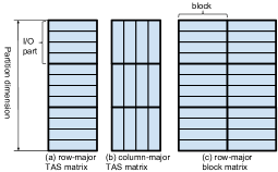
A TAS matrix is partitioned physically into I/O-partitions (Figure 2). We refer to the dimension that is partitioned as partition dimension. All elements in an I/O-partition are stored contiguously regardless of the data layout in the matrix. All I/O-partitions have the same number of rows regardless of the number of columns in a TAS matrix. The number of rows in an I/O-partition is always . This produces column-major TAS matrices whose data are well aligned in memory to help CPU vectorization.
When a TAS matrix is stored in memory, FlashR stores its I/O partitions in fixed-size memory chunks (e.g., 64MB) across NUMA nodes. I/O partitions from different matrices may have different sizes. By storing I/O partitions in fixed-size memory chunks shared among all in-memory matrices, FlashR can easily recycle memory chunks to reduce memory allocation overhead.
When a TAS matrix is stored on SSDs, it is stored as a SAFS file [34]. For such a matrix, an I/O partition is accessed in a single I/O request. We rely on SAFS to map the data of a matrix evenly across SSDs. SAFS allows applications to specify the data mapping strategies. By default, FlashR uses a hash function to map data to SSDs to fully utilize the bandwidth of all SSDs even if we access only a subset of columns from a TAS matrix.
3.2.2 Block matrices
FlashR stores a tall matrix as a block matrix (Figure 2(c)) comprised of TAS blocks with columns each, except the last block. Each block is stored as a separate TAS matrix. We decompose a matrix operation on a block matrix into operations on individual TAS matrices to take advantage of the optimizations on TAS matrices and reduce data movement. Coupled with the I/O partitioning on TAS matrices, this strategy enables 2D-partitioning on a dense matrix and each partition fits in main memory.
3.2.3 Virtual matrices
To support lazy evaluation, FlashR uses virtual matrices that materialize data on the fly during computation and transfer output as input to the matrix operation. The data of a matrix are not stored physically. All GenOps output virtual matrices. A GenOp on a block matrix may output a block virtual matrix. Virtual matrices are assembled to construct a directed acyclic graph (DAG) that represents a sequence of matrix computations (Section 3.4.1). Virtual matrices are essential to reduce data movement in the memory hierarchy and memory allocation overhead to accelerate computation.
3.2.4 Sink matrices
The leaf nodes in a DAG are sink matrices. These are produced by aggregation, groupby, and inner product GenOps for which the output matrices have a different partition dimension size than the input matrices. Sink matrices tend to be small and we store their results in memory. The maximum size of a sink matrix from an aggregation is for elements in the input matrix and for groupby for groups, where is usually a small number. For most of machine learning and data analysis tasks, the output of inner product of a wide matrix with a tall matrix is small because the long dimension of these matrices is much larger than the short dimension.
3.3 Sparse matrices
FlashR supports sparse matrices and optimizes sparse matrices of different shapes differently. For large sparse matrices that arise from graphs (e.g., social networks and Web graphs), which have a large number of rows and columns, FlashR integrates with our prior work [36] that stores sparse matrices in a compact format on SSDs and performs sparse matrix multiplication in semi-external memory, i.e., we keep the sparse matrix on SSDs and the dense matrix or part of the dense matrix in memory. Because many graph algorithms can be formulated with sparse matrix multiplication [10], we can express these algorithms in FlashR. In contrast, for sparse matrices with many rows and few columns or with many columns and few rows, FlashR stores the sparse matrices with the coordinate format (COO). These sparse matrices can be used in sparse random projection [11] or to store categorial values for computation. FlashR keeps these sparse matrices in memory.
3.4 Reducing data movement
It is essential to reduce data movement within the memory hierarchy to achieve efficiency when evaluating a sequence of matrix operations. FlashR lazily evaluates most matrix operations, especially the ones that do not contain heavy computation, and constructs one or more directed-acyclic graphs (DAGs) connecting GenOps and matrices. Figure 3 (a) shows a DAG for an iteration of k-means. It performs all computation in a DAG together, which creates opportunities for fusing matrix operations to reduce data movement in the memory hierarchy. This data-driven, lazy evaluation allows out-of-core problems to approach in-memory speed.
3.4.1 Directed-acyclic graphs (DAGs)
A DAG comprises a set of matrix nodes (rectangles) and computation nodes (ellipses) (Figure 3 (b)). The majority of matrix nodes are virtual matrices (dashed line rectangles). For k-means, only the input matrix X has materialized data. A computation node references a GenOp and input matrices and may contain some immutable computation state, such as scalar variables and small matrices.
FlashR grows each DAG as large as possible, by allowing virtual matrices of different shapes in a DAG, to increase the ratio of computation to I/O (Figure 3). All virtual matrices in internal matrix nodes have the same partition dimension size to simplify evaluation and data flow. Sink matrices are edge nodes in the DAG because they have different partition dimension sizes from the internal matrices. Any computation that uses these sink matrices cannot be connected to the same DAG.
3.4.2 DAG materialization
FlashR allows both explicit and implicit DAG materialization to simplify programming while providing the opportunities to tune the code for better speed. For explicit materialization, a user can invoke fm.materialize to materialize a virtual matrix. Access to elements of a sink matrix triggers materialization implicitly. Materialization on a virtual matrix triggers materialization on the DAG where the virtual matrix connects.
By default, FlashR saves the computation results of all sink matrices of the DAG in memory and discard the data of non-sink matrices on the fly. Because sink matrices tend to be small, this materialization rule leads to small memory consumption. In exceptional cases, especially for iterative algorithms, it is helpful to save some non-sink matrices to avoid redundant computation and I/O across iterations. We allow users to set a flag on any virtual matrix to materialize and cache data in memory or on SSDs during computation, similar to caching a resilient distributed dataset (RDD) in Spark [33].
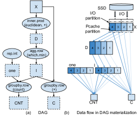
FlashR partitions matrices in a DAG and materializes partitions separately. This is possible because all matrices, except sink matrices, share the same partition dimension. A partition of a virtual matrix requires data only from partitions of the parent matrices. All DAG operations in a partition are processed by the same thread so that all data required by the computations are stored and accessed in the memory close to the processor to increase the memory bandwidth in a NUMA machine. When materializing a sink matrix, each thread computes partial aggregation results on the partitions assigned to the thread. Then, FlashR merges per-thread partial results to construct the output.
FlashR uses two-level partitioning on dense matrices to reduce data movement between SSDs and CPU (Figure 3 (b)). It reads data on SSDs in I/O partitions and assigns these partitions to a thread as a parallel task. It further splits I/O-partitions into processor cache (Pcache) partitions at run time. Each thread materializes one Pcache-partition at a time. Matrix operations run on TAS matrices or block matrices are divided into TAS matrices so that a Pcache-partition fits in the CPU L1/L2 cache.
FlashR makes an effort to increase hits in the CPU cache, which significantly reduces data movement between CPU and memory. When materializing output to a virtual matrix, the thread passes the output as input to the subsequent GenOp, instead of materializing the next Pcache-partition. This ensures that a Pcache-partition resides in the CPU cache when the next GenOp consumes it. In each thread, all intermediate matrices have only one Pcache-partition materialized at any time to reduce CPU cache pollution.
3.5 Parallel execution and I/O access
FlashR dispatches computation to threads so that they issue large reads and writes to SSDs, while still achieving good load balancing. FlashR uses a global task scheduler to assign I/O-partitions to threads dynamically. Initially, the scheduler assigns multiple contiguous I/O-partitions to a thread. The thread reads these in a single large I/O. The number of contiguous I/O-partitions assigned to a thread is determined by the block size of SAFS. As the computation nears an end, the scheduler dispatches single I/O-partitions. The scheduler dispatches I/O-partitions sequentially to maximize contiguity in memory and on SSD. When the DAG stores the materialized result of a non-sink matrix, contiguity makes it easier for the file system to merge writes from multiple threads, which helps to sustain write throughput and reduces write amplification [25].
4 Machine learning algorithms
To illustrate the programming interface of FlashR, we showcase some classic algorithms written in FlashR. Some of the algorithms can be implemented with R base functions and can run in the existing R framework without any modification.
K-means is a commonly used clustering algorithm that partitions data points into clusters so that each cluster has the minimal mean distance between the data points and the cluster center. We use this algorithm to illustrate programming with GenOps (Figure 4). It first uses inner.prod to compute the Euclidean distance between every data point and every cluster center and outputs a matrix with each row representing the distances to centers. It uses agg.row to find the closest cluster for each data point. The output matrix assigns data points to clusters. It then uses groupby.row to count the number of data points in each cluster and compute the mean of each cluster.
Logistic regression is a commonly used classification algorithm. We implement this algorithm solely with the R base functions overriden by FlashR. Figure 5 implements logistic regression for problems with binary-class labels. It uses steepest gradient descent with line search to minimize the cost function. This example does not have a regularization term in the cost function.
PageRank is a well-known algorithm for graph analysis. The matrix formulation (Figure 6) operates on the adjacency matrix of a graph. It uses a power method and performs a sequence of sparse matrix multiplications until the algorithm converges.
5 Experimental evaluation
We evaluate the efficiency of FlashR on statistics and machine learning algorithms both in memory and on SSDs. We compare the R implementations of these algorithms with the ones in two optimized parallel machine learning libraries H2O [8] and Spark MLlib [18]. We further use FlashR to accelerate existing R functions in the MASS package and compare with Revolution R Open [23].
We conduct experiments on a NUMA machine with four Intel Xeon E7-4860 2.6 GHz processors and 1TB of DDR3-1600 memory. Each processor has 12 cores. The machine is equipped with 24 OCZ Intrepid 3000 SSDs, which together are capable of 12 GB/s for read and 10 GB/s for write. The machine runs Ubuntu 14.04 and uses ATLAS 3.10.1 as the default BLAS library.
5.1 Benchmark algorithms
We benchmark FlashR with some commonly used algorithms. Like the algorithms shown in Section 4, we implement these algorithms completely with the R code and rely on FlashR to execute them in parallel and out of core.
Correlation computes pair-wise Pearson’s correlation [20] and is commonly used in statistics.
Principal Component Analysis (PCA) computes uncorrelated variables from a large dataset. PCA is commonly used for dimension reduction in many data analysis tasks. We compute PCA by computing eigenvalues on the Gramian matrix of the input matrix .
Naive Bayes is a classifier that applies Bayes’ theorem with the “naive” assumption of independence between every pair of features. Our implementation assumes data follows the normal distribution.
Logistic regression is a linear regression model with categorical dependent variables. We use the Newton-CG algorithm to optimize logistic regression. It converges when , where is the logarithmic loss at iteration .
K-means is an iterative clustering algorithm that partitions data points to clusters. Its R implementation is illustrated in Figure 4. In the experiments, we run k-means to split a dataset into 10 clusters by default. It converges when no data points move.
Multivariate Normal Distribution (mvrnorm) generates samples from the specified multivariate normal distribution. We use the implementation in the MASS package.
Linear discriminant analysis (LDA) is a linear classifier that assumes the normal distribution with a different mean for each class but sharing the same covariance matrix among classes. Our LDA is adapted from the one in the R MASS package only with some trivial modifications.
PageRank is a well-known algorithm for graph analysis. We run the R implementation in Figure 6 in the experiment. PageRank converges when , where is the PageRank value of vertex at iteration and is the number of vertices in the graph.
| Algorithm | Computation | I/O |
|---|---|---|
| Correlation | ||
| PCA | ||
| Naive Bayes | ||
| Logistic regression | ||
| K-means | ||
| mvrnorm | ||
| LDA | ||
| PageRank |
These algorithms have various ratios of computation complexity and I/O complexity (Table 4) to thoroughly evaluate performance of FlashR on SSDs. Logistic regression, K-means and PageRank run iteratively and, thus, we show their computation and I/O complexity in a single iteration.
We benchmark FlashR with two real-world datasets with billions of data points (Table 5). The Criteo dataset has over four billion data points with binary labels (click vs. no-click), used for advertisement click prediction [5]. PageGraph is the adjacency matrix of a graph whose vertices represent Web pages and edges represents hyperlinks between Web pages [29]. PageGraph-32ev are 32 singular vectors that we computed on the largest connected component of Pagegraph with the tools we built previously [35, 36]. To compare FlashR with other frameworks, we take part of the Criteo and PageGraph-32ev datasets to create smaller datasets. PageGraph-32ev-sub is the first 336 million data points of the PageGraph-32ev dataset. Criteo-sub contains the data points collected on the first two days, which is about one tenth of the whole dataset.
5.2 Comparative performance
We evaluate FlashR against H2O [8] and Spark MLlib [18] as well as Revolution R Open [23] in a large parallel machine with 48 CPU cores and in the Amazon cloud. When running in the 48 CPU core machine, all frameworks use 48 threads and H2O and MLlib have a large heap size (500GB) to ensure that all data are cached in memory. When running in the cloud, we run FlashR in a single i2.8xlarge instance (16 CPU cores, 244GB RAM and 6.4TB SSD storage) and MLlib in a cluster of four EC2 c4.8xlarge instances (72 CPU cores, 240GB RAM and 10Gbps network). We also use FlashR to parallelize functions (mvrnorm and LDA) in the R MASS package and compare their speed with Revolution R Open. We use Spark v2.0.1, H2O v3.10.2 and Revolution R Open v3.3.2.
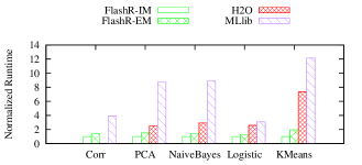
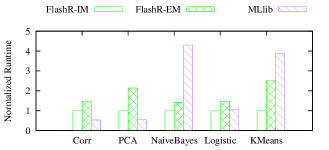
FlashR outperforms H2O and Spark MLlib significantly on all algorithms (Figure 7(a)) in the large parallel machine with 48 CPU cores. FlashR running in memory achieves 3 to 10 times performance gain when compared with MLlib, and 2.5 to 7 times performance gain when compared with H2O. When running on SSDs, FlashR achieves at least half the speed of running in memory. Even though logistic regression in FlashR uses Newton-CG, a much more computation intensive optimization algorithm than LBFGS [12] used by H2O and MLlib (Newton-CG takes 10 iterations and LBFGS takes 14 iterations to converge to similar loss on the dataset), FlashR still runs almost times as fast as H2O and MLlib. All implementations rely on BLAS for matrix multiplication. H2O and MLlib have to implement non-BLAS operations with Java and Scala, respectively, and MLlib materializes operations such as aggregation separately. In contrast, FlashR fuses matrix operations and performs two-level partitioning to minimize data movement in the memory hierarchy and keeps data in local memory to achieve high memory bandwidth.
We further evaluate the speed of FlashR on Amazon EC2 cloud and compare it with Spark MLlib on an EC2 cluster (Figure 7(b)). Spark MLlib needs at least 4 c4.8xlarge instances to process the datasets (PageGraph-32ev-sub and Criteo-sub). Even though Spark MLlib has 4.5 as much computation power as FlashR, FlashR at least matches the speed of Spark MLlib and even outperforms it.

FlashR running both in memory and on SSDs outperforms Revolution R Open by more than an order of magnitude even on a small dataset ( and ) (Figure 8). Revolution R Open uses Intel MKL to parallelize matrix multiplication. As such, we only compare the two frameworks with computations that use matrix multiplication heavily. Both FlashR and Revolution R Open run the mvrnorm and LDA implementations from the MASS package. For simple matrix operations such as crossprod, FlashR slightly outperforms Revolution R Open. For more complex computations, the speed gap between FlashR and Revolution R increases. Even though matrix multiplication is the most computation-intensive operation in an algorithm, it is insufficient to only parallelize matrix multiplication to achieve high efficiency.
5.3 Scalability
We show the scalability of FlashR on the billion-scale datasets in Table 5. In these experiments, we run the iterative algorithms on the datasets until they converge (see their convergence condition in Section 5.1).
| Runtime (s) | Memory (GB) | |
|---|---|---|
| Correlation | ||
| PCA | ||
| NaiveBayes | ||
| LDA | ||
| Logistic regression | ||
| k-means | ||
| PageRank |
Even though we process the billion-scale datasets in a single machine, none of the algorithms are prohibitively expensive. Simple algorithms, such as Naive Bayes and PCA, require one or two passes over the datasets and take only one or two minutes to complete. Logistic regression and k-means take about iterations to converge. Because the PageRank implementation uses the power method, it takes iterations to converge. Nevertheless, all of the iterative algorithms take about one hour or less.
FlashR scales to datasets with billions of data points easily when running out of core. Most of the algorithms have negligible memory consumption. PageRank consumes more memory because the sparse matrix multiplication in PageRank keeps vectors in memory for semi-external memory computation. The scalability of FlashR is mainly bound by the capacity of SSDs. The functional programming interface generates a new matrix in each matrix operation, which potentially leads to high memory consumption. Thanks to lazy evaluation and virtual matrices, FlashR only needs to materialize the small matrices to effectively reduce memory consumption.
5.4 Computation complexity versus I/O complexity
We further compare the speed of FlashR in memory and in external memory for algorithms with different computation and I/O complexities. We pick three algorithms from Table 4: (i) Naive Bayes, whose computation and I/O complexity are the same, (ii) correlation, whose computation complexity grows quadratically with while its I/O complexity grows linearly with , (iii) k-means, whose computation complexity grows linearly with while its I/O complexity is independent to . We run the first two algorithms on datasets with and varying from 8 to 512. We run k-means on a dataset with and and vary the number of clusters from 2 to 64.
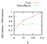
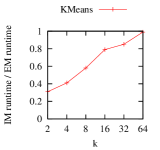
As the number of features or clusters increases, the performance gap between in-memory and external-memory execution narrows and the external-memory performance approaches in-memory performance for correlation and k-means but not Naive Bayes (Figure 9). This observation conforms with the computation and I/O complexity of the algorithms in Table 4. For correlation and k-means, the number of clusters or features causes computation to grow more quickly than the I/O, driving performance toward a computation bound. The computation bound can be realized on few features or clusters for an I/O throughput of 10GB/s. Because most of the machine learning algorithms in Table 4 have computation complexities that grow quadratically with , we expect FlashR on SSDs to achieve the same speed as in memory on datasets with a higher dimension size.
6 Conclusions
We present FlashR, a matrix-oriented programming framework that executes R-programmed machine learning algorithms in parallel and out-of-core automatically. FlashR scales to large datasets by utilizing commodity SSDs.
Although R is considered to be slow and unable to scale to large datasets, we demonstrate that with sufficient system-level optimizations, FlashR powers the R programming interface to achieve high performance and scalability for developing many machine learning algorithms. R implementations executed in FlashR outperform H2O and Spark MLlib on all algorithms by a large factor, using the same shared memory hardware. FlashR scales to datasets with billions of data points easily with negligible amounts of memory and completes all algorithms within a reasonable amount of time.
Even though SSDs are an order of magnitude slower than DRAM, the external-memory execution of many algorithms in FlashR achieve performance approaching their in-memory execution. We demonstrate that an I/O throughput of 10 GB/s saturates the CPU for many algorithms, even in a large parallel NUMA machine.
FlashR simplifies the programming effort of writing parallel and out-of-core implementations for large-scale machine learning. With FlashR, machine learning researchers can prototype algorithms in a familiar programming environment, while still getting efficient and scalable implementations. We believe FlashR provides new opportunities for developing large-scale machine learning algorithms.
References
- [1] Abadi, M., Barham, P., Chen, J., Chen, Z., Davis, A., Dean, J., Devin, M., Ghemawat, S., Irving, G., Isard, M., Kudlur, M., Levenberg, J., Monga, R., Moore, S., Murray, D. G., Steiner, B., Tucker, P., Vasudevan, V., Warden, P., Wicke, M., Yu, Y., and Zheng, X. Tensorflow: A system for large-scale machine learning. In 12th USENIX Symposium on Operating Systems Design and Implementation (OSDI 16) (2016).
- [2] Balay, S., Abhyankar, S., Adams, M. F., Brown, J., Brune, P., Buschelman, K., Dalcin, L., Eijkhout, V., Gropp, W. D., Kaushik, D., Knepley, M. G., McInnes, L. C., Rupp, K., Smith, B. F., Zampini, S., and Zhang, H. PETSc Web page. http://www.mcs.anl.gov/petsc, 2015.
- [3] Ching, W.-M., and Zheng, D. Automatic parallelization of array-oriented programs for a multi-core machine. International Journal of Parallel Programming 40, 5 (2012), 514–531.
- [4] Chu, C.-T., Kim, S. K., Lin, Y.-A., Yu, Y., Bradski, G., Ng, A. Y., and Olukotun, K. Map-reduce for machine learning on multicore. In Proceedings of the 19th International Conference on Neural Information Processing Systems (2006).
- [5] Criteo’s 1tb click prediction dataset. https://blogs.technet.microsoft.com/machinelearning/2015/04/01/now-available-on-azure-ml-criteos-1tb-click-prediction-dataset/, Accessed 2/11/2017.
- [6] Dean, J., and Ghemawat, S. MapReduce: Simplified data processing on large clusters. In Proceedings of the 6th Conference on Symposium on Opearting Systems Design & Implementation - Volume 6 (Berkeley, CA, USA, 2004), OSDI’04, USENIX Association.
- [7] Ghoting, A., Krishnamurthy, R., Pednault, E., Reinwald, B., Sindhwani, V., Tatikonda, S., Tian, Y., and Vaithyanathan, S. SystemML: Declarative machine learning on mapreduce. In Proceedings of the 2011 IEEE 27th International Conference on Data Engineering (Washington, DC, USA, 2011), IEEE Computer Society.
- [8] H2o machine learning library. http://www.h2o.ai/, Accessed 2/7/2017.
- [9] Heroux, M. A., Bartlett, R. A., Howle, V. E., Hoekstra, R. J., Hu, J. J., Kolda, T. G., Lehoucq, R. B., Long, K. R., Pawlowski, R. P., Phipps, E. T., Salinger, A. G., Thornquist, H. K., Tuminaro, R. S., Willenbring, J. M., Williams, A., and Stanley, K. S. An overview of the Trilinos project. ACM Trans. Math. Softw. (2005).
- [10] Kepner, J., and Gilbert, J. Graph Algorithms in the Language of Linear Algebra. Society for Industrial & Applied Mathematics, 2011.
- [11] Li, P., Hastie, T. J., and Church, K. W. Very sparse random projections. In Proceedings of the 12th ACM SIGKDD International Conference on Knowledge Discovery and Data Mining (2006).
- [12] Liu, D. C., and Nocedal, J. On the limited memory bfgs method for large scale optimization. Mathematical Programming: Series A and B (1989).
- [13] Liu, H., and Huang, H. H. Graphene: Fine-grained io management for graph computing. In 15th USENIX Conference on File and Storage Technologies (FAST 17) (Santa Clara, CA, 2017).
- [14] Low, Y., Bickson, D., Gonzalez, J., Guestrin, C., Kyrola, A., and Hellerstein, J. M. Distributed graphlab: A framework for machine learning and data mining in the cloud. Proc. VLDB Endow. 5, 8 (2012).
- [15] Package mass. https://cran.r-project.org/web/packages/MASS/index.html, Accessed 2/12/2017.
- [16] Matveev, A., Meirovitch, Y., Saribekyan, H., Jakubiuk, W., Kaler, T., Odor, G., Budden, D., Zlateski, A., and Shavit, N. A multicore path to connectomics-on-demand. In Proceedings of the 22Nd ACM SIGPLAN Symposium on Principles and Practice of Parallel Programming (2017).
- [17] McSherry, F., Isard, M., and Murray, D. G. Scalability! but at what cost? In 15th Workshop on Hot Topics in Operating Systems (HotOS XV) (2015).
- [18] Meng, X., Bradley, J., Yavuz, B., Sparks, E., Venkataraman, S., Liu, D., Freeman, J., Tsai, D., Amde, M., Owen, S., Xin, D., Xin, R., Franklin, M. J., Zadeh, R., Zaharia, M., and Talwalkar, A. MLlib: Machine learning in Apache Spark. The Journal of Machine Learning Research 17, 1 (2015).
- [19] Intel math kernel library. https://software.intel.com/en-us/intel-mkl, Accessed 1/24/2016.
- [20] Pearson, K. Notes on regression and inheritance in the case of two parents. In Proceedings of the Royal Society of London (1895), pp. 240–242.
- [21] Poulson, J., Marker, B., van de Geijn, R. A., Hammond, J. R., and Romero, N. A. Elemental: A new framework for distributed memory dense matrix computations. ACM Trans. Math. Softw. 39, 2 (Feb. 2013), 13:1–13:24.
- [22] Quintana-Ortí, G., Igual, F. D., Marqués, M., Quintana-Ortí, E. S., and van de Geijn, R. A. A runtime system for programming out-of-core matrix algorithms-by-tiles on multithreaded architectures. ACM Trans. Math. Softw. 38, 4 (Aug. 2012), 25:1–25:25.
- [23] Microsoft r open. https://mran.microsoft.com/open/, Accessed 2/12/2017.
- [24] Sujeeth, A. K., Lee, H., Brown, K. J., Chafi, H., Wu, M., Atreya, A. R., Olukotun, K., Rompf, T., and Odersky, M. Optiml: an implicitly parallel domainspecific language for machine learning. In in Proceedings of the 28th International Conference on Machine Learning (2011).
- [25] Tang, L., Huang, Q., Lloyd, W., Kumar, S., and Li, K. Ripq: Advanced photo caching on flash for facebook. In 13th USENIX Conference on File and Storage Technologies (FAST 15) (Santa Clara, CA, 2015).
- [26] Tarditi, D., Puri, S., and Oglesby, J. Accelerator: Using data parallelism to program GPUs for general-purpose uses. In Proceedings of the 12th International Conference on Architectural Support for Programming Languages and Operating Systems (New York, NY, USA, 2006).
- [27] Toledo, S. External memory algorithms. Boston, MA, USA, 1999, ch. A Survey of Out-of-core Algorithms in Numerical Linear Algebra, pp. 161–179.
- [28] Venkataraman, S., Bodzsar, E., Roy, I., AuYoung, A., and Schreiber, R. S. Presto: Distributed machine learning and graph processing with sparse matrices. In Proceedings of the 8th ACM European Conference on Computer Systems (New York, NY, USA, 2013), ACM.
- [29] Web graph. http://webdatacommons.org/hyperlinkgraph/, Accessed 4/18/2014.
- [30] Whaley, R. C., Petitet, A., and Dongarra, J. J. Automated empirical optimization of software and the atlas project. PARALLEL COMPUTING 27 (2000), 2001.
- [31] Wilkes, M. V. The memory gap and the future of high performance memories. SIGARCH Comput. Archit. News 29, 1 (Mar. 2001), 2–7.
- [32] Xing, E. P., Ho, Q., Dai, W., Kim, J.-K., Wei, J., Lee, S., Zheng, X., Xie, P., Kumar, A., and Yu, Y. Petuum: A new platform for distributed machine learning on big data. In Proceedings of the 21th ACM SIGKDD International Conference on Knowledge Discovery and Data Mining (2015).
- [33] Zaharia, M., Chowdhury, M., Das, T., Dave, A., Ma, J., McCauly, M., Franklin, M. J., Shenker, S., and Stoica, I. Resilient distributed datasets: A fault-tolerant abstraction for in-memory cluster computing. In Presented as part of the 9th USENIX Symposium on Networked Systems Design and Implementation (NSDI 12) (San Jose, CA, 2012), USENIX, pp. 15–28.
- [34] Zheng, D., Burns, R., and Szalay, A. S. Toward millions of file system IOPS on low-cost, commodity hardware. In Proceedings of the International Conference on High Performance Computing, Networking, Storage and Analysis (2013).
- [35] Zheng, D., Mhembere, D., Burns, R., Vogelstein, J., Priebe, C. E., and Szalay, A. S. FlashGraph: Processing billion-node graphs on an array of commodity ssds. In 13th USENIX Conference on File and Storage Technologies (FAST 15) (2015).
- [36] Zheng, D., Mhembere, D., Lyzinski, V., Vogelstein, J., Priebe, C. E., and Burns, R. Semi-external memory sparse matrix multiplication on billion-node graphs. IEEE Transactions on Parallel & Distributed Systems (2016).
- [37] Zhu, X., Han, W., and Chen, W. GridGraph: Large-scale graph processing on a single machine using 2-level hierarchical partitioning. In 2015 USENIX Annual Technical Conference (USENIX ATC 15) (2015).