EUROPEAN ORGANIZATION FOR NUCLEAR RESEARCH (CERN)
![[Uncaptioned image]](/html/1604.05708/assets/x1.png) CERN-EP-2016-086
LHCb-PAPER-2016-009
April 19, 2016
CERN-EP-2016-086
LHCb-PAPER-2016-009
April 19, 2016
Model-independent evidence for contributions to decays
The LHCb collaboration†††Authors are listed at the end of this paper.
The data sample of decays acquired with the LHCb detector from 7 and 8 TeV collisions, corresponding to an integrated luminosity of 3 , is inspected for the presence of or contributions with minimal assumptions about contributions. It is demonstrated at more than 9 standard deviations that decays cannot be described with contributions alone, and that contributions play a dominant role in this incompatibility. These model-independent results support the previously obtained model-dependent evidence for charmonium-pentaquark states in the same data sample.
Submitted to Physical Review Letters
© CERN on behalf of the LHCb collaboration, license CC-BY-4.0.
From the birth of the quark model, it has been anticipated that baryons could be constructed not only from three quarks, but also from four quarks and an antiquark [1, 2], hereafter referred to as pentaquarks. The distribution of mass () in , decays observed with the LHCb detector at the LHC shows a narrow peak suggestive of pentaquark formation, amidst the dominant formation of various excitations of the baryon () decaying to [3]. (The inclusion of charge conjugate states is implied in this Letter.) Amplitude analyses were performed on all relevant masses and decay angles of the six-dimensional (6D) data, using the helicity formalism and Breit-Wigner amplitudes to describe all resonances. In addition to the previously well established resonances, two pentaquark resonances ( significance) and () were required in the model for a good description of the data. The mass, width and fit fractions were determined to be , , , and , , , respectively.
The addition of further states beyond the well-established ones, and of nonresonant contributions, did not remove the need for two pentaquark states in the model to describe the data. Yet spectroscopy is a complex problem, as pointed out in a recent reanalysis of scattering data [4], in which the well-established state was not seen, and evidence for a few previously unidentified states was obtained. Theoretical models of baryons [5, 6, 7, 8, 9, 10] predict a much larger number of higher mass excitations than is established experimentally [11]. The high density of predicted states, presumably with large widths, would make it difficult to identify them experimentally. Nonresonant contributions with non-trivial mass-dependence may also be present. Therefore, it is worth inspecting the data with an approach that is model-independent with respect to contributions. Such a method was introduced by the BaBar collaboration [12] and later improved upon by the LHCb collaboration [13]. There it was used to examine decays, which are dominated by kaon excitations decaying to , in order to understand whether the data require the presence of the tetraquark candidate decay, . In this Letter, this method is applied to the same sample previously analyzed in the amplitude analysis [3]. The sensitivity of the model-independent approach to exotic resonances is investigated with simulation studies.
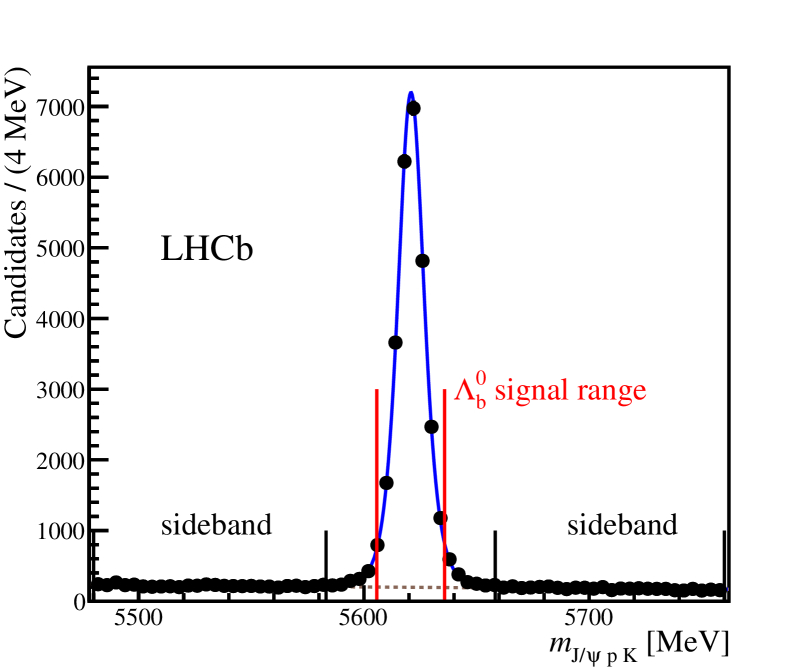
The LHCb detector is a single-arm forward spectrometer covering the pseudorapidity range , described in detail in Ref. [14]. The data selection is described in Ref. [3]. A mass window of ( MeV) around the mass peak is selected, leaving candidates for further analysis, with background fraction () equal to 5.4%. The background is subtracted using candidates from the sidebands, which extend from to from the peak (see the supplemental material).
The aim of this analysis is to assess the level of consistency of the data with the hypothesis that all decays proceed via , , with minimal assumptions about the spin and lineshape of possible contributions. This will be referred to as the null-hypothesis . Here, denotes not only excitations of the baryon, but also nonresonant contributions or excitations of the baryon. The latter contributions are expected to be small[15]. The analysis method is two-dimensional and uses the information contained in the Dalitz variables, , or equivalently in , where is the helicity angle of the system, defined as the angle between the and (or ) directions in the rest frame.
The plane is particularly suited for implementing constraints stemming from the hypothesis by expanding the angular distribution in Legendre polynomials :
where is the efficiency-corrected and background-subtracted signal yield, and is an unnormalized Legendre moment of rank ,
Under the hypothesis, components cannot contribute to moments of rank higher than , where is the highest spin of any contribution at the given value. This requirement sets the appropriate value, which can be deduced from the lightest experimentally known resonances for each , or from the quark model, as in Fig. 1.
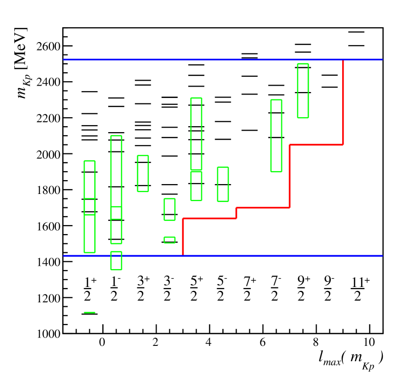
An function is formed, guided by the values of resonance masses () lowered by two units of their widths (): for up to , 5 up to , 7 up to and 9 for higher masses as visualized in Fig. 1.
Reflections from other channels, , or , , would introduce both low and high rank moments (see the supplemental material for an illustration). The narrower the resonance, the narrower the reflection and the higher the rank of Legendre polynomials required to describe such a structure.
Selection criteria and backgrounds can also produce high- structures in the distribution. Therefore, the data are efficiency-corrected and the background is subtracted. Even though testing the hypothesis involves only two dimensions, the selection efficiency has some dependence on the other phase-space dimensions, namely the and helicity angles, as well as angles between the decay plane and the and decay planes. Averaging the efficiency over these additional dimensions () would introduce biases dependent on the exact dynamics of the decays. Therefore, a six-dimensional efficiency correction is used. The efficiency parameterization, , is the same as that used in the amplitude analysis and is described in Sec. 5 of the supplement of Ref. [3].
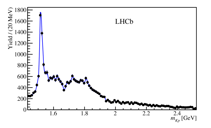
In order to make the analysis as model-independent as possible, no interpretations are imposed on the distribution. Instead, the observed efficiency-corrected and background-subtracted histogram of is used. To obtain a continuous probability density function, , a quadratic interpolation of the histogram is performed, as shown in Fig. 2. The essential part of this analysis method is to incorporate the constraint on the helicity angle distribution: , where is obtained via linear interpolation between neighboring bins of
where is the bin index. Here the Legendre moments are normalized by the yield in the corresponding bin, since the overall normalization of to the data is already contained in the definition. The data are used to determine
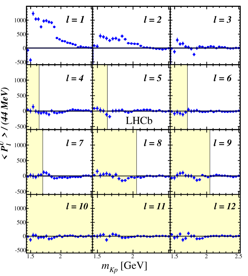
Here the index runs over selected candidates in the signal and sideband regions for the bin of ( is their total number), is the efficiency correction, and is the background subtraction weight, which equals 1 for events in the signal region and for events in the sideband region. Values of are shown in Fig. 3.
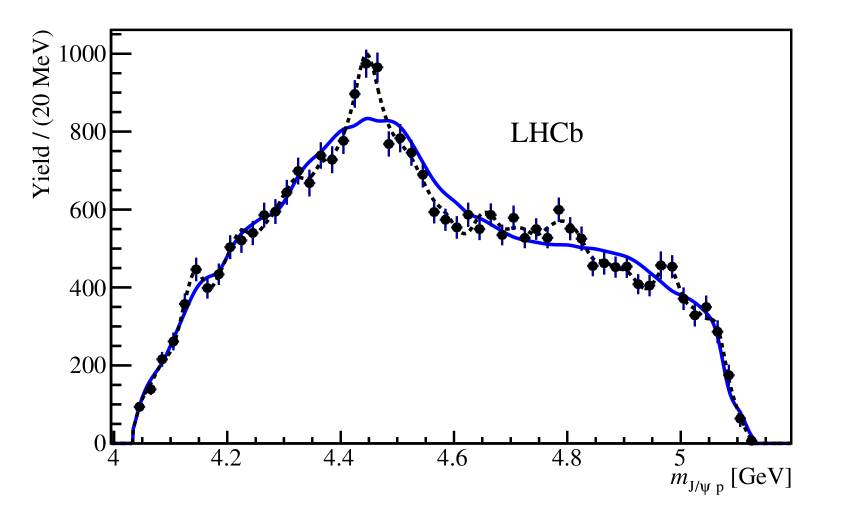
Instead of using the two-dimensional (2D) distribution of to evaluate the consistency of the data with the hypothesis, now expressed by the requirement, it is more convenient to use the () distribution, as any deviations from should appear in the mass region of potential pentaquark (tetraquark) resonances. The projection of onto involves replacing with and integrating over . This integration is carried out numerically, by generating large numbers of simulated events uniformly distributed in and , calculating the corresponding value of , and then filling a histogram with as a weight. In Fig. 4, is compared to the directly obtained efficiency-corrected and background-subtracted distribution in the data.
To probe the compatibility of with the data, a sensitive test can be constructed by making a specific alternative hypothesis (). Following the method discussed in Ref. [13] is defined as , where is not dependent on and large enough to reproduce structures induced by or contributions. The significance of the Legendre moments is probed using the likelihood ratio test:
with normalizations determined via Monte Carlo integration. Note that the explicit event-by-event efficiency factor cancels in the likelihood ratio, but enters the likelihood normalizations. In order for the test to have optimal sensitivity, the value should be set such that the statistically significant features of the data are properly described. Beyond that the power of the test deteriorates. The limit would result in a perfect description of the data, but a weak test since then the test statistic would pick up the fluctuations in the data. For the same reason it is also important to choose independently of the actual data. Here is taken, one unit larger than the value used in the model-independent analysis of [13], as baryons have half-integer spins. The result for is shown in Fig. 4, where it is seen that is sufficient. To make continuous, quadratic splines are used to interpolate between nearby bins.
The numerical representations of and of contain a large number of parameters, requiring extensive statistical simulations to determine the distribution of the test variable for the hypothesis: . A large number of pseudoexperiments are generated with and equal to those obtained in the data. The signal events, contributing a fraction to the signal region sample, are generated according to the function with parameters determined from the data. They are then shaped according to the function, with the angles generated uniformly in phase space. The latter is an approximation, whose possible impact is discussed later. Background events in sideband and signal regions are generated according to the 6D background parameterization previously developed in the amplitude analysis of the same data (Ref. [3] supplement). The pseudoexperiments are subject to the same analysis procedure as the data. The distribution of values of over more than 10 000 pseudoexperiments determines the form of , which can then be used to convert the value obtained from data into a corresponding -value. A small -value indicates non- contributions in the data. A large -value means that the data are consistent with the -only hypothesis, but does not rule out other contributions.
Before applying this method to the data, it is useful to study its sensitivity with the help of amplitude models. Pseudoexperiments are generated according to the 6D amplitude model containing only resonances (the reduced model in Table 1 of Ref. [3]), along with efficiency effects. The distribution of values is close to that expected from (black open and red falling hatched histograms in Fig. 5), thus verifying the 2D model-independent procedure on one example of the model. They also indicate that the non-uniformities in are small enough not to significantly bias the distribution when approximating the probability density via a uniform distribution. To test the sensitivity of the method to an exotic resonance, the amplitude model described in Ref. [3] is used, but with the contribution removed. Generating many pseudoexperiments from this amplitude model produces a distribution of , which is almost indistinguishable from the distribution (blue dotted and red falling hatched histograms in Fig. 5), thus predicting that for such a broad resonance ( ) the false hypothesis is expected to be accepted (type II error), because the contribution inevitably feeds into the numerical representation of . Simulations are then repeated while reducing the width by subsequent factors of two, showing a dramatic increase in the power of the test (histograms peaking at 60 and 300). Figure 5 also shows the distribution obtained with the narrow state restored in the amplitude model and at its nominal width (black rising hatched histogram). The separation from is smaller than that of the simulation with a of comparable width () due to the smaller fit fraction.
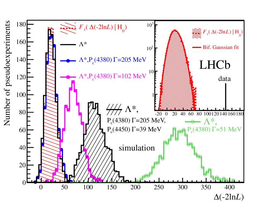
Nevertheless, the separation from is clear; thus, if this amplitude model is a good representation of the data, the hypothesis is expected to essentially always be rejected.
The value of the test variable obtained from the data is significantly above the distribution (see the inset of Fig. 5). To estimate a -value the simulated distribution is fitted with a bifurcated Gaussian function (asymmetric widths); the significance of the rejection is standard deviations.
To test the sensitivity of the result to possible biases from the background subtraction, either the left or the right sideband is exclusively used, and the weakest obtained rejection of is . As a further check, the sideband subtraction is performed with the sPlot technique [16], in which the weights are obtained from the fit to the distribution for candidates in the entire fit range. This increases the significance of the rejection to . Loosening the cut on the boosted decision tree variable discussed in Ref. [3] increases the signal efficiency by 14%, while doubling the background fraction , and causes the significance of the rejection to increase to . Replacing the uniform generation of the angles in the pseudoexperiments with that of the amplitude model without the and states, but generating in the model-independent way, results in a rejection.
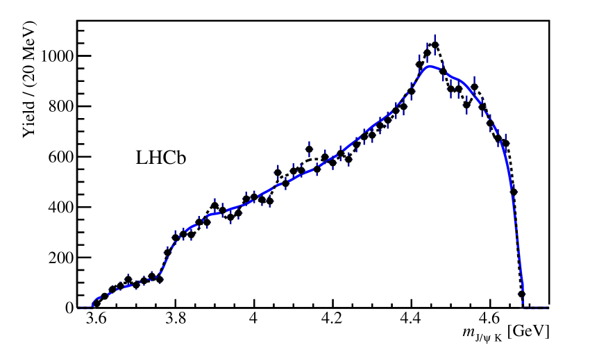
Figure 4 indicates that the rejection of the hypothesis has to do with a narrow peak in the data near . Determination of any parameters is not possible without a model-dependent analysis, because states feed into the numerical representation of in an intractable manner.
The testing is repeated using instead of . The distribution, with and superimposed, is shown in Fig. 6. The test gives a rejection of , which is lower than the rejection obtained using , thus providing model-independent evidence that non- contributions are more likely of the type. Further, in the model-dependent amplitude analysis [3], it was seen that the states reflected into the distribution in the region in which disagrees with the data.
In summary, it has been demonstrated at more than standard deviations that the decays cannot all be attributed to resonant or nonresonant contributions. The analysis requires only minimal assumptions on the mass and spin of the contributions; no assumptions on their number, their resonant or nonresonant nature, or their lineshapes have been made. Non- contributions, which must be present in the data, can be either of the exotic hadron type, or due to rescattering effects among ordinary hadrons. This result supports the amplitude model-dependent observation of the resonances presented previously [3].
We express our gratitude to our colleagues in the CERN accelerator departments for the excellent performance of the LHC. We thank the technical and administrative staff at the LHCb institutes. We acknowledge support from CERN and from the national agencies: CAPES, CNPq, FAPERJ and FINEP (Brazil); NSFC (China); CNRS/IN2P3 (France); BMBF, DFG and MPG (Germany); INFN (Italy); FOM and NWO (The Netherlands); MNiSW and NCN (Poland); MEN/IFA (Romania); MinES and FANO (Russia); MinECo (Spain); SNSF and SER (Switzerland); NASU (Ukraine); STFC (United Kingdom); NSF (USA). We acknowledge the computing resources that are provided by CERN, IN2P3 (France), KIT and DESY (Germany), INFN (Italy), SURF (The Netherlands), PIC (Spain), GridPP (United Kingdom), RRCKI and Yandex LLC (Russia), CSCS (Switzerland), IFIN-HH (Romania), CBPF (Brazil), PL-GRID (Poland) and OSC (USA). We are indebted to the communities behind the multiple open source software packages on which we depend. Individual groups or members have received support from AvH Foundation (Germany), EPLANET, Marie Skłodowska-Curie Actions and ERC (European Union), Conseil Général de Haute-Savoie, Labex ENIGMASS and OCEVU, Région Auvergne (France), RFBR and Yandex LLC (Russia), GVA, XuntaGal and GENCAT (Spain), Herchel Smith Fund, The Royal Society, Royal Commission for the Exhibition of 1851 and the Leverhulme Trust (United Kingdom).
References
- [1] M. Gell-Mann, A schematic model of baryons and mesons, Phys. Lett. 8 (1964) 214
- [2] G. Zweig, An SU3 model for strong interaction symmetry and its breaking, CERN-TH-401, 1964
- [3] LHCb collaboration, R. Aaij et al., Observation of resonances consistent with pentaquark states in decays, Phys. Rev. Lett. 115 (2015) 072001, arXiv:1507.03414
- [4] C. Fernandez-Ramirez et al., Coupled-channel model for scattering in the resonant region, arXiv:1510.07065
- [5] R. N. Faustov and V. O. Galkin, Strange baryon spectroscopy in the relativistic quark model, Phys. Rev. D92 (2015) 054005, arXiv:1507.04530
- [6] S. Capstick and N. Isgur, Baryons in a relativized quark model with chromodynamics, Phys. Rev. D34 (1986) 2809
- [7] U. Loring, B. C. Metsch, and H. R. Petry, The light-baryon spectrum in a relativistic quark model with instanton-induced quark forces, Eur. Phys. J. A10 (2001) 395, arXiv:hep-ph/0103289
- [8] T. Melde, W. Plessas, and B. Sengl, Quark-model identification of baryon ground and resonant states, Phys. Rev. D77 (2008) 114002, arXiv:0806.1454
- [9] E. Santopinto and J. Ferretti, Strange and nonstrange baryon spectra in the relativistic interacting quark-diquark model with a Gürsey and Radicati-inspired exchange interaction, Phys. Rev. C92 (2015) 025202, arXiv:1412.7571
- [10] G. P. Engel, C. B. Lang, D. Mohler, and A. Schaefer, QCD with two light dynamical chirally improved quarks: baryons, Phys. Rev. D87 (2013) 074504, arXiv:1301.4318
- [11] Particle Data Group, K. A. Olive et al., Review of particle physics, Chin. Phys. C38 (2014) 090001, and 2015 update
- [12] BaBar collaboration, B. Aubert et al., Search for the at BaBar, Phys. Rev. D79 (2009) 112001, arXiv:0811.0564
- [13] LHCb collaboration, R. Aaij et al., A model-independent confirmation of the state, Phys. Rev. D92 (2015) 112009, arXiv:1510.01951
- [14] LHCb collaboration, A. A. Alves Jr. et al., The LHCb detector at the LHC, JINST 3 (2008) S08005
- [15] J. F. Donoghue, E. Golowich, W. A. Ponce, and B. R. Holstein, Analysis of S=1 nonleptonic weak decays and the I=1/2 rule, Phys. Rev. D21 (1980) 186
- [16] M. Pivk and F. R. Le Diberder, sPlot: A statistical tool to unfold data distributions, Nucl. Instrum. Meth. A555 (2005) 356, arXiv:physics/0402083v3
Appendix: Supplemental material
1 Data sample
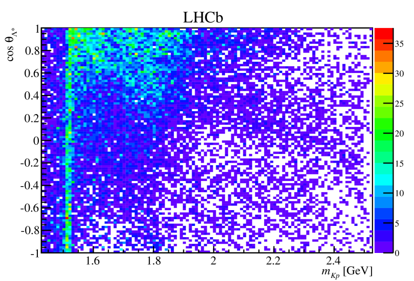
The definition of the signal and sideband regions is illustrated in Fig. 7. The background-subtracted and efficiency-corrected distribution of the data on the rectangular Dalitz plane is shown in Fig. 8.
2 Simulations based on amplitude models
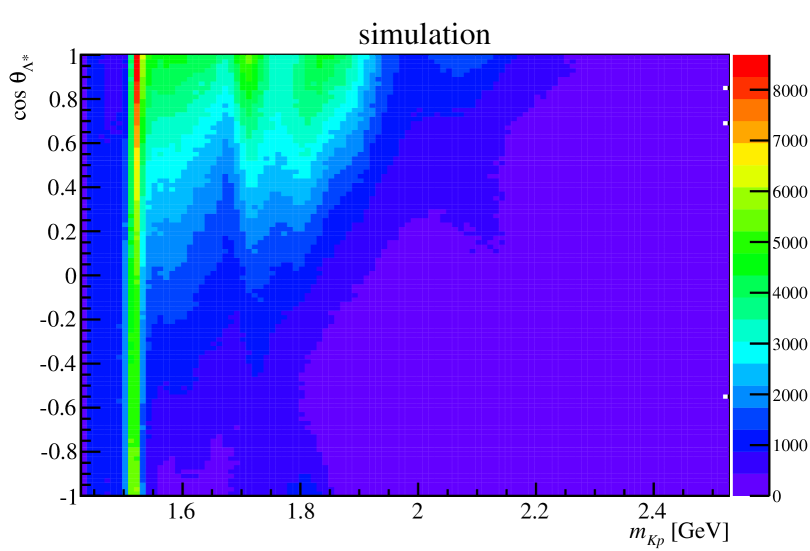
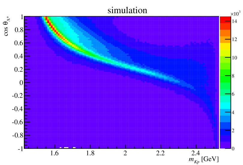
The rectangular Dalitz plane distributions for the large statistics pseudo-samples generated from the amplitude model with only the resonances and from the amplitude model with only the and resonances are shown in Figs. 9 and 10, respectively. Parameters of the models, without and with the states, were determined by fitting the amplitude models to the data as described in Ref. [3].
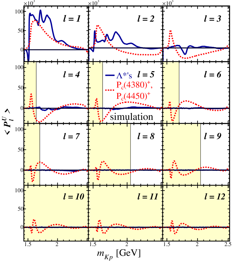
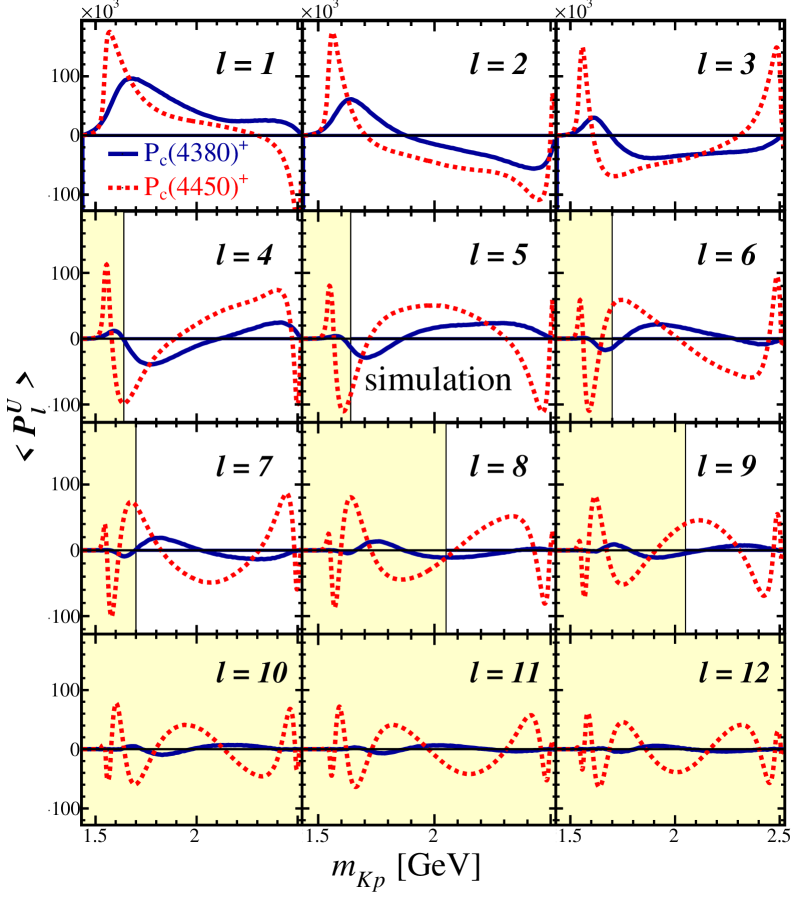
The Legendre moments of distributions () in various bins of are compared between these two simulated pseudo-samples in Fig. 11. The filter, used in forming a numerical representation of the hypothesis that only contributions are present (), is also illustrated in Fig. 11: moments in the shaded regions () are neglected. The pentaquark resonances can induce significant values of the moments in these regions, as illustrated with the example amplitude model containing only states. The states also contribute significantly to the unshaded regions, thus feeding into the numerical representation of the hypothesis, and decreasing the sensitivity of the model-independent approach to exotic hadron contributions. This is especially true for wide resonances, which contribute very little to high moments, as illustrated for the state in Fig. 12. The example amplitude model with only resonances contributes to the unshaded regions only, as expected.
LHCb collaboration
R. Aaij39,
C. Abellán Beteta41,
B. Adeva38,
M. Adinolfi47,
Z. Ajaltouni5,
S. Akar6,
J. Albrecht10,
F. Alessio39,
M. Alexander52,
S. Ali42,
G. Alkhazov31,
P. Alvarez Cartelle54,
A.A. Alves Jr58,
S. Amato2,
S. Amerio23,
Y. Amhis7,
L. An3,40,
L. Anderlini18,
G. Andreassi40,
M. Andreotti17,g,
J.E. Andrews59,
R.B. Appleby55,
O. Aquines Gutierrez11,
F. Archilli39,
P. d’Argent12,
A. Artamonov36,
M. Artuso60,
E. Aslanides6,
G. Auriemma26,n,
M. Baalouch5,
S. Bachmann12,
J.J. Back49,
A. Badalov37,
C. Baesso61,
S. Baker54,
W. Baldini17,
R.J. Barlow55,
C. Barschel39,
S. Barsuk7,
W. Barter39,
V. Batozskaya29,
V. Battista40,
A. Bay40,
L. Beaucourt4,
J. Beddow52,
F. Bedeschi24,
I. Bediaga1,
L.J. Bel42,
V. Bellee40,
N. Belloli21,k,
I. Belyaev32,
E. Ben-Haim8,
G. Bencivenni19,
S. Benson39,
J. Benton47,
A. Berezhnoy33,
R. Bernet41,
A. Bertolin23,
F. Betti15,
M.-O. Bettler39,
M. van Beuzekom42,
S. Bifani46,
P. Billoir8,
T. Bird55,
A. Birnkraut10,
A. Bizzeti18,i,
T. Blake49,
F. Blanc40,
J. Blouw11,
S. Blusk60,
V. Bocci26,
A. Bondar35,
N. Bondar31,39,
W. Bonivento16,
A. Borgheresi21,k,
S. Borghi55,
M. Borisyak67,
M. Borsato38,
M. Boubdir9,
T.J.V. Bowcock53,
E. Bowen41,
C. Bozzi17,39,
S. Braun12,
M. Britsch12,
T. Britton60,
J. Brodzicka55,
E. Buchanan47,
C. Burr55,
A. Bursche2,
J. Buytaert39,
S. Cadeddu16,
R. Calabrese17,g,
M. Calvi21,k,
M. Calvo Gomez37,p,
P. Campana19,
D. Campora Perez39,
L. Capriotti55,
A. Carbone15,e,
G. Carboni25,l,
R. Cardinale20,j,
A. Cardini16,
P. Carniti21,k,
L. Carson51,
K. Carvalho Akiba2,
G. Casse53,
L. Cassina21,k,
L. Castillo Garcia40,
M. Cattaneo39,
Ch. Cauet10,
G. Cavallero20,
R. Cenci24,t,
M. Charles8,
Ph. Charpentier39,
G. Chatzikonstantinidis46,
M. Chefdeville4,
S. Chen55,
S.-F. Cheung56,
V. Chobanova38,
M. Chrzaszcz41,27,
X. Cid Vidal39,
G. Ciezarek42,
P.E.L. Clarke51,
M. Clemencic39,
H.V. Cliff48,
J. Closier39,
V. Coco58,
J. Cogan6,
E. Cogneras5,
V. Cogoni16,f,
L. Cojocariu30,
G. Collazuol23,r,
P. Collins39,
A. Comerma-Montells12,
A. Contu39,
A. Cook47,
S. Coquereau8,
G. Corti39,
M. Corvo17,g,
B. Couturier39,
G.A. Cowan51,
D.C. Craik51,
A. Crocombe49,
M. Cruz Torres61,
S. Cunliffe54,
R. Currie54,
C. D’Ambrosio39,
E. Dall’Occo42,
J. Dalseno47,
P.N.Y. David42,
A. Davis58,
O. De Aguiar Francisco2,
K. De Bruyn6,
S. De Capua55,
M. De Cian12,
J.M. De Miranda1,
L. De Paula2,
P. De Simone19,
C.-T. Dean52,
D. Decamp4,
M. Deckenhoff10,
L. Del Buono8,
N. Déléage4,
M. Demmer10,
A. Dendek28,
D. Derkach67,
O. Deschamps5,
F. Dettori39,
B. Dey22,
A. Di Canto39,
H. Dijkstra39,
F. Dordei39,
M. Dorigo40,
A. Dosil Suárez38,
A. Dovbnya44,
K. Dreimanis53,
L. Dufour42,
G. Dujany55,
K. Dungs39,
P. Durante39,
R. Dzhelyadin36,
A. Dziurda39,
A. Dzyuba31,
S. Easo50,39,
U. Egede54,
V. Egorychev32,
S. Eidelman35,
S. Eisenhardt51,
U. Eitschberger10,
R. Ekelhof10,
L. Eklund52,
I. El Rifai5,
Ch. Elsasser41,
S. Ely60,
S. Esen12,
H.M. Evans48,
T. Evans56,
A. Falabella15,
C. Färber39,
N. Farley46,
S. Farry53,
R. Fay53,
D. Fazzini21,k,
D. Ferguson51,
V. Fernandez Albor38,
F. Ferrari15,39,
F. Ferreira Rodrigues1,
M. Ferro-Luzzi39,
S. Filippov34,
M. Fiore17,g,
M. Fiorini17,g,
M. Firlej28,
C. Fitzpatrick40,
T. Fiutowski28,
F. Fleuret7,b,
K. Fohl39,
M. Fontana16,
F. Fontanelli20,j,
D. C. Forshaw60,
R. Forty39,
M. Frank39,
C. Frei39,
M. Frosini18,
J. Fu22,
E. Furfaro25,l,
A. Gallas Torreira38,
D. Galli15,e,
S. Gallorini23,
S. Gambetta51,
M. Gandelman2,
P. Gandini56,
Y. Gao3,
J. García Pardiñas38,
J. Garra Tico48,
L. Garrido37,
P.J. Garsed48,
D. Gascon37,
C. Gaspar39,
L. Gavardi10,
G. Gazzoni5,
D. Gerick12,
E. Gersabeck12,
M. Gersabeck55,
T. Gershon49,
Ph. Ghez4,
S. Gianì40,
V. Gibson48,
O.G. Girard40,
L. Giubega30,
V.V. Gligorov8,
C. Göbel61,
D. Golubkov32,
A. Golutvin54,39,
A. Gomes1,a,
C. Gotti21,k,
M. Grabalosa Gándara5,
R. Graciani Diaz37,
L.A. Granado Cardoso39,
E. Graugés37,
E. Graverini41,
G. Graziani18,
A. Grecu30,
P. Griffith46,
L. Grillo12,
O. Grünberg65,
E. Gushchin34,
Yu. Guz36,39,
T. Gys39,
T. Hadavizadeh56,
C. Hadjivasiliou60,
G. Haefeli40,
C. Haen39,
S.C. Haines48,
S. Hall54,
B. Hamilton59,
X. Han12,
S. Hansmann-Menzemer12,
N. Harnew56,
S.T. Harnew47,
J. Harrison55,
J. He39,
T. Head40,
A. Heister9,
K. Hennessy53,
P. Henrard5,
L. Henry8,
J.A. Hernando Morata38,
E. van Herwijnen39,
M. Heß65,
A. Hicheur2,
D. Hill56,
M. Hoballah5,
C. Hombach55,
L. Hongming40,
W. Hulsbergen42,
T. Humair54,
M. Hushchyn67,
N. Hussain56,
D. Hutchcroft53,
M. Idzik28,
P. Ilten57,
R. Jacobsson39,
A. Jaeger12,
J. Jalocha56,
E. Jans42,
A. Jawahery59,
M. John56,
D. Johnson39,
C.R. Jones48,
C. Joram39,
B. Jost39,
N. Jurik60,
S. Kandybei44,
W. Kanso6,
M. Karacson39,
T.M. Karbach39,†,
S. Karodia52,
M. Kecke12,
M. Kelsey60,
I.R. Kenyon46,
M. Kenzie39,
T. Ketel43,
E. Khairullin67,
B. Khanji21,39,k,
C. Khurewathanakul40,
T. Kirn9,
S. Klaver55,
K. Klimaszewski29,
M. Kolpin12,
I. Komarov40,
R.F. Koopman43,
P. Koppenburg42,
M. Kozeiha5,
L. Kravchuk34,
K. Kreplin12,
M. Kreps49,
P. Krokovny35,
F. Kruse10,
W. Krzemien29,
W. Kucewicz27,o,
M. Kucharczyk27,
V. Kudryavtsev35,
A. K. Kuonen40,
K. Kurek29,
T. Kvaratskheliya32,
D. Lacarrere39,
G. Lafferty55,39,
A. Lai16,
D. Lambert51,
G. Lanfranchi19,
C. Langenbruch49,
B. Langhans39,
T. Latham49,
C. Lazzeroni46,
R. Le Gac6,
J. van Leerdam42,
J.-P. Lees4,
R. Lefèvre5,
A. Leflat33,39,
J. Lefrançois7,
F. Lemaitre39,
E. Lemos Cid38,
O. Leroy6,
T. Lesiak27,
B. Leverington12,
Y. Li7,
T. Likhomanenko67,66,
R. Lindner39,
C. Linn39,
F. Lionetto41,
B. Liu16,
X. Liu3,
D. Loh49,
I. Longstaff52,
J.H. Lopes2,
D. Lucchesi23,r,
M. Lucio Martinez38,
H. Luo51,
A. Lupato23,
E. Luppi17,g,
O. Lupton56,
N. Lusardi22,
A. Lusiani24,
X. Lyu62,
F. Machefert7,
F. Maciuc30,
O. Maev31,
K. Maguire55,
S. Malde56,
A. Malinin66,
G. Manca7,
G. Mancinelli6,
P. Manning60,
A. Mapelli39,
J. Maratas5,
J.F. Marchand4,
U. Marconi15,
C. Marin Benito37,
P. Marino24,t,
J. Marks12,
G. Martellotti26,
M. Martin6,
M. Martinelli40,
D. Martinez Santos38,
F. Martinez Vidal68,
D. Martins Tostes2,
L.M. Massacrier7,
A. Massafferri1,
R. Matev39,
A. Mathad49,
Z. Mathe39,
C. Matteuzzi21,
A. Mauri41,
B. Maurin40,
A. Mazurov46,
M. McCann54,
J. McCarthy46,
A. McNab55,
R. McNulty13,
B. Meadows58,
F. Meier10,
M. Meissner12,
D. Melnychuk29,
M. Merk42,
A Merli22,u,
E Michielin23,
D.A. Milanes64,
M.-N. Minard4,
D.S. Mitzel12,
J. Molina Rodriguez61,
I.A. Monroy64,
S. Monteil5,
M. Morandin23,
P. Morawski28,
A. Mordà6,
M.J. Morello24,t,
J. Moron28,
A.B. Morris51,
R. Mountain60,
F. Muheim51,
MM Mulder42,
D. Müller55,
J. Müller10,
K. Müller41,
V. Müller10,
M. Mussini15,
B. Muster40,
P. Naik47,
T. Nakada40,
R. Nandakumar50,
A. Nandi56,
I. Nasteva2,
M. Needham51,
N. Neri22,
S. Neubert12,
N. Neufeld39,
M. Neuner12,
A.D. Nguyen40,
C. Nguyen-Mau40,q,
V. Niess5,
S. Nieswand9,
R. Niet10,
N. Nikitin33,
T. Nikodem12,
A. Novoselov36,
D.P. O’Hanlon49,
A. Oblakowska-Mucha28,
V. Obraztsov36,
S. Ogilvy19,
O. Okhrimenko45,
R. Oldeman16,48,f,
C.J.G. Onderwater69,
B. Osorio Rodrigues1,
J.M. Otalora Goicochea2,
A. Otto39,
P. Owen54,
A. Oyanguren68,
A. Palano14,d,
F. Palombo22,u,
M. Palutan19,
J. Panman39,
A. Papanestis50,
M. Pappagallo52,
L.L. Pappalardo17,g,
C. Pappenheimer58,
W. Parker59,
C. Parkes55,
G. Passaleva18,
G.D. Patel53,
M. Patel54,
C. Patrignani20,j,
A. Pearce55,50,
A. Pellegrino42,
G. Penso26,m,
M. Pepe Altarelli39,
S. Perazzini39,
P. Perret5,
L. Pescatore46,
K. Petridis47,
A. Petrolini20,j,
M. Petruzzo22,
E. Picatoste Olloqui37,
B. Pietrzyk4,
M. Pikies27,
D. Pinci26,
A. Pistone20,
A. Piucci12,
S. Playfer51,
M. Plo Casasus38,
T. Poikela39,
F. Polci8,
A. Poluektov49,35,
I. Polyakov32,
E. Polycarpo2,
A. Popov36,
D. Popov11,39,
B. Popovici30,
C. Potterat2,
E. Price47,
J.D. Price53,
J. Prisciandaro38,
A. Pritchard53,
C. Prouve47,
V. Pugatch45,
A. Puig Navarro40,
G. Punzi24,s,
W. Qian56,
R. Quagliani7,47,
B. Rachwal27,
J.H. Rademacker47,
M. Rama24,
M. Ramos Pernas38,
M.S. Rangel2,
I. Raniuk44,
G. Raven43,
F. Redi54,
S. Reichert10,
A.C. dos Reis1,
V. Renaudin7,
S. Ricciardi50,
S. Richards47,
M. Rihl39,
K. Rinnert53,39,
V. Rives Molina37,
P. Robbe7,
A.B. Rodrigues1,
E. Rodrigues58,
J.A. Rodriguez Lopez64,
P. Rodriguez Perez55,
A. Rogozhnikov67,
S. Roiser39,
V. Romanovsky36,
A. Romero Vidal38,
J. W. Ronayne13,
M. Rotondo23,
T. Ruf39,
P. Ruiz Valls68,
J.J. Saborido Silva38,
N. Sagidova31,
B. Saitta16,f,
V. Salustino Guimaraes2,
C. Sanchez Mayordomo68,
B. Sanmartin Sedes38,
R. Santacesaria26,
C. Santamarina Rios38,
M. Santimaria19,
E. Santovetti25,l,
A. Sarti19,m,
C. Satriano26,n,
A. Satta25,
D.M. Saunders47,
D. Savrina32,33,
S. Schael9,
M. Schiller39,
H. Schindler39,
M. Schlupp10,
M. Schmelling11,
T. Schmelzer10,
B. Schmidt39,
O. Schneider40,
A. Schopper39,
M. Schubiger40,
M.-H. Schune7,
R. Schwemmer39,
B. Sciascia19,
A. Sciubba26,m,
A. Semennikov32,
A. Sergi46,
N. Serra41,
J. Serrano6,
L. Sestini23,
P. Seyfert21,
M. Shapkin36,
I. Shapoval17,44,g,
Y. Shcheglov31,
T. Shears53,
L. Shekhtman35,
V. Shevchenko66,
A. Shires10,
B.G. Siddi17,
R. Silva Coutinho41,
L. Silva de Oliveira2,
G. Simi23,s,
M. Sirendi48,
N. Skidmore47,
T. Skwarnicki60,
E. Smith54,
I.T. Smith51,
J. Smith48,
M. Smith55,
H. Snoek42,
M.D. Sokoloff58,
F.J.P. Soler52,
F. Soomro40,
D. Souza47,
B. Souza De Paula2,
B. Spaan10,
P. Spradlin52,
S. Sridharan39,
F. Stagni39,
M. Stahl12,
S. Stahl39,
S. Stefkova54,
O. Steinkamp41,
O. Stenyakin36,
S. Stevenson56,
S. Stoica30,
S. Stone60,
B. Storaci41,
S. Stracka24,t,
M. Straticiuc30,
U. Straumann41,
L. Sun58,
W. Sutcliffe54,
K. Swientek28,
S. Swientek10,
V. Syropoulos43,
M. Szczekowski29,
T. Szumlak28,
S. T’Jampens4,
A. Tayduganov6,
T. Tekampe10,
G. Tellarini17,g,
F. Teubert39,
C. Thomas56,
E. Thomas39,
J. van Tilburg42,
V. Tisserand4,
M. Tobin40,
S. Tolk43,
L. Tomassetti17,g,
D. Tonelli39,
S. Topp-Joergensen56,
E. Tournefier4,
S. Tourneur40,
K. Trabelsi40,
M. Traill52,
M.T. Tran40,
M. Tresch41,
A. Trisovic39,
A. Tsaregorodtsev6,
P. Tsopelas42,
N. Tuning42,39,
A. Ukleja29,
A. Ustyuzhanin67,66,
U. Uwer12,
C. Vacca16,39,f,
V. Vagnoni15,39,
S. Valat39,
G. Valenti15,
A. Vallier7,
R. Vazquez Gomez19,
P. Vazquez Regueiro38,
C. Vázquez Sierra38,
S. Vecchi17,
M. van Veghel42,
J.J. Velthuis47,
M. Veltri18,h,
G. Veneziano40,
M. Vesterinen12,
B. Viaud7,
D. Vieira2,
M. Vieites Diaz38,
X. Vilasis-Cardona37,p,
V. Volkov33,
A. Vollhardt41,
D. Voong47,
A. Vorobyev31,
V. Vorobyev35,
C. Voß65,
J.A. de Vries42,
R. Waldi65,
C. Wallace49,
R. Wallace13,
J. Walsh24,
J. Wang60,
D.R. Ward48,
N.K. Watson46,
D. Websdale54,
A. Weiden41,
M. Whitehead39,
J. Wicht49,
G. Wilkinson56,39,
M. Wilkinson60,
M. Williams39,
M.P. Williams46,
M. Williams57,
T. Williams46,
F.F. Wilson50,
J. Wimberley59,
J. Wishahi10,
W. Wislicki29,
M. Witek27,
G. Wormser7,
S.A. Wotton48,
K. Wraight52,
S. Wright48,
K. Wyllie39,
Y. Xie63,
Z. Xu40,
Z. Yang3,
H. Yin63,
J. Yu63,
X. Yuan35,
O. Yushchenko36,
M. Zangoli15,
M. Zavertyaev11,c,
L. Zhang3,
Y. Zhang7,
A. Zhelezov12,
Y. Zheng62,
A. Zhokhov32,
L. Zhong3,
V. Zhukov9,
S. Zucchelli15.
1Centro Brasileiro de Pesquisas Físicas (CBPF), Rio de Janeiro, Brazil
2Universidade Federal do Rio de Janeiro (UFRJ), Rio de Janeiro, Brazil
3Center for High Energy Physics, Tsinghua University, Beijing, China
4LAPP, Université Savoie Mont-Blanc, CNRS/IN2P3, Annecy-Le-Vieux, France
5Clermont Université, Université Blaise Pascal, CNRS/IN2P3, LPC, Clermont-Ferrand, France
6CPPM, Aix-Marseille Université, CNRS/IN2P3, Marseille, France
7LAL, Université Paris-Sud, CNRS/IN2P3, Orsay, France
8LPNHE, Université Pierre et Marie Curie, Université Paris Diderot, CNRS/IN2P3, Paris, France
9I. Physikalisches Institut, RWTH Aachen University, Aachen, Germany
10Fakultät Physik, Technische Universität Dortmund, Dortmund, Germany
11Max-Planck-Institut für Kernphysik (MPIK), Heidelberg, Germany
12Physikalisches Institut, Ruprecht-Karls-Universität Heidelberg, Heidelberg, Germany
13School of Physics, University College Dublin, Dublin, Ireland
14Sezione INFN di Bari, Bari, Italy
15Sezione INFN di Bologna, Bologna, Italy
16Sezione INFN di Cagliari, Cagliari, Italy
17Sezione INFN di Ferrara, Ferrara, Italy
18Sezione INFN di Firenze, Firenze, Italy
19Laboratori Nazionali dell’INFN di Frascati, Frascati, Italy
20Sezione INFN di Genova, Genova, Italy
21Sezione INFN di Milano Bicocca, Milano, Italy
22Sezione INFN di Milano, Milano, Italy
23Sezione INFN di Padova, Padova, Italy
24Sezione INFN di Pisa, Pisa, Italy
25Sezione INFN di Roma Tor Vergata, Roma, Italy
26Sezione INFN di Roma La Sapienza, Roma, Italy
27Henryk Niewodniczanski Institute of Nuclear Physics Polish Academy of Sciences, Kraków, Poland
28AGH - University of Science and Technology, Faculty of Physics and Applied Computer Science, Kraków, Poland
29National Center for Nuclear Research (NCBJ), Warsaw, Poland
30Horia Hulubei National Institute of Physics and Nuclear Engineering, Bucharest-Magurele, Romania
31Petersburg Nuclear Physics Institute (PNPI), Gatchina, Russia
32Institute of Theoretical and Experimental Physics (ITEP), Moscow, Russia
33Institute of Nuclear Physics, Moscow State University (SINP MSU), Moscow, Russia
34Institute for Nuclear Research of the Russian Academy of Sciences (INR RAN), Moscow, Russia
35Budker Institute of Nuclear Physics (SB RAS) and Novosibirsk State University, Novosibirsk, Russia
36Institute for High Energy Physics (IHEP), Protvino, Russia
37Universitat de Barcelona, Barcelona, Spain
38Universidad de Santiago de Compostela, Santiago de Compostela, Spain
39European Organization for Nuclear Research (CERN), Geneva, Switzerland
40Ecole Polytechnique Fédérale de Lausanne (EPFL), Lausanne, Switzerland
41Physik-Institut, Universität Zürich, Zürich, Switzerland
42Nikhef National Institute for Subatomic Physics, Amsterdam, The Netherlands
43Nikhef National Institute for Subatomic Physics and VU University Amsterdam, Amsterdam, The Netherlands
44NSC Kharkiv Institute of Physics and Technology (NSC KIPT), Kharkiv, Ukraine
45Institute for Nuclear Research of the National Academy of Sciences (KINR), Kyiv, Ukraine
46University of Birmingham, Birmingham, United Kingdom
47H.H. Wills Physics Laboratory, University of Bristol, Bristol, United Kingdom
48Cavendish Laboratory, University of Cambridge, Cambridge, United Kingdom
49Department of Physics, University of Warwick, Coventry, United Kingdom
50STFC Rutherford Appleton Laboratory, Didcot, United Kingdom
51School of Physics and Astronomy, University of Edinburgh, Edinburgh, United Kingdom
52School of Physics and Astronomy, University of Glasgow, Glasgow, United Kingdom
53Oliver Lodge Laboratory, University of Liverpool, Liverpool, United Kingdom
54Imperial College London, London, United Kingdom
55School of Physics and Astronomy, University of Manchester, Manchester, United Kingdom
56Department of Physics, University of Oxford, Oxford, United Kingdom
57Massachusetts Institute of Technology, Cambridge, MA, United States
58University of Cincinnati, Cincinnati, OH, United States
59University of Maryland, College Park, MD, United States
60Syracuse University, Syracuse, NY, United States
61Pontifícia Universidade Católica do Rio de Janeiro (PUC-Rio), Rio de Janeiro, Brazil, associated to 2
62University of Chinese Academy of Sciences, Beijing, China, associated to 3
63Institute of Particle Physics, Central China Normal University, Wuhan, Hubei, China, associated to 3
64Departamento de Fisica , Universidad Nacional de Colombia, Bogota, Colombia, associated to 8
65Institut für Physik, Universität Rostock, Rostock, Germany, associated to 12
66National Research Centre Kurchatov Institute, Moscow, Russia, associated to 32
67Yandex School of Data Analysis, Moscow, Russia, associated to 32
68Instituto de Fisica Corpuscular (IFIC), Universitat de Valencia-CSIC, Valencia, Spain, associated to 37
69Van Swinderen Institute, University of Groningen, Groningen, The Netherlands, associated to 42
aUniversidade Federal do Triângulo Mineiro (UFTM), Uberaba-MG, Brazil
bLaboratoire Leprince-Ringuet, Palaiseau, France
cP.N. Lebedev Physical Institute, Russian Academy of Science (LPI RAS), Moscow, Russia
dUniversità di Bari, Bari, Italy
eUniversità di Bologna, Bologna, Italy
fUniversità di Cagliari, Cagliari, Italy
gUniversità di Ferrara, Ferrara, Italy
hUniversità di Urbino, Urbino, Italy
iUniversità di Modena e Reggio Emilia, Modena, Italy
jUniversità di Genova, Genova, Italy
kUniversità di Milano Bicocca, Milano, Italy
lUniversità di Roma Tor Vergata, Roma, Italy
mUniversità di Roma La Sapienza, Roma, Italy
nUniversità della Basilicata, Potenza, Italy
oAGH - University of Science and Technology, Faculty of Computer Science, Electronics and Telecommunications, Kraków, Poland
pLIFAELS, La Salle, Universitat Ramon Llull, Barcelona, Spain
qHanoi University of Science, Hanoi, Viet Nam
rUniversità di Padova, Padova, Italy
sUniversità di Pisa, Pisa, Italy
tScuola Normale Superiore, Pisa, Italy
uUniversità degli Studi di Milano, Milano, Italy
†Deceased