Remark on Structure of Expectation Values of Flavor-Lepton Numbers with respect to Neutrino-Source Hadron States:
Deviation from Fermi’s Golden Relation

Kanji Fujii1 and Norihito Toyota2        1)Department of Physics, Faculty of Science, Hokkaido University,
Sapporo 060-0810, Japan
   2)Faculty of Business Administration and Information Science,
       Hokkaido Information University, Ebetsu, Nisinopporo 59-2, Japan
fujii@particle.sci.hokudai.ac.jp, toyota@do-johodai.ac.jp
Abstract

In our preceeding reports, we have pointed out that a unified description of weak decays accompanying neutrinos and the oscillation process is obtained on the basis of the expectation values of flavor-neutrino numbers with respect to the neutrino-source hadron state. In the present report, we investigate the effect on the expectation values due to the deviation from Fermi’s golden relation, and give concrete features of these deviations in the case of π+superscript𝜋\pi^{+} and K+superscript𝐾K^{+}-decays under the simple situation with the 333-momentum pA=0subscript𝑝𝐴0\vec{p_{A}}=0 for A=π+𝐴superscript𝜋A=\pi^{+}, K+superscript𝐾K^{+}.

1 Introduction

1.1 Purpose

It has been pointed out in the preceeding papers Ref.[1, 2, 3] that a unified description of the weak decays accompanied by neutrinos as well as the neutrino-oscillation process is obtained when we consider the expectation values of the flavor-lepton numbers with respect to neutrino-source hadron state A𝐴A. (In Ref.[3] and also in the following we consider mainly the cases A=π+𝐴superscript𝜋A=\pi^{+} and K+superscript𝐾K^{+}.)

From the expectation-value approach, we obtain the quantities which are natutally interpreted as the decay probabilities where the neutrino-mixing exists, and also the quantities as the neutrino-oscillation formulas.

Being motivated by Ref.[4], we have considered in Ref.[3] the ration X1/X2subscript𝑋1subscript𝑋2X_{1}/X_{2} of the two relevant quantities X1subscript𝑋1X_{1} and X2subscript𝑋2X_{2} in order to see the situation how Fermi’s golden relation holds. In the following, after remembering the structures of the ration X1/X2subscript𝑋1subscript𝑋2X_{1}/X_{2} given in Ref. [3], we examine the difference X1X2subscript𝑋1subscript𝑋2X_{1}-X_{2} between those two relevant quantities; the difference X1X2subscript𝑋1subscript𝑋2X_{1}-X_{2} corresponds to the difference examined in Ref.[4], and the these two kinds of quantities, X1/X2subscript𝑋1subscript𝑋2X_{1}/X_{2} and X1X2subscript𝑋1subscript𝑋2X_{1}-X_{2} are simply related with each other through the fundamental arithmetic operations. This situation is to be confirmed through numerical calculations.

1.2 Definitions of relevant quantities

In this subsection we summarize the definitions of relevant quantities, which are used in our preceding work Ref.[3].

The lowest-order contribution to the expectation values of charged-lepton number Nσ(x0)subscript𝑁𝜎superscript𝑥0N_{\ell\sigma}(x^{0}) mainly comes from the expectation value

Nσ,A+;x0,xI0I=A+(x0)|xI0x0d4yxI0x0d4zHint(z)Nσ(x0)Hint(y)|A+(xI0).subscriptsubscript𝑁subscript𝜎superscript𝐴superscript𝑥0superscriptsubscript𝑥𝐼0𝐼quantum-operator-productsuperscript𝐴superscript𝑥0superscriptsubscriptsuperscriptsubscript𝑥𝐼0superscript𝑥0superscript𝑑4𝑦superscriptsubscriptsuperscriptsubscript𝑥𝐼0superscript𝑥0superscript𝑑4𝑧subscript𝐻𝑖𝑛𝑡𝑧subscript𝑁subscript𝜎superscript𝑥0subscript𝐻𝑖𝑛𝑡𝑦superscript𝐴superscriptsubscript𝑥𝐼0\langle N_{\ell_{\sigma}},A^{+};x^{0},x_{I}^{0}\rangle_{I}=\langle A^{+}(x^{0})|\int_{x_{I}^{0}}^{x^{0}}d^{4}y\int_{x_{I}^{0}}^{x^{0}}d^{4}zH_{int}(z)N_{\ell_{\sigma}}(x^{0})H_{int}(y)|A^{+}(x_{I}^{0})\rangle. (1)

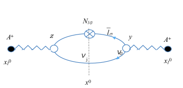
The dominant contribution comes from the diagram shown by Fig.1.
Refer to caption
Figure 1: Dominant contribution to Nσ,A+(p);x0,xI0subscript𝑁𝜎superscript𝐴𝑝superscript𝑥0superscriptsubscript𝑥𝐼0\langle N_{\ell\sigma},A^{+}(p);x^{0},x_{I}^{0}\rangle. This diagram is the same as Fig.2 in Ref.[3].

We write this dominant contribution as n¯σ,A+(p);x0xI0=Tdelimited-⟨⟩subscript¯𝑛subscript𝜎superscript𝐴𝑝superscript𝑥0superscriptsubscript𝑥𝐼0𝑇-\langle\bar{n}_{\ell_{\sigma}},A^{+}(p);x^{0}-x_{I}^{0}=T\rangle. Concretely we obtain the the absolute value of the expectation value of ¯σsubscript¯𝜎\bar{\ell}_{\sigma}-number

n¯σ,A+(p);x0xI0=T[GFfA2]212EA(p)Vqkδ(p,k+q)delimited-⟨⟩subscript¯𝑛𝜎superscript𝐴𝑝superscript𝑥0superscriptsubscript𝑥𝐼0𝑇superscriptdelimited-[]subscript𝐺𝐹subscript𝑓𝐴2212subscript𝐸𝐴𝑝𝑉subscript𝑞subscript𝑘𝛿𝑝𝑘𝑞\displaystyle\langle\bar{n}_{\ell\sigma},A^{+}(p);x^{0}-x_{I}^{0}=T\rangle\cong\Bigl{[}\frac{G_{F}f_{A}}{\sqrt{2}}\Bigr{]}^{2}\frac{1}{2E_{A}(p)V}\sum_{\vec{q}}\sum_{\vec{k}}\delta(\vec{p},\vec{k}+\vec{q})
×jZσj12Zσj12R(jjk,σq,p)[sin(T(EA(p)Eσ(q)ωj(k))/2)(EA(p)Eσ(q)ωj)/2]2,\displaystyle\times\sum_{j}Z_{\sigma j}^{\frac{1}{2}}Z_{\sigma j}^{\frac{1}{2}*}R(jjk,\sigma q,p)\Bigl{[}\frac{\sin(T(E_{A}(p)-E_{\sigma}(q)-\omega_{j}(k))/2)}{(E_{A}(p)-E_{\sigma}(q)-\omega_{j})/2}\Bigr{]}^{2}, (2)

where

R(jjk,σq,p)=2ωj(k)Eσ(q)[mA2(k(j)q)+2(qp)(k(j)p)];𝑅𝑗𝑗𝑘𝜎𝑞𝑝2subscript𝜔𝑗𝑘subscript𝐸𝜎𝑞delimited-[]superscriptsubscript𝑚𝐴2superscript𝑘𝑗𝑞2𝑞𝑝superscript𝑘𝑗𝑝R(jjk,\sigma q,p)=\frac{2}{\omega_{j}(k)E_{\sigma}(q)}\big{[}m_{A}^{2}(k^{(j)}\cdot q)+2(q\cdot p)(k^{(j)}\cdot p)\big{]};

with the notation (k(j)q)=kqωj(k)Eσ(q)superscript𝑘𝑗𝑞𝑘𝑞subscript𝜔𝑗𝑘subscript𝐸𝜎𝑞(k^{(j)}\cdot q)=\vec{k}\vec{q}-\omega_{j}(k)E_{\sigma}(q) and the neutrino-mixing matrix [Zσj12]delimited-[]superscriptsubscript𝑍𝜎𝑗12\big{[}Z_{\sigma j}^{\frac{1}{2}}\big{]}, appearing in the relation between the flavor- and mass-neutrino fields, i.e.formulae-sequence𝑖𝑒i.e. νρ(x)=j=13Zρj12νj(x)subscript𝜈𝜌𝑥superscriptsubscript𝑗13superscriptsubscript𝑍𝜌𝑗12subscript𝜈𝑗𝑥\nu_{\rho}(x)=\sum_{j=1}^{3}Z_{\rho j}^{\frac{1}{2}}\nu_{j}(x), for ρ=e,μ,τ𝜌𝑒𝜇𝜏\rho=e,\mu,\tau. (See Eqs. (27) similar-to\sim (29) in Ref.[3].)

We can define the decay amplitude due to the charged-current Hint(z)subscript𝐻𝑖𝑛𝑡𝑧H_{int}(z) used for deriving (2);

𝒜(A+(p)¯σ(q,s)+νj(k,r);x0xI0=T)𝒜formulae-sequencesuperscript𝐴𝑝subscript¯𝜎𝑞𝑠subscript𝜈𝑗𝑘𝑟superscript𝑥0subscriptsuperscript𝑥0𝐼𝑇\displaystyle\mathcal{A}(A^{+}(p)\rightarrow\bar{\ell}_{\sigma}(q,s)+\nu_{j}(k,r);x^{0}-x^{0}_{I}=T)
:=¯σ(q,s)+νj(k,r);x0|i𝑑zxI0x0𝑑z0Hint(z)|A+(p);xI0.assignabsentquantum-operator-productsubscript¯𝜎𝑞𝑠subscript𝜈𝑗𝑘𝑟superscript𝑥0𝑖differential-d𝑧superscriptsubscriptsuperscriptsubscript𝑥𝐼0superscript𝑥0differential-dsuperscript𝑧0subscript𝐻𝑖𝑛𝑡𝑧superscript𝐴𝑝superscriptsubscript𝑥𝐼0\displaystyle:=\langle\bar{\ell}_{\sigma}(q,s)+\nu_{j}(k,r);x^{0}\big{|}-i\int d\vec{z}\int_{x_{I}^{0}}^{x^{0}}dz^{0}H_{int}(z)\big{|}A^{+}(p);x_{I}^{0}\rangle. (3)

(Here, s𝑠s and r𝑟r represent the helicity.) As pointed out in Ref.[3], we obtain

jq,sk,r|𝒜(A+(p)¯σ(q,s)+νj(k,r);T)|2=n¯σ,A+(p),x0xI0=T.\sum_{j}\sum_{\vec{q},s}\sum_{\vec{k},r}\Bigl{|}\mathcal{A}(A^{+}(p)\rightarrow\bar{\ell}_{\sigma}(q,s)+\nu_{j}(k,r);T)\Big{|}^{2}=\langle\bar{n}_{\ell\sigma},A^{+}(p),x^{0}-x^{0}_{I}=T\rangle. (4)

The decay probability P(A+(p)σ(q)¯+νj(k)P(A^{+}(p)\rightarrow\bar{\ell_{\sigma}(q)}+\nu_{j}(k) for energetically allowed σsubscript𝜎\ell_{\sigma} per unit time is

P(A+(p)¯σ(q)+νj(k)):=q,sk,r[|𝒜(P(A+(p)¯σ(q)+νj(k));T|2/T]Tlarge\displaystyle P\bigl{(}A^{+}(p)\rightarrow\bar{\ell}_{\sigma}(q)+\nu_{j}(k)\bigr{)}:=\sum_{\vec{q},s}\sum_{\vec{k},r}\Bigl{[}\big{|}\mathcal{A}(P(A^{+}(p)\rightarrow\bar{\ell}_{\sigma}(q)+\nu_{j}(k));T\big{|}^{2}/T\Bigr{]}_{T\rightarrow large}
=[GFfA2]2|Zσj1/2|2dq(2π)32πδ(EA(p)Eσ(q)ωj(k))2EA(p)R(jjk,σq,p)|p=q+k.\displaystyle=\Bigl{[}\frac{G_{F}f_{A}}{\sqrt{2}}\Bigr{]}^{2}|Z_{\sigma j}^{1/2}|^{2}\int\frac{d\vec{q}}{(2\pi)^{3}}\cdot\frac{2\pi\delta\bigl{(}E_{A}(p)-E_{\sigma}(q)-\omega_{j}(k)\bigr{)}}{2E_{A}(p)}R(jjk,\sigma q,p)\Bigl{|}_{\vec{p}=\vec{q}+\vec{k}}. (5)

In the above derivation, we have used the relation for a large T𝑇T,

[sin(T(EA(p)Eσ(q)ωj(k))/2)(EA(p)Eσ(q)ωj(k))/2]22πδ(EA(p)Eσ(q)ωj(k))T,superscriptdelimited-[]𝑇subscript𝐸𝐴𝑝subscript𝐸𝜎𝑞subscript𝜔𝑗𝑘2subscript𝐸𝐴𝑝subscript𝐸𝜎𝑞subscript𝜔𝑗𝑘222𝜋𝛿subscript𝐸𝐴𝑝subscript𝐸𝜎𝑞subscript𝜔𝑗𝑘𝑇\Bigl{[}\frac{\sin(T(E_{A}(p)-E_{\sigma}(q)-\omega_{j}(k))/2)}{(E_{A}(p)-E_{\sigma}(q)-\omega_{j}(k))/2}\Bigr{]}^{2}\cong 2\pi\delta\bigl{(}E_{A}(p)-E_{\sigma}(q)-\omega_{j}(k)\bigr{)}T, (6)

called Fermi’s golden relation. (See Ref.[5].) From Eqs. (4) and (5), we obtain the relation in the case of energetically allowed ¯σsubscript¯𝜎\bar{\ell}_{\sigma}

[n¯σ,A+(p);x0xI0=T/T]Tlarge=jP(A+(p)¯σ(q)+νj(k))subscriptdelimited-[]delimited-⟨⟩subscript¯𝑛𝜎superscript𝐴𝑝superscript𝑥0superscriptsubscript𝑥𝐼0𝑇𝑇𝑇𝑙𝑎𝑟𝑔𝑒subscript𝑗𝑃superscript𝐴𝑝subscript¯𝜎𝑞subscript𝜈𝑗𝑘\Big{[}\langle\bar{n}_{\ell\sigma},A^{+}(p);x^{0}-x_{I}^{0}=T\rangle/T\Bigr{]}_{T\rightarrow large}=\sum_{j}P\bigl{(}A^{+}(p)\rightarrow\bar{\ell}_{\sigma}(q)+\nu_{j}(k)\bigr{)} (7)

Under the condition mA>mσ+mjsubscript𝑚𝐴subscript𝑚𝜎subscript𝑚𝑗m_{A}>m_{\sigma}+m_{j} where mσsubscript𝑚𝜎m_{\sigma} is the mass of σsubscript𝜎\ell_{\sigma}, we obtain

P(A+(p=0)¯σ(q)+νj(k))=(GFfA)28π|Zσj1/2|2mAmσ2(1+mj2mσ2(mσ2mj2)2mA2mσ2)𝑃superscript𝐴𝑝0subscript¯𝜎𝑞subscript𝜈𝑗𝑘superscriptsubscript𝐺𝐹subscript𝑓𝐴28𝜋superscriptsuperscriptsubscript𝑍𝜎𝑗122subscript𝑚𝐴superscriptsubscript𝑚𝜎21superscriptsubscript𝑚𝑗2superscriptsubscript𝑚𝜎2superscriptsuperscriptsubscript𝑚𝜎2superscriptsubscript𝑚𝑗22superscriptsubscript𝑚𝐴2superscriptsubscript𝑚𝜎2\displaystyle P\bigl{(}A^{+}(\vec{p}=0)\rightarrow\bar{\ell}_{\sigma}(q)+\nu_{j}(k)\bigr{)}=\frac{(G_{F}f_{A})^{2}}{8\pi}|Z_{\sigma j}^{1/2}|^{2}m_{A}m_{\sigma}^{2}\Bigl{(}1+\frac{m_{j}^{2}}{m_{\sigma}^{2}}-\frac{(m_{\sigma}^{2}-m_{j}^{2})^{2}}{m_{A}^{2}m_{\sigma}^{2}}\Bigr{)}
×{1(mσ+mj)2mA2}{1(mσmj)2mA2};absent1superscriptsubscript𝑚𝜎subscript𝑚𝑗2superscriptsubscript𝑚𝐴21superscriptsubscript𝑚𝜎subscript𝑚𝑗2superscriptsubscript𝑚𝐴2\displaystyle\times\sqrt{\bigl{\{}1-\frac{(m_{\sigma}+m_{j})^{2}}{m_{A}^{2}}\bigr{\}}\bigl{\{}1-\frac{(m_{\sigma}-m_{j})^{2}}{m_{A}^{2}}\bigr{\}}}; (8)

due to mj/mσ<<1much-less-thansubscript𝑚𝑗subscript𝑚𝜎1m_{j}/m_{\sigma}<<1

R.H.S.ofEq.(8)(GFfA)28π|Zσj1/2|2mAmσ2(1mσ2mA2)2.formulae-sequence𝑅𝐻𝑆𝑜𝑓𝐸𝑞similar-to-or-equals8superscriptsubscript𝐺𝐹subscript𝑓𝐴28𝜋superscriptsuperscriptsubscript𝑍𝜎𝑗122subscript𝑚𝐴superscriptsubscript𝑚𝜎2superscript1superscriptsubscript𝑚𝜎2superscriptsubscript𝑚𝐴22R.H.S.ofEq.(\ref{eq:1.8})\simeq\frac{(G_{F}f_{A})^{2}}{8\pi}|Z_{\sigma j}^{1/2}|^{2}m_{A}m_{\sigma}^{2}\Bigl{(}1-\frac{m_{\sigma}^{2}}{m_{A}^{2}}\Bigr{)}^{2}.

Thus we obtain

jP(A+(p=0)¯σ(q)+νj(k))subscript𝑗𝑃superscript𝐴𝑝0subscript¯𝜎𝑞subscript𝜈𝑗𝑘\displaystyle\sum_{j}P\bigl{(}A^{+}(\vec{p}=0)\rightarrow\bar{\ell}_{\sigma}(q)+\nu_{j}(k)\bigr{)} \displaystyle\cong (GFfA)28πmAmσ2(1mσ2mA2)2superscriptsubscript𝐺𝐹subscript𝑓𝐴28𝜋subscript𝑚𝐴superscriptsubscript𝑚𝜎2superscript1superscriptsubscript𝑚𝜎2superscriptsubscript𝑚𝐴22\displaystyle\frac{(G_{F}f_{A})^{2}}{8\pi}m_{A}m_{\sigma}^{2}\Bigl{(}1-\frac{m_{\sigma}^{2}}{m_{A}^{2}}\Bigr{)}^{2} (9)
:=assign\displaystyle:= P0(A+(p=0)¯σ+ν(mass=0)),subscript𝑃0superscript𝐴𝑝0subscript¯𝜎𝜈𝑚𝑎𝑠𝑠0\displaystyle P_{0}\bigl{(}A^{+}(\vec{p}=0)\rightarrow\bar{\ell}_{\sigma}+\nu(mass=0)\bigr{)},

which describes well the experiment. Therefore, L.H.S of (7) gives the probability (per unit time) of leptonic two-body decay of the mother A+superscript𝐴A^{+}-meson.

In our preceding paper Ref.[3], we have defined the ratio

R(A+(p=0),¯σ;T):=nσ,A+(p=0);T with all mjs=0P0(A+(p=0)¯σ+ν(mass=0)).assign𝑅superscript𝐴𝑝0subscript¯𝜎𝑇subscript𝑛𝜎superscript𝐴𝑝0𝑇 with all superscriptsubscript𝑚𝑗𝑠0subscript𝑃0superscript𝐴𝑝0subscript¯𝜎𝜈𝑚𝑎𝑠𝑠0R\bigl{(}A^{+}(\vec{p}=0),\bar{\ell}_{\sigma};T\bigr{)}:=\frac{\langle n_{\ell\sigma},A^{+}(p=0);T\rangle\;\mbox{ with all }m_{j}^{\prime}s=0}{P_{0}\bigl{(}A^{+}(\vec{p}=0)\rightarrow\bar{\ell}_{\sigma}+\nu(mass=0)\bigr{)}}. (10)

For convenience, we use hereafter the parameter L=Tc𝐿𝑇𝑐L=T\cdot c instead of T𝑇T. We see from (7) and (9) that the deviation of the ratio R(A+(p=0),μ+;L)/L𝑅superscript𝐴𝑝0superscript𝜇𝐿𝐿R\bigl{(}A^{+}(\vec{p}=0),\mu^{+};L)/L from 1 gives us a certain information on the deviation from Fermi’s golden relation. In Ref.[3], the graphs of R(A+(p=0),μ+;L)/L𝑅superscript𝐴𝑝0superscript𝜇𝐿𝐿R(A^{+}(\vec{p}=0),\mu^{+};L)/L have been given as functions of L/λA𝐿subscript𝜆𝐴L/\lambda_{A} for A=π𝐴𝜋A=\pi and K𝐾K cases; here λA=/(mAc)subscript𝜆𝐴Planck-constant-over-2-pisubscript𝑚𝐴𝑐\lambda_{A}=\hbar/(m_{A}c) is Compton wave length with the magnitude 1015similar-toabsentsuperscript1015\sim 10^{-15}m. Those graphs, Fig.3 and Fig.4 in Ref.[3], teach us that the ratios R(A+,μ+;L)/L𝑅superscript𝐴superscript𝜇𝐿𝐿R\bigl{(}A^{+},\mu^{+};L)/L for A=π𝐴𝜋A=\pi and K𝐾K approach rapidly to 1 for growing L𝐿L even from a small L𝐿L-value such as L/λAsimilar-to𝐿subscript𝜆𝐴absentL/\lambda_{A}\simO(102superscript10210^{2}). In Sec.2, we give again those graphs with the aim of seeing more details concerning the deviation from the golden relation.

Another quantity leading to a measure of the deviation from the golden relation is the difference

R(A+(p=0),μ+;L)/λAL/λA.𝑅superscript𝐴𝑝0superscript𝜇𝐿subscript𝜆𝐴𝐿subscript𝜆𝐴R\bigl{(}A^{+}(\vec{p}=0),\mu^{+};L\bigr{)}/\lambda_{A}-L/\lambda_{A}. (11)

Such a quantity as (11) corresponds to the quantity investigated by Ishikawa and Tobita in Ref.[4].

In the following, after remembering the structures of R(A+(p=0,μ+;L)/LR\bigl{(}A^{+}(\vec{p}=0,\mu^{+};L)/L investigated in Ref. [3], we consider the structure of the difference (11).

2 Form of the ratio R(A+(p=0),μ+;L)/L𝑅superscript𝐴𝑝0superscript𝜇𝐿𝐿R\bigl{(}A^{+}(\vec{p}=0),\mu^{+};L)/L

The ratio (10), which is rewriten in a convenient form for examining its structure, is given as

R(A+(p=0),¯σ;T)L=2/πaσ2(1aσ2)2I(A+(p=0),σ;L),𝑅superscript𝐴𝑝0subscript¯𝜎𝑇𝐿2𝜋superscriptsubscript𝑎𝜎2superscript1superscriptsubscript𝑎𝜎22𝐼superscript𝐴𝑝0𝜎𝐿\frac{R\bigl{(}A^{+}(\vec{p}=0),\bar{\ell}_{\sigma};T\bigr{)}}{L}=\frac{2/\pi}{a_{\sigma}^{2}(1-a_{\sigma}^{2})^{2}}I(A^{+}(\vec{p}=0),\sigma;L), (12)

where

I(A+(p=0),σ;L)=λAL0𝑑bb2(1baσ2+b2)[sin(L2λA(1aσ2+b2b))(1aσ2+b2b)/2]2,𝐼superscript𝐴𝑝0𝜎𝐿subscript𝜆𝐴𝐿superscriptsubscript0differential-d𝑏superscript𝑏21𝑏superscriptsubscript𝑎𝜎2superscript𝑏2superscriptdelimited-[]𝐿2subscript𝜆𝐴1superscriptsubscript𝑎𝜎2superscript𝑏2𝑏1superscriptsubscript𝑎𝜎2superscript𝑏2𝑏22I(A^{+}(\vec{p}=0),\sigma;L)=\frac{\lambda_{A}}{L}\int_{0}^{\infty}db\cdot b^{2}\bigl{(}1-\frac{b}{\sqrt{a_{\sigma}^{2}+b^{2}}}\bigr{)}\Bigl{[}\frac{\sin\bigl{(}\frac{L}{2\lambda_{A}}(1-\sqrt{a_{\sigma}^{2}+b^{2}}-b)\bigr{)}}{(1-\sqrt{a_{\sigma}^{2}+b^{2}}-b)/2}\Bigr{]}^{2}, (13)

with

aσ=mσmAsubscript𝑎𝜎subscript𝑚𝜎subscript𝑚𝐴a_{\sigma}=\frac{m_{\sigma}}{m_{A}}, b=|k|mA=kmA𝑏𝑘subscript𝑚𝐴𝑘subscript𝑚𝐴b=\frac{|\vec{k}|}{m_{A}}=\frac{k}{m_{A}} and also TmAc2=TcmAc=LλA.𝑇subscript𝑚𝐴superscript𝑐2Planck-constant-over-2-pi𝑇𝑐subscript𝑚𝐴𝑐Planck-constant-over-2-pi𝐿subscript𝜆𝐴\frac{Tm_{A}c^{2}}{\hbar}=Tc\cdot\frac{m_{A}c}{\hbar}=\frac{L}{\lambda_{A}}.

(Eqs. (12) and (13) are equal to Eqs. (43) and (44) in Ref. [3].)

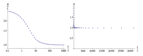
The dependence of the ratio (12) on L/λA𝐿subscript𝜆𝐴L/\lambda_{A} are seen from Fig.2 and Fig.3 in the case of ¯σ=μ+subscript¯𝜎superscript𝜇\bar{\ell}_{\sigma}=\mu^{+}. When the golden relation is applied to R.H.S of (13), R.H.S of (12) goes to 1. Thus, from the graphs in Fig.2 and Fig.3, we see that the golden relation appropriately holds for a not-so-large value of L/λA𝐿subscript𝜆𝐴L/\lambda_{A}.

Refer to caption

(a)                                                      (b)

Figure 2: R(π+(p=0),μ+;L)/L𝑅superscript𝜋𝑝0superscript𝜇𝐿𝐿R(\pi^{+}(\vec{p}=0),\mu^{+};L)/L. (a) microscopic-L𝐿L case, L/λ=0.1103𝐿𝜆0.1similar-tosuperscript103L/\lambda=0.1\sim 10^{3}, (b) intermediate-L𝐿L case, L/λ3×104𝐿𝜆3superscript104L/\lambda\leq 3\times 10^{4}. These graphs correspond to Fig.3 (a) and (b) in Ref.[3]. λπ=197.3Mev1015m139.6Mev,aμ=105.7Mev139.6Mev.formulae-sequencesubscript𝜆𝜋197.3Mevsuperscript1015m139.6Mevsubscript𝑎𝜇105.7Mev139.6Mev\lambda_{\pi}=\frac{197.3\mbox{Mev}\cdot 10^{-15}\mbox{m}}{139.6\mbox{Mev}},\;\;a_{\mu}=\frac{105.7\mbox{Mev}}{139.6\mbox{Mev}}.
Refer to caption

(a)                                                      (b)

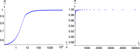
Figure 3: R(K+(p=0),μ+;L)/L,𝑅superscript𝐾𝑝0superscript𝜇𝐿𝐿R(K^{+}(\vec{p}=0),\mu^{+};L)/L, (a) L/λ3×103𝐿𝜆3superscript103L/\lambda\leq 3\times 10^{3}, (b)intermediate-L𝐿L case. Fig.3.(a) corresponds to Fig.4 in Ref.[3]. λK=197.3Mev1015m493.7Mev,aμ=105.7Mev493.7Mev.formulae-sequencesubscript𝜆𝐾197.3Mevsuperscript1015m493.7Mevsubscript𝑎𝜇105.7Mev493.7Mev\lambda_{K}=\frac{197.3\mbox{Mev}\cdot 10^{-15}\mbox{m}}{493.7\mbox{Mev}},\;\;a_{\mu}=\frac{105.7\mbox{Mev}}{493.7\mbox{Mev}}.

3 Structure of the difference (R(A+(p=0),μ+;L)L)/λA𝑅superscript𝐴𝑝0superscript𝜇𝐿𝐿subscript𝜆𝐴\bigl{(}R(A^{+}(\vec{p}=0),\mu^{+};L)-L\bigr{)}/\lambda_{A}

In this section we examine the difference (R(A+(p=0),μ+;L)L)/λA𝑅superscript𝐴𝑝0superscript𝜇𝐿𝐿subscript𝜆𝐴\bigl{(}R(A^{+}(\vec{p}=0),\mu^{+};L)-L\bigr{)}/\lambda_{A}, for λA/L<<1much-less-thansubscript𝜆𝐴𝐿1\lambda_{A}/L<<1, which gives another possible measure of the deviation from the golden relation, as mentioned in Sec.1-2. Hereafter we use for simplicity the notation R(A,μ;L)𝑅𝐴𝜇𝐿R(A,\mu;L) instead of R(A+(p=0),μ+;L)𝑅superscript𝐴𝑝0superscript𝜇𝐿R(A^{+}(\vec{p}=0),\mu^{+};L).

As to the behavior of this difference under λA/L0subscript𝜆𝐴𝐿0\lambda_{A}/L\rightarrow 0, there are three possible cases corresponding to the degree how R(A,μ;L)/L1𝑅𝐴𝜇𝐿𝐿1R(A,\mu;L)/L-1 tends to 0;

the difference =(1LR(A,μ;L)1)LλAabsent1𝐿𝑅𝐴𝜇𝐿1𝐿subscript𝜆𝐴\displaystyle=(\frac{1}{L}R(A,\mu;L)-1)\cdot\frac{L}{\lambda_{A}} (14)
λA/L0subscript𝜆𝐴𝐿0\displaystyle\overrightarrow{\lambda_{A}/L\rightarrow 0} {0if1LR(A,μ;L)1(λAL)awitha>1,const(0)if1LR(A,μ;L)1λAL,if1LR(A,μ;L)1(λAL)awith 0<a<1.cases0proportional-to𝑖𝑓1𝐿𝑅𝐴𝜇𝐿1superscriptsubscript𝜆𝐴𝐿𝑎𝑤𝑖𝑡𝑎1annotated𝑐𝑜𝑛𝑠𝑡absent0proportional-to𝑖𝑓1𝐿𝑅𝐴𝜇𝐿1subscript𝜆𝐴𝐿proportional-to𝑖𝑓1𝐿𝑅𝐴𝜇𝐿1superscriptsubscript𝜆𝐴𝐿𝑎𝑤𝑖𝑡 0𝑎1\displaystyle\begin{cases}0&if\;\frac{1}{L}R(A,\mu;L)-1\propto(\frac{\lambda_{A}}{L})^{a}\;with\;a>1,\\ const(\neq 0)&if\;\frac{1}{L}R(A,\mu;L)-1\propto\frac{\lambda_{A}}{L},\\ \infty&if\;\frac{1}{L}R(A,\mu;L)-1\propto(\frac{\lambda_{A}}{L})^{a}\;with\;0<a<1.\end{cases}

Concrete numerical calculations of R(A,μ;L)/λAL/λA𝑅𝐴𝜇𝐿subscript𝜆𝐴𝐿subscript𝜆𝐴R(A,\mu;L)/\lambda_{A}-L/\lambda_{A} for A=π+𝐴superscript𝜋A=\pi^{+} and K+superscript𝐾K^{+}, shown by Fig.4, lead to the result consistent with the middle case of (14); i.e.

1λAR(A,μ;L)LλA{1.702forA=π+,0.583forA=K+similar-to-or-equals1subscript𝜆𝐴𝑅𝐴𝜇𝐿𝐿subscript𝜆𝐴cases1.702𝑓𝑜𝑟𝐴superscript𝜋0.583𝑓𝑜𝑟𝐴superscript𝐾\frac{1}{\lambda_{A}}R(A,\mu;L)-\frac{L}{\lambda_{A}}\simeq\begin{cases}1.702&for\;A=\pi^{+},\\ -0.583&for\;A=K^{+}\end{cases} (15)

in the range 103L/λAless-than-or-similar-tosuperscript103𝐿subscript𝜆𝐴10^{3}\lesssim L/\lambda_{A} (3×10⁴)less-than-or-similar-toabsent3superscript104(\lesssim 3\times 10^{4}). It seems worthy for us to notice that the distributive law (R(A,μ;L)/L1)×LλA=R(A,μ;L)/λAL/λA𝑅𝐴𝜇𝐿𝐿1𝐿subscript𝜆𝐴𝑅𝐴𝜇𝐿subscript𝜆𝐴𝐿subscript𝜆𝐴\bigl{(}R(A,\mu;L)/L-1\bigr{)}\times\frac{L}{\lambda_{A}}=R(A,\mu;L)/\lambda_{A}-L/\lambda_{A} is confirmed numerically to hold well.

Thus we may write approximately, in the region L/λA>>1much-greater-than𝐿subscript𝜆𝐴1L/\lambda_{A}>>1,

1LR(A,μ;L)1=J1(A,μ)λAL+terms with the order (λAL)n,n2,\frac{1}{L}R(A,\mu;L)-1=J_{1}(A,\mu)\frac{\lambda_{A}}{L}+\mbox{terms with the order }\Bigl{(}\frac{\lambda_{A}}{L}\Bigl{)}^{n},\;n\geq 2, (16)

where

J1(A,μ)1.702 and J1(A,K)0.583.similar-to-or-equalssubscript𝐽1𝐴𝜇1.702 and subscript𝐽1𝐴𝐾similar-to-or-equals0.583J_{1}(A,\mu)\simeq 1.702\mbox{ and }J_{1}(A,K)\simeq-0.583. (17)

It will be neaningful to note that the deviations of the ratio R(A,μ;L)/L𝑅𝐴𝜇𝐿𝐿R(A,\mu;L)/L from 1 for not-so-large L/λA𝐿subscript𝜆𝐴L/\lambda_{A}, which are seen from Fig.2(a) and Fig.3(a), are consistent with (16) and (17), because

[CaseA=π]delimited-[]𝐶𝑎𝑠𝑒𝐴𝜋[Case\;A=\pi] Fig.2(a) leads to

1.2R(π,μ;L)L|Lλ101+J1(π,μ)10;similar-to-or-equals1.2evaluated-at𝑅𝜋𝜇𝐿𝐿similar-to-or-equals𝐿𝜆10similar-to-or-equals1subscript𝐽1𝜋𝜇101.2\simeq\frac{R(\pi,\mu;L)}{L}|_{\frac{L}{\lambda}\simeq 10}\simeq 1+\frac{J_{1}(\pi,\mu)}{10}; (18)

[CaseB=K]delimited-[]𝐶𝑎𝑠𝑒𝐵𝐾[Case\;B=K] Fig.3(a) leads to

0.95R(K,μ;L)L|Lλ101+J1(K,μ)10.similar-to-or-equals0.95evaluated-at𝑅𝐾𝜇𝐿𝐿similar-to-or-equals𝐿𝜆10similar-to-or-equals1subscript𝐽1𝐾𝜇100.95\simeq\frac{R(K,\mu;L)}{L}|_{\frac{L}{\lambda}\simeq 10}\simeq 1+\frac{J_{1}(K,\mu)}{10}. (19)
Refer to caption

(a)                                                      (b)

Figure 4: Dependence of {R(A,μ;L)L}/λA(J~(A,μ;L))annotated𝑅𝐴𝜇𝐿𝐿subscript𝜆𝐴absent~𝐽𝐴𝜇𝐿\{R(A,\mu;L)-L\}/\lambda_{A}(\equiv\tilde{J}(A,\mu;L)); (a) the case of A=π𝐴𝜋A=\pi, (b)the case of A=K𝐴𝐾A=K.

4 Additional remark on R(A,μ;L)/λAL/λA𝑅𝐴𝜇𝐿subscript𝜆𝐴𝐿subscript𝜆𝐴R(A,\mu;L)/\lambda_{A}-L/\lambda_{A}

For simplicity, we use the notation

J~(A,μ;L)=R(A,μ;L)/λAL/λA.~𝐽𝐴𝜇𝐿𝑅𝐴𝜇𝐿subscript𝜆𝐴𝐿subscript𝜆𝐴\tilde{J}(A,\mu;L)=R(A,\mu;L)/\lambda_{A}-L/\lambda_{A}. (20)

From (16), we have

J~(A,μ;L)=J1(A,μ)+ terms with the order(λAL)n1,n2.formulae-sequence~𝐽𝐴𝜇𝐿subscript𝐽1𝐴𝜇 terms with the ordersuperscriptsubscript𝜆𝐴𝐿𝑛1𝑛2\tilde{J}(A,\mu;L)=J_{1}(A,\mu)+\mbox{ terms with the order}\;\;(\frac{\lambda_{A}}{L})^{n-1},\;\;n\geq 2. (21)

With the aim of seeing why J~(A,μ;L)~𝐽𝐴𝜇𝐿\tilde{J}(A,\mu;L) has this structure, we consider the following form of J~(A,μ;L)~𝐽𝐴𝜇𝐿\tilde{J}(A,\mu;L) obtained from (12) ;

J~(A,μ;L)=(2/πaμ2(1aμ2)2I(A,μ;L)1)LλA~𝐽𝐴𝜇𝐿2𝜋subscriptsuperscript𝑎2𝜇superscript1superscriptsubscript𝑎𝜇22𝐼𝐴𝜇𝐿1𝐿subscript𝜆𝐴\tilde{J}(A,\mu;L)=\Bigl{(}\frac{2/\pi}{a^{2}_{\mu}(1-a_{\mu}^{2})^{2}}I(A,\mu;L)-1\Bigr{)}\frac{L}{\lambda_{A}} (22)

At present for convenience, we employ the notation

F(A,μ;L):=I(A,μ;L)L/λA;assign𝐹𝐴𝜇𝐿𝐼𝐴𝜇𝐿𝐿subscript𝜆𝐴F(A,\mu;L):=I(A,\mu;L)L/\lambda_{A}; (23)

then,

J~(A,μ;L)=2/πaμ2(1aμ2)2F(A,μ;L)LλA~𝐽𝐴𝜇𝐿2𝜋subscriptsuperscript𝑎2𝜇superscript1superscriptsubscript𝑎𝜇22𝐹𝐴𝜇𝐿𝐿subscript𝜆𝐴\tilde{J}(A,\mu;L)=\frac{2/\pi}{a^{2}_{\mu}(1-a_{\mu}^{2})^{2}}F(A,\mu;L)-\frac{L}{\lambda_{A}} (24)

By using the concrete form of I(A,μ;L)𝐼𝐴𝜇𝐿I(A,\mu;L), i.e.formulae-sequence𝑖𝑒i.e. Eq. (13), we have

dF(A,μ;L)dL𝑑𝐹𝐴𝜇𝐿𝑑𝐿\displaystyle\frac{dF(A,\mu;L)}{dL} =\displaystyle= 2λA0𝑑bb2(1baσ2+b2)2subscript𝜆𝐴superscriptsubscript0differential-d𝑏superscript𝑏21𝑏superscriptsubscript𝑎𝜎2superscript𝑏2\displaystyle\frac{2}{\lambda_{A}}\int_{0}^{\infty}db\cdot b^{2}\bigl{(}1-\frac{b}{\sqrt{a_{\sigma}^{2}+b^{2}}}\bigr{)} (25)
×\displaystyle\times sin(L2λA(1aσ2+b2b)cos(L2λA(1aσ2+b2b))(1aσ2+b2b)/2;\displaystyle\frac{\sin\bigl{(}\frac{L}{2\lambda_{A}}(1-\sqrt{a_{\sigma}^{2}+b^{2}}-b)\cos\bigl{(}\frac{L}{2\lambda_{A}}(1-\sqrt{a_{\sigma}^{2}+b^{2}}-b)\bigr{)}}{(1-\sqrt{a_{\sigma}^{2}+b^{2}}-b)/2};

therefore,

λAdJ~(A,μ;L)dL=2/πaμ2(1aμ2)2λAdF(A,μ;L)dL1subscript𝜆𝐴𝑑~𝐽𝐴𝜇𝐿𝑑𝐿2𝜋subscriptsuperscript𝑎2𝜇superscript1superscriptsubscript𝑎𝜇22subscript𝜆𝐴𝑑𝐹𝐴𝜇𝐿𝑑𝐿1\lambda_{A}\frac{d\tilde{J}(A,\mu;L)}{dL}=\frac{2/\pi}{a^{2}_{\mu}(1-a_{\mu}^{2})^{2}}\cdot\lambda_{A}\frac{dF(A,\mu;L)}{dL}-1 (26)

with

λAdF(A,μ;L)dL=0𝑑bb2(1baσ2+b2)2sin(LλA(1aσ2+b2b)1aσ2+b2b.\lambda_{A}\frac{dF(A,\mu;L)}{dL}=\int_{0}^{\infty}db\cdot b^{2}\bigl{(}1-\frac{b}{\sqrt{a_{\sigma}^{2}+b^{2}}}\bigr{)}\frac{2\sin\bigl{(}\frac{L}{\lambda_{A}}(1-\sqrt{a_{\sigma}^{2}+b^{2}}-b)}{1-\sqrt{a_{\sigma}^{2}+b^{2}}-b}. (27)

From Eq. (16) and Fig.4, J~(A,μ;L)~𝐽𝐴𝜇𝐿\tilde{J}(A,\mu;L) is seen to be nearly L𝐿L-independent and

J~(A,μ;L)J1(A,μ) for 103L/λA.similar-to-or-equals~𝐽𝐴𝜇𝐿subscript𝐽1𝐴𝜇 for superscript103less-than-or-similar-to𝐿subscript𝜆𝐴\tilde{J}(A,\mu;L)\simeq J_{1}(A,\mu)\mbox{ for }10^{3}\lesssim L/\lambda_{A}. (28)

The consistence of our calculation is seen, through numerical evaluation of the integral (27), by confirming

|R.H.S.of(26)|1.|R.H.S.\;of\;(\ref{eq:1.27})|\ll 1. (29)

It seems meaningful to note the Dirac delta function is expressed as

δ(x)=limgsin(gx)πx.𝛿𝑥subscript𝑔𝑔𝑥𝜋𝑥\delta(x)=\lim_{g\rightarrow\infty}\frac{\sin(gx)}{\pi x}. (30)

(See Ref.[5].) By applying this relation to R.H.S. of Eq. (27), we obtain, as expected,

λAdF(A,μ;L)dLlargeL/λAπ2aμ2(1aμ2)2.𝑙𝑎𝑟𝑔𝑒𝐿subscript𝜆𝐴subscript𝜆𝐴𝑑𝐹𝐴𝜇𝐿𝑑𝐿𝜋2subscriptsuperscript𝑎2𝜇superscript1subscriptsuperscript𝑎2𝜇2\lambda_{A}\frac{dF(A,\mu;L)}{dL}\;\xrightarrow{large\;L/\lambda_{A}}\frac{\pi}{2}a^{2}_{\mu}(1-a^{2}_{\mu})^{2}. (31)

This shows the numerical calculations leading to (29) have been correctly performed.

In the considerations described in this report, we have investigated the structures of the ratio R(A(p),μ;L)/L𝑅𝐴𝑝𝜇𝐿𝐿R(A(\vec{p}),\mu;L)/L and the difference (R(A(p),μ;L)L)/λA𝑅𝐴𝑝𝜇𝐿𝐿subscript𝜆𝐴\bigl{(}R(A(\vec{p}),\mu;L)-L\bigr{)}/\lambda_{A} in the case of p=0𝑝0\vec{p}=0 for simplicity. These quantities have characteristic features related with the deviation from Fermi’s golden relation. We hope those features are confirmed experimentally.

References

  • [1] K.Fujii and T.Shimomura, Prog.Theor. Phys. 112,901(2004);arXiv:hep-ph/0406079[Search in SPIRE].
  • [2] K.Fujii and T.Shimomura, Phys. of Atomic Nuclei 69(2006),1353(2006).
  • [3] K.Fujii and N. Toyota, Prog. Theor. Exp. Phys., 2015, 023301. DOI:10.1093/ptep/ptu178.
  • [4] K.Ishikawa and Y. Tobita, Prog.Theor. Exp. Phys. 2013, 073B02(2013).
  • [5] E.g. L.Schiff, ”Quantum Mechanics”, MaGRAW-Hill, NewYork, 1955