Multidimensional lower density versions of Plünnecke’s inequality

Abstract.

We investigate the lower asymptotic density of sumsets in $\mathbb{N}^{2}$ by proving certain Plünnecke type inequalities for various notions of lower density in $\mathbb{N}^{2}$. More specifically, we introduce a notion of lower tableaux density in $\mathbb{N}^{2}$ which involves averaging over convex tableaux-shaped regions in $\mathbb{N}^{2}$ which contain the origin. This generalizes the well known Plünnecke type inequality for the lower asymptotic density of sumsets in $\mathbb{N}$. We also provide a conjectural Plünnecke inequality for the more basic notion of lower rectangular asymtpotic density in $\mathbb{N}^{2}$ and prove certain partial results.

1. Introduction

1.1. Background

Plünnecke’s classical work [6] provided influential techniques for studying the cardinality of sumsets and iterated sumsets. We recall that for subsets $A,B$ of an abelian group $(G,+)$ we can define the sumset

$$A+B=\{a+b\text{ }|\text{ }a\in A,b\in B\}$$

and, for positive integers $k$, the $k$-fold iterated sumset

$$kA=\{a_{1}+\cdots+a_{k}\text{ }|\text{ }a_{1},\ldots,a_{k}\in A\}.$$

Theorem 1.1 (Plünnecke [6]).

Suppose that $A,B$ are finite subsets of some abelian group $(G,+)$ and $k\geq 1$. Then

$$|A+B|\geq|A|^{1-\frac{1}{k}}|kB|^{1/k}.$$

Plünnecke used these techniques to improve a result of Erdős concerning lower bounds for the Schnirelmann density of a sumset $A+B$, where $A,B\subset\mathbb{Z}_{\geq 0}$ and $B$ is a basis of order $k$ (that is, $kB=\mathbb{N}=\{0,1,2,\ldots\}$). We define the Schnirelmann density of a subset $A\subset\mathbb{N}=\{0,1,\ldots\}$ to be

(1.1) $$\sigma(A)=\inf_{n\in\mathbb{N}}\frac{|A\cap[0,n]|}{n+1}.$$

Note that the usual definition is $\sigma(A)=\inf_{n\geq 1}\frac{|A\cap[1,n]|}{n}$, which is necessary for some applications such as Mann’s Theorem, but the results of interest to us remain valid when using our definition. Erdös proved that

$$\sigma(A+B)\geq\left(1+\frac{1-\sigma(A)}{2k}\right)\sigma(A)$$

for $A,B\subset\mathbb{N}$ such that $kB=\mathbb{N}$ for some positive integer $k$ [3]. Plünnecke greatly improved this lower bound by proving the following extension of his cardinality estimate (Theorem 1.1) to Schnirelmann density.

Theorem 1.2 (Plünnecke’s inequality for Schnirelmann density [6]).

For positive integers $k$ and $A,B\subset\mathbb{N}$ with $0\in B$, we have that

$$\sigma(A+B)\geq\sigma(A)^{1-\frac{1}{k}}\sigma(kB)^{1/k}.$$

A good account of this as well as a proof of Theorem 1.1 and related results can be found in Ruzsa’s book [7]. Although Schnirelmann density has played an important role in additive number theory (see, for instance, Schnirelmann’s proof that the primes are an asymptotic basis [8]), it lacks many asymptotic features such as translation invariance. From a combinatorial perspective, the lower asymptotic density, given by

$$\underline{d}(A)=\liminf_{n\to\infty}\frac{|A\cap[0,n]|}{n+1},$$

is a more natural notion of the asymptotic size of a set $A\subset\mathbb{N}$. It turns out that Theorem 1.2 is also true with $\underline{d}$ in place of $\sigma$.

Theorem 1.3 (See [4], [5] and [7]).

Suppose that $A,B\subset\mathbb{N}$ and $k\geq 1$. Then

$$\underline{d}(A+B)\geq\underline{d}(A)^{1-\frac{1}{k}}\underline{d}(kB)^{1/k}.$$

This was first obtained by Ruzsa [7] and an alternative proof, which the author has found insightful, was given by Jin in [4] and [5].

1.2. Density Plünnecke inequalites in (semi)groups

It is natural to ask whether density versions of Plünnecke’s inequality hold in other countable abelian (semi)groups with certain notions of asymptotic density. Let us briefly mention some recently established results in this direction. We first recall a standard way of extending the notion of density to other groups that involves replacing the sequence of intervals $\left([0,N)\cap\mathbb{Z}\right)_{N=1}^{\infty}$ with a sequence of asymptotically invariant finite sets.

Definition 1.4 (Densities along Følner sequences).

Let $(G,+)$ be a countable abelian semigroup. A Følner sequence is a sequence $F_{1},F_{2},\ldots$ of finite subsets of $G$ that is asymptotically invariant, i.e., for each $g\in G$ we have that

$$\lim_{n\to\infty}\frac{|F_{n}\cap(g+F_{n})|}{|F_{n}|}=1.$$

Moreover, if $A\subset G$ then we define the lower asymptotic density along $(F_{n})$ as

$$\underline{d}_{(F_{n})}(A)=\liminf_{n\to\infty}\frac{|F_{n}\cap A|}{|F_{n}|}.$$

Similairly, we may define the upper asymptotic density along $(F_{n})$ as

$$\overline{d}_{(F_{n})}(A)=\limsup_{n\to\infty}\frac{|F_{n}\cap A|}{|F_{n}|}.$$

If $\mathcal{F}$ is a collection of Følner sequences in $G$ then we can define the lower and upper densities with respect to this collection as

$$\underline{d}_{\mathcal{F}}(A)=\inf\left\{\underline{d}_{(F_{n})}(A)\text{ }|\text{ }(F_{n})\in\mathcal{F}\right\}$$

and

$$\overline{d}_{\mathcal{F}}(A)=\sup\left\{\overline{d}_{(F_{n})}(A)\text{ }|\text{ }(F_{n})\in\mathcal{F}\right\}.$$

Finally, the lower and upper Banach densities in $G$ may be defined, respectively, as

$$d_{\ast}=\underline{d}_{\textbf{F{\o}lner}(G)}\text{ and }d^{\ast}=\overline{d}_{\textbf{F{\o}lner}(G)}$$

where $\textbf{F{\o}lner}(G)$ denotes the collection of all Følner sequences in $G$.

Theorem 1.5 ([2]; $k^{\prime}=1$ case obtained in [1]).

Suppose that $(G,+)$ is a countable abelian group and $A,B\subset G$. Then for integers $0<k^{\prime}<k$ we have

$$d^{*}(A+k^{\prime}B)\geq d^{*}(kB)^{\frac{k^{\prime}}{k}}d^{*}(A)^{1-\frac{k^{\prime}}{k}}$$

and

$$d_{*}(A+k^{\prime}B)\geq d^{*}(kB)^{\frac{k^{\prime}}{k}}d_{*}(A)^{1-\frac{k^{\prime}}{k}}.$$

For the semigroup $G=\mathbb{N}$, the $k^{\prime}=1$ cases of these inequalities were obtained by Jin in [5]. We remark that the proofs of Theorem 1.5 (for arbitrary countable abelian groups $G$) use ergodic theory and it is unclear whether such techniques can be applied to densities associated to smaller classes of Følner sequences, such as lower asymptotic density. The purpose of this paper is to extend the Plünnecke type inequality for lower asymptotic density to the semigroup $\mathbb{N}^{2}$.

1.3. Følner sequences and lower asymptotic density in $\mathbb{N}^{2}$

A natural candidate for lower asymptotic density in $\mathbb{N}^{2}$ arises from considering the family

$$\textbf{Rect}=\left\{\left([0,W_{k}]\times[0,H_{k}]\cap\mathbb{N}^{2}\right)_{k=1}^{\infty}\text{ }|\text{ }W_{k},H_{k}\to\infty\text{ as }k\to\infty\right\}\subset\textbf{F{\o}lner}(\mathbb{N}^{2}),$$

as the corresponding lower density is a product density in the sense that

$$\underline{d}_{\textbf{Rect}}(A\times B)=\underline{d}(A)\underline{d}(B),$$

for $A,B\subset\mathbb{N}^{2}$. In the one-dimensional case, the collection $\{[0,W_{k}]\cap\mathbb{N}^{2}\text{ }|\text{ }W_{k}\to\infty\text{ as }k\to\infty\}$ of sequences of intervals which gives rise to the lower density $\underline{d}$ in $\mathbb{N}$ satisfies the desirable property of being closed under pointwise unions. Unfortunately, Rect does not satisfy this property, so it seems natural to consider

(1.2) $$\textbf{Tab}=\bigcup_{L=1}^{\infty}\left\{\left(R^{(1)}_{k}\cup R^{(2)}_{k}\cup\ldots\cup R^{(L)}_{k}\right)_{k=1}^{\infty}\text{ }|\text{ }\left(R^{(i)}_{k}\right)_{k=1}^{\infty}\in\textbf{Rect}\text{ for }i=1,2\ldots,L\right\},$$

which is the smallest subset of $\textbf{F{\o}lner}(G)$ that contains Rect and is closed under pointwise unions. The corresponding lower density $\underline{d}_{\textbf{Tab}}$ has the curious property that it is also a product density as above and hence agrees with $\underline{d}_{\textbf{Rect}}$ on cartesian products, i.e.,

$$\underline{d}_{\textbf{Tab}}(A\times B)=\underline{d}(A)\underline{d}(B)=\underline{d}_{\textbf{Rect}}(A\times B),$$

for $A,B\subset\mathbb{N}$ (See Appendix B). In fact, this property is also satisfied by the collection

$$\textbf{Tab}(L)=\left\{\left(R^{(1)}_{k}\cup R^{(2)}_{k}\cup\ldots\cup R^{(L)}_{k}\right)_{k=1}^{\infty}\text{ }|\text{ }\left(R^{(i)}_{k}\right)_{k=1}^{\infty}\in\textbf{Rect}\text{ for }i=1,2\ldots,L\right\}$$

for all $L\in\mathbb{N}$, which is itself a family of Følner sequences that we will be interested in.

1.4. Lower density versions of Plünnecke’s inequality in $\mathbb{N}^{2}$

The main goal of this paper is to address the following question.

Question 1.6.

For $A,B\subset\mathbb{N}^{2}$, with $(0,0)\in B$, and positive integers $k^{\prime}<k$, is it true that

$$\underline{d}_{\textbf{Rect}}(A+k^{\prime}B)\geq\underline{d}_{\textbf{Rect}}(A)^{1-\frac{k^{\prime}}{k}}\underline{d}_{\textbf{Rect}}(kB)^{\frac{k^{\prime}}{k}}?$$

Our first partial result is an affirmative answer to this question when $A\subset\mathbb{N}^{2}$ is such that the density $d_{\textbf{Rect}}(A)$ exists, by which we mean that

$$\underline{d}_{\textbf{Rect}}(A)=\overline{d}_{\textbf{Rect}}(A).$$

In this case, we denote this common value by $d_{\textbf{Rect}}(A)$.

Proposition 1.7 (Plünnecke inequalities for $\underline{d}_{\textbf{Rect}}$ when density of $A$ exists).

Suppose that $A\subset\mathbb{N}^{2}$ is such that $d_{\textbf{Rect}}(A)$ exists. Then for all $B\subset\mathbb{N}^{2}$ with $(0,0)\in B$ and integers $0<k^{\prime}<k$ we have that

$$\underline{d}_{\textbf{Rect}}(A+k^{\prime}B)\geq d_{\textbf{Rect}}(A)^{1-\frac{k^{\prime}}{k}}\underline{d}_{\textbf{Rect}}(kB)^{\frac{k^{\prime}}{k}}.$$

Remark 1.8.

Note that it is very easy to affirmatively answer Question 1.6 up to a constant by using the fact that $(A\cap[0,N]\times[0,M])+(B\cap[0,N]\times[0,M])\subset(A+B)\cap[0,2N]\times[0,2M]$. For instance, one may use this fact to immediately deduce that for $A,B\subset\mathbb{N}^{2}$ and positive integers $k$, we have that

$$\underline{d}_{\textbf{Rect}}(A+B)\geq\frac{1}{4}\underline{d}_{\textbf{Rect}}(A)^{1-\frac{1}{k}}\underline{d}_{\textbf{Rect}}(kB)^{\frac{1}{k}}.$$

The constant becomes much worse than $\frac{1}{4}$ if one applies this method to estimate the lower densities of $A+k^{\prime}B$ for $k^{\prime}<k$ large; more precisely, one gets

$$\underline{d}_{\textbf{Rect}}(A+k^{\prime}B)\geq\frac{1}{(1+k^{\prime})^{2}}\underline{d}_{\textbf{Rect}}(A)^{1-\frac{k^{\prime}}{k}}\underline{d}_{\textbf{Rect}}(kB)^{\frac{k^{\prime}}{k}}.$$

1.5. Statements of main results and applications

We are able to affirmatively answer Question 1.6 if we replace Rect with the collection Tab introduced above in (1.2). An element of Tab will be refered to as a tableau Følner sequence and we will refer to the corresponding notion of lower density $\underline{d}_{\textbf{Tab}}$ (as per Definition 1.4) as the lower tableau density.

Theorem 1.9.

Let $A,B\subset\mathbb{N}^{2}$ such that $(0,0)\in B$. Then

$$\underline{d}_{\textbf{Tab}}(A+k^{\prime}B)\geq\underline{d}_{\textbf{Tab}}(A)^{1-k^{\prime}/k}\underline{d}_{\textbf{Tab}}(kB)^{k^{\prime}/k}$$

for integers $0<k^{\prime}<k$.

In fact, our techniques also give the following partial answer to Question 1.6.

Theorem 1.10.

Suppose that $0<k^{\prime}<k$ are integers and $A,B\subset\mathbb{N}^{2}$ such that $(0,0)\in B$, then

$$\underline{d}_{\textbf{Rect}}(A+k^{\prime}B)\geq\underline{d}_{\textbf{Tab}}(A)^{1-\frac{k^{\prime}}{k}}\underline{d}_{\textbf{Rect}}(kB)^{\frac{k^{\prime}}{k}}.$$

This enables us to affirmatively answer Question 1.6 for a broader class of examples not covered by Proposition 1.7.

Corollary 1.11.

Suppose that $0<k^{\prime}<k$ are integers and $A,B\subset\mathbb{N}^{2}$ such that $(0,0)\in B$, $\underline{d}_{\textbf{Tab}}(A)=\underline{d}_{\textbf{Rect}}(A)$. Then

$$\underline{d}_{\textbf{Rect}}(A+k^{\prime}B)\geq\underline{d}_{\textbf{Rect}}(A)^{1-\frac{k^{\prime}}{k}}\underline{d}_{\textbf{Rect}}(kB)^{\frac{k^{\prime}}{k}}.$$

In particular, since $\underline{d}_{\textbf{Tab}}(A)=d_{\textbf{Rect}}(A)$ whenever $d_{\textbf{Rect}(A)}$ exists, we get Proposition 1.7. Theorems 1.9 and 1.10 are both immediate consequences of the following general result.

Theorem 1.12.

Suppose that $0<k^{\prime}<k$ are integers and $A,B\subset\mathbb{N}^{2}$ such that $(0,0)\in B$, then

$$\underline{d}_{\textbf{Tab}(L)}(A+k^{\prime}B)\geq\underline{d}_{\textbf{Tab}}(A)^{1-\frac{k^{\prime}}{k}}\underline{d}_{\textbf{Tab}(L)}(kB)^{\frac{k^{\prime}}{k}}$$

for all $L\in\mathbb{N}$.

1.6. Examples: Fractal Sets

We now turn to constructing some examples of subsets of $\mathbb{N}^{2}$ which demonstrate the novelty of our main result and its corollary. We are able to give lower bounds for $\underline{d}_{\textbf{Rect}}(A+k^{\prime}B)$ in the case where $A$ possesses a certain fractal structure and $B$ is a rectangular asymptotic basis of order $k>k^{\prime}$ (that is, $\underline{d}_{\textbf{Rect}}(kB)=1$). We give an example of such a fractal set before giving a broad definition.

Example 1.13 (A fractal set and an application of Theorem 1.9).

In this example, by $[a,b)$ we mean $\{x\in\mathbb{N}|a\leq x<b\}$ for $a<b\in\mathbb{N}$. Choose a sequence $0<u_{1}<u_{2}<\ldots$ in $\mathbb{N}^{2}$ such that $u_{k}>2u_{k-1}$ for $k>1$ and $\lim_{k\to\infty}\frac{u_{k}}{u_{k-1}}=\infty$. Let $A\subset\mathbb{N}$ be the set given in Figure 1, more precisely

$$A=[0,u_{1})^{2}\cup[u_{1},2u_{1})^{2}\cup\bigcup_{k=2}^{\infty}[u_{k},2u_{k})^{2}\cup\left([0,u_{k})^{2}\setminus[0,2u_{k-1})^{2}\right).$$

Figure 1. The set $A$ in Example 1.13.

One sees that $\underline{d}_{\textbf{Rect}}(A)=\frac{1}{2}$ and $\overline{d}_{\textbf{Rect}}(A)=1$ (for details, see Proposition1.15). However one may still give a lower bound for $\underline{d}_{\textbf{Rect}}(A+B)$ (which is greater than the trivial lower bound $\underline{d}_{\textbf{Rec}}(A)$) for arbitrary $B\subset\mathbb{N}^{2}$ such that $B+B=\mathbb{N}^{2}$, as follows. It is not hard to see (Proposition 1.15) that $\underline{d}_{\textbf{Tab}}(A)=\frac{1}{3}$. Thus by Theorem 1.9 we have that

$$\underline{d}_{\textbf{Rect}}(A+B)\geq\underline{d}_{\textbf{Tab}}(A+B)\geq\underline{d}_{\textbf{Tab}}(A)^{1/2}\underline{d}_{\textbf{Tab}}(B+B)^{1/2}=\frac{1}{\sqrt{3}}.$$

One can generalise the example above to construct more general sets that are asymptotically finite unions of translates of a large square.

Definition 1.14 (Fractal set generated by a pattern).

As before, we will use the convention $[a,b)=\{x\in\mathbb{N}\text{ }|\text{ }a\leq x<b\}$. Let $N\in\mathbb{N}$ and

$$P\subset\{0,1,\ldots,N\}\times\{0,1,\ldots,N\}$$

be a set such that $(0,0)\in P$. We call such a $P$ a pattern. Choose a sequence $u_{1},u_{2},\ldots$ of positive integers such that $u_{k}>(N+1)u_{k-1}$ and $\lim_{k\to\infty}\frac{u_{k}}{u_{k-1}}=\infty$. Define

$$\mathcal{P}_{k}=\{u_{k}p\text{ }|\text{ }p\in P\}+[0,u_{k})^{2}$$

and let

$$A_{k}=\mathcal{P}_{k}\setminus[0,(N+1)u_{k-1})^{2}$$

where $u_{0}=0$ (in other words $A_{1}=\mathcal{P}_{1}$). Finally, we define $A(P,N)=\bigcup_{k=1}^{\infty}A_{k}$ to be the fractal set generated by the pattern $P$ of degree $N$.

Figure 2. Definition 1.14 for the case $N=2$, $P=\{(0,0),(0,2),(2,2)\}$. Note that $A_{k}$ is contained in $[0,3u_{k})^{2}\setminus[0,3u_{k-1})^{2}$; while $\mathcal{P}_{j}$ and $A_{j}$ are contained in the small square $[0,3u_{k-1})^{2}$, for all $j<k$.

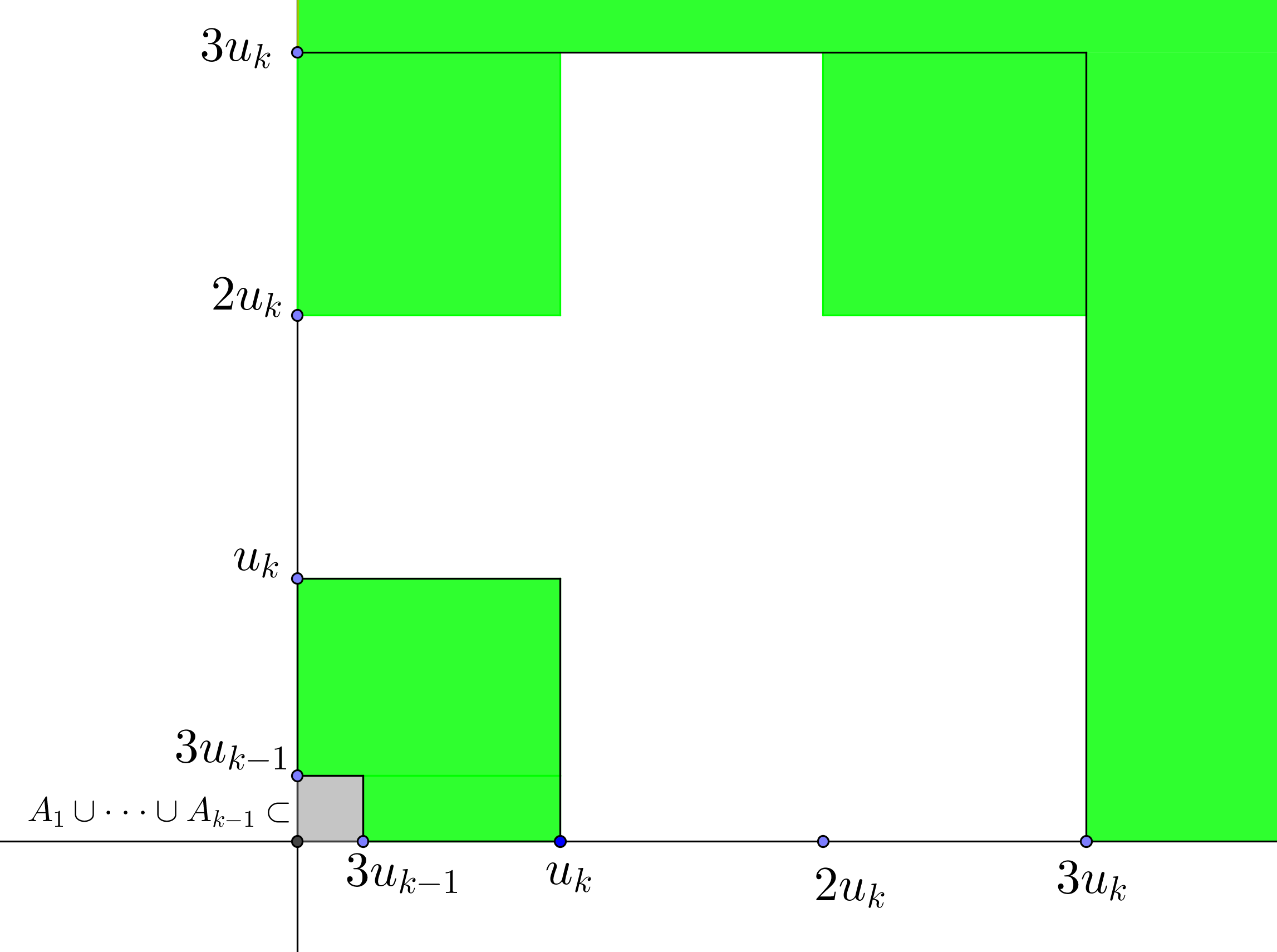
Note that the set $A$ given in Example 1.13 is $A(P,1)$ for $P=\{(0,0),(1,1)\}$. We now give a combinatorial formula for $\underline{d}_{\textbf{Tab}}$ and $\underline{d}_{\textbf{Rect}}$ of fractal sets generated by a pattern.

Proposition 1.15.

Suppose that $N\in\mathbb{N}$ and $P\subset\{0,1,\ldots,N\}\times\{0,1,\ldots,N\}$ and let $A=A(P,N)$. Then

$$\underline{d}_{\textbf{Rect}}(A)=\min\left\{\frac{|P\cap I|}{|I|}\text{ }|\text{ }I=[0,m]\times[0,n]\cap\mathbb{N}^{2}\text{ for some }m,n\in\{0,1,\ldots,N\}\right\}$$

and

$$\underline{d}_{\textbf{Tab}}{A}=\min\left\{\frac{|P\cap T|}{|T|}\text{ }|\text{ }T\subset\{0,\ldots,N\}\times\{0,\ldots,M\}\text{ is a tableau.}\right\}$$

where we define a tableau to be a set of the form

$$\bigcup_{(n,m)\in F}\{0,1,\ldots,n\}\times\{0,1,\ldots,m\}$$

for some finite $F\subset\mathbb{N}^{2}$.

Proof: See Appendix A. $\blacksquare$

Thus $\underline{d}_{\textbf{Rect}}(A)<1=\overline{d}_{\textbf{Rect}}(A)$ for all fractal sets other than $\mathbb{N}^{2}$, which leads to many applications of our results that do not follow from Proposition 1.7.

Example 1.16.

Let $P=\{(0,0),(0,2),(2,2)\}$ and let $A=A(P,2)$ (as depicted in Figure 2). Then

$$\underline{d}_{\textbf{Rect}}(A)=\underline{d}_{\textbf{Tab}}(A)=\frac{1}{6}.$$

Thus if $(0,0)\in B\subset\mathbb{N}^{2}$ and $k>0$ is an integer then by Theorem 1.10 we have

$$\underline{d}_{\textbf{Rect}}(A+k^{\prime}B)\geq\underline{d}_{\textbf{Rect}}(A)^{1-\frac{k^{\prime}}{k}}\underline{d}_{\textbf{Rect}}(kB)^{\frac{k^{\prime}}{k}}$$

for integers $0<k^{\prime}<k$. Many such special cases of Question 1.6 may be constructed, which are not covered by Proposition 1.7.

1.7. A remark about higher dimensions

When $B$ is an asymptotic basis of order $k$ (i.e., $kB=\mathbb{N}^{2}$), the natural analogue of Theorem 1.12 (and hence also its consequences) holds in higher dimensions, as the reader may observe in the equation (6.13) found in the proof of Theorem 1.12 in Section 6. However, it is yet unclear whether the higher dimensional analogue of Theorem 1.12 holds in full generality, the main obstacle lies in finding the right higher dimensional extension of Lemma 5.7.

1.8. Organization of the paper

In Section 2 we review some classical Plünnecke inequalities for cardinalities of truncated sumsets (i.e., sets of the form $(A+B)\setminus C$), as well as the less well known but crucial $\delta$-heavy Plünnecke inequality. In Section 3 we introduce the main definitions, notations and conventions. In particular, we introduce the notion of a tableau, the main combinatorial object in this paper, and we establish some basic properties of the lower tableau density $\underline{d}_{\textbf{Tab}}$. Sections 4 and 5 include some technical combinatorial lemmata involving tableaux that will be put together in Section 6 to conclude the proof of Theorem 1.12. In Section 7 we state some related open problems; more specifically, some conjectural multidimensional Plünnecke inequalities for various densities. Finally, Appendix A is devoted to proving Proposition 1.15.

Acknowledgement: The author is grateful for many insightful and encouraging conversations with Alexander Fish.

2. Plünnecke inequalities for truncated sumsets

One of the key tools used in the proof of our results, as well as Jin’s proofs in [4] and [5], is the following Plünnecke inequality for truncated sumsets.

Theorem 2.1 (See [7]).

Let $A,B,C$ be finite subsets of an abelian group and define

$$D_{n}=D_{n}(A,B,C)=\min_{\emptyset\neq A^{\prime}\subset A}\frac{|(A^{\prime}+nB)\setminus(C+(n-1)B)|}{|A^{\prime}|}.$$

Then $D^{1/n}_{n}$ is decreasing in $n$.

We will need (unlike Jin in [4] and [5]) the following $\delta$-heavy version of this inequality. We will include a proof for the sake of completeness as this version, to the best of the author’s knowledge, rarely appears in the literature (cf. [1]).

Theorem 2.2.

Let $A,B,C$ be finite subsets of an abelian group and let $0<\delta<1$. Then for positive integers $k^{\prime}<k$, there exists $A^{\prime}\subset A$ such that $|A^{\prime}|>\delta|A|$ and

$$\frac{|(A^{\prime}+kB)\setminus(C+(k-1)B)|}{|A^{\prime}|}\leq(1-\delta)^{-k/k^{\prime}}\left(\frac{|(A+k^{\prime}B)\setminus(C+(k^{\prime}-1)B)|}{|A|}\right)^{k/k^{\prime}}.$$

Proof: Using Theorem 2.1 and the fact that $(1-\delta)^{-k/k^{\prime}}>1$, take non-empty $A^{\prime}\subset A$ of maximal cardinality such that

(2.1) $$|(A^{\prime}+kB)\setminus(C+(k-1)B)|\leq(1-\delta)^{-k/k^{\prime}}\left(\frac{|(A+k^{\prime}B)\setminus(C+(k^{\prime}-1)B)|}{|A|}\right)^{k/k^{\prime}}|A^{\prime}|.$$

Suppose for contradiction that $|A^{\prime}|\leq\delta|A|$, thus $|A\setminus A^{\prime}|\geq(1-\delta)|A|$. Now apply Theorem 2.1, with $A\setminus A^{\prime}$ playing the role of $A$, to obtain a non-empty $A^{\prime\prime}\subset A\setminus A^{\prime}$ such that

$$|(A^{\prime\prime}+kB)\setminus(C+(k-1)B)|\leq\left(\frac{|((A\setminus A^{\prime})+k^{\prime}B)\setminus(C+(k^{\prime}-1)B)|}{|A\setminus A^{\prime}|}\right)^{k/k^{\prime}}|A^{\prime\prime}|.$$

We deduce from this inequality, using the fact that $A\setminus A^{\prime}\subset A$ and $|A\setminus A^{\prime}|\geq(1-\delta)|A|$, the estimate

(2.2) $$|(A^{\prime\prime}+kB)\setminus(C+(k-1)B)|\leq(1-\delta)^{-k/k^{\prime}}\left(\frac{|(A+k^{\prime}B)\setminus(C+(k^{\prime}-1)B)|}{|A|}\right)^{k/k^{\prime}}|A^{\prime\prime}|.$$

Now by adding the estimates (2.1) and (2.2) we get

$$|((A^{\prime}\cup A^{\prime\prime})+kB)\setminus(C+(k-1)B)|\leq(1-\delta)^{-k/k^{\prime}}\left(\frac{|(A+k^{\prime}B)\setminus(C+(k^{\prime}-1)B)|}{|A|}\right)^{k/k^{\prime}}|A^{\prime}\cup A^{\prime\prime}|.$$

But since $A^{\prime\prime}$ is non-empty, this contradicts the maximality of $A^{\prime}$. $\blacksquare$

3. Tableaux

We stress that throughout this paper we use (and already have used) the convention $\mathbb{N}=\{0,1,\ldots\}$. A tableau is a set of the form

$$\bigcup_{(N,M)\in F}\{0,1,\ldots,N\}\times\{0,1,\ldots M\}$$

where $F\subset\mathbb{N}^{2}$ is a finite set. It will also be convenient to define a tableau region to be a set of the form

$$\bigcup_{(N,M)\in F}[0,N)\times[0,M)$$

for some finite $F\subset\mathbb{N}^{2}$. Thus a tableau is precisely the set of lattice points of some tableau region.

Important note on notation: If $A$ is a union of rectangles of the form $[N,N+1)\times[M,M+1)$ where $N,M\in\mathbb{Z}$ (such as a tableau region), then by $|A|$ we mean the Lebesgue measure of $A$, which is also the number of integer points in $A$. For most of our arguments, it is more conceptual to consider the more geometric and continuous notion of Lebesgue measure. Unless otherwise specified, by $[a,b)$ we mean $\{x\in\mathbb{R}\text{ }|\text{ }a\leq x<b\}$ (very rarely it will mean $\{x\in\mathbb{Z}\text{ }|\text{ }a\leq x<b\}$, in fact only in the definition of fractal sets in the Introduction above and Appendix A).

We note the following simple but useful additive characterization of tableaux.

Lemma 3.1.

If $T\subset\mathbb{N}^{2}$ is finite and non-empty, then the following are equivalent:

1. $T$ is a tableau.

2. $\mathbb{N}^{2}\setminus T$ is invariant under addition by elements of $\mathbb{N}^{2}$, i.e., $(\mathbb{N}^{2}\setminus T)+a\subset\mathbb{N}^{2}\setminus T$ for all $a\in\mathbb{N}^{2}$.

This means that if $T$ is a tableau and $B\subset\mathbb{N}^{2}$ contains $(0,0)$, then $(\mathbb{N}^{2}\setminus T)+B=\mathbb{N}^{2}\setminus T$. As a consequence, we may apply Theorem 2.2 with $C=\mathbb{N}^{2}\setminus T$ to obtain the following crucial proposition.

Proposition 3.2.

Let $T\subset\mathbb{N}$ be a tableau and suppose that $A,B\subset\mathbb{N}^{2}$ with $(0,0)\in B$. Then for positive integers $k^{\prime}<k$ and $0<\delta<1$, there exists $A^{\prime}\subset A$ such that $|A^{\prime}|>\delta|A|$ and

$$\frac{|(A^{\prime}+kB)\cap T|}{|A^{\prime}|}\leq(1-\delta)^{-k/k^{\prime}}\left(\frac{|(A+k^{\prime}B)\cap T|}{|A|}\right)^{k/k^{\prime}}.$$

We now turn to explicating some basic properties of the densities $\underline{d}_{\textbf{Tab}}$ and $\underline{d}_{\textbf{Tab}(L)}$ that were introduced above. The following simple lemma will be convenient as it shows that we may, without loss of generality, assume that the side lengths of our rectangles are divisible by a chosen integer.

Lemma 3.3.

Let $D,L$ be positive integers and $A\subset\mathbb{N}^{2}$. Then there exists a sequence of the form

$$F_{n}=\bigcup_{j=1}^{\ell(n)}[0,W_{j,n})\times[0,H_{j,n})$$

with each $\ell(n)\leq L$, such that

1. For each $j\in\{1,\ldots,\ell(n)\}$, we have

   $$W_{j,n}\equiv H_{j,n}\equiv 0\mod D.$$

2. The $W_{i,n}$ and $H_{i,n}$ tend to $\infty$, more precisely

   $$\lim_{n\to\infty}\min_{i\in\{1,\ldots,\ell(n)\}}W_{i,n}=\lim_{n\to\infty}\min_{i\in\{1,\ldots,\ell(n)\}}H_{i,n}=\infty.$$

3. $$\liminf_{n\to\infty}\frac{|A\cap F_{n}|}{|F_{n}|}=\underline{d}_{\textbf{Tab}(L)}(A).$$

Proof Sketch: The idea is that if one replaces $W_{i,n}$ with $W_{i,n}+O(1)$ then

$$\liminf_{n\to\infty}\frac{|A\cap F_{n}|}{|F_{n}|}$$

remains unchanged. Applying this finitely many times, we can adjust a sequence satisfying (iii) (which exists by a simple diagonalization argument) to one which satisfies the desired properties. $\blacksquare$

Let us spell out a useful characterization of the lower tableaux density.

Lemma 3.4.

Let $A\subset\mathbb{N}^{2}$ with $\alpha=\underline{d}_{\textbf{Tab}}(A)$. Then for each $\epsilon>0$ and positive integer $L$, there exists an $R=R_{\epsilon,L}>0$ such that whenever $M_{i},N_{i}>R$ are integers, for $i=1,2,\ldots L$, we have

$$\frac{|A\cap F|}{|F|}>\alpha-\epsilon$$

where

$$F=\bigcup_{i=1}^{L}[0,N_{i})\times[0,M_{i})\cap\mathbb{Z}^{2}.$$

Moreover, $\underline{d}_{\textbf{Tab}}(A)$ is the largest choice of $\alpha$ which makes this statement true.

4. Trimming lemma

In this section we formulate and prove the Trimming Lemma, one of the main combinatorial tricks of this paper. It will be most convenient to state and prove it in a rather abstract setting. If $X$ is a set equipped with a measure $\mu$, then we will use the averaging notation

$$A_{\mu}(f,U)=\frac{1}{\mu(U)}\int_{U}fd\mu$$

for $f:X\to\mathbb{R}$ and $U\subset X$. If the measure $\mu$ is clear, we simply use the shorthand $A(f,X)$.

Lemma 4.1.

Let $I\subset\mathbb{N}^{2}$ be a tableau equipped with a positive measure $\mu$ (on the set of all subsets of $I$). Suppose that

$$\rho:I\to[0,1]$$

is a function and $\alpha>0$ is such that

$$A(\rho,S)\geq\alpha$$

for all non-empty tableaux $S\subset I$. Then there exists

$$\rho^{\prime}:I\to[0,1]$$

such that

1. $\rho^{\prime}\leq\rho$

2. $A(\rho^{\prime},I)\geq\alpha$

3. For all tableaux $S\subsetneqq I$, we have

   $$A(\rho^{\prime},I\setminus S)\leq\alpha.$$

Example 4.2.

Let $I=\{0,1,2\}\times\{0,1\}$, $\mu$ be the counting measure and $\rho$ be given as on the left of Figure 3. A choice of $\alpha=\frac{1}{3}$ satisfies the hypothesis of the theorem. In fact, the shaded tableaux shows that it is the largest choice of $\alpha$. On the right we have a possible choice of $\rho^{\prime}$.

Figure 3. Example of the theorem. The shaded tableaux shows that $\alpha=1/3$ is the maximal choice of $\alpha$ in the hypothesis. The rightmost column has average value of $\rho$ equal to $1/2$, so we must have $\rho^{\prime}\neq\rho$ for all suitable $\rho^{\prime}$.

Remark 4.3.

Equality actually occurs in (ii) since $S$ may taken to be empty in (iii).

Proof of Lemma 4.1: We proceed by induction on $|I|$. The case $I=\{(0,0)\}$ is clear, one can just set $\rho^{\prime}((0,0))=\alpha$. Now suppose the theorem holds for all tableaux with cardinality strictly less than $|I|$. Suppose that (iii) fails for some tableau $S\subsetneqq I$ with $\rho^{\prime}=\rho$ (otherwise, we may take $\rho^{\prime}=\rho$). Let $S_{max}\subsetneqq I$ be a maximal tableau contained in $I$ such that

$$A(\rho,I\setminus S_{max})>\alpha.$$

For $x\in I\setminus S_{max}$ we define

(4.1) $$\rho^{\prime}(x)=\frac{\alpha}{A(\rho,I\setminus S_{max})}\rho(x).$$

To define $\rho^{\prime}$ on $S_{max}$, we use the induction hypothesis as follows. Let $\rho_{0}=\rho|_{S_{max}}$. Since $|S_{max}|<|I|$ we apply the induction hypothesis to $\rho_{0}$ to obtain a map $\rho_{0}^{\prime}:S_{max}\to[0,1]$ such that

1. $\rho^{\prime}_{0}\leq\rho_{0}$.

2. $A(\rho^{\prime}_{0},S_{max})\geq\alpha.$

3. For all tableau $S\subsetneqq S_{max}$ we have

   $$A(\rho^{\prime}_{0},S_{max}\setminus S)\leq\alpha.$$

We define $\rho^{\prime}(x)=\rho^{\prime}_{0}(x)$ for $x\in S_{max}$. Let us now check that $\rho^{\prime}:I\to[0,1]$ satisfies the desired conclusions. We have $\rho^{\prime}\leq\rho$ since $\rho_{0}^{\prime}\leq\rho_{0}$ and

$$\frac{\alpha}{A(\rho,I\setminus S_{max})}<1.$$

By (4.1) we have

$$A(\rho^{\prime},I\setminus S_{max})=\alpha$$

which together with (b) implies that (ii) holds. Now suppose that $S\subsetneqq I$ is a tableau. Then we may decompose

$$I\setminus S=(S_{max}\setminus(S\cap S_{max}))\bigsqcup(I\setminus(S_{\max}\cup S)).$$

It is enough to show that

$$A(\rho^{\prime},X)\leq\alpha$$

when $X$ is one of these parts. If

$$S_{\max}\setminus(S\cap S_{\max})\neq\emptyset$$

then, by (c), we do indeed have

$$A(\rho^{\prime},S_{\max}\setminus(S\cap S_{\max}))\leq\alpha$$

since $S\cap S_{\max}\subset S_{\max}$ is a tableau. Now suppose that

$$I\setminus(S_{\max}\cup S)\neq\emptyset$$

and consider the following two cases.

Case 1: $I\setminus(S_{\max}\cup S)=I\setminus S_{\max}$

Then we have

$$A(\rho^{\prime},I\setminus(S_{\max}\cup S))=A(\rho^{\prime},I\setminus S_{\max})=\frac{\alpha}{A(\rho,I\setminus S_{\max})}A(\rho,I\setminus S_{\max})=\alpha.$$

Case 2: $I\setminus(S_{\max}\cup S)\subsetneqq I\setminus S_{\max}$

This means that $S_{\max}\subsetneqq S_{max}\cup S$ and thus, by the maximality of $S_{\max}$, we have that

$$A(\rho^{\prime},I\setminus(S_{max}\cup S))\leq A(\rho,I\setminus(S_{max}\cup S))\leq\alpha.$$

This verifies (iii) and thus completes the proof. $\blacksquare$

5. $Q^{2}$-tilings and approximating subtableaux regions

We now turn to studying tableau regions obtained by subdividing a tableau region. We will consider subdivisions that are equally spaced, thus it is convenient to define following the notion.

Definition 5.1 ($D$-tableau region).

If $D$ is a positive integer, then we define a $D$-tableau region to be a tableau region where all side lengths are divisible by $D$. More precisely, a $D$-tableau is a set of the form

$$\bigcup_{(N,M)\in F}[0,N)\times[0,M)$$

for some finite $F\subset D\mathbb{N}^{2}$.

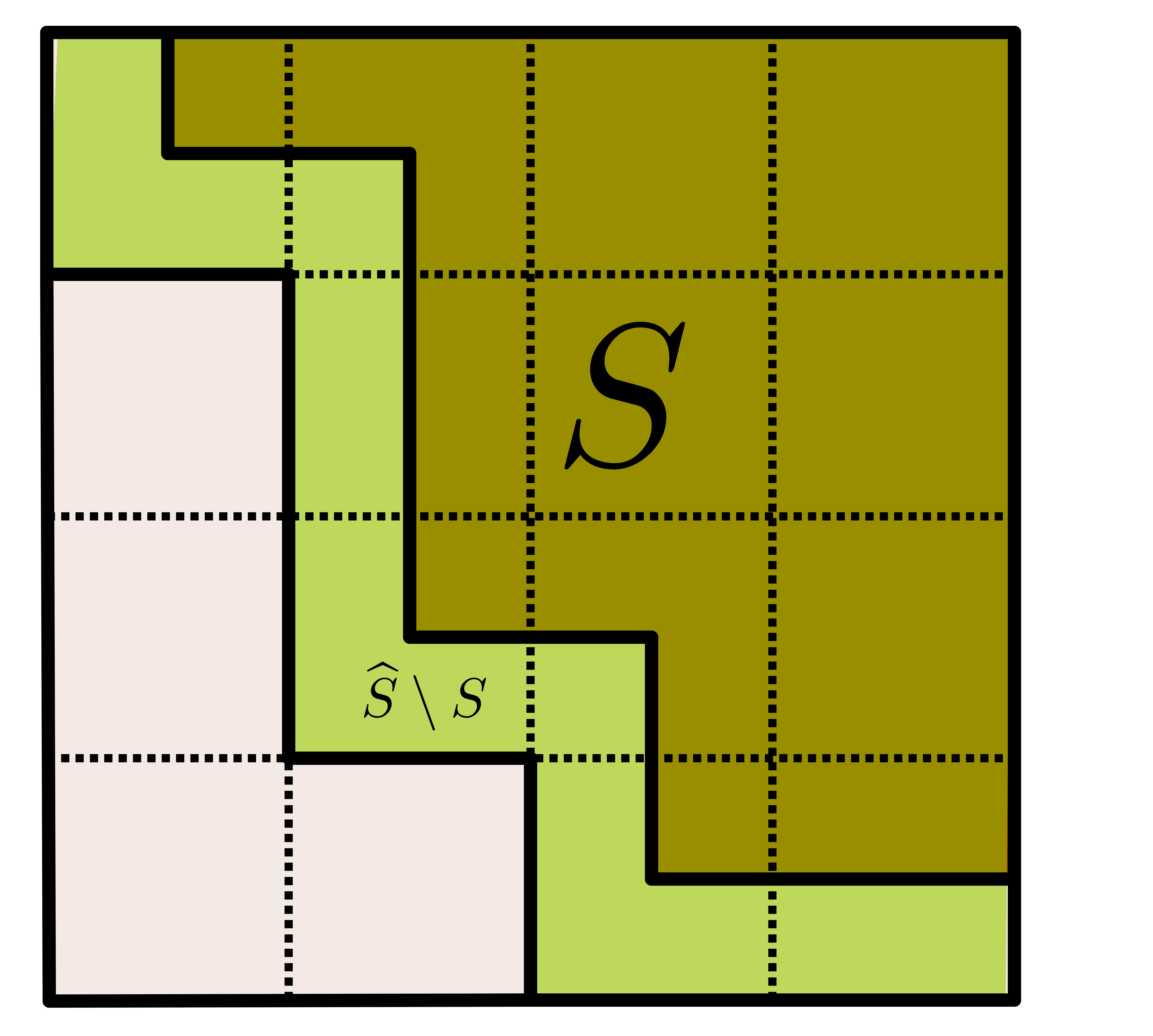
Lemma 5.2.

Fix a positive integer $Q$. Let $F=[0,N]\times[0,M]$, where $N,M$ are positive integers divisible by $Q$, and suppose that $S=F\setminus S^{\prime}$ for some tableaux region $S^{\prime}\subset F$. Let

$$\mathcal{C}_{0}=\left\{\left[\frac{Ni}{Q},\frac{N(i+1)}{Q}\right)\times\left[\frac{Mj}{Q},\frac{M(j+1)}{Q}\right)|i,j\in\{0,1\ldots,Q-1\}\right\}.$$

Let

$$\widehat{S}=\bigcup_{C\in\mathcal{C}_{0},C\cap S\neq\emptyset}C$$

be the smallest set that contains $S$ and is in the $\sigma$-algebra generated by the partition $\mathcal{C}_{0}$. Then

$$\frac{|\widehat{S}|-|S|}{NM}\leq\frac{2}{Q}.$$

Proof: There are at most $2Q$ elements of $\mathcal{C}$ that intersect both $S$ and $F\setminus S$, since these elements form a path consisting of right and down steps. In fact, there are at most $2Q-1$. See Figure 4. $\blacksquare$

Figure 4. An example, with $Q=4$ of Lemma 5.2. We can cover $\widehat{S}\setminus S$ with $7$ of the $16$ square tiles.

Definition 5.3.

($Q^{2}$-tiling and its refinement) Let $Q$ be a positive integer and suppose that

$$F=\bigcup_{m=1}^{\ell}[0,W_{m})\times[0,H_{m})$$

with

$$H_{1}>H_{2}>\ldots>H_{\ell}>0,$$

$$0<W_{1}<W_{2}<\ldots<W_{\ell}$$

and

$$W_{m}\equiv H_{m}\equiv 0\mod Q^{2}$$

for all $m\in\{1,\ldots,\ell\}$. Then we define the $Q^{2}$-tiling

$$\mathcal{C}_{0}=\mathcal{C}_{0}(F,Q)=\left\{C^{m}_{i,j}\text{ }|\text{ }i,j\in\{0,\ldots,Q-1\}\text{ and }m\in\{1,\ldots,\ell\}\right\}$$

where

$$C^{m}_{i,j}=\left[W_{m-1}+\frac{i}{Q}(W_{m}-W_{m-1}),W_{m-1}+\frac{i+1}{Q}(W_{m}-W_{m-1})\right)\times\left[\frac{j}{Q}H_{m},\frac{j+1}{Q}H_{m}\right)$$

where $W_{0}=0$. We may refine $\mathcal{C}_{0}$ as follows: Let $\mathcal{Y}=\mathcal{Y}(F,Q)$ be the set of integers which appear as a $y$ ordinate of some corner of a cell $C^{m}_{i,j}$, in other words

$$\mathcal{Y}=\left\{\frac{j}{Q}H_{m}\text{ }|\text{ }m\in\{1,\ldots,\ell\},j\in\{0,1,\ldots,Q\}\right\}.$$

Now write

$$\mathcal{Y}=\{0=y_{1}<y_{2}<\ldots<y_{|\mathcal{Y}|}\}$$

and let $\mathcal{H}=\{F\cap\left(\mathbb{R}\times[y_{r},y_{r+1})\right)\text{ }|\text{ }r\in\{0,1,\ldots,Q-1\}\}$ which is a partition of $F$. Define the refined $Q^{2}$-tiling of $F$ to be the common refinement

$$\mathcal{C}=\mathcal{C}(F,Q)=\mathcal{C}_{0}\lor\mathcal{H}$$

of the partitions $\mathcal{C}_{0}$ and $\mathcal{H}$ of $F$. More explicitly,

$$\mathcal{C}=\mathcal{C}(F,Q)=\left\{C^{m}_{i,j}\cap\mathbb{R}\times[y_{r},y_{r+1})\text{ }|\text{ }C^{m}_{i,j}\in\mathcal{C}_{0}\text{ and }r\in\{1,\ldots,|\mathcal{Y}|-1\}\right\}\setminus\{\emptyset\}.$$

Figure 5. An example, with $Q=4$, of refining $\mathcal{C}_{0}$ to $\mathcal{C}$.

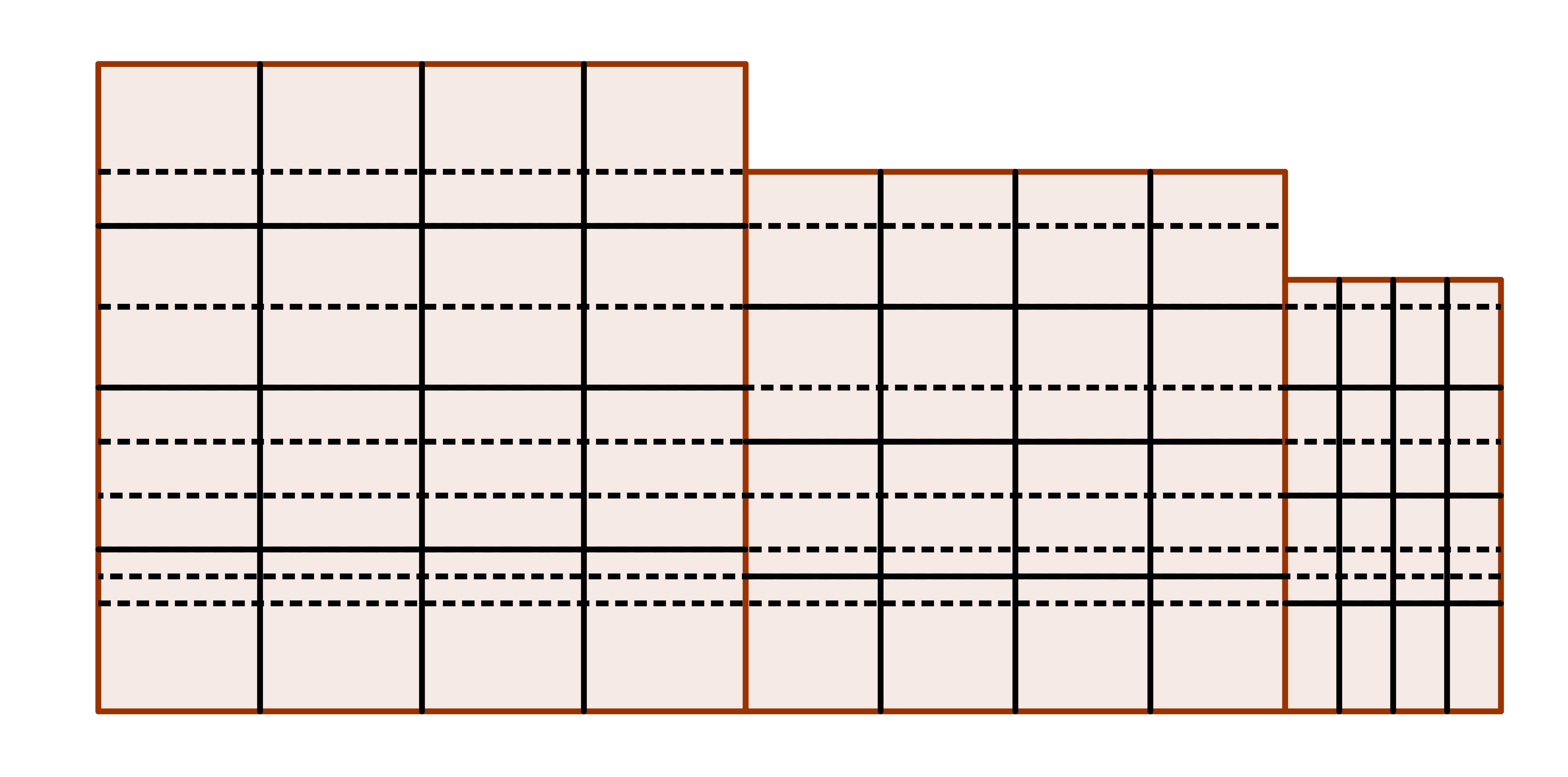
Note that the elements of $\mathcal{C}$ are rectangles with both side lengths integers divisible by $Q$, and thus contain at least $Q^{2}$ elements of $\mathbb{N}^{2}$.

Naturally, we may identify $\mathcal{C}$ with a tableau $T=T(F,Q)\subset\mathbb{N}^{2}$ by constructing a bijection $\psi:\mathcal{C}\to T$ as follows:

1. $\psi^{-1}(0,0)$ is the unique element of $\mathcal{C}$ which contains $(0,0)$.

2. $\psi^{-1}(i+1,j)$ is the element to the right of $\psi^{-1}(i,j)$ and $\psi^{-1}(i,j+1)$ is the element just above $\psi^{-1}(i,j)$. (Note: We refined $\mathcal{C}_{0}$ to $\mathcal{C}$ precisely so that the notion of right is well defined.)

A set of the form $\bigcup\psi^{-1}(T^{\prime})$ (we use the notation $\bigcup X=\bigcup_{x\in X}x$), for some tableau $T^{\prime}\subset T$, will be called a $\mathcal{C}$-measurable subtableau region. In general, a union of elements of $\mathcal{C}$ will be called a $\mathcal{C}$-measurable set.

Remark 5.4.

All $\mathcal{C}$-measurable subtableau regions contain the element of $\mathcal{C}$ that contains $(0,0)$. This element is precisely

$$[0,\frac{1}{Q}W_{1})\times[0,\frac{1}{Q}H_{\ell}).$$

Hence, each $\mathcal{C}$-measurable subtableau region is a union of rectangles of width at least $\frac{1}{Q}W_{1}$ and height $\frac{1}{Q}H_{\ell}$.

Lemma 5.5.

($\mathcal{C}$-measurable approximations) Fix a positive integer $Q$ and a $Q^{2}$-tableau region $F$. Suppose that $S\subset F$ is of the form

$$S=F\setminus F^{\prime}$$

where $F^{\prime}\subset F$ is a tableau region. Let

$$\widetilde{S}=\bigcup_{C\in\mathcal{C},C\cap S\neq\emptyset}C$$

be the smallest subset of $F$ that contains $S$ and may be written as a union of elements of $\mathcal{C}=\mathcal{C}(F,Q)$. Then

$$\frac{|\widetilde{S}\setminus S|}{|F|}\leq\frac{2}{Q}.$$

Proof: We will use the setup from Definition 5.3 above (i.e. the parameters $m$, $H_{i}$, $W_{i}$ etc.). For each $m\in\{1,\ldots,\ell\}$ define

$$U_{m}=[W_{m-1},W_{m})\times[0,H_{m})=\bigcup_{(i,j)\in\{0,1,\ldots Q-1\}^{2}}C^{m}_{i,j}.$$

Apply Lemma 5.2 to $S\cap U_{m}\subset U_{m}$ to get

$$|(\widetilde{S}\setminus S)\cap U_{m}|\leq|(\widehat{S}\setminus S)\cap U_{m}|\leq\frac{2|U_{m}|}{Q}$$

where $\widehat{S}\supset\widetilde{S}$ is the smallest subset of $F$ that contains $S$ and may be written as a union of elements of $\mathcal{C}_{0}$. Since $F=\bigsqcup_{m=1}^{\ell}U_{m}$ we are done by summing this estimate over $m\in\{1,\ldots,\ell\}$. $\blacksquare$

Lemma 5.6 (Trimming a set of points).

Fix a positive integer $Q$, a $Q^{2}$-tableaux region $F$ and $A\subset F\cap\mathbb{N}^{2}$. Let $\mathcal{C}=\mathcal{C}(F,Q)$. Define

$$\alpha=\inf\left\{\frac{|A\cap F^{\prime}|}{|F^{\prime}|}\text{ }|\text{ }F^{\prime}\subset F\text{ is a non-empty $\mathcal{C}$-measurable subtableau region}\right\}.$$

Then there exists $A^{\prime}\subset A$ such that

1. For $\mathcal{C}$-measurable subtableau regions $F^{\prime}\subsetneqq F$ we have

   $$\frac{|A^{\prime}\cap(F\setminus F^{\prime})|}{|F\setminus F^{\prime}|}\leq\alpha+\frac{1}{Q^{2}}.$$

2. $$\frac{|A^{\prime}\cap F|}{|F|}\geq\alpha.$$

Proof: $T=T(F,Q)\subset\mathbb{N}^{2}$ be the corresponding subtableau and let $\psi:\mathcal{C}\to T$ be the bijection constructed in Definition 5.3. Apply the Trimming Lemma (Lemma 4.1) to the tableaux $T$, the measure given by $\mu(\{t\})=|\psi^{-1}(t)|$ for $t\in T$ and the map $\rho:T\to[0,1]$ given by

$$\rho(t)=\frac{|A\cap\psi^{-1}(t)|}{|\psi^{-1}(t)|}$$

to obtain $\rho^{\prime}:T\to[0,1]$ such that

1. $\rho^{\prime}\leq\rho$

2. For all tableaux $T^{\prime}\subsetneqq T$, we have

   $$\frac{1}{|\bigcup\psi^{-1}(T\setminus T^{\prime})|}\sum_{t\in T\setminus T^{\prime}}|\psi^{-1}(t)|\rho^{\prime}(t)\leq\alpha.$$

3. $$\frac{1}{|F|}\sum_{t\in T}|\psi^{-1}(t)|\rho^{\prime}(t)\geq\alpha.$$

Since each element of $\mathcal{C}$ is a rectangle with both sidelengths multiples of $Q$, we may find $A^{\prime}\subset A$ such that, for all $t\in T$,

$$\rho^{\prime}(t)\leq\frac{|A^{\prime}\cap\psi^{-1}(t)|}{|\psi^{-1}(t)|}\leq\rho^{\prime}(t)+\frac{1}{Q^{2}}.$$

$\blacksquare$

We use the notation $y(a,b)=b$.

Lemma 5.7.

Fix a positive integer $Q$, a $Q^{2}$-tableaux region $F$ and $A\subset F\cap\mathbb{N}^{2}$ and let

$$S=\bigcup_{a\in A}(a+[0,\infty)^{2})\cap F.$$

Then there exists a positive integer $J$ and a sequence $a_{1},a_{2},\ldots,a_{J}\in A$ such that

$$y(a_{j})\leq y(a_{j-1})-Q$$

and

$$G:=\bigcup_{j=1}^{J}(a_{j}+[0,\infty)^{2})\cap F$$

satisfies

$$\frac{|S|-|G|}{|F|}\leq\frac{3}{Q}.$$

Proof: Note that $S=F\setminus F^{\prime}$ for some tableau region $F^{\prime}$. As in Lemma 5.5 we let

$$\widetilde{S}=\bigcup_{C\in\mathcal{C},C\cap S\neq\emptyset}C$$

be the smallest subset of $F$ that contains $S$ and may be written as a union of elements of $\mathcal{C}=\mathcal{C}(F,Q)$. So

$$\widetilde{S}=\bigsqcup_{C\in\mathcal{C}^{\prime}}C$$

for some $\mathcal{C}^{\prime}\subset\mathcal{C}$ and $\mathcal{C}^{\prime}=\psi^{-1}(T\setminus T^{\prime})$ for some tableau $T^{\prime}\subset T$, where $T=T(F,Q)$ and $\psi$ are as constructed in Definition 5.3. Now let

$$\mathcal{E}=\left\{\psi^{-1}(t_{1},t_{2})\text{ }|\text{ }(t_{1},t_{2})\in T\setminus T^{\prime}\text{ and }(t_{1}-1,t_{2})\notin T\setminus T^{\prime}\text{ and }(t_{1},t_{2}-1)\notin T\setminus T^{\prime}\right\}$$

denote the bottom-left corners of $\mathcal{C}^{\prime}$. Note that the element of $\mathcal{E}$ may be ordered vertically: we say $E$ is higher than $E^{\prime}$ if $t_{2}>t_{2}^{\prime}$ where $E=\psi^{-1}(t_{1},t_{2})$ and $E^{\prime}=\psi^{-1}(t^{\prime}_{1},t^{\prime}_{2})$. We now construct the $a_{j}$ recursively. Choose $a_{1}\in E_{1}\cap A$, where $E_{1}$ is the highest element of $\mathcal{E}$. Now suppose we have chosen $a_{1},\ldots,a_{j}$ with each $a_{j}\in A\cap E_{j}$ for some $E_{j}\in\mathcal{E}$ (by minimality of $\widetilde{S}$, $A\cap E$ is non-empty for all $E\in\mathcal{E}$). We have that $y_{r}\leq a_{j}<y_{r+1}$ for some $r=r_{j}\in\{1,\ldots,|\mathcal{Y}|-1\}$ where $\mathcal{Y}=\mathcal{Y}(F,Q)=\{y_{1}<y_{2}<\ldots<y_{|\mathcal{Y}|}\}$ is as constructed in Definition 5.3. In fact $y_{r}$ and $y_{r+1}$ are the $y$ ordinates of the corners of the element of $\mathcal{E}$ that contains $a_{j}$. Now let $E_{j+1}$ be the highest element of $\mathcal{E}$ below the horizontal line $y=y_{r-1}$ and choose $a_{j+1}\in E_{j+1}$, and if such $E_{j+1}$ does not exist then $j=J$ and we are done with our construction. Now let

$$G_{1}=(a_{1}+[0,\infty)^{2})\cap F$$

and

$$G_{j}=(a_{j}+[0,\infty)^{2})\cap F\cap\{(x,y)\in\mathbb{R}|y<y(a_{j-1})\},$$

for $1<j\leq J$ . Note that $G_{j}$ is a tableau region translated by $a_{j}$.

Figure 6. The tile $E^{\prime}_{j}$ south-east of $E_{j}$ is an element of $\mathcal{E}$, but it is not $E_{j+1}$ since it is in the row of $\mathcal{C}$ just below $E_{j}$. This ensures the desired condition that $y(a_{j+1})\leq y(a_{j})-Q$.

Now we let

$$G=\bigsqcup_{j=1}^{J}G_{j}=\bigcup_{j=1}^{J}\left(a_{j}+[0,\infty)^{2}\right)\cap F.$$

As desired, we have that (cf. Figure 6)

$$y(a_{j+1})\leq y_{r-1}\leq y_{r}-Q\leq y(a_{j})-Q.$$

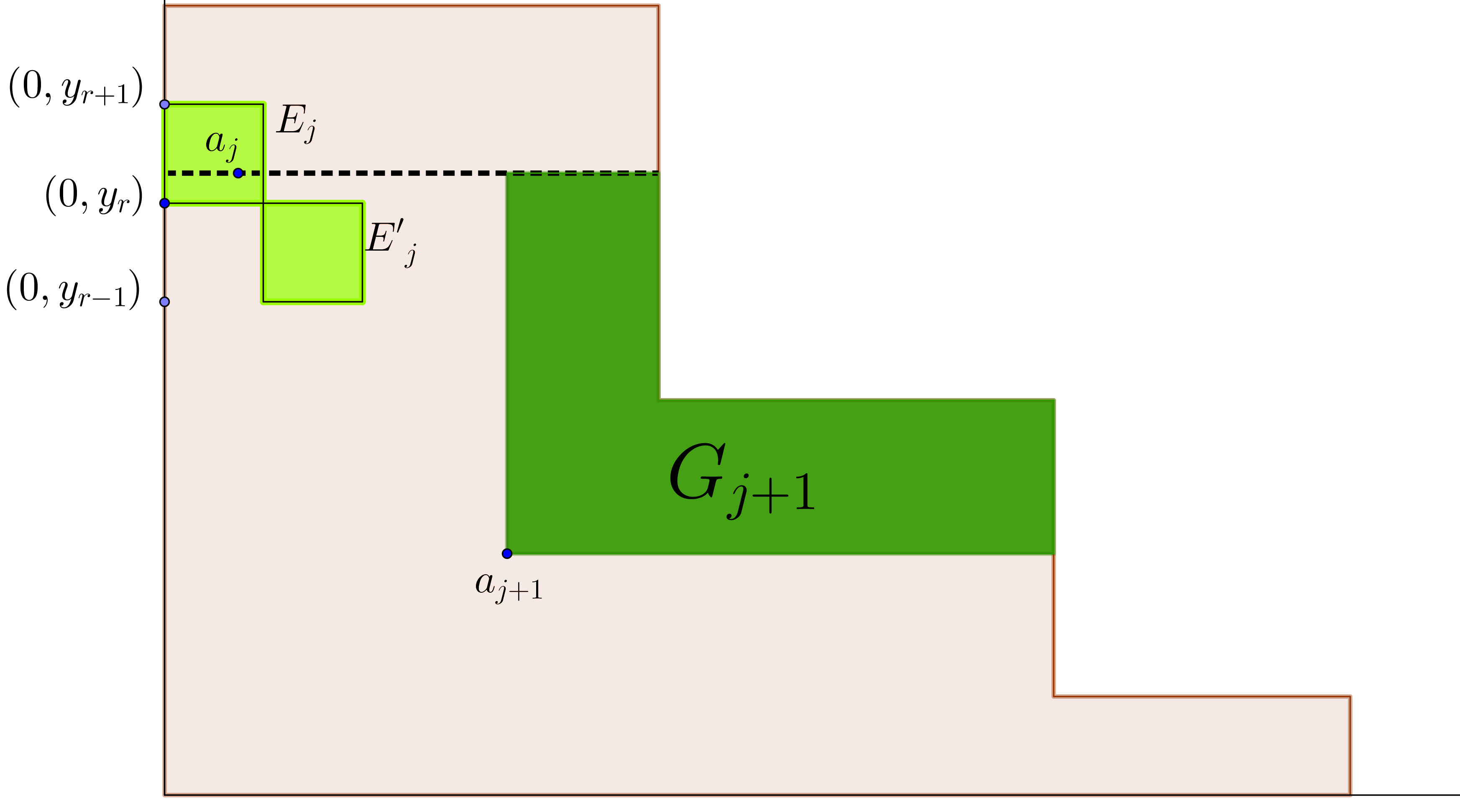
It now remains to estimate $|S\setminus G|$. To this end, let $\widetilde{G}$ denote the smallest set that contains $G$ and may be written as a union of elements of $\mathcal{C}$. We have by Lemma 5.5 that

(5.1) $$|\widetilde{G}\setminus G|\leq\frac{2|F|}{Q}$$

One may argue (see Figure 7 and its caption below) that

(5.2) $$|\widetilde{S}\setminus\widetilde{G}|\leq\frac{|F|}{Q}.$$

Combining (5.1) with (5.2) we get that

$$|S\setminus G|\leq|\widetilde{S}\setminus G|=|\widetilde{S}\setminus\widetilde{G}|+|\widetilde{G}\setminus G|\leq\frac{3|F|}{Q}$$

as desired. $\blacksquare$

Figure 7. There is at most one element of $\mathcal{E}$ below $E_{j}$ and above $E_{j+1}$, which we call (assuming it exists) $E^{\prime}_{j}$. The row of elements of $\mathcal{C}$ to the right of $E^{\prime}_{j}$ that do not intersect $G$ is a subset of $\widetilde{S}_{n}\setminus\widetilde{G}$. The union of such rows is in fact exactly $\widetilde{S}\setminus\widetilde{G}$. These rows have disjoint projections onto the $x$-axis (one can see that the projection of $E_{j+1}$ onto the $x$-axis separates the projections of the two rows shown in the figure). Thus we get that the union of all such rows has Lebesgue measure at most $\frac{1}{Q}|F|$.

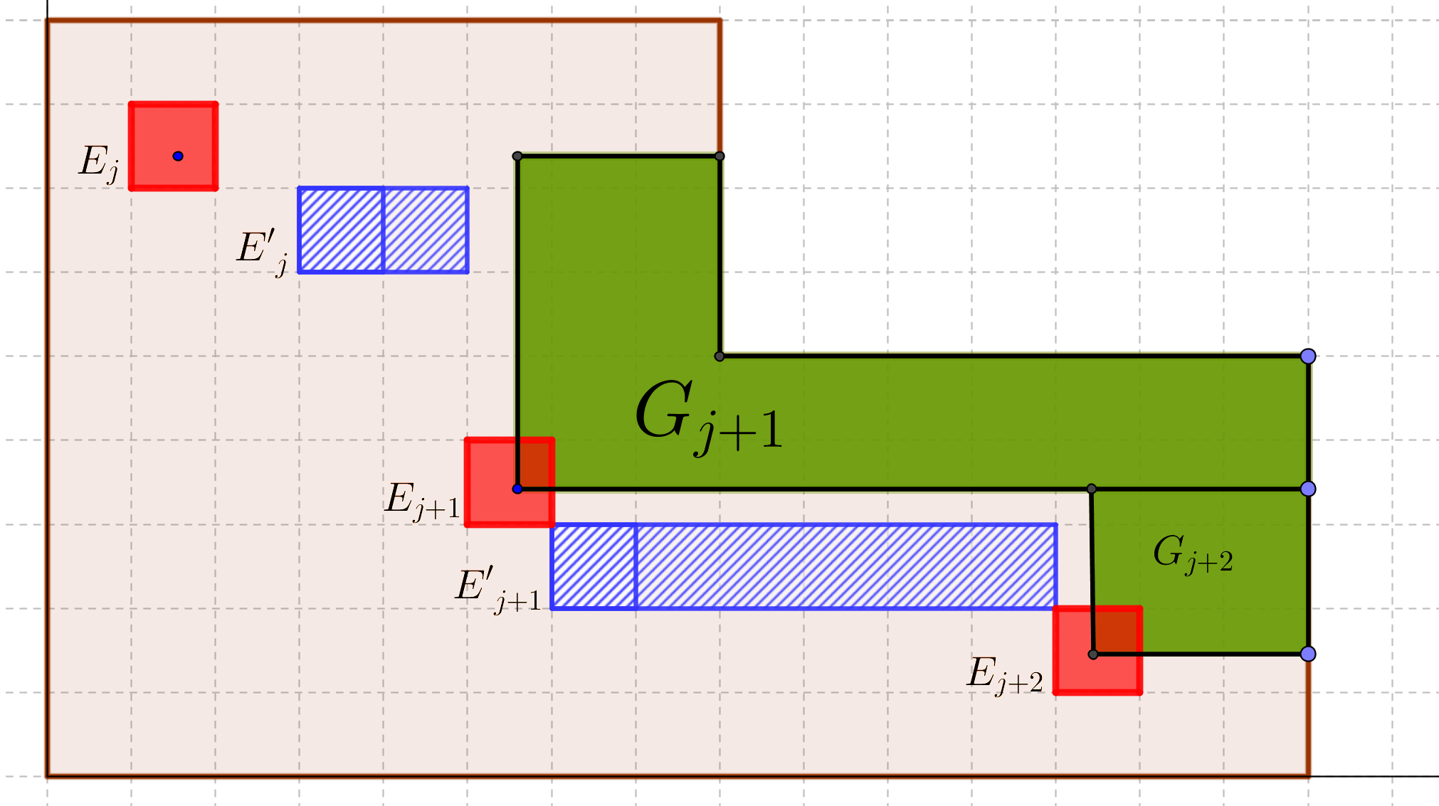
We finish this section with a simple lemma which will allow us to remove a negligible set of integral points which lie too closely to the boundary of a tableaux region.

Definition 5.8 (Bad Rows and Bad Columns).

Fix the setup in Definition 5.3 and partition

$$F=\bigsqcup_{m=1}^{\ell}U_{m}$$

where

$$U_{m}=[W_{m-1},W_{m})\times[0,H_{m})$$

for $m=1,2,\ldots,\ell$ with the convention $W_{0}=0$. Define (see Figure 8) for $m=1,\ldots,\ell$ the bad rows

$$\textbf{BadRow}_{m}=(U_{1}\cup\ldots\cup U_{m})\cap\left(\mathbb{R}\times\left[\frac{Q-1}{Q}H_{m},H_{m}\right)\right)$$

and bad columns

$$\textbf{BadCol}_{m}=\bigsqcup_{j=0}^{Q-1}C^{m}_{Q,j}=\left[W_{m-1}+\frac{Q-1}{Q}(W_{m}-W_{m-1}),W_{m}\right)\times[0,H_{m}).$$

Lemma 5.9 (Bad Rows and Columns removal).

Fix the setup in Definition 5.8 and suppose $A^{\prime}\subset F\cap\mathbb{N}^{2}$. Let

$$A_{0}=A^{\prime}\setminus\left(\bigcup_{m=1}^{\ell}\textbf{BadRow}_{m}\cup\textbf{BadCol}_{m}\right).$$

Then

$$|A_{0}|\geq|A^{\prime}|-(\ell+1)Q^{-1}|F|.$$

Proof: We have that $|\textbf{BadRow}_{m}\cap U_{j}|\leq\frac{1}{Q}|U_{j}|$ for all $m,j\in\{1,\ldots,\ell\}$ (see Figure 8) and hence $|\textbf{BadRow}_{m}|\leq\frac{1}{Q}|F|$, which means that

$$|\bigcup_{m=1}^{\ell}\textbf{BadRow}_{m}|\leq\frac{\ell}{Q}|F|.$$

On the other hand, $|\textbf{BadCol}_{m}|=\frac{1}{Q}|U_{m}|$. $\blacksquare$

Figure 8. An example of $\textbf{BadRow}_{2}$ and $\textbf{BadCol}_{3}$ with $Q=4$ and $\ell=3$. Note that $\textbf{BadRow}_{2}$ intersects exactly $\frac{1}{4}$ of $U_{2}$, strictly less than $\frac{1}{4}$ of $U_{1}$ and none of $U_{3}$.

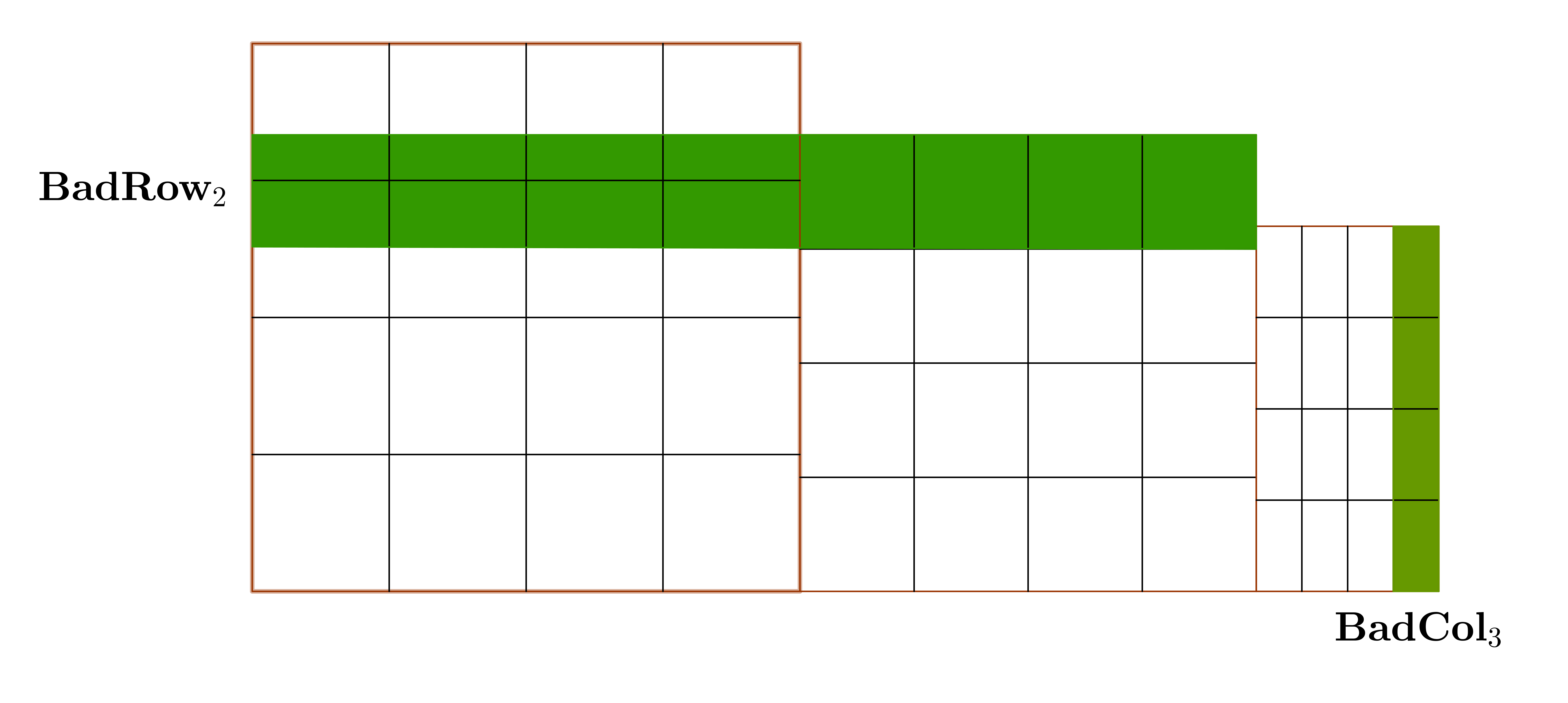
6. Proof of Theorem 1.12

As in the hypothesis of Theorem 1.12, fix $A,B\subset\mathbb{N}^{2}$ with $\alpha:=\underline{d}_{\textbf{Tab}}(A)>0$ and $(0,0)\in B$ together with integers $0<k^{\prime}<k$ and $L>0$. Now fix an integer

(6.1) $$Q\geq 4(L+1)\alpha^{-1}$$

and choose (by Lemma 3.3) a sequence

$$F_{n}=\bigcup_{m=1}^{\ell(n)}[0,W_{n,m})\times[0,H_{n,m})$$

with $\ell(n)\leq L$ such that

1. $$\lim_{n\to\infty}\frac{|(A+kB)\cap F_{n}|}{|F_{n}|}=\underline{d}_{\textbf{Tab}(L)}(A+kB)$$

2. For all $n>1$ and $1\leq m\leq\ell(n)$ we have

   $$H_{n,m}\equiv W_{n,m}\equiv 0\mod Q^{2}$$

3. $$\lim_{n\to\infty}\inf_{m\in\{1,\ldots,\ell(n)\}}W_{n,m}=\lim_{n\to\infty}\inf_{m\in\{1,\ldots,\ell(m)\}}H_{n,m}=\infty.$$

We also assume, by reordering rectangles and deleting redundant rectangles if necessary, that

$$H_{n,1}>H_{n,2}>\ldots>H_{n,\ell(n)}$$

$$W_{n,1}<W_{n,2}<\ldots<W_{n,\ell(n)}.$$

We now apply the techniques developed in Section 5 to the tableau regions $F_{n}$. Note that the $\mathcal{C}(F_{n},Q)$-measurable subtableau regions of $F_{n}$ are a union of at most $Q^{2}L^{2}$ (and thus a bounded function of $n$) rectangles with sidelengths tending to $\infty$ as $n\to\infty$ (see Remark 5.4), we thus have that

(6.2) $$\liminf_{n\to\infty}\alpha_{n}\geq\alpha$$

where

$$\alpha_{n}:=\inf\left\{\frac{|A\cap F^{\prime}|}{|F^{\prime}|}|F^{\prime}\text{ is a }\mathcal{C}(F_{n},Q)\text{-measurable subtableau region}\right\}.$$

Thus there exists $\tilde{N}$ (which depends on $Q$ and the sequence $F_{n}$, which we have fixed) such that

$$\alpha_{n}>\frac{3}{4}\alpha\text{ for all }n>\tilde{N}.$$

From here on, we fix $n>\tilde{N}$ and let $\ell=\ell(n)$, $W_{m}=W_{n,m}$, $H_{m}=H_{n,m}$ for $m\in\{1,\ldots,\ell\}$. Applying Lemma 5.6 to $F_{n}$ we obtain a subset $A^{\prime}\subset A\cap F_{n}$ such that

(6.3) $$\frac{|A^{\prime}\cap(F_{n}\setminus F^{\prime})|}{|F_{n}\setminus F^{\prime}|}\leq\alpha_{n}+\frac{1}{Q^{2}}\text{ for all }\mathcal{C}(F_{n},Q)\text{-measurable tableau }F^{\prime}\subsetneqq F_{n}.$$

and

$$\frac{|A^{\prime}|}{|F_{n}|}\geq\alpha_{n}.$$

Now let

$$A_{0}=A^{\prime}\setminus\left(\bigcup_{m=1}^{\ell}\textbf{BadRow}_{m}\cup\textbf{BadCol}_{m}\right)$$

where we have used the language of Definition 5.8. We have by Lemma 5.9 that

(6.4) $$|A_{0}|\geq|A^{\prime}|-(L+1)Q^{-1}|F_{n}|\geq(\alpha_{n}-(L+1)Q^{-1})|F_{n}|.$$

So from $\alpha_{n}>\frac{3}{4}\alpha$ and (6.1) we get that

(6.5) $$\frac{|A_{0}|}{|F_{n}|}>\frac{1}{2}\alpha$$

is bounded away from zero.

Applying the $\delta$-heavy truncated Plünnecke’s inequality (Proposition 3.2) with $\delta=Q^{-1/2}$ to the finite set $A_{0}\subset F_{n}$, we get

(6.6) $$\frac{|(A+k^{\prime}B)\cap F_{n}|}{|A_{0}|}\geq\frac{|(A_{0}+k^{\prime}B)\cap F_{n}|}{|A_{0}|}\geq(1-Q^{-1/2})\left(\frac{|(A^{\prime}_{0}+kB)\cap F_{n}|}{|A^{\prime}_{0}|}\right)^{k^{\prime}/k}$$

for some nonempty $A^{\prime}_{0}\subset A_{0}$ with

$$|A^{\prime}_{0}|\geq Q^{-1/2}|A_{0}|.$$

Now let

$$S_{n}=\bigcup_{v\in A^{\prime}_{0}}(v+[0,\infty)^{2})\cap F_{n}$$

be the smallest set that contains $A^{\prime}_{0}$ and is the complement (in $F_{n}$) of a tableau region contained in $F_{n}$. We have by Lemma 5.5 that

(6.7) $$\frac{|\widetilde{S_{n}}\setminus S_{n}|}{|F|}\leq\frac{2}{Q}$$

where $\widetilde{S_{n}}$ is the smallest $\mathcal{C}$-measurable set that contains $S_{n}$. Now note that

(6.8) $$\frac{|S_{n}|}{|F_{n}|}\geq\frac{|A^{\prime}_{0}|}{|F_{n}|}\geq\frac{Q^{-1/2}|A_{0}|}{|F_{n}|}\geq\frac{1}{2}\alpha Q^{-1/2}$$

by (6.5). Combining these two estimates gives

(6.9) $$\frac{|\widetilde{S}_{n}|}{|S_{n}|}\leq 1+4\alpha^{-1}Q^{-1/2}.$$

Also notice that $\widetilde{S}_{n}$ is the complement of a $\mathcal{C}(F_{n},Q)$-measurable tableau, and thus we may apply (6.3) to obtain

(6.10) $$\frac{|A^{\prime}_{0}|}{|\widetilde{S}_{n}|}\leq\frac{|A^{\prime}\cap\widetilde{S}_{n}|}{|\widetilde{S}_{n}|}\leq\alpha_{n}+\frac{1}{Q^{2}}.$$

Now applying the inequalities (6.6), followed by (6.4), followed by (6.10) and then finally (6.9) we obtain

$$\left(\frac{|(A+k^{\prime}B)\cap F_{n}|}{|F_{n}|}\right)^{k/k^{\prime}}$$

$$\geq\left(\frac{|A_{0}|}{|F_{n}|}(1-Q^{-1/2})\right)^{k/k^{\prime}}\frac{|(A^{\prime}_{0}+kB)\cap F_{n}|}{|A^{\prime}_{0}|}$$

$$\geq\left((\alpha_{n}-(L+1)Q^{-1})(1-Q^{-1/2})\right)^{k/k^{\prime}}\frac{|(A^{\prime}_{0}+kB)\cap F_{n}|}{|A^{\prime}_{0}|}$$

$$=\left((\alpha_{n}-(L+1)Q^{-1})(1-Q^{-1/2})\right)^{k/k^{\prime}}\frac{|\widetilde{S}_{n}|}{|A^{\prime}_{0}|}\frac{|(A^{\prime}_{0}+kB)\cap F_{n}|}{|\widetilde{S}_{n}|}$$

$$\geq\left((\alpha_{n}-(L+1)Q^{-1})(1-Q^{-1/2})\right)^{k/k^{\prime}}(\alpha_{n}+Q^{-2})^{-1}\frac{|(A^{\prime}_{0}+kB)\cap F_{n}|}{|\widetilde{S}_{n}|}$$

$$\geq\left((\alpha_{n}-(L+1)Q^{-1})(1-Q^{-1/2})\right)^{k/k^{\prime}}(\alpha_{n}+Q^{-2})^{-1}(1+4\alpha^{-1}Q^{-1/2})^{-1}\frac{|(A^{\prime}_{0}+kB)\cap F_{n}|}{|S_{n}|}$$

which, by letting $\lambda(n,Q)$ denote the factor before $\frac{|(A^{\prime}_{0}+kB)\cap F_{n}|}{|S_{n}|}$, we rewrite as

(6.11) $$\left(\frac{|(A+k^{\prime}B)\cap F_{n}|}{|F_{n}|}\right)^{k/k^{\prime}}\geq\lambda(n,Q)\frac{|(A^{\prime}_{0}+kB)\cap F_{n}|}{|S_{n}|}.$$

Using $\liminf_{n\to\infty}\alpha_{n}\geq\alpha$ (justified in (6.2)) it is an easy calculation to show that

(6.12) $$\liminf_{Q\to\infty}\liminf_{n\to\infty}\lambda(n,Q)\geq\alpha^{\frac{k}{k^{\prime}}-1}.$$

We now wish to show that

$$\liminf_{Q\to\infty}\liminf_{n\to\infty}\frac{|(A^{\prime}_{0}+kB)\cap F_{n}|}{|S_{n}|}\geq\underline{d}_{\textbf{Tab}(L)}(kB).$$

Note that this holds trivially in the case that $kB=\mathbb{N}^{2}$, as in this case we have that $|(A^{\prime}_{0}+kB)\cap F_{n}|=|S_{n}\cap\mathbb{Z}^{2}|$ and thus

(6.13) $$\frac{|(A^{\prime}_{0}+kB)\cap F_{n}|}{|S_{n}|}=1.$$

We now return to the general case. Apply Lemma 5.7 to $A^{\prime}_{0}$ and $S_{n}$ to obtain $a_{1},a_{2},\ldots,a_{J}\in A$ with

$$y(a_{j})\leq y(a_{j-1})-Q$$

such that the set

$$G:=\bigcup_{j=1}^{J}\left(a_{j}+[0,\infty)^{2}\right)\cap F_{n}$$

satisfies

(6.14) $$\frac{|S\setminus G|}{|F_{n}|}\leq\frac{3}{Q}.$$

Now decompose

$$G=\bigsqcup_{j=1}^{J}G_{j}$$

where

$$G_{1}=(a_{1}+[0,\infty)^{2})\cap F_{n}$$

and

$$G_{j}=(a_{j}+[0,\infty)^{2})\cap F_{n}\cap\{(x,y)\in\mathbb{R}|y<y(a_{j-1})\},$$

for $1<j\leq J$. Note that $G_{j}$ is a tableau region translated by $a_{j}$ (cf. Figure 6 in the proof of Lemma 5.7).

Claim: Each $G_{j}$ is a union of at most $L$ rectangles with bottom corner $a_{j}$, each with sidelengths at least $Q$.

Proof of Claim: Writing $a_{j}=(x,y)$, we can write (see Figure 6)

$$G_{j}=\bigcup_{m}[x,W_{m})\times[y,\min\{y(a_{j-1}),H_{m}\})$$

where the union is over $m\in\{1,\ldots,\ell\}$ such that $x<W_{m}$ and $y<H_{m}$ (for $j=1$, we omit the $y(a_{j-1})$). For such $m$, we have that $W_{m}-x\geq Q$ and $H_{m}-y\geq Q$ since $a_{j}$ avoids $\textbf{BadRow}_{m}$ and $\textbf{BadCol}_{m}$, respectively. We also have $y(a_{j-1})-y\geq Q$ by construction of the $a_{j}$. This completes the proof of the Claim. $\square$

This claim implies that

$$\frac{|(A^{\prime}_{0}+kB)\cap G_{j}|}{|G_{j}|}\geq\frac{|(a_{j}+kB)\cap G_{j}|}{|G_{j}|}\geq\underline{d}_{\textbf{Tab}(L)}(kB)-\delta(Q)$$

where

$$\delta:\mathbb{N}\to[0,\infty)$$

is a map (it depends on $kB$, but not $n$) such that $\lim_{Q\to\infty}\delta(Q)=0$. We thus have that

$$\frac{|(A^{\prime}_{0}+kB)\cap G|}{|G|}\geq\underline{d}_{\textbf{Tab}(L)}(kB)-\delta(Q).$$

Now combining (6.14) with (6.8) gives

$$\frac{|G|}{|S_{n}|}\geq 1-6\alpha^{-1}Q^{-1/2}$$

and so we have that

$$\frac{|(A^{\prime}_{0}+kB)\cap S_{n}|}{|S_{n}|}\geq \frac{|(A^{\prime}_{0}+kB)\cap G|}{|S_{n}|}$$

$$\geq \frac{|G|}{|S_{n}|}(\underline{d}_{\textbf{Tab}(L)}(kB)-\delta(Q))$$

$$\geq \left(1-6\alpha^{-1}Q^{-1/2}\right)(\underline{d}_{\textbf{Tab}(L)}(kB)-\delta(Q)).$$

So in summary, we have (see (6.11)) that

$$\left(\frac{|(A+k^{\prime}B)\cap F_{n}|}{|F_{n}|}\right)^{k/k^{\prime}}\geq\lambda(n,Q)\left(1-6\alpha^{-1}Q^{-1/2}\right)(\underline{d}_{\textbf{Tab}(L)}(kB)-\delta(Q)).$$

Finally, this completes the proof as

$$\underline{d}_{\textbf{Tab}(L)}(A+k^{\prime}B) =\liminf_{n\to\infty}\frac{|(A+k^{\prime}B)\cap F_{n}|}{|F_{n}|}$$

$$\geq\liminf_{n\to\infty}\lambda(n,Q)^{k^{\prime}/k}\left(1-6\alpha^{-1}Q^{-1/2}\right)^{k^{\prime}/k}(\underline{d}_{\textbf{Tab}(L)}(kB)-\delta(Q))^{k^{\prime}/k}$$

from which we deduce Theorem 1.12 by letting $Q\to\infty$ and using (6.12). $\blacksquare$

7. Further questions

We now list some related open problems. We start by recalling the main motivating question of this paper.

Question 7.1.

For $A,B\subset\mathbb{N}^{2}$ and positive integers $k^{\prime}<k$, is it true that

$$\underline{d}_{\textbf{Rect}}(A+k^{\prime}B)\geq\underline{d}_{\textbf{Rect}}(A)^{1-\frac{k^{\prime}}{k}}\underline{d}_{\textbf{Rect}}(kB)^{\frac{k^{\prime}}{k}}?$$

One may state a finitistic version of this problem by considering the finitistic and multidimensional analogue of the classical Schnirelmann density given by

$$\sigma_{N,M}(A)=\min_{0\leq n\leq N,0\leq m\leq M}\frac{A\cap([0,n]\times[0,m])}{(n+1)(m+1)}$$

for $A\subset\mathbb{N}^{2}\cap([0,N]\times[0,M])$.

Question 7.2 (Multidimensional Schnirelmann density Plünnecke inequality).

Fix positive integers $N$ and $M$. If $A,B\subset\mathbb{N}^{2}\cap([0,N]\times[0,M])$, with $(0,0)\in B$, then is it true that

$$\sigma_{N,M}(A+k^{\prime}B)\geq\sigma_{N,M}(A)^{1-\frac{k^{\prime}}{k}}\sigma_{N,M}(kB)^{\frac{k^{\prime}}{k}}$$

for positive integers $k^{\prime}<k$ ?

We note that the $M=0$ case is precisely Plünnecke’s classical inequality for Schnirelmann density in $\mathbb{N}$ (Theorem 1.2). Even the following special case is not clear.

Question 7.3.

What is the answer to Question 7.2 in the case $M=1$?

Appendix A Densities of fractal sets

We will now prove our formulae for $\underline{d}_{\textbf{Tab}}(A)$ and $\underline{d}_{\textbf{Rect}}(A)$ (Proposition 1.15) for fractal sets $A$. We will use the notation $[a,b)=\{x\in\mathbb{Z}|a\leq x<b\}$. So let us fix in this section $A=A(P,N)$ a fractal set, where $N\in\mathbb{N}$ and $P\subset\{0,1,\ldots,N\}^{2}$ is a pattern. We also fix the data $A_{k}\subset\mathcal{P}_{k}$ and $u_{k}\in\mathbb{N}$ given in Definition 1.14.

A.1. Rectangular density

We first deal with the rectangular case; so in this subsection we fix a Følner sequence of the form $F_{n}=[0,W_{n})\times[0,H_{n})\cap\mathbb{N}^{2}$, $n=1,2,3\ldots$ where $W_{n},H_{n}\to\infty$. It is enough to show that

(A.1) $$\liminf_{n\to\infty}\frac{|A\cap F_{n}|}{|F_{n}|}\geq\alpha:=\min\left\{\frac{|P\cap I|}{|I|}\text{ }|\text{ }I=[0,x]\times[0,y]\cap\mathbb{N}^{2}\text{ for some }x,y\in\{0,1,\ldots,N\}\right\}$$

as it is easy to see that

$$\alpha\geq\underline{d}_{\textbf{Tab}}(A)$$

by considering the Følner sequence

$$F_{k}=[0,(x+1)u_{k})\times[0,(y+1)u_{k})$$

where $(x,y)\in\{0,1\ldots,N\}^{2}$ attain the minimum in (A.1).

Define the core of $F_{n}$ to be the set

$$F^{o}_{n}=F_{n}\cap[0,(N+1)u_{k_{n}})^{2}$$

where $k_{n}$ is the largest positive integer such that $[0,u_{k_{n}})^{2}\subset F_{n}$. Our goal is to show the following two inequalities

(A.2) $$\liminf_{n\to\infty}\frac{|F^{o}_{n}\cap A|}{|F^{o}_{n}|}\geq\alpha$$

(A.3) $$\liminf_{n\to\infty}\frac{|(F_{n}\setminus F^{o}_{n})\cap A|}{|F_{n}\setminus F^{o}_{n}|}\geq\alpha$$

which will imply the formula for rectangular density. The key ingredient is the following Perturbation Lemma.

Lemma A.1 (Perturbation Lemma).

Suppose $F=[0,W)\times[0,H)\cap\mathbb{N}^{2}$ where $(W,H)\in\mathbb{N}^{2}$. Suppose that for some $k\in\mathbb{N}$ we have that $u_{k}\leq H\leq u_{k+1}$ and $W\leq u_{k+1}$. Then there exists $\tilde{H}\in\{iu_{k}|i\in\{1,2,\ldots N+1\}\}$ such that

$$\frac{|\tilde{F}\cap A|}{|\tilde{F}|}\leq\frac{|F\cap A|}{|F|}$$

where

$$\tilde{F}=[0,W)\times[0,\tilde{H})\cap\mathbb{N}^{2}.$$

Proof: Since $F\setminus[0,(N+1)u_{k})^{2}\subset A$, it suffices to consider the case where $W,H\leq(N+1)u_{k}$. Write $H=qu_{k}+r$ where $r\in\{0,1,\ldots u_{k}-1\}$ and $q\in\{1,\ldots,(N+1)\}$. If $q=N+1$ then we must have $r=0$, which means that we can set $\tilde{H}:=H=(N+1)u_{k}$ and we are done with the proof, so let us now assume $q<N+1$. The quantity

$$\frac{|A\cap([0,W)\times\{t\})|}{|W|}$$

is constant for $t\in\{0,1,\ldots u_{k}-1\}$ since the sets $A\cap\left([0,W)\times\{t\}\right)$ all have the same projection onto the $x$-axis (see Figure 9). We denote this constant by $C$.

Figure 9. The cross sections $A\cap([0,W)\times\{t\})$ and $A\cap([0,W)\times\{t^{\prime}\})$ are the same upto a vertical translation.

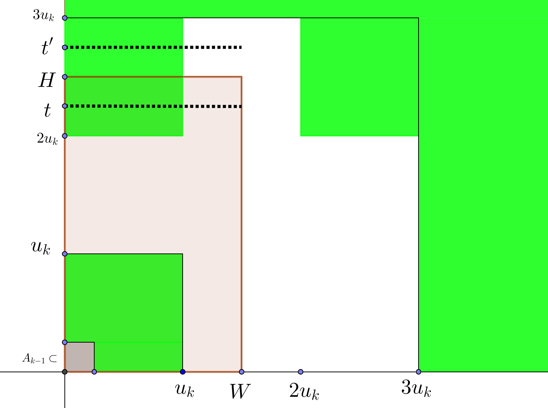
It will be convenient to use the notation

$$d(X|Y)=\frac{|X\cap Y|}{|Y|}$$

where $X,Y$ are finite sets. Hence if we define, for $t=0,1,\ldots u_{k}$, the expression

$$g(t):=d\left(A|[0,W)\times[0,qu_{k}+t)\right)=\frac{|A\cap[0,W)\times[0,qu_{k}+t)|}{W(qu_{k}+t)}$$

then we can rewrite it as a convex combination

(A.4) $$g(t)=\lambda\cdot d\left(A|[0,W)\times[0,qu_{k})\right)+(1-\lambda)C$$

where

$$\lambda=\frac{Wqu_{k}}{W(qu_{k}+t)}.$$

Now notice that $g(t)$ is a monotonic function of $\lambda$, and thus a monotonic function of $t$. Hence the minimum of $g(t)$ occurs at either $t=0$ or $t=u_{k}$. If it occurs at $t=0$, we set $\tilde{H}=qu_{k}$ while if it occurs at $t=u_{k}$, we set $\tilde{H}=(q+1)u_{k}$. We thus get that

$$\frac{|A\cap\tilde{F}|}{|\tilde{F}|}\leq\frac{|F\cap A|}{|F|}$$

where $\tilde{F}=[0,W)\times[0,\tilde{H}).$ $\blacksquare$

Remark A.2.

In Lemma A.1 one may drop the hypothesis that $u_{k+1}\geq H$ if one replaces $A$ with $\mathcal{P}_{k}$. The reason is that this hypothesis was only used to show that the cross section density $C$ was constant with respect to $t$, which is not an issue if one replaces $A$ with $\mathcal{P}_{k}$. This variation of the lemma will also be useful.

Lemma A.3 (Perturbing both sides).

In the situation of Lemma A.1 if it is also the case that $W\geq u_{k}$, then there exists $\tilde{H},\tilde{W}\in\{iu_{k}\text{ }|\text{ }i\in\{1,2,\ldots N+1\}\}$ such that

$$\frac{|\tilde{F}\cap A|}{|\tilde{F}|}\leq\frac{|F\cap A|}{|F|}$$

where

$$\tilde{F}=[0,\tilde{W)}\times[0,\tilde{H})\cap\mathbb{N}^{2}.$$

Proof: After applying Lemma A.1, apply it again with dimensions reversed. $\blacksquare$

We may apply Lemma A.3 with $F=F^{o}_{n}$ (and $k=k_{n}$) to obtain the corresponding rectangle $\tilde{F}^{o}_{n}$ which satisfies

$$\frac{|\tilde{F}^{o}_{n}\cap A|}{|\tilde{F}^{o}_{n}|}\leq\frac{|F^{o}_{n}\cap A|}{|F^{o}_{n}|}.$$

However, by definition of $\alpha$, it is clear that

$$\frac{|\tilde{F}^{o}_{n}\cap\mathcal{P}_{k_{n}}|}{|\tilde{F}^{o}_{n}|}\geq\alpha.$$

But since $\frac{u_{k}}{u_{k-1}}\to\infty$, we have that

$$|\frac{|\tilde{F}^{o}_{n}\cap\mathcal{P}_{k_{n}}|}{|\tilde{F}^{o}_{n}|}-\frac{|\tilde{F}^{o}_{n}\cap A|}{|\tilde{F}^{o}_{n}|}|\to 0\text{ as }n\rightarrow\infty,$$

which shows (A.2). Now we turn to showing (A.3). Suppose, WLOG, that $H_{n}\geq W_{n}$, thus

$$F_{n}\setminus F^{o}_{n}=[0,W_{n})\times[(n+1)u_{k_{n}},H_{n}).$$

Now if we are in the degenerate case where $H_{n}\leq u_{k_{n}+1}$ then in fact $F_{n}\setminus F^{o}_{n}=\emptyset$ and so we are done. If however $H_{n}>u_{k_{n}+1}$ then $\frac{|F_{n}\setminus F^{o}_{n}|}{|F_{n}|}\geq 1-\epsilon_{n}$, for some $\epsilon_{n}\to 0$, which means that we may replace $F_{n}\setminus F^{o}_{n}$ with $F_{n}$ in (A.3) to get a logically equivalent statement. So we apply Lemma A.1 (with $k$ being the largest integer such that $H_{n}\geq u_{k}$ and $F=F_{n}$) and argue as before.

Remark A.4.

We did not really need to consider the definition of a core, but this notion will be useful in establishing the formula for Tableaux density in the next subsection.

A.2. Tableaux density

We will now prove the formula for $\underline{d}_{\textbf{Tab}}(A)$ for the fractal set $A=A(N,P)$. In this subsection we fix an integer $L\geq 1$ and a Følner sequence

$$F_{n}=\bigcup_{j=1}^{L}\left[0,W_{n,j}\right)\times\left[0,H_{n,j}\right).$$

Now let

$$\beta=\min\left\{\frac{|P\cap T|}{|T|}\text{ }|\text{ }T\subset\{0,1,\ldots,N\}^{2}\text{ is a tableaux }\right\}.$$

We wish to show that

$$\beta\leq\liminf_{n\to\infty}\frac{|A\cap F_{n}|}{|F_{n}|},$$

where $H_{n,j}$ is decreasing and $W_{n,j}$ is increasing in $j$, for each fixed $n$.

Exactly as in Section A.1, we define the core of $F_{n}$ to be the set

$$F^{o}_{n}=F_{n}\cap[0,u_{1+k_{n}})^{2}$$

where $k_{n}$ is the largest positive integer such that $[0,u_{k_{n}})^{2}\subset F_{n}$. As before, we start with a perturbation lemma. We note again that (since $\frac{u_{k}}{u_{k-1}}\to\infty$)

(A.5) $$\lim_{n\to\infty}\left|\frac{|A\cap F_{n}|}{|F_{n}|}-\frac{|\mathcal{P}_{k_{n}}\cap F_{n}|}{|F_{n}|}\right|=0.$$

Lemma A.5 (Order $L$ perturbation lemma).

Let

$$F=\bigcup_{j=1}^{L}[0,W_{j})\times[0,H_{j})$$

for some positive integers $H_{1}\geq\cdots\geq H_{L}$ and $W_{1}\leq\cdots W_{L}$. Now suppose that there exists a positive integer such that $k$ be the largest positive integer such that $[0,u_{k})^{2}\subset F\subset[0,u_{k+1})^{2}$. Then, for each $j=1,\ldots,L$, there exists $\tilde{W}_{j},\tilde{H}_{j}\in\{iu_{k}\text{ }|\text{ }i\in\{1,\ldots,N+1\}\}$ such that

$$\frac{|\mathcal{P}_{k}\cap\tilde{F}|}{|\tilde{F}|}\leq\frac{|\mathcal{P}_{k}\cap F|}{|F|}$$

where

$$\tilde{F}=\bigcup_{j=1}^{L}[0,\tilde{W}_{j})\times[0,\tilde{H}_{j})$$

and $\tilde{H}_{1}\geq\cdots\geq\tilde{H}_{L}$ and $\tilde{W}_{1}\leq\cdots\leq\tilde{W}_{L}$

Proof (Sketch): The $L=1$ case is essentially Lemma A.3 (see Remark A.2. In fact, in this proof we always use the formulation given in that remark). For $L>1$ we proceed by induction as follows. Let $H=H_{1},W=W_{1}$ and apply Lemma A.1 to $[0,H)\times[0,W)$ to produce $\tilde{H}$. Now if $\tilde{H}\geq H_{2}$ then set $\tilde{H}_{1}=\tilde{H}$. However if $\tilde{H}_{1}<H_{2}$ then we see, by the same convexity argument as in Lemma A.1, that

$$\frac{|\mathcal{P}_{k}\cap F^{\prime}|}{|F^{\prime}|}\leq\frac{|\mathcal{P}_{k}\cap F|}{|F|}$$

where

$$F^{\prime}=\bigcup_{i=1}^{L-1}[0,W_{i+1})\times[0,H_{i+1})$$

and so we are done (in this case) by applying the induction hypothesis to $F^{\prime}$. We construct $\tilde{H}_{2},\ldots\tilde{H}_{L}$ by continuing in this way (for example, to get $\tilde{H}_{2}$ one applies the same technique to $[W_{1},W_{2})\times[0,H_{2})$). $\blacksquare$

The formula for the tableaux density of $A$ now follows by applying Lemma A.5 to the core of $F_{n}$ (with $k=k_{n}$) and arguing as we did in the case of rectangular density.

Appendix B Density of cartesian products

We now prove the property

(B.1) $$\underline{d}_{\textbf{Tab}(L)}(A\times B)=\underline{d}(A)\underline{d}(B)$$

for $A,B\subset\mathbb{N}$ and $L\in\mathbb{Z}_{>0}$. It is clear that

$$\underline{d}_{\textbf{Tab}(L)}(A\times B)\leq\underline{d}(A)\underline{d}(B)$$

and so we focus on proving the reverse inequality. We do this by induction on $L$. The $L=1$ case is clear, so let us suppose that $L>0$ and that the property holds for $\textbf{Tab}(L-1)$. Let $A,B\subset\mathbb{N}$ and let

$$F_{n}=\mathbb{N}^{2}\cap\bigcup_{i=1}^{L}[0,W_{n,i})\times[0,H_{n,i})$$

be a sequence (where $W_{n,1}<\cdots<W_{n,L}$ and $H_{n,1}>\cdots>H_{n,L}$ are positive integers with $W_{n,i},H_{n,i}\to\infty$ as $n\to\infty$ for each $i$) such that

$$\underline{d}_{\textbf{Tab}(L)}(A\times B)=\lim_{n\to\infty}\frac{|(A\times B)\cap F_{n}|}{|F_{n}|}.$$

Now we assume, by passing to a subsequence if necessary, that the limit

$$\alpha_{i}:=\lim_{n\to\infty}\frac{|A\cap[W_{n,i},W_{n,i+1})|}{W_{n,i+1}-W_{n,i}}$$

exists for $i=0,\ldots,L-1$ (where $W_{n,0}=0$). Likewise, we assume that

$$\beta_{j}:=\lim_{n\to\infty}\frac{|B\cap[H_{n,j+1},H_{n,j+2})|}{H_{n,j+2}-H_{n,j+1}}$$

exists for $j=0,\ldots,L-1$ (where $H_{n,L+1}=0$). Using the fact that $\alpha_{0}\geq\underline{d}(A)$ and $\beta_{L-1}\geq\underline{d}(B)$ we can easily deduce that one of the following must occur:

1. There exists $r\in\{0,\ldots,L-1\}$ such that $\alpha_{r}\geq\underline{d}(A)$ and $\beta_{r}\geq\underline{d}(B)$.

2. There exists $r\in\{0,\ldots,L-2\}$ such that $\alpha_{r+1}<\underline{d}(A)$ and $\beta_{r}<\underline{d}(B)$.

Let us first consider the case where (a) occurs. Hence

(B.2) $$\lim_{n\to\infty}\frac{|(A\times B)\cap\left([W_{n,r},W_{n,r+1})\times[H_{n,r+2},H_{n,r+1})\right)|}{|[W_{n,r},W_{n,r+1})\times[H_{n,r+2},H_{n,r+1})|}=\alpha_{r}\beta_{r}\geq\underline{d}(A)\underline{d}(B).$$

Now consider the sequence

$$F^{\prime}_{n}=F_{n}\setminus\left([W_{n,r},W_{n,r+1})\times[H_{n,r+2},H_{n,r+1})\right)=\mathbb{N}^{2}\cap\bigcup_{i\neq r}[0,W_{n,i})\times[0,H_{n,i})$$

and observe that it is in $\textbf{Tab}(L-1)$. Thus the induction hypothesis implies that

(B.3) $$\liminf_{n\to\infty}\frac{|(A\times B)\cap F^{\prime}_{n}|}{|F^{\prime}_{n}|}\geq\underline{d}_{\textbf{Tab}(L-1)}=\underline{d}(A)\underline{d}(B).$$

Combining (B.2) and (B.3) give

$$\liminf_{n\to\infty}\frac{|(A\times B)\cap F_{n}|}{|F_{n}|}\geq\underline{d}(A)\underline{d}(B),$$

which completes the induction step in this case.

Now suppose that (b) occurs. Hence

(B.4) $$\lim_{n\to\infty}\frac{|(A\times B)\cap\left([W_{n,r+1},W_{n,r+2})\times[H_{n,r+2},H_{n,r+1})\right)|}{|[W_{n,r+1},W_{n,r+2})\times[H_{n,r+2},H_{n,r+1})|}=\alpha_{r+1}\beta_{r}<\underline{d}(A)\underline{d}(B).$$

Now, let

$$F^{\prime\prime}_{n}=F_{n}\sqcup\left([W_{n,r+1},W_{n,r+2})\times[H_{n,r+2},H_{n,r+1})\right)\cap\mathbb{N}^{2},$$

and observe that the sequence $\left(F^{\prime\prime}_{n}\right)_{n}$ is an element of $\textbf{Tab}(L-1)$. Hence the induction hypothesis implies that

(B.5) $$\liminf_{n\to\infty}\frac{|(A\times B)\cap F^{\prime\prime}_{n}|}{|F^{\prime\prime}_{n}|}\geq\underline{d}(A)\underline{d}(B).$$

Combining the estimates (B.4) and (B.5) gives

$$\liminf_{n\to\infty}\frac{|(A\times B)\cap F_{n}|}{|F_{n}|}\geq\underline{d}(A)\underline{d}(B),$$

which completes the induction step in this case.

References

- [1] M. Björklund and A. Fish. Plünnecke inequalities for countable abelian groups. Accepted in Journal fur die Reine und Angewandte Mathematik (Crelle), 2013.
- [2] K. Bulinski and A. Fish. Plünnecke inequalities for measure graphs with applications. Accepted in Ergodic Theory and Dynamical Systems, preprint: arXiv:1407.4174v2, 2014.
- [3] P. Erdős. On the arithmetical density of the sum of two sequences one of which forms a basis for the integers. Acta Arithmetica, 1(2):197–200, 1935.
- [4] R. Jin. Plünnecke’s theorem for asymptotic densities. Trans. Amer. Math. Soc., 363(10):5059–5070, 2011.
- [5] R. Jin. Density versions of Plünnecke inequality: epsilon-delta approach. In Combinatorial and additive number theory—CANT 2011 and 2012, volume 101 of Springer Proc. Math. Stat., pages 99–113. Springer, New York, 2014.
- [6] H. Plünnecke. Eine zahlentheoretische Anwendung der Graphentheorie. J. Reine Angew. Math., 243:171–183, 1970.
- [7] I. Z. Ruzsa. Sumsets and structure. In Combinatorial number theory and additive group theory, Adv. Courses Math. CRM Barcelona, pages 87–210. Birkhäuser Verlag, Basel, 2009.
- [8] L. Schnirelmann. Über additive Eigenschaften von Zahlen. Math. Ann., 107(1):649–690, 1933.