A Convolutional Neural Network Neutrino Event Classifier

Abstract

Convolutional neural networks (CNNs) have been widely applied in the computer vision community to solve complex problems in image recognition and analysis. We describe an application of the CNN technology to the problem of identifying particle interactions in sampling calorimeters used commonly in high energy physics and high energy neutrino physics in particular. Following a discussion of the core concepts of CNNs and recent innovations in CNN architectures related to the field of deep learning, we outline a specific application to the NOvA neutrino detector. This algorithm, CVN (Convolutional Visual Network) identifies neutrino interactions based on their topology without the need for detailed reconstruction and outperforms algorithms currently in use by the NOvA collaboration.

1 Introduction

A core problem in experimental high-energy particle physics (HEP) is the correct categorization of the particle interactions recorded in our detectors as signal and background. Commonly, this characterization has been done by reconstructing high-level components such as clusters, tracks, showers, jets, and rings associated with particle interactions recorded by the detector and summarizing the energies, directions, and shapes of these objects with a handful of quantities. These quantities are then either directly selected or fed into machine learning algorithms such as K-Nearest Neighbors [1], Boosted Decision Trees [2], or Multilayer Perceptrons [3, 4] to separate signal from background. While these techniques have been very successful, they are prone to two potential failings: mistakes in the reconstruction of high level features from the raw data can lead to incorrect categorization of the physics event, and the features used to characterize the events are limited to those which have already been imagined and implemented for the experiment.

This core problem shares many similarities with the problems confronted in computer vision. As in HEP, the computer vision community has explored many approaches to extract specific features from images to enable categorization. Recently, however, computer vision has made great advances by moving away from using specifically constructed features to the extraction of features using a machine learning algorithm known as a convolutional neural network (CNN) [5].

CNNs are well suited to a broad class of detectors used in HEP and particularly in high energy neutrino physics. Sampling calorimeters that use scintillator (e.g. NOvA [6], MINERvA [7] and MINOS [8]), liquid argon time projection chambers (e.g. ICARUS [9], MicroBooNE [10], DUNE [11, 12, 13, 14]), and water Cherenkov detectors (e.g. IceCube [15, 16] and Super-Kamiokande [17]) record the amount of energy deposited in small regions throughout the volume of the detector. When these measurements are combined, they result in what is essentially an image of the physics interaction which is well suited to analysis using computer vision tools. Early studies with Daya Bay data [18, 19] and simulated LHC jets [20, 21, 22] have demonstrated that CNNs can be powerful tools in high energy physics.

In this paper, we describe CNNs and the techniques commonly used to build and train these networks. We then outline the construction, training, and testing of a specific application of the CNN technique, “CVN” (Convolutional Visual Network), to events simulated in the NOvA experiment [6] and present benchmarks of its performance.

2 Deep Learning and Convolutional Neural Networks

The multilayer perceptron (MLP) [3, 4], or traditional neutral network, is a machine learning algorithm in wide use in HEP. The structure of an MLP consists of an input layer, one or more hidden layers, and an output layer. The goal of an MLP is to approximate a function $f:\mathbb{R}^{n}\to\mathbb{R}^{m}$, where $n$ is the dimensionality of the input $\vec{x}$ and $m$ is the dimensionality of the output $\vec{f}$. All layers in traditional MLPs are fully connected, meaning that the output of each node is the weighted sum of the outputs of all nodes in the previous layer plus a bias term, operated on by a non-linear function. Traditionally, the preferred non-linearity is a sigmoid function such as tanh or the logistic function [4]. An MLP with a single hidden layer, under certain assumptions, can be shown to approximate any function to arbitrary precision given a sufficient number of hidden nodes [23, 24]. The weights and biases used in an MLP are typically determined using supervised learning. During supervised learning [25], the MLP is presented examples where both $\vec{x}$ and the corresponding output, $\vec{f}$, referred to as the ground truth, are known. The loss, a measure of the error between the output of the MLP and the ground truth is computed, and its gradient as a function the weights and biases is calculated using the back-propagation algorithm [26]. The loss is then minimized by altering the weights and biases using the stochastic gradient descent [27] method. This procedure is repeated until the errors are reduced to an acceptable level.

The MLP is a powerful technique, but it has a number of deficiencies [28]. First, it tends to scale poorly to a large number of raw inputs. Historically, most of the work in developing an MLP for a particular task was devoted to extracting features from the raw data that could be used as optimal inputs [29]. In HEP, this is essentially the process of reconstruction; however, developing optimal, robust reconstruction routines is difficult and time consuming. Second, although a single hidden layer can approximate most functions to arbitrary precision, the number of nodes necessary in that hidden layer may approach infinity. Networks with multiple hidden layers can often reach the required accuracy with fewer nodes than the equivalent single layer network [4]. However, multilayer networks can be difficult to train. This is partially due to the fact that sigmoid functions are saturating, that is, as the input to the sigmoid approaches $\pm\infty$, the gradient approaches zero. The updates to the weights and biases applied using the stochastic gradient descent method have a term proportional to the gradient, so this situation can slow down or halt learning. In shallow networks, this can be controlled through the careful preparation of inputs [27], but it is difficult to keep the inputs to nodes in the non-saturated range over many layers. Third, the large number of free parameters in a large network runs the risk of over-training in which the network learns to reproduce the training sample too well and fails to generalize to inputs it has not seen [4].

Deep learning [29], the use of architectures with many layers, has had considerable success in tasks like image recognition [30, 31] and natural language processing [32] and has been made possible by several advances that mitigate the deficiencies of traditional MLPs. Instead of relying on engineered features as inputs, the development of structures like CNNs have made it possible to robustly and automatically extract learned features. To allow for the efficient training of deep structures, saturating non-linearities are frequently replaced by rectified linear units (ReLU) [33], defined as $f(x)=max(0,x)$, which is non-saturating. Finally, over-training is mitigated in fully connected layers using the regularization technique called dropout [34] in which, at every training iteration, each weight is set to zero with a probability $r$ while the remaining weights are scaled up by a factor of $1/(1-r)$ to roughly maintain the overall scale of the value passed through the non-linearity. In this way, every iteration only uses a random subsample of the possible connections, leading to a final network which is effectively an ensemble of smaller networks.

In this paper we will focus on CNNs, which have been highly successful in the field of computer vision for classification and other tasks [35, 30]. The technique was inspired by studies of the visual cortex of animals [36]. In these studies, it was found that the visual cortex contains simple cells, which are sensitive to edge-like features within small regions of the retina, and complex cells, which are receptive to collections of simple cells and are sensitive to position independent edge-like features. These structures can be modeled by performing discrete convolutions to extract simple features across the visual field. CNNs mimic this structure using a series of convolutional layers that extract a set of features from the input image and pooling layers that perform dimensionality reduction and add translational invariance.

The data passed from layer to layer in a CNN has a three dimensional structure - height, width, and channel number. Height and width refer to the dimensions of the input image, and channel number is defined in analogy with the RGB channels of color images. For an $n\times m$ convolutional layer, the input data is transformed according to,

$$(f*g)_{p,q,r}=\sum_{i=1}^{n}\sum_{j=1}^{m}\sum_{k=1}^{c}f_{i,j,k,r}g_{p+i,q+j,k},$$ (2.1)

where $(f*g)_{p,q,r}$ refers to the $(p,q)$ pixel of the $r$ channel of the transformed image, $n$ and $m$ are the height and width of the convolutional kernel, $c$ is the number of channels of the input image, $f$ is a filter, and $g$ is an array corresponding to pixel intensities of the input image. The filter $f$ is a four dimensional tensor where $i$ and $j$ index the height and width of the filter, $k$ indexes the input channel, and $r$ indexes the output channel, and it is trained to identify features within the image. For a fixed $k$ and $r$, the filter, $f$, can be thought of as an $n\times m$ convolutional kernel. After applying a separate convolutional kernel to each channel and performing a weighted sum across channel, the resulting output image is known as a feature map. The range of the $r$ dimension determines the number of $c$ stacks of $n\times m$ convolutional kernels that are trained. Each of these stacks of kernels produces a feature map which are stored in the channel dimension of the layer output. Finally, each output pixel is operated on by a non-linear function.

In this way, convolutional layers [29] produce many alternative representations of the input image, each serving to extract some feature which is learned from the training sample. At early stages, the feature maps often resemble the original image with certain elements emphasized, but they become more abstract at later stages of the network.

Since each convolutional layer generates many feature maps which have comparable dimensions to the original input image, the memory requirements and number of operations needed to evaluate the network can grow dramatically. Pooling is a technique to down-sample the size of feature maps; we have made use of two pooling techniques max pooling and average pooling [35]. In $n\times m$ max pooling, the image is down-sampled by replacing an $n\times m$ region of the image with a single value corresponding to the maximum value in that region; in average pooling the average value is used. The pooled regions may be chosen to overlap [30, 31] to reduce information loss. Since each pixel after pooling corresponds to $n\times m$ before pooling, small translations in input features result in identical output. This decreases the network’s sensitivity to the absolute location of elements in the image.

The network we will describe in this paper is inspired by the GoogLeNet [31] architecture, which excelled at the ImageNet image classification task [37]. The core of GoogLeNet’s power comes from its use of the network-in-network (NIN) [38] approach to augment the learning capacity of convolutional layers while also reducing dimensionality. In NIN the main network is composed of repeating sub-networks, where each sub-network resembles a complete conventional CNN with convolution layers at a variety of scales to capture complex behavior. To avoid exponentially increasing the number of feature maps, NINs use a convolutional layer applying $1\times 1$ convolutional kernels. This performs a weighted sum over feature maps to down-sample into a smaller number of maps. The sub-network in the GoogLeNet architecture, called the inception module, is shown in Figure 1. Each branch of the inception module applies filters which extract features of various scales. The GoogLeNet architecture also makes use of the technique local response normalization (LRN) in which the response of a given cell in a kernel map is normalized relative to the activity of adjacent kernel maps. This creates competition for large valued features between outputs computed by different kernels which helps the network avoid local minima and to converge to a more optimal set of weights.

Figure 1: Diagram of the inception module

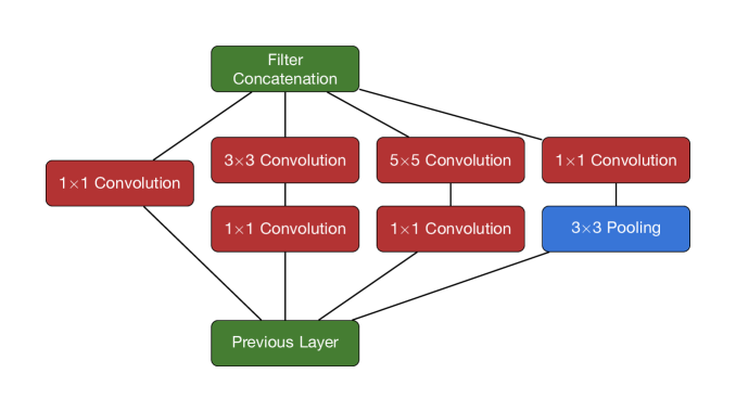
Like any single layer, the inception module takes the set of feature maps produced by the previous layer as input. It then distributes those feature maps to branches, each with filters at different scales. NIN architecture is implemented with $1\times 1$ convolutions to down-sample into a smaller number of maps, maintaining the dimensionality of the input maps. Separate branches perform $3\times 3$ and $5\times 5$ convolution, as well as $3\times 3$ overlapping pooling. The filtered outputs from each branch are then concatenated to produce an output to the next layer with the same number of feature maps, each with the same dimensions, as were passed as input to the inception module.

3 Application to NOvA event classification

We have developed and trained our own CNN, “CVN”, for the identification of neutrino events recorded by the NOvA experiment. NOvA aims to make precision measurements of neutrino oscillation parameters via the disappearance of $\nu_{\mu}$ and appearance of $\nu_{e}$ from neutrino oscillation. NOvA consists of two functionally identical detectors in the NuMI (Neutrinos at the Main Injector) beam [39] at Fermilab which produces a focused beam with an initial flavor composition largely dominated by $\nu_{\mu}$ and a small intrinsic $\overline{\nu}_{\mu}$, $\nu_{e}$, and $\overline{\nu}_{e}$ components. Placing the detectors off-axis at 14.6 mrad provides a narrow-band neutrino energy spectrum near 2 GeV. The Near Detector, located at Fermilab, is placed 1 km from the neutrino source; the Far Detector is located 810 km away near Ash River, Minnesota. The NOvA detectors are composed of extruded PVC cells filled with liquid scintillator which segment the detector into cells with a cross section 3.9 cm wide $\times$ 6.6 cm deep. The cells are 15.5 m long in the Far Detector. Scintillation light from charged particles can be captured by a wavelength shifting fiber which runs through each cell. The end of the fiber is exposed to a single pixel on an avalanche photo-diode array to record the intensity and arrival time of photon signals. The spatial and absolute response of the detector to deposited light is calibrated out using physical standard candles, such that a calibrated response can be derived which is a good estimate of the true deposited energy. Parallel cells are arrayed into planes, which are configured in alternating horizontal and vertical alignments to provide separate, interleaved $X$-$Z$, and $Y$-$Z$ views. The 14,000 ton Far Detector, which is used for the training and evaluation of CVN in this paper, consists of 344,064 total channels arranged into 896 planes each 384 cells wide [6]. Information from the two views can be merged to allow 3D event reconstruction. A schematic of the detector design can be seen in Figure 2.

Figure 2: Schematic of the NOvA detector design

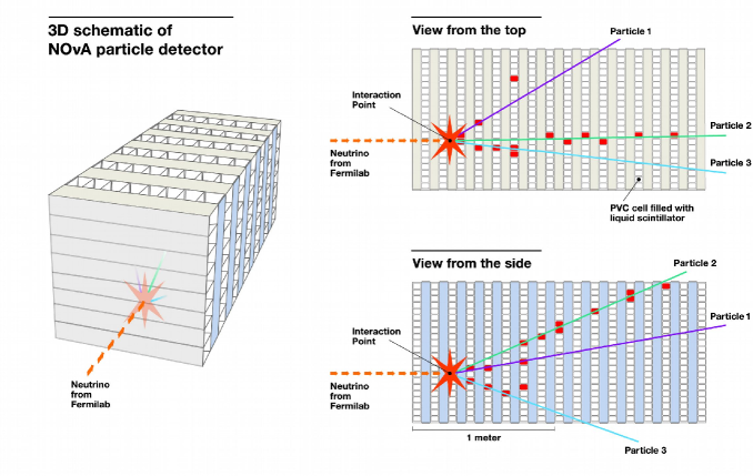
The two figures on the right show the views through the top and side of the three-dimensional figure on the left. They show the ‘hits’ produced as charged particles pass through and deposit energy in the scintillator-filled cells. Illustration courtesy of Fermilab.

Reconstruction of the neutrino energy and flavor state at the detector is essential to neutrino oscillation measurements. The neutrino flavor state can be determined in charged-current (CC) interactions which leave a charged lepton in the final state; an electron in the case of $\nu_{e}$, a muon in the case of $\nu_{\mu}$, or a tau in the case of $\nu_{\tau}$. Neutral-current (NC) interactions bear no signature of the flavor of the interacting neutrino and are thus a background for the charged-current analyses, but may be signal events in other searches.

To support these analyses, we constructed the CVN identifier to characterize candidate neutrino events into one of the following interaction types.

• $\nu_{\mu}$ CC- A muon plus a hadronic component. One of the main topological features of these events is the long, low $dE/dx$ track corresponding to the track of a minimally ionizing muon.

• $\nu_{e}$ CC- An electron plus a hadronic component. The electron topology is typically a wide shower, rather than a track, whose dimensions are related to the radiation length of the detector material.

• $\nu_{\tau}$ CC- A tau plus a hadronic component. The tau is extremely short lived and not visible in the NOvA detector but decays immediately with varying final state probabilities that may produce pions, electrons, muons, and neutrinos. The production threshold for these events is 3.4 GeV, at the upper end of the energy spectrum seen in the NOvA detectors.

• $\nu$ NC- The outgoing lepton in these interactions is a neutrino, which will travel onward undetected. Thus, only the hadronic component of these events is visible, making their flavor impossible to identify.

While it is useful to think about each category as a particular iconic topology, misidentification can still occur. In particular NC interactions can be mistaken for CC interactions when they produce pions which look like leptonic activity. A charged pion track can appear quite similar to a muon track, with the exception of a spike in energy deposition at the end of the track. A neutral pion will rapidly decay to produce a pair of photons which themselves produce electromagnetic showers, which are difficult to distinguish from showers produced by an electron, unless you can find the telltale gap between the interaction vertex and the shower. By constructing an identification algorithm like CVN, which views the entire event topology, we hope to minimize these misidentification failure modes but they remain a challenge.

CC interactions were further divided into quasi-elastic (QE), resonant (RES), and deep-inelastic-scattering (DIS) categories which vary in the complexity of the hadronic portion of the event. QE events are two-bodied with the nucleon recoiling intact from the scattering lepton. In RES events the nucleon is knocked into a baryonic resonance and decays back down to the nucleon with associated hadrons, and in higher energy DIS events the nucleon breaks up in the process of hadronization. Figure 3(c) shows example, simulated, events from these categories as they might be recorded by the NOvA detectors. While the network shows some promise in being able to categorize events at this detailed level, for now we have focused only on neutrino event flavor identification by combining the outputs of these detailed subdivisions into the four categories in the list above.

(a) A $\nu_{e}$ CC QE electron plus one hadron signature where the upward-going shower-like prong with multiple hit cells on each plane corresponds to an electron and the downward-going track-like prong with approximately one hit per plane correspond to a proton.

(b) A $\nu_{e}$ CC RES electron plus hadron shower signature with a characteristic electron shower and short prongs which could correspond to multiple hadrons.

(c) A $\nu_{\mu}$ CC QE muon plus one hadron signature with a long track-like prong with lower charger-per-cell corresponding to a muon and a short prong with larger charge-per-cell corresponding to a proton.

Figure 3: Simulated events in NOvA

Each panel is the side view of a section of the NOvA detector, as depicted in Figure 2. The charge measured in each cell in units of ADC is indicated by color.

The input to CVN was formed first by clustering energy deposits recorded in each scintillator column together in space and time into slices. These slices efficiently separate deposits due to neutrino interactions from those due to cosmic ray interactions and remove nearly all energy deposits due to noise. Grids 100 planes deep and 80 cells wide are chosen which contain the slice. Two separate grids were made for the $x-z$ and $y-z$ detector views. These grids are windows of the detector activity 14.52 m deep and 4.18 m wide. The upstream side of the window was chosen to align with the first plane that contains a detector hit and the window is centered on the median hit cell position. The size and placement of this window ensured that the majority of neutrino events, including muon neutrino CC interactions, are fully contained. The intensity of each pixel in this grid is proportional to the calibrated energy deposition in each scintillator column allowing these projections to naturally be interpreted as grayscale images.

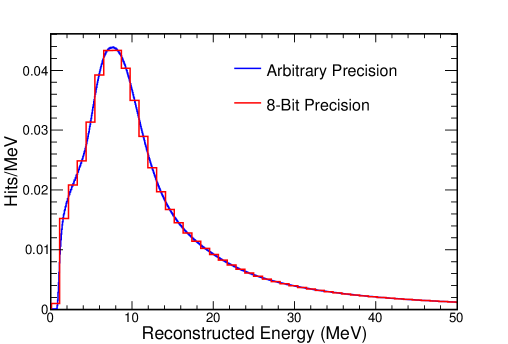
In order to optimize data storage and transfer in the training stage, the pixel intensities were encoded using 8-bits which saturate for hits with energy above 278 MeV. This conversion offers a factor of eight savings over a floating point representation without significantly compromising the representational capacity, as shown in Figure 4. These savings were especially important in reading data from disk into memory during training. This map of 8-bit resolution hits, roughly analogous to an image, was the input to our neural network. Figure 6(c) shows examples of the input to the neural network for three distinct neutrino interaction types.

Figure 4: A comparison of the energy spectrum of individual hits using arbitrarily fine binning and using 256 bins. This shows that it is acceptable to encode pixel intensities using 8-bits. In this encoding, the maximum representable energy per pixel is 278 MeV.

$X$-view

$Y$-view

(a) $\nu_{\mu}$ CC interaction.

$X$-view

$Y$-view

(b) $\nu_{e}$ CC interaction.

$X$-view

$Y$-view

(c) NC interaction.

Figure 6: Example CNN image input

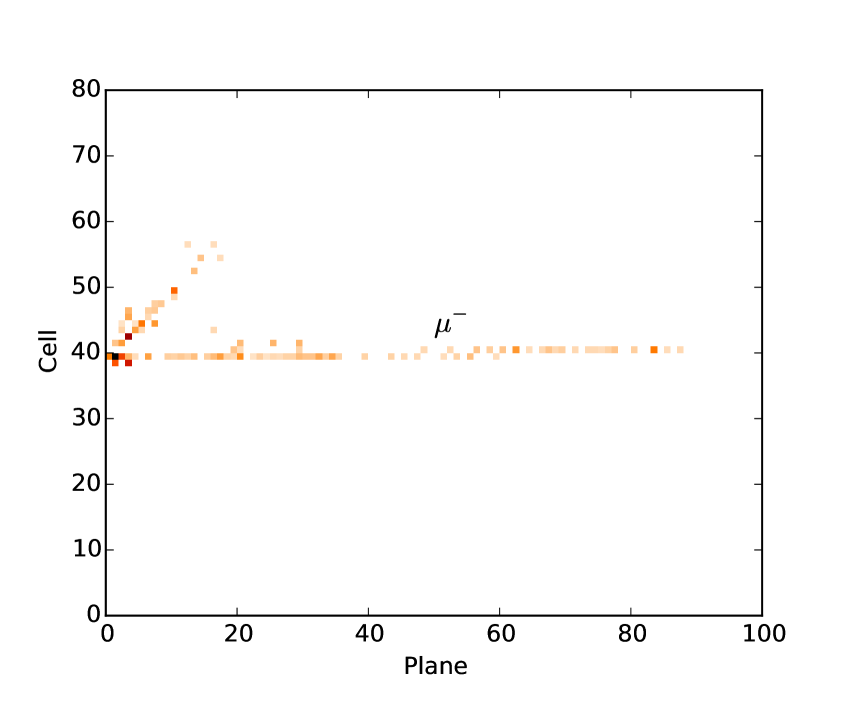
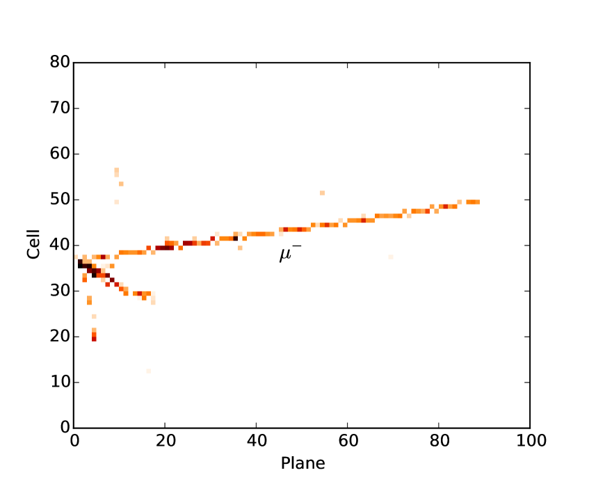
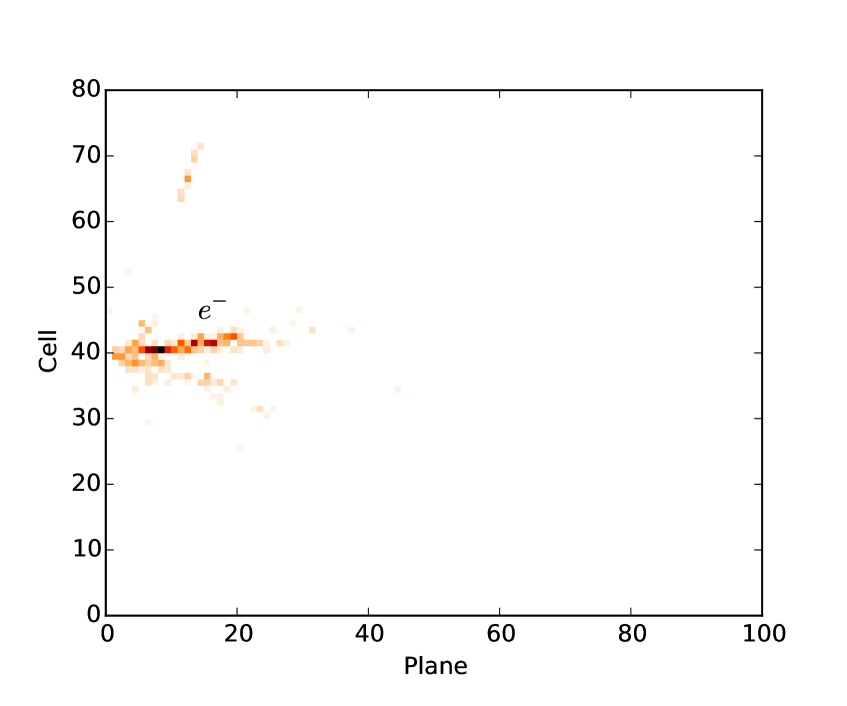
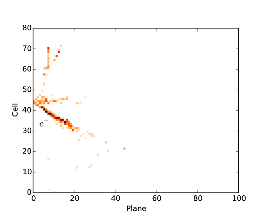
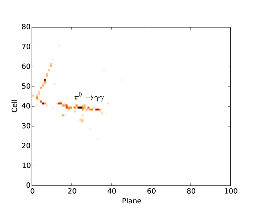
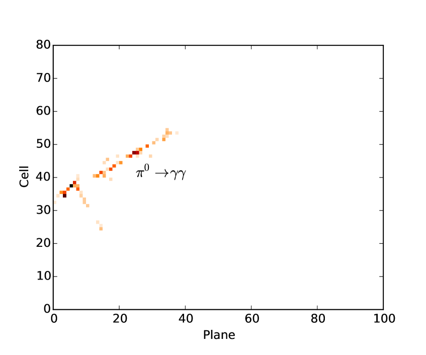
Input given to the CNN for an example $\nu_{\mu}$ CC interaction (top), $\nu_{e}$ CC interaction (middle), and $\nu$ NC interaction (bottom). Hits in the X view of the NOvA detector are shown on the left, and hits in the Y view are shown on the right.

CVN Architecture

Our implementation of CVN was developed using the Caffe [40] framework. Caffe is an open framework for deep learning applications which is highly modular and makes accelerated training on graphics processing units straightforward. Common layer types are pre-implemented in Caffe and can be arranged into new architectures by specifying the desired layers and their connections in a configuration file. Caffe is packaged with a configuration file implementing the GoogLeNet architecture, and we used this as a starting point for designing our own network which is shown in Figure 7.

Figure 7: Diagram of the CNN architecture used for event classification.

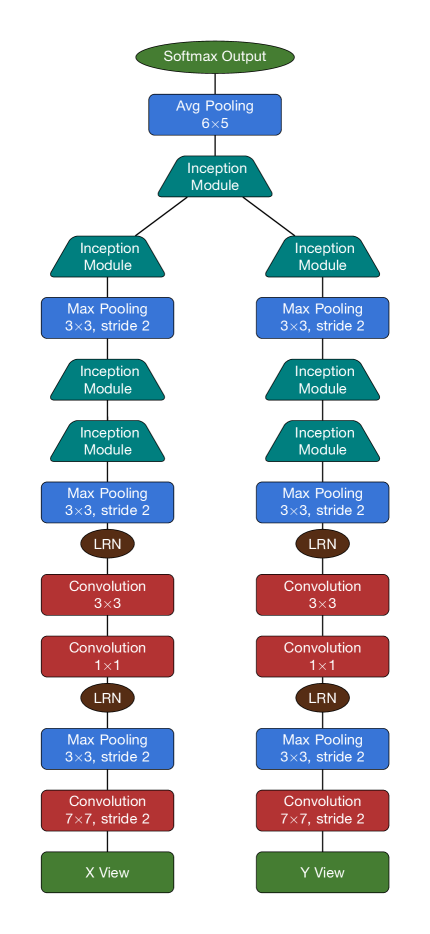
Starting with the input at the bottom, the network has separate branches for the $X$-view and $Y$-view. Each branch undergoes successive convolution, pooling, and local response normalization (LRN). Inception modules are used in downstream layers. The two views are merged and passed through a final inception module, and pooled. The output of the network comes from softmax units.

The CVN architecture differs from the GoogLeNet architecture in a few important ways. First, unlike most natural image problems, we have two distinct views of the same image rather than a single image described in multiple color channels. In order to best extract the information of each view, the channels corresponding to the X and Y-views were split, and each resulting image was sent down a parallel architecture based on GoogLeNet. Since our images are simpler than natural images, it was found that the nine inception modules used in the GoogLeNet network did not improve our results; therefore, we truncated the parallel GoogLeNet networks after three inception modules. At that point, the features from each view were concatenated together and passed through one final inception module to extract combined features. The output of the final inception module was down-sampled using an average pooling layer. During an evaluation (forward) pass, classifier outputs were calculated using the softmax function or normalized exponential function [41] such that the sum of the classifier outputs was always equal to one.

Figure 8: $7\times 7$ convolutional filter and example output

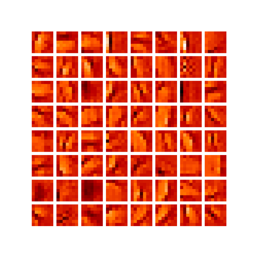
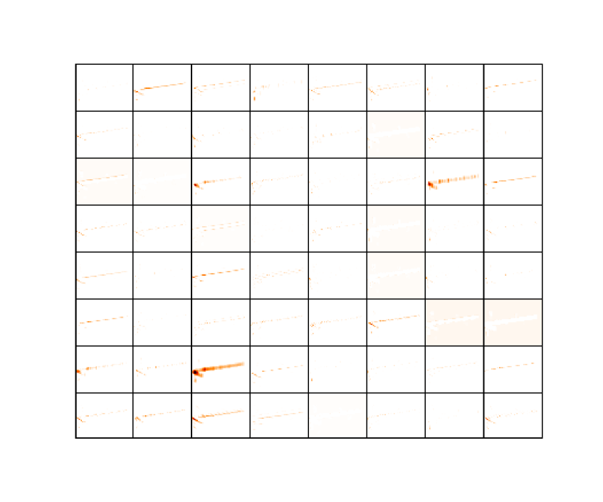
This figure shows the Y view of an example $\nu_{\mu}$ CC interaction (top left), all 64 convolutional filters from the early Y view $7\times 7$ convolutional layer of our trained network (top right), and the output of applying those trained filters to the example event (bottom).

Figure 9: Output of the first inception module

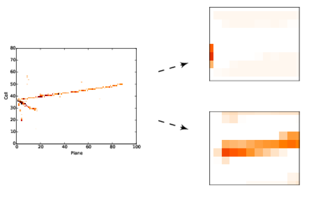
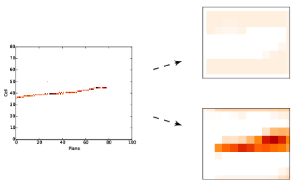
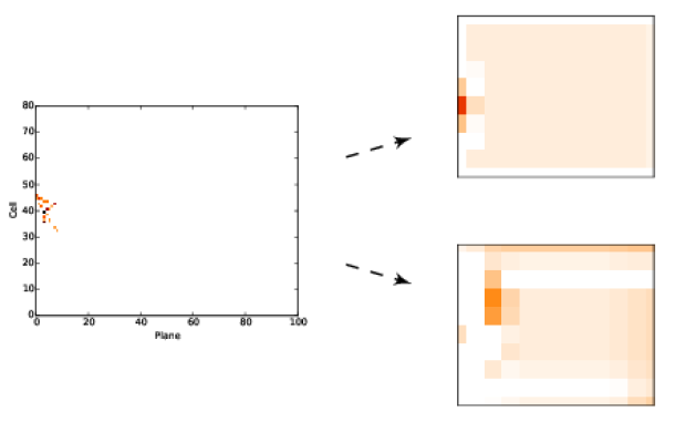
Shown above are three example input images and corresponding example human readable feature maps from the output of the first inception module in the Y view branch of our trained network. Darker regions indicate greater activation, and since this is the output from an early convolutional layer the regions correspond to the regions of the original image. The top-most feature map shows strong responses only in regions where hadronic activity can be found in the original image and the bottom-most feature map shows strong activation only along the path of the muon track. Shown are an example $\nu_{\mu}$ CC DIS interaction (top), $\nu_{\mu}$ CC QE interaction (middle), and $\nu$ NC interaction (bottom).

Training

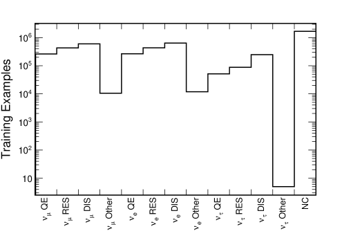
A sample of 4.7 million simulated NOvA Far Detector neutrino events was used as the input to our training, with 80% of the sample used for training and 20% used for testing. FLUKA and FLUGG [42, 43] were used to simulate the flux in the NuMI beamline [44]. Before oscillations, the NuMI beam is composed mostly of $\nu_{\mu}$ with 2.1% intrinsic $\nu_{e}$ contamination. To model $\nu_{e}$ and $\nu_{\tau}$ appearing through oscillation, we perform simulations where the $\nu_{\mu}$ flux has been converted to another flavor. The training sample was composed of one third simulation with the expected, unoscillated flux, one third where the $\nu_{\mu}$ flux was converted to $\nu_{e}$, and one third where the $\nu_{\mu}$ flux was converted to $\nu_{\tau}$. Neutrino-nucleus interactions were simulated using the GENIE [45] package and GEANT4 [46, 47] was used to propagate products of the neutrino interactions through a detailed model of the NOvA detectors. Custom NOvA simulation software converted energy depositions into simulated electronic signals which correspond to the detector output [48]. The only requirements placed on the training events were that they were required to have 15 distinct hits. Distinct categories were created for each GENIE CC interaction mode; $(\nu_{\mu}-{\rm CC},\nu_{e}-{\rm CC},\nu_{\tau}-{\rm CC})\times(QE,RES,DIS,Other)$ and one category was used for all GENIE NC interactions to give the distribution of events by label shown in Figure 10.

Figure 10: Number of events of each category in our training sample

We made use of a Mini-Batch [27] training strategy which simultaneously evaluated 32 training examples in each iteration. During training the final softmax output was used to calculate a multinomial logistic loss [49] by comparing that output to the true target value. We found that we converged to the most optimal versions of CVN by adopting a training strategy whereby the step size of the stochastic gradient descent dropped at fixed intervals. These intervals were chosen to be at points where the network loss improvement rate had plateaued. This strategy, in combination with the vectorized implementation of mini-batch gradient descent within the Caffe framework, allowed for rapid and accurate optimization of our network.

To ensure that a trained model could reasonably generalize beyond the training sample, we employed multiple regularization techniques. We included penalty terms in the back-propagation calculation which are proportional to the square of the weights, thus constraining them to remain small during training. Keeping the weights small prevented the model from responding too strongly to any one input feature. In addition, we applied the dropout technique with $r=0.4$ in the pooling step immediately before the final fully connected layer.

Perhaps the most robust defense against over training is more training data. We augmented our sample using two techniques to add variation to the dataset. First, pixel intensities were varied by adding Gaussian noise with a standard deviation of 1%. Adding noise had the benefit of training the network to rely less heavily on the intensity in each pixel and to adapt to the fluctuations encountered in real data. Second, events were randomly selected to be reflected in the cell dimension, which is roughly transverse to the beam direction. Symmetry in the cell dimension is not perfect; the beam axis is directed $3^{\circ}$ above detector horizon and attenuation in the optical fiber causes thresholding to become more significant for hits further from the readout electronics. However, these effects are small and their presence in fact aids in enhancing variation of the training sample and the robustness of the training against the precise details of the simulation.

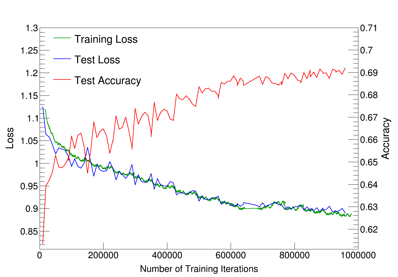
The training of the network presented here was carried out on a pair of NVIDIA Tesla K40s [50] over a full week of GPU hours. Figure 11 shows loss calculated for our training and test samples as a function of number of training iterations; the extremely similar loss on both samples throughout training is a strong indication that the network has not overtrained.

Figure 11: Loss calculated on the training dataset (blue), loss calculated on the test dataset (green), and accuracy calculated on the test dataset (red) as a function of the number of training iterations the network has seen. The training loss shown here is a rolling window average of 40,000 iterations, such that each point represents the average over 128,000 training examples. Each test iteration is the average loss over 256,000 test examples.

4 Results

The same NOvA simulation and software that allowed us to build our training and test samples also allowed us to readily assess the performance of our identification algorithm. To measure performance we used a statistically independent sample of neutrino interactions from that used in the training and testing of CVN. The sample was weighted by the simulated NOvA flux and by neutrino oscillation probabilities from [51] using the NOvA baseline [6] and matter density calculated from the CRUST 2.0 model of the Earth’s crust [52] in order to create a representative mixture of different beam events in the detector. The $\nu_{e}$ selection test uses the preselection described in [53], and the $\nu_{\mu}$ selection uses the preselection described in [54]. These preselections are designed to reject cosmic backgrounds while retaining well-contained neutrino events inside the signal energy window with high efficiency. We quote our selection efficiencies relative to true contained signal, again matching the approach described in  [53] for $\nu_{e}$ and  [54] for $\nu_{\mu}$ tests respectively.

Since the output of the final softmax layer in CVN is normalized to one, it can be loosely interpreted as a probability of the input event falling in each of the thirteen training categories. For the results presented in this paper a $\nu_{e}$ CC classifier was derived from the sum of the four $\nu_{e}$ CC component probabilities. Similarly, the four $\nu_{\mu}$ CC components were summed to yield a $\nu_{\mu}$ CC classification. Figure 12 shows the distribution of the CVN $\nu_{e}$ CC classification parameter for true $\nu_{e}$ CC events from $\nu_{\mu}\rightarrow\nu_{e}$ oscillation and the various NuMI beam backgrounds broken down by type. Figure  13 shows the cumulative efficiency, purity, and their product when selecting all events above a particular CVN $\nu_{e}$ CC classification parameter value. Excellent separation between signal and background is achieved such that the only significant background remaining is that of electron neutrinos present in the beam before oscillation; CVN does not attempt to differentiate between $\nu_{e}$ CC events from $\nu_{\mu}\rightarrow\nu_{e}$ oscillation and those from $\nu_{e}$ which are produced promptly in the neutrino beam; these differ only in their energy distributions. Figures  12 and  13 also show the performance of the CVN $\nu_{\mu}$ CC classification parameter. As with $\nu_{e}$, excellent separation is achieved.

Figure 12: $\nu_{e}$ CC and $\nu_{\mu}$ CC classifier output

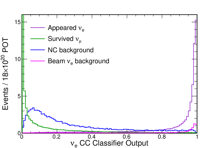
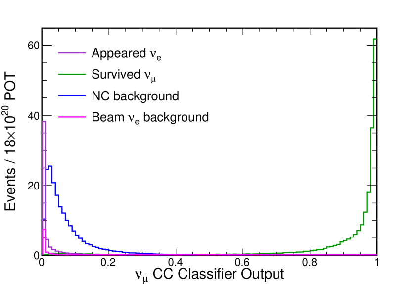
Distribution in $\nu_{e}$ CC Classifier output (top) and $\nu_{\mu}$ CC Classifier output (bottom) for appearing electron neutrino CC interactions (violet), surviving CC muon neutrino (green), NC interactions (blue), and NuMI beam electron neutrino CC interactions (magenta). The y-axis is truncated in the top figure such that the background is not fully visible in order to better show the signal distribution. Distributions are scaled to a NuMI exposure of $18\times 10^{20}$ protons on target, full 14-kton Far Detector.

Figure 13: $\nu_{e}$ CC and $\nu_{\mu}$ CC classifier output performance

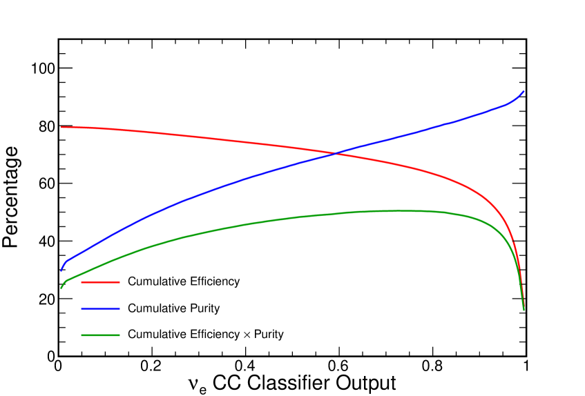
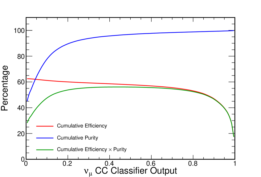
Cumulative efficiency (blue), purity (red), and their product (green) for $\nu_{e}$ CC Classifier output (top) and $\nu_{\mu}$ CC Classifier output (bottom). Efficiency is quoted relative to the true contained signal.

A common way to assess the performance of a signal selection is to compute a Figure of Merit (FOM) given the number of selected signal events $S$ and background events $B$. The FOM $=S/\sqrt{B}$ optimizes for a pure sample useful for establishing the presence of the signal $S$ in the presence of the background, while FOM $=S/\sqrt{S+B}$ optimizes for an efficient sample useful for making parameter measurements with the signal $S$. Table 1 shows the efficiency, purity, and event count at the maximal point for both optimizations when using CVN to select $\nu_{e}$ CC events, and for $\nu_{\mu}$ CC events. Using CVN we were able to set selection criteria well optimized for either FOM when searching for both surviving $\nu_{\mu}$ and appearing $\nu_{e}$ events.

	CVN Selection Value	$\nu_{e}$ sig	Tot bkg	NC	$\nu_{\mu}$ CC	Beam $\nu_{e}$	Signal Efficiency	Purity
Contained Events	$-$	88.4	509.0	344.8	132.1	32.1	$-$	14.8%
$s/\sqrt{b}$ opt	0.94	43.4	6.7	2.1	0.4	4.3	49.1%	86.6%
$s/\sqrt{s+b}$ opt	0.72	58.8	18.6	10.3	2.1	6.1	66.4%	76.0%

(a)

	CVN Selection Value	$\nu_{\mu}$ sig	Tot bkg	NC	Appeared $\nu_{e}$	Beam $\nu_{e}$	Signal Efficiency	Purity
Contained Events	$-$	355.5	1269.8	1099.7	135.7	34.4	$-$	21.9%
$s/\sqrt{b}$ opt	0.99	61.8	0.1	0.1	0.0	0.0	17.4%	99.9%
$s/\sqrt{s+b}$ opt	0.45	206.8	7.6	6.8	0.7	0.1	58.2%	96.4%

(b)

Table 1: Tables showing relative selected event numbers for the various components of the NuMI beam, efficiency, and purity for two different optimizations for the selection of appearing electron neutrino CC interactions (a) and surviving muon neutrino CC interactions (b). Efficiency is shown here relative to the true contained signal. The numbers are scaled to an exposure of $18\times 10^{20}$ protons on target, full 14-kton Far Detector.

Perhaps the most important way to assess the performance of the CVN classification parameters is to compare their performance to the sophisticated identification algorithms already used in recent NOvA publications. For $\nu_{\mu}$ CC interactions the CVN measurement-optimized efficiency of 58% is comparable to the efficiency of 57% quoted in Ref.[54]. This is a modest improvement but shows that CVN algorithm does not underperform when used to identify a class of events we expect to be particularly clear. For $\nu_{e}$ CC interactions the CVN signal-detection-optimized efficiency of 49% is a significant gain over the efficiency of 35% quoted in in Ref.[53]. In both the $\nu_{\mu}$ CC and $\nu_{e}$ CC cases the CVN purity very closely matches the purity of the samples reported in Refs.[54, 53]. The $\nu_{e}$ CC efficiency improvement is significant not just because the $\nu_{e}$ CC signal is particularly hard to separate from its backgrounds, but additionally because the measurements of $\nu_{e}$-appearance and the associated parameters ($\theta_{13}$, neutrino mass hierarchy, etc.) are statistics limited and hence significantly improved by increasing the signal efficiency.

Tests of the CVN selectors response to systematic uncertainties suggest no increased sensitivity to them compared to the the selectors used in Refs.[54, 53]. In particular we studied the variation in signal and background selection for our $\nu_{\mu}$ CC and $\nu_{e}$ CC optimized cuts for a subset of the dominant uncertainties in  Refs.[54, 53], specifically calibration and scintillator saturation uncertainties. For $\nu_{\mu}$ CC interactions the CVN measurement-optimized selection signal sample was sensitive at the $1.9\%$ level, and the extremely small background was sensitive at the $20\%$ level. For $\nu_{e}$ CC interactions the CVN signal-detection-optimized selection signal sample was sensitive at the $1.6\%$ level, and the extremely small background was sensitive at the $1.0\%$ level. In both the $\nu_{\mu}$ CC and $\nu_{e}$ CC cases these shifts are small and comparable to those seen in the selectors used in  Refs.[54, 53].

5 Conclusion and future work

With minimal event reconstruction, we were able to build and train a single algorithm which achieved excellent separation of signal and background for both of the NOvA electron-neutrino appearance and muon-neutrino disappearance oscillation channels. This algorithm, CVN, is a powerful approach to the problem of event classification and represents a novel proof of concept – that CNNs can work extremely well with non-natural images like the readout of a sampling calorimeter. We expect this approach to be transferable to a wide range of detector technologies and analyses.

CVN also opens up other possibilities for event classification and reconstruction which we have just started to explore. For example, the same training and architecture reported here can be expanded to include identification of $\nu$ NC and $\nu_{\tau}$ CC interactions which are used by NOvA in sterile neutrino and exotic physics searches. We also tested the application of CVN to the problem of identification of particles within neutrino events by presenting the algorithm with images of individual, isolated particle clusters [55] along with the images of the overall neutrino event. Initial results have already shown improvements in the efficiency and purity in particle identification over other likelihood methods employed by NOvA and may aid in future cross-section analyses. We are also exploring improvements to cluster-finding and particle identification using semantic segmentation [56] which, starting from the same minimal reconstruction used by CVN, may make it possible to identify the particles which contributed to each “pixel” in the detector readout.

References

- [1] N. S. Altman, An introduction to kernel and nearest-neighbor nonparametric regression, The American Statistician 46 (1992) 175–185, [[http://www.tandfonline.com/doi/pdf/10.1080/00031305.1992.10475879]].
- [2] J. H. Friedman, Stochastic gradient boosting, Computational Statistics & Data Analysis 38 (2002) 367–378.
- [3] F. Rosenblatt, Principles of Neurodynamics: Perceptrons and the Theory of Brain Mechanisms. Spartan Books, 1961.
- [4] R. Reed and R. Marks, Neural Smithing: Supervised Learning in Feedforward Artificial Neural Networks. A Bradford book. MIT Press, 1999.
- [5] Y. LeCun, B. Boser, J. S. Denker, D. Henderson, R. E. Howard, W. Hubbard et al., Backpropagation applied to handwritten zip code recognition, Neural Comput. 1 (Dec., 1989) 541–551.
- [6] NOvA collaboration, D. S. Ayres et al., The NOvA technical design report, FERMILAB-DESIGN-2007-01.
- [7] MINERvA collaboration, L. Aliaga et al., Design, calibration, and performance of the MINERvA detector, Nucl. Instrum. Meth. A 743 (2014) 130 – 159.
- [8] MINOS collaboration, D. G. Michael et al., The magnetized steel and scintillator calorimeters of the MINOS experiment, Nucl. Instrum. Meth. A 596 (2008) 190–228 FERMILAB-PUB-08-126, [[arXiv:0805.3170]].
- [9] A. Bettini et al., The ICARUS liquid argon TPC: A Complete imaging device for particle physics, Nucl. Instrum. Meth. A315 (1992) 223–228.
- [10] H. Chen et al., Proposal for a new experiment using the booster and NuMI neutrino beamlines: MicroBooNE, FERMILAB-PROPOSAL-0974.
- [11] DUNE collaboration, R. Acciarri et al., Long-Baseline Neutrino Facility (LBNF) and Deep Underground Neutrino Experiment (DUNE) Conceptual Design Report Volume 1: The LBNF and DUNE Projects, [arXiv:1601.05471] FERMILAB-DESIGN-2016-01, [[arXiv:1601.05471]].
- [12] DUNE collaboration, R. Acciarri et al., Long-baseline neutrino facility (LBNF) and deep underground neutrino experiment (DUNE) conceptual design report volume 2: The physics program for DUNE at LBNF, [arXiv:1512.06148] FERMILAB-DESIGN-2016-02, [[arXiv:1512.06148]].
- [13] DUNE collaboration, J. Strait et al., Long-baseline neutrino facility (LBNF) and deep underground neutrino experiment (DUNE) conceptual design report volume 3: Long-baseline neutrino facility for DUNE, [arXiv:1601.05823] FERMILAB-DESIGN-2016-03, [[arXiv:1601.05823]].
- [14] DUNE collaboration, R. Acciarri et al., Long-baseline neutrino facility (LBNF) and deep underground neutrino experiment (DUNE) conceptual design report, volume 4 the DUNE detectors at LBNF, [arXiv:1601.02984] FERMILAB-DESIGN-2016-04, [[arXiv:1601.02984]].
- [15] IceCube collaboration, J. Ahrens et al., Sensitivity of the IceCube detector to astrophysical sources of high energy muon neutrinos, Astropart. Phys. 20 (2004) 507–532, [[astro-ph/0305196]].
- [16] IceCube collaboration, R. Abbasi et al., The design and performance of IceCube DeepCore, Astropart. Phys. 35 (2012) 615–624, [[arXiv:1109.6096]].
- [17] S. Fukuda et al., The super-kamiokande detector, Nucl. Instrum. Meth. A 501 (2003) 418 – 462.
- [18] Daya Bay collaboration, X. Guo et al., A Precision measurement of the neutrino mixing angle using reactor antineutrinos at Daya-Bay, [hep-ex/0701029].
- [19] E. Racah, S. Ko, P. Sadowski, W. Bhimji, C. Tull, S.-Y. Oh et al., Revealing Fundamental Physics from the Daya Bay Neutrino Experiment using Deep Neural Networks, [arXiv:1601.07621].
- [20] ATLAS collaboration, G. Aad et al., The ATLAS Experiment at the CERN Large Hadron Collider, JINST 3 (2008) S08003.
- [21] CMS collaboration, S. Chatrchyan et al., The CMS experiment at the CERN LHC, JINST 3 (2008) S08004.
- [22] L. de Oliveira, M. Kagan, L. Mackey, B. Nachman and A. Schwartzman, Jet-Images – Deep Learning Edition, [arXiv:1511.05190].
- [23] K. Hornik, M. Stinchcombe and H. White, Multilayer feedforward networks are universal approximators, Neural Networks 2 (1989) 359 – 366.
- [24] G. Cybenko, Approximation by superposition of a sigmoidal function, Math. Control Signals System 2 (1989) 303–314.
- [25] D. E. Rumelhart, J. L. McClelland and C. PDP Research Group, eds., Parallel Distributed Processing: Explorations in the Microstructure of Cognition, Vol. 1: Foundations. MIT Press, 1986.
- [26] D. E. Rumelhart, G. E. Hinton and R. J. Williams, Learning representations by back-propagating errors, Nature 323 (1986) 533–536+.
- [27] Y. LeCun, L. Bottou, G. B. Orr and K. R. Müller, Neural Networks: Tricks of the Trade. Springer Berlin Heidelberg, 1998.
- [28] Y. Bengio, Learning deep architectures for AI, Foundations and Trends in Machine Learning 2 (2009) 1–127.
- [29] Y. LeCun, Y. Bengio and G. Hinton, Deep learning, Nature 521 (2015) 436–444.
- [30] A. Krizhevsky, I. Sutskever and G. E. Hinton, Imagenet classification with deep convolutional neural networks, in Advances in Neural Information Processing Systems 25, pp. 1097–1105, 2012.
- [31] C. Szegedy, W. Liu, Y. Jia, P. Sermanet, S. Reed, D. Anguelov et al., Going deeper with convolutions, [arXiv:1409.4842].
- [32] C. Farabet, C. Couprie, L. Najman and Y. LeCun, Learning hierarchical features for scene labeling, IEEE Transactions on Pattern Analysis and Machine Intelligence (August, 2013) .
- [33] V. Nair and G. E. Hinton, Rectified linear units improve restricted boltzmann machines, in Proceedings of the 27th International Conference on Machine Learning (ICML-10), pp. 807–814, 2010.
- [34] N. Srivastava, G. Hinton, A. Krizhevsky, I. Sutskever and R. Salakhutdinov, Dropout: A simple way to prevent neural networks from overfitting, Journal of Machine Learning Research 15 (2014) 1929–1958.
- [35] Y. LeCun, K. Kavukcuoglu and C. Farabet, Convolutional networks and applications in vision, in Circuits and Systems (ISCAS), Proceedings of 2010 IEEE International Symposium on, pp. 253–256, 2010. DOI.
- [36] D. Hubel and T. Wiesel, Receptive fields and functional architecture of monkey striate cortex, Journal of Physiology 195 (1968) 215–243.
- [37] O. Russakovsky, J. Deng, H. Su, J. Krause, S. Satheesh, S. Ma et al., ImageNet Large Scale Visual Recognition Challenge, International Journal of Computer Vision (IJCV) 115 (2015) 211–252.
- [38] M. Lin, Q. Chen and S. Yan, Network in network, in International Conference on Learning Representations, 2014. [arXiv:1312.4400].
- [39] K. Anderson et al., The NuMI Facility Technical Design Report, FERMILAB-DESIGN-1998-01.
- [40] Y. Jia, E. Shelhamer, J. Donahue, S. Karayev, J. Long, R. Girshick et al., Caffe: Convolutional architecture for fast feature embedding, [arXiv:1408.5093].
- [41] C. M. Bishop, Pattern Recognition and Machine Learning (Information Science and Statistics). Springer-Verlag New York, Inc., 2006.
- [42] A. Ferrari, P. R. Sala, A. Fassò and J. Ranft, FLUKA: A multi-particle transport code (program version 2005), CERN-2005-010, SLAC-R-773, INFN-TC-05-11.
- [43] T. T. Böhlen, F. Cerutti, M. P. W. Chin, A. Fassò, A. Ferrari, P. G. Ortega et al., The FLUKA code: Developments and challenges for high energy and medical applications, Nuclear Data Sheets 120 (2014) 211 – 214.
- [44] P. Adamson et al., The NuMI Neutrino Beam, Nucl. Instrum. Meth. A806 (2016) 279–306, [[1507.06690]].
- [45] C. Andreopoulos et al., The GENIE neutrino monte carlo generator, Nucl. Instrum. Meth. A614 (2010) 87–104.
- [46] J. Allison et al., Geant4 developments and applications, IEEE Trans. Nucl. Sci. 53 (2006) 270–278.
- [47] S. Agostinelli et al., Geant4 - a simulation toolkit, Nucl. Instrum. Meth. A506 (2003) 250–303.
- [48] A. Aurisano, C. Backhouse, R. Hatcher, N. Mayer, J. Musser, R. Patterson et al., The NOvA simulation chain, J. Phys. Conf. Ser. 664 (2015) 072002 FERMILAB-CONF-15-203-ND.
- [49] J. Long, Regression models for categorical and limited dependent variables. Sage Publ., 1997.
- [50] J. Nickolls, I. Buck, M. Garland and K. Skadron, Scalable parallel programming with cuda, in Que, 2008.
- [51] Particle Data Group collaboration, K. A. Olive et al., Review of particle physics, Chin. Phys. C38 (2014) 090001.
- [52] C. Bassin, G. Laske and G. Masters, The current limits of resolution for surface wave tomography in north america, EOS Trans. AGU 81, F897, 2000.
- [53] P. Adamson et al., First measurement of electron neutrino appearance in NOvA, [arXiv:1601.05022].
- [54] P. Adamson et al., First measurement of muon-neutrino disappearance in NOvA, Phys. Rev. D 93 (2016) 051104.
- [55] M. Baird, J. Bian, M. Messier, E. Niner, D. Rocco and K. Sachdev, Event Reconstruction Techniques in NOvA, J. Phys. Conf. Ser. 664 (2015) 072035.
- [56] J. Long, E. Shelhamer and T. Darrell, Fully convolutional networks for semantic segmentation, in Conference on Computer Vision and Pattern Recognition, 2015. [arXiv:1411.4038].