Blending stiffness and strength disorder can stabilize fracture

Abstract

Quasi-brittle behavior where macroscopic failure is preceded by stable damaging and intensive cracking activity is a desired feature of materials because it makes fracture predictable. Based on a fiber bundle model with global load sharing we show that blending strength and stiffness disorder of material elements leads to the stabilization of fracture, i.e. samples which are brittle when one source of disorder is present, become quasi-brittle as a consequence of blending. We derive a condition of quasi-brittle behavior in terms of the joint distribution of the two sources of disorder. Breaking bursts have a power law size distribution of exponent $5/2$ without any crossover to a lower exponent when the amount of disorder is gradually decreased. The results have practical relevance for the design of materials to increase the safety of constructions.

I Introduction

Disorder is an inherent property of practically all materials, both natural and man made. The heterogeneity occurring on different length scales plays a crucial role in the mechanical response and fracture behavior of materials. On the one hand, the presence of flaws, voids, and grain boundaries reduces the fracture strength, on the other hand, however, they improve the damage tolerance of materials which has a high practical importance for construction components Herrmann and Roux (1990); Alava et al. (2006); Biswas et al. (2015). Low disorder leads to brittle behavior where fracture occurs at a critical load in a catastrophic manner without any precursors. From a practical point of view quasi-brittle behavior is desired, which is typical for materials with a higher amount of disorder. The fracture process of quasi-brittle materials is composed of a large number of intermittent steps of cracking giving rise to the emergence of crackling noise Ramos et al. (2013); Halász et al. (2012). Analyzing the statistics and dynamics of crackling noise, methods can be worked out to forecast the imminent global failure Vasseur et al. (2015). Controlling the amount of disorder to enhance the quasi-brittle behavior of materials has a high practical relevance.

The theoretical investigation of the fracture of heterogeneous materials is mainly based on discrete stochastic models such as Fiber Bundle (FBM) Kun and Herrmann (2000); Hidalgo et al. (2008, 2009); Pradhan et al. (2010), fuse model Nukala et al. (2004) and Discrete Element (DEM) approaches D’Addetta et al. (2002); Carmona et al. (2008); Ergenzinger et al. (2010) with Monte Carlo and molecular dynamics simulation techniques. A common basic assumption of such modeling approaches is that the heterogeneity of materials can be fully captured by introducing disorder for the local fracture strength of cohesive elements of the model. However, recent experimental and theoretical investigations led to the surprising conclusion that the heterogeneity of the local stiffness can improve the fracture toughness of materials Okumura (2004); Urabe and Takesue (2010).

Beyond artificially made (tailored) materials, structural heterogeneity of local stiffness is an important feature of biological materials, as well Okumura and de Gennes (2001); Nukala and Simunovic (2005); Layton and Sastry (2006); Barthelat (2007). One of the most known example of such biological composite materials is nacre which exhibits extraordinary mechanical properties compared to its constituent materials. These features can be partly attributed to the interplay of the local variation of stiffness and strength Okumura and de Gennes (2001); Nukala and Simunovic (2005).

In the present paper we consider this problem in the framework of fiber bundle models (FBM) by introducing two sources of disorder, i.e. both the stiffness and strength of fibers are random variables. Assuming global load sharing after failure events we obtain a generic analytical description of the mechanical response of the system on the macro-level, and investigate the microscopic process of failure by computer simulations. We show that blending stiffness and strength disorder results in stabilization of fracture even if the system with a single source of disorder had a perfectly brittle response.

II Fiber bundle with two random fields

In the model we consider a parallel set of $N$ fibers which is loaded along the fibers’ direction. Fibers have a perfectly brittle response, i.e. they exhibit a linearly elastic behavior with a Young modulus $E$ and fail when the load $\sigma$ on them exceeds a threshold value $\sigma_{th}$. In order to capture the local variation of stiffness and strength of materials, it is a crucial element of the model that each fiber is characterized by two random variables: the Young modulus of fibers $E$ takes values in the interval $E_{-}\leq E\leq E_{+}$ according to the probability distribution $f(E)$, while the breaking threshold $\sigma_{th}$ is sampled with the probability density $g(\sigma_{th})$ over the interval $\sigma_{-}\leq\sigma_{th}\leq\sigma_{+}$. In the present study the two random fields are assumed to be independent, i.e. no correlation is considered between strength and stiffness. Hence, in a finite bundle of $N$ fibers two independent random values $\sigma_{th}^{i}$ and $E_{i}$ are assigned to each fiber $i=1,\ldots,N$. When fibers fail during the stress controlled loading of the bundle the load of broken fibers has to be overtaken by the remaining intact ones. For simplicity, we assume infinite range of load sharing which can be ensured by loading the bundle between two perfectly rigid platens. It has the consequence that the strain $\varepsilon$ of fibers is always the same, however, due to the randomness of the Young modulus $E$ their local load $\sigma_{i}$ is a fluctuating quantity $\sigma_{i}=E_{i}\varepsilon$, where $i=1,\ldots,N$.

In the classical FBM Pradhan et al. (2010); Hidalgo et al. (2009); Yoshioka et al. (2008) the strength of fibers $\sigma_{th}$ is the only random variable which represents the heterogeneity of materials. Since the Young modulus is constant $E=const.$, in the limit of global load sharing of the model fibers keep the same load $E\varepsilon$, and hence, break in the increasing order of their breaking threshold $\sigma_{th}^{i},i=1,\ldots,N$. It has the consequence that the macroscopic constitutive equation $\sigma_{0}(\varepsilon)$ can be expressed in terms of the cummulative distribution of strength thresholds $G(\sigma_{th})=\int_{\sigma_{-}}^{\sigma_{th}}g(x)dx$ in the form

$$\sigma_{0}(\varepsilon)=E\varepsilon\left[1-G(E\varepsilon)\right].$$ (1)

Here the term $\left[1-G(E\varepsilon)\right]$ provides the fraction of intact fibers at the strain $\varepsilon$, and $\sigma_{0}$ denotes the external load.

In the opposite limit of the model all fibers have the same breaking threshold $\sigma_{th}=const.$, however, their Young modulus $E$ is random with $E_{i}$, $i=1,\ldots,N$ values. The breaking condition $E_{i}\varepsilon>\sigma_{th}$ implies that in this case fibers break in the decreasing order of their Young moduli $E_{i}$. Recently, we have shown that in this case the constitutive equation of the model can be obtained as Karpas and Kun (2011)

$${\sigma_{0}(\varepsilon)=\varepsilon\int_{E_{-}}^{\sigma_{th}/\varepsilon}Ef(E)dE,}$$ (2)

where $f(E)$ is the probability density of the Young modulus of fibers. Equation (2) expresses that at a given strain $\varepsilon$ those fibers are intact in the bundle whose stiffness $E$ falls below $\sigma_{th}/\varepsilon$.

Our present fiber bundle model is a combination of the above two cases allowing for randomness both in the stiffness $E$ and strength $\sigma_{th}$ of fibers. In the presence of two disorder fields $E$ and $\sigma_{th}$ the breaking sequence becomes more complex: Fibers break when the load on them $E_{i}\varepsilon$ exceeds the local breaking threshold $E_{i}\varepsilon>\sigma_{th}^{i}$, hence, at a strain $\varepsilon$ those fibers are broken for which the condition $\varepsilon>\sigma_{th}^{i}/E_{i}$ holds. It can be seen that the breaking sequence of fibers is controlled by the ratio of their strength and stiffness which defines their critical strain of breaking $\varepsilon_{th}^{i}=\sigma_{th}^{i}/E_{i}$, and hence, the breaking condition can be formulated as $\varepsilon>\varepsilon_{th}^{i}$. It follows that in our model of random stiffness and strength with global load sharing fibers break in the increasing order of the local failure strain $\varepsilon_{th}^{i}$ ($i=1,\ldots,N$).

Figure 1: Failure plane of fibers for uniformly distributed threshold values. Each point with parameter values ($E,\sigma_{th}$) inside the rectangle of side lengths $E_{+}-E_{-}$ and $\sigma_{+}-\sigma_{-}$ represents a fiber of the bundle. The equation of the dashed straight line is $\sigma_{th}=E\varepsilon$ so that fibers above the line fullfill the condition $\sigma_{th}>E\varepsilon$. At a given strain $\varepsilon$ during the loading process those fibers are intact (highlighted with gray color) and keep the external load, which fall above this line of slope $\varepsilon$. The integral in Eq. (3) has to be performed over the domain of intact fibers.

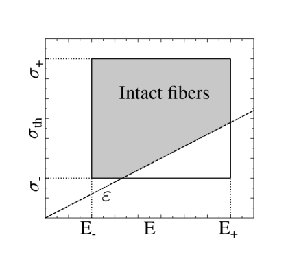
Since the stiffness and the failure strength are independent random variables, the load carried by the intact fibers having Young modulus and strength in the interval $[E,E+dE]$ and $[\sigma_{th},\sigma_{th}+d\sigma_{th}]$, respectively, reads as $E\varepsilon f(E)g(\sigma_{th})dEd\sigma_{th}$. Integrating the contributions of all intact fibers we obtain the generic form of the constitutive equation

$${\sigma_{0}(\varepsilon)=\varepsilon\int_{\sigma_{-}}^{\sigma_{+}}\int_{E_{-}}^{\sigma_{th}/\varepsilon}Ef(E)g(\sigma_{th})dEd\sigma_{th},}$$ (3)

in terms of the probability density functions $f$ and $g$ of the Young modulus and strength of fibers, respectively. First the integral over $E$ has to be performed, where the upper limit $\sigma_{th}/\varepsilon$ of the integral captures the effect that at the macroscopic strain $\varepsilon$ only those fibers can be intact which have a Young modulus below $\sigma_{th}/\varepsilon$ (similarly to Eq. (2)). Then the integral over the strength $\sigma_{th}$ of single fibers follows, where $\sigma_{th}$ can take any value in the range $\sigma_{-}\leq\sigma_{th}\leq\sigma_{+}$.

It can be observed that taking the small strain limit $\varepsilon\rightarrow 0$ in the constitutive equation Eq. (3) we restore linear behavior in the form $\sigma_{0}(\varepsilon\rightarrow 0)=\varepsilon\left<E\right>$ where $\left<E\right>$ denotes the average Young modulus of fibers $\left<E\right>=\int_{E_{-}}^{E_{+}}Ef(E)dE$. In the large strain limit the macroscopic stress goes to zero $\sigma_{0}(\varepsilon\rightarrow\infty)\rightarrow 0$ since there are no intact fibers left. It is important to note that setting the probability distribution of the Young modulus or breaking threshold to a Dirac delta function $f(E)=\delta(E-E_{0})$ and $g(\sigma_{th})=\delta(\sigma_{th}-\sigma_{th}^{0})$, the constitutive equation Eq. (3) of our model recovers the FBM equations Eqs. (1) and (2) with only one source of disorder for failure strength Pradhan et al. (2010); Hidalgo et al. (2009); Yoshioka et al. (2008) and for the Young modulus Karpas and Kun (2011), respectively.

In the following we investigate the breaking process of our FBM both on the macro and micro scales. In order to clarify the effect of blending strength and stiffness disorder we focus on systems which exhibit perfectly brittle failure if only one source of disorder is present.

III Uniformly distributed stiffness and strength

The details of the macroscopic response of the system and of the breaking process of fibers can easily be determined analytically when both the Young modulus $E$ and the strength $\sigma_{th}$ of fibers are uniformly distributed with the probability densities

$${f(E)=\frac{1}{E_{+}-E_{-}},\qquad\mbox{and}\qquad g(\sigma_{th})=\frac{1}{\sigma_{+}-\sigma_{-}}.}$$ (4)

For brevity, we define the notation $\displaystyle{B\equiv f(E)g(\sigma_{th})=1/[(E_{+}-E_{-})(\sigma_{+}-\sigma_{-})]}$, and the strains where the first and last fibers break are denoted by $\varepsilon_{min}\equiv\sigma_{-}/E_{+}$, $\varepsilon_{max}\equiv\sigma_{+}/E_{-}$, respectively. In addition, we introduce $\varepsilon_{1}\equiv\sigma_{-}/E_{-},\ \varepsilon_{2}\equiv\sigma_{+}/E_{+}$ and point out that $\varepsilon_{1}$ can be smaller or larger than $\varepsilon_{2}$ depending on the parameters of the density functions Eq. (4).

III.1 Macroscopic response

The macroscopic constitutive curve $\sigma_{0}(\varepsilon)$ of the bundle can be obtained by inserting the above probability densities Eq. (4) into the generic form Eq. (3). Figure 1 illustrates the failure plane $(\sigma_{th},E)$ where the breaking thresholds $\varepsilon_{th}$ of fibers can take values. When the strain $\varepsilon$ is reached during the loading process those fibers remain intact and keep the load which fall above the straight line of slope $\varepsilon$ (it is highlighted with gray color in the figure).

Figure 2: (Color online) Macroscopic response of a system where both sources of disorder are uniformly distributed with the parameter $W_{E}=0.5$ for three different values of $W_{\sigma}$. Different symbols and colors are used to highlight the regimes corresponding to different terms of the integral expression Eq. (5): bold line (red), circle (blue), square (green), and triangle (magenta) stand for the contributions of the first, second, third, and fourth terms of Eq. (5).

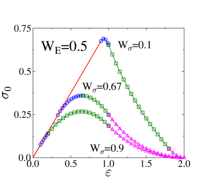
Assuming the case $\varepsilon_{1}<\varepsilon_{2}$ the integrals of Eq. (3) can be carried out in a piecewise manner as

$${\sigma_{0}(\varepsilon)=}\left\{\begin{array}[]{llll}\displaystyle&\displaystyle{0.5(E_{+}+E_{-})\varepsilon},&&\displaystyle{\varepsilon<\varepsilon_{min}};\\[7.11317pt] &\displaystyle{\frac{1}{6B}[-2E_{+}^{3}\varepsilon^{2}-\frac{\sigma_{-}^{3}}{\varepsilon}+3(E_{+}^{2}\sigma_{+}+E_{-}^{2}\sigma_{-}-E_{-}^{2}\sigma_{+})\varepsilon]},&&\displaystyle{\varepsilon_{min}<\varepsilon<\varepsilon_{1}};\\[7.11317pt] &\displaystyle{\frac{1}{6B}[-2(E_{+}^{3}-E_{-}^{3})\varepsilon^{2}+3\sigma_{+}(E_{+}^{2}-E_{-}^{2})\varepsilon]},&&\displaystyle{\varepsilon_{1}<\varepsilon<\varepsilon_{2}};\\[7.11317pt] &\displaystyle{\frac{1}{6B}[2E_{-}^{3}\varepsilon^{2}-3\sigma_{+}E_{-}^{2}\varepsilon+\frac{\sigma_{+}^{3}}{\varepsilon}]},&&\displaystyle{\varepsilon_{2}<\varepsilon<\varepsilon_{max}};\\[8.53581pt] &0,&&\displaystyle{\varepsilon_{max}<\varepsilon}.\end{array}\right.$$ (5)

If $\varepsilon_{2}<\varepsilon_{1}$ the macroscopic behavior is the same except for the interval $\varepsilon_{1}<\varepsilon<\varepsilon_{2}$ (the third interval of Eq. (5)) which is replaced by

$$\sigma_{0}(\varepsilon)=\frac{1}{6B}[-2(\sigma_{+}^{3}-\sigma_{-}^{3})\frac{1}{\varepsilon}-3(\sigma_{+}-\sigma_{-})E_{-}^{2}\varepsilon].$$ (6)

In this case we must also exchange $\varepsilon_{1}$ and $\varepsilon_{2}$ everywhere in the limits of the intervals. In order to quantify the amount of disorder in the system, without loss of generality, from here on end we fix the upper limits $E_{+}=1$ and $\sigma_{+}=1$ and control the disorder by the width of the distributions $W_{E}$ and $W_{\sigma}$ such that $W_{E}\equiv E_{+}-E_{-}$ and $W_{\sigma}\equiv\sigma_{+}-\sigma_{-}$. The macroscopic response $\sigma_{0}(\varepsilon)$ of the fiber bundle is presented in Fig. 2 for several values of $W_{\sigma}$ keeping the width $W_{E}=0.5$ fixed. It can be observed that for strains $\varepsilon<\varepsilon_{\rm min}$, where no fiber breaking occurs, the system exhibits a perfectly linear response with an effective Young modulus equal to the average value $\left<E\right>=(E_{+}+E_{-})/2$ of E. Above $\varepsilon_{\rm min}$ non-linearity emerges as the consequence of gradual breaking of fibers indicating the quasi-brittle behavior of the bundle. Note that the decreasing regime of the constitutive curves in Fig. 2 can only be realized under strain controlled loading conditions. Subjecting the system to an increasing external load catastrophic collapse occurs when the peak of $\sigma_{0}(\varepsilon)$ is surpassed. The value $\sigma_{0}^{c}$ of the peak stress defines the fracture strength of the bundle, while the peak position $\varepsilon_{c}$ provides the critical strain. It can be observed in Fig. 2 that the extension of the non-linear regime preceding macroscopic failure, and hence, the degree of brittleness, strongly depends on the amount of disorder.

III.2 Fraction of broken fibers

In order to quantify the degree of brittleness of the system we determined the fraction of fibers $P_{b}$ which break before the collapse at $\sigma_{0}^{c}$ under stress controlled loading. Perfectly brittle behavior is characterized by the value $P_{b}=0$, since in this case the breaking of the first fiber gives rise to catastrophic failure of the system. Starting from the constitutive equation Eq. (5) we can find the critical strain $\varepsilon_{c}$, and then $P_{b}$ can be obtained from the disorder distribution as

$${P_{b}=1-\int_{\sigma_{-}}^{\sigma_{+}}\int_{E_{-}}^{\sigma_{th}/\varepsilon_{c}}f(E)g(\sigma_{th})dEd\sigma_{th}.}$$ (7)

It has been shown analytically in the classical fiber bundle model, i.e. in the absence of stiffness disorder, that the system has a perfectly brittle response for narrow distributions $W_{\sigma}\leq 0.5$ of fibers’ strength Pradhan et al. (2005); Raischel et al. (2006). Recently, we have demonstrated that in the opposite limit when the uniformly distributed random stiffness is the only source of disorder, the macroscopic response of the bundle is perfectly brittle at any value of $W_{E}$ Karpas and Kun (2011). We evaluated the integral of Eq. (7) by numerical means varying the amount of disorder over the entire range $0\leq W_{E}$, $W_{\sigma}\leq 1$. It can be seen in Fig. 3 that $P_{b}$ obtains a finite value $P_{b}>0$ everywhere in the $W_{E}$ - $W_{\sigma}$ plane except for the $W_{E}$ axis where $W_{\sigma}=0$ holds, and in the range $W_{\sigma}\leq 1/2$ on the $W_{\sigma}$ axis where $W_{E}=0$ holds. The result has the astonishing consequence that whenever there is disorder present both in local strength and stiffness of material elements the macroscopic response of the system is quasi-brittle, i.e. a finite fraction of fibers breaks before the catastrophic failure of the bundle, so that the constitutive curve of the system $\sigma_{0}(\varepsilon)$ is never perfectly linear up to the maximum.

Figure 3: (Color online) The fraction of fibers $P_{b}$ which break before the peak of the constitutive curve is reached during stress controlled loading of the bundle. The surface of $P_{b}(W_{E},W_{\sigma})$ was obtained by numerically evaluating the analytical expression Eq. (7). $P_{b}$ has a finite value everywhere on the $W_{E}$ - $W_{\sigma}$ plane except on the two axis.

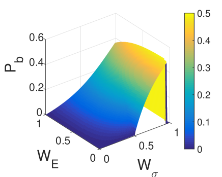
For the case of $W_{E}=0$ the integral of Eq. (7) can be carried out analytically, which yields for the breaking fraction

$$P_{b}(W_{E}=0,W_{\sigma})=\left\{\begin{array}[]{lll}&0&\displaystyle{W_{\sigma}<0.5,}\\[4.2679pt] &\displaystyle{1-\frac{1}{2W_{\sigma}},}&\displaystyle{0.5\leq W_{\sigma}\leq 1}.\end{array}\right.$$ (8)

This result shows that in the absence of stiffness disorder $W_{E}=0$ a transition occurs at $W_{\sigma}=1/2$ between a perfectly brittle $P_{b}=0$ and a quasi-brittle behavior $P_{b}>0$. The numerical results demonstrate that for any finite amount of stiffness disorder $W_{E}>0$ the transition disappears since always a finite fraction of fibers breaks before failure $P_{b}>0$. It follows that blending stiffness and strength disorder can stabilize the system in the sense that no catastrophic collapse can occur without precursors.

IV Condition of stability

In the previous section it has been shown using the cumulative quantity $P_{b}$ that mixing stiffness and strength disorder results in stability of the system in the sense that immediate catastrophic failure at the time of first breaking is avoided. In the following we analyze the transition from the perfectly brittle to quasi-brittle behavior by focusing on the microscopic dynamics of the failure process.

We can formulate a criterion for the stability of the fracture process in terms of the disorder distributions based on the idea that the system is perfectly brittle if the first fiber breaking induces a catastrophic avalanche. At the breaking of the first fiber with the threshold value $\varepsilon_{th}^{min}=\sigma_{-}/E_{+}$ the load on the bundle is $\left<E\right>\varepsilon_{th}^{min}=\left<E\right>\sigma_{-}/E_{+}$. After the breaking event the new Young modulus can be approximated as $\left<E\right>^{\prime}\approx\left<E\right>-E_{+}/N$, which gives rise to a higher strain $\varepsilon^{\prime}$ of the bundle

$$\varepsilon^{\prime}=\frac{\sigma_{-}}{E_{+}}\left[\frac{\left<E\right>}{\left<E\right>-E_{+}/N}\right].$$ (9)

Consequently, the strain increment $\Delta\varepsilon=\varepsilon^{\prime}-\varepsilon_{th}^{min}$ generated by the breaking event under a fixed load can be cast in the form

$$\Delta\varepsilon=\frac{\sigma_{-}}{N\left<E\right>}.$$ (10)

The average number of fiber breakings $a(\varepsilon_{th}^{min})$ induced by the first failure reads as

$$a(\varepsilon_{th}^{min})=Nh(\varepsilon_{th}^{min})\Delta\varepsilon=h\left(\frac{\sigma_{-}}{E_{+}}\right)\frac{\sigma_{-}}{\left<E\right>},$$ (11)

where $h(\varepsilon_{th})$ denotes the probability distribution of threshold strains $\varepsilon_{th}$. The avalanche induced by the first fiber breaking becomes catastrophic if $a(\varepsilon_{th}^{min})>1$, which yields the stability condition of our system

$$h\left(\frac{\sigma_{-}}{E_{+}}\right)\frac{\sigma_{-}}{\left<E\right>}<1.$$ (12)

Note that the condition is general and can be applied to any disorder distribution.

If there is only stiffness disorder present ($\sigma_{th}^{i}=\sigma_{th}$, $i=1,\ldots,N$) the distribution $h(\varepsilon_{th})$ can be obtained from the stiffness distribution $f(E)$ with a simple transformation

$$h(\varepsilon_{th})=f\left(\frac{\sigma_{th}}{\varepsilon_{th}}\right)\frac{\sigma_{th}}{\varepsilon_{th}^{2}}.$$ (13)

Substituting e.g. the uniform distribution Eq. (4) we obtain the condition $E_{+}/(E_{+}-E_{-})<1/\sqrt{2}$, which can never hold. It follows that if the stiffness disorder is the only source of heterogeneity of the system, for uniformly distributed stiffness values the system always has a perfectly brittle behavior. In Ref. Karpas and Kun (2011) the same result was obtained but in a different way focusing on the shape of the constitutive curve.

When both the stiffness and strength of fibers have disorder the probability distribution of the strain thresholds $h(\varepsilon_{th})$ can be calculated as the convolution of $f(E)$ and $g(\sigma_{th})$ taking the ratio of the two random variables $\varepsilon_{th}=\sigma_{th}/E$

$$h(\varepsilon_{th})=\int_{E_{-}}^{E_{+}}Ef(E)g(\varepsilon_{th}E)dE.$$ (14)

We carried out the integration for the specific case when both random variables are uniformly distributed and $\varepsilon_{1}<\varepsilon_{2}$ holds

$$h(\varepsilon_{th})=\left\{\begin{array}[]{lll}0&\displaystyle{\varepsilon_{th}<\frac{\sigma_{-}}{E_{+}},}\\[11.38109pt] \displaystyle{\frac{1}{2B}\left[E_{+}^{2}-\frac{\sigma_{-}^{2}}{\varepsilon_{th}^{2}}\right],}&\displaystyle{\frac{\sigma_{-}}{E_{+}}\leq\varepsilon_{th}<\frac{\sigma_{-}}{E_{-}},}\\[11.38109pt] \displaystyle{\frac{1}{2B}\left[E_{+}^{2}-E_{-}^{2}\right],}&\displaystyle{\frac{\sigma_{-}}{E_{-}}\leq\varepsilon_{th}<\frac{\sigma_{+}}{E_{+}},}\\[11.38109pt] \displaystyle{\frac{1}{2B}\left[\frac{\sigma_{+}^{2}}{\varepsilon_{th}^{2}}-E_{-}^{2}\right],}&\displaystyle{\frac{\sigma_{+}}{E_{+}}\leq\varepsilon_{th}<\frac{\sigma_{+}}{E_{-}},}\\[11.38109pt] 0&\displaystyle{\varepsilon_{th}>\frac{\sigma_{+}}{E_{-}}.}\end{array}\right.$$ (20)

Figure 4: (Color online) Probability distribution $h(\varepsilon_{th})$ of the strain thresholds $\varepsilon_{th}$ of fibers calculated from Eq. (20) for three parameter sets.

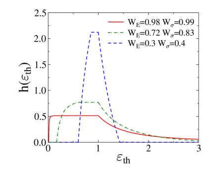
Figure 4 illustrates the distribution $h(\varepsilon_{th})$ for three combinations of $W_{E}$ and $W_{\sigma}$. It can be observed that for uniformly distributed stiffness and strength the distribution of the strain thresholds $h(\varepsilon_{th})$ starts continuously from zero for any finite value of $\sigma_{-}$ without any finite jump. This feature explains why the combination of two perfectly brittle systems leads to the emergence of quasi-brittle behavior where stable cracking precedes macroscopic failure. For the case $\sigma_{-}=0$ the distribution starts with a finite constant, however, the small strain value $\varepsilon\simeq 0$ still ensures stability. For those disorder distributions of stiffness and strength which cover the range from 0 to $+\infty$ stability of the blend is again guaranteed by the generic form of the distribution Eq. (14).

V Avalanches of fiber failures

Under quasi-statically increasing external load $\sigma_{0}$ when a fiber breaks its load gets redistributed over the remaining intact fibers which may induce further failure events. As a consequence of subsequent load redistribution a single breaking fiber may trigger an entire avalanche of breaking events. The randomness of local physical properties and the interaction of fibers introduced by the load sharing result in highly complex microscopic dynamics of the failure process Kloster et al. (1997); Hidalgo et al. (2009). In the following we explore the statistics of breaking avalanches of fibers by computer simulations.

V.1 Computer simulation technique

First we present the algorithm which allows us to simulate the fracture process of large bundles. It has been assumed that the bundle is loaded between stiff platens which ensures that the strain of fibers is the same $\varepsilon$. As the external load $\sigma_{0}$ is increased the fibers break in the increasing order of their failure strain $\varepsilon^{i}_{th}$, determined as $\varepsilon^{i}_{th}=\sigma^{i}_{th}/E^{i}$ ($i=1,\ldots,N$) which fall in the range $\sigma_{-}/E_{+}\leq\varepsilon_{th}\leq\sigma_{+}/E_{-}$. Computer simulation of the failure process of a finite bundle of $N$ fibers under stress controlled loading proceeds in the following steps:

1. Generate random values of the Young modulus $E_{i}$, and failure strength $\sigma_{th}^{i}$, $i=1,\ldots,N$ of fibers according to the desired distributions $f(E)$ and $g(\sigma_{th})$. Independence of the random fields has to be ensured.

2. Determine the failure strains $\varepsilon_{th}^{i}=\sigma_{th}^{i}/E_{i}$, $i=1,\ldots,N$, and sort them into ascending order.

3. Increase the externally imposed strain $\varepsilon$ up to the smallest threshold $\varepsilon=\varepsilon_{th}^{min}$, and remove the breaking fiber. At this instant there is $\sigma_{0}=\left<E\right>\varepsilon$ load on the system, where the initial value of the average Young modulus of the bundle reads as

   $$\left<E\right>=\frac{1}{N}\sum_{i=1}^{N}E_{i}.$$ (21)

4. After the breaking event the load of the broken fiber gets redistributed over the remaining intact ones keeping the external load $\sigma_{0}$ constant. This load redistribution may induce additional fiber failures and eventually can even trigger an avalanche of breaking events. Note that due to the random stiffness, fibers keep a different amount of load that is why long range interaction is easier to realize through the control of strain. Triggered breakings can be determined in the following way: after the breaking event the overall Young modulus of the bundle has to be updated

   $$\left<E\right>^{\prime}=\frac{1}{N_{int}}\sum_{i\in I}E_{i},$$ (22)

   where $I$ denotes the set of intact fibers which has $N_{int}$ elements.

   Since $\left<E\right>^{\prime}<\left<E\right>$ and the external load is kept constant, the strain of the bundle increases to the new value $\varepsilon^{\prime}$, which can be obtained as

   $$\varepsilon^{\prime}=\left<E\right>\varepsilon/\left<E\right>^{\prime}.$$ (23)

5. Those fibers which have threshold values below the the updated strain $\varepsilon_{th}^{j}<\varepsilon^{\prime}$ have to be removed and the algorithm is continued with step 4. During bursts of breaking one has to take into account in Eq. (22) that more than one fiber may also break in an iteration step.

6. If no more fibers break due to load redistribution, the avalanche ended and the external strain can be increased again to the strain threshold of the next intact fiber in the sorted sequence of $\varepsilon_{th}$.

The efficiency of the algorithm enabled us to simulate bundles of $N=10^{7}$ fibers averaging over 5000 samples at each parameter set with moderate CPU times.

V.2 Size distribution of bursts

Using the above algorithm we explored the bursting activity accompanying the stress controlled loading process of quasi-brittle systems with two sources of disorder. The avalanches are characterized by their size $\Delta$, which is defined as the number of fibers breaking in the correlated trail of the avalanche. For the classical FBM, where the fiber strength is the only source of disorder, it has been shown analytically Kloster et al. (1997); Pradhan et al. (2010); Hidalgo et al. (2009) and by computer simulations Hidalgo et al. (2009); Kun et al. (2000) that for equal load sharing the size distribution of avalanches $p(\Delta)$ has a power law behavior

$$p(\Delta)\sim\Delta^{-\tau}.$$ (24)

The value of the exponent $\tau=5/2$ is universal for a broad class of failure threshold distributions Kloster et al. (1997); Pradhan et al. (2010); Hidalgo et al. (2009).

Figure 5: (Color online) Burst size distributions $p(\Delta)$ for several values of strength disorder $W_{\sigma}$ in the absence of stiffness disorder $W_{E}=0$. Approaching the brittle regime $W_{\sigma}\to 1/2$ the well known result of the crossover in $\tau$ from $5/2$ to $3/2$ is recovered. The two straight lines represent power laws with exponents $3/2$ and $5/2$. The inset presents the constitutive behaviour of the system for three values of $W_{\sigma}$.

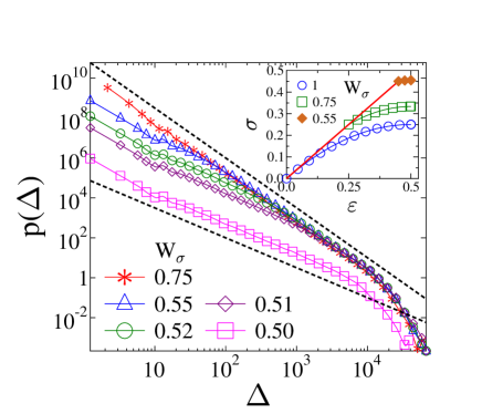
Avalanches occur until the disorder is high enough in the system $W_{\sigma}>\sigma_{+}/2$ Pradhan et al. (2005); Raischel et al. (2006). In the limiting case $W_{\sigma}\rightarrow\sigma_{+}/2$ the quasi-brittle region where avalanche precursors occur, shrinks such that when $W_{\sigma}\leq\sigma_{+}/2$ the response of the bundle becomes perfectly brittle and the system collapses without having any finite size avalanches. The constitutive behaviour of the system under stress controlled loading is shown in the inset of Fig. 5 for a few values of $W_{\sigma}$, where the shrinking of the quasi-brittle regime can be observed. Approaching the brittle limit the power law size distribution of avalanches prevails, however, $p(\Delta)$ exhibits a crossover to a lower exponent $\tau=3/2$ in agreement with previous findings Hidalgo et al. (2009); Pradhan et al. (2005); Raischel et al. (2006). This behavior can be seen in Fig. 5 where avalanche size distributions $p(\Delta)$ of our model are presented for several values of $W_{\sigma}$ at zero stiffness disorder $W_{E}=0$. Approaching the brittle limit the lower value of the avalanche size exponent $\tau=3/2$ means that the fraction of large size events gets higher since the breaking of stronger fibers can trigger more secondary breakings. Avalanches of breaking fibers are analogous to acoustic outbreaks generated by the nucleation and propagation of cracks in heterogeneous solids under an increasing stress Niccolini et al. (2011); Salminen et al. (2002); Diodati et al. (1991). Recording the acoustic waves that emanate from the material is an indicator of the breaking phenomena on the microscopic level. It has been addressed that the crossover in $\tau$ could be exploited to forecast the imminent catastrophic failure Pradhan and Chakrabarti (2002); Pradhan et al. (2005).

In Sec. III.1 the analysis of the fraction of broken fibers $P_{b}$ at the peak load has already shown that adding a second source of disorder to an otherwise brittle system, quasi-brittle behavior emerges, i.e. $P_{b}$ is never zero when $W_{\sigma},W_{E}>0$. It has the interesting consequence that macroscopic failure is always preceded by finite avalanches which behave as precursors to failure. To demonstrate this effect in Fig. 6$(a)$ avalanche size distributions are presented for $W_{\sigma}=0.25$ which should provide perfectly brittle behavior (no stable avalanches) if strength is the only source of disorder. Simulations revealed that for any finite value of $W_{E}$ the size distribution $p(\Delta)$ has a power law behavior as in Eq. (24) followed by a stretched exponential cutoff. For the value of the power law exponent the usual mean field value $\tau=5/2$ was obtained. It can be observed that the amount of disorder $W_{E}$ only controls the total number of avalanches and the cutoff burst size of the distributions. Figure 6$(b)$ shows that rescaling the burst size by the $\alpha=1/2$ power of $W_{E}$ all the distributions can be collapsed on a master curve. This high quality scaling collapse demonstrates that the exponent $\tau$ is independent of the amount disorder, even in the limit of very low $W_{E}$ the same exponent $\tau=5/2$ is retained. Note that due to the normalization of the distributions along the vertical axis scaling is done with the product of the two exponents $\alpha$ and $\tau$.

We have pointed out in Ref. Karpas and Kun (2011) that when stiffness is the only source of disorder $W_{\sigma}=0$ perfectly brittle behavior occurs for any value of $W_{E}$. However, in the present study we have shown that adding strength disorder leads to stabilization. Avalanche size distributions are presented in Fig. 6$(c)$ for $W_{E}=1$ varying the amount of strength disorder in a broad range. Again the same functional form occurs as in Fig. 6$(a)$ with the same exponent $\tau=5/2$ for all the parameter sets. The scaling collapse in Fig. 6$(d)$ is also obtained with the exponent $\alpha=1/2$ as for the case of varying stiffness disorder. The data collapse analysis also implies that the cutoff burst size $\Delta_{c}$ of the distributions has a power law dependence on the amount of disorder in the form $\Delta_{c}\sim W_{E}^{\alpha}$ and $\Delta_{c}\sim W_{\sigma}^{\alpha}$ when the stiffness and strength disorder are varied, respectively, in the limit of low disorder.

A very important consequence of the above numerical analysis is that when approaching the brittle limit $W_{E}\to 0$ for $W_{\sigma}<1/2$ and $W_{\sigma}\to 0$ for $W_{E}>0$, the avalanche size distributions do not show any crossover to a lower exponent. Reducing the amount of disorder both the number and size of avalanches decreases, however, the value of the power law exponent $\tau$ remains robust. Crossover occurs when solely strength disorder is present $W_{E}=0$.

Figure 6: (Color online) $(a)$ Size distribution of bursts for $W_{\sigma}=0.25$ varying the stiffness disorder $W_{E}$ in a broad range. $(b)$ Scaling collapse of the distributions of $(a)$. Best collapse is achieved with the exponent $\alpha=1/2$. In $(a)$ and $(b)$ the same legend is used. $(c)$ Size distribution of bursts for $W_{E}=1$ varying the amount of strength disorder $W_{\sigma}$ in a broad range. $(d)$ Scaling collapse of the distributions of $(c)$ using the exponent $\alpha=1/2$. In $(c)$ and $(d)$ the same legend is used.

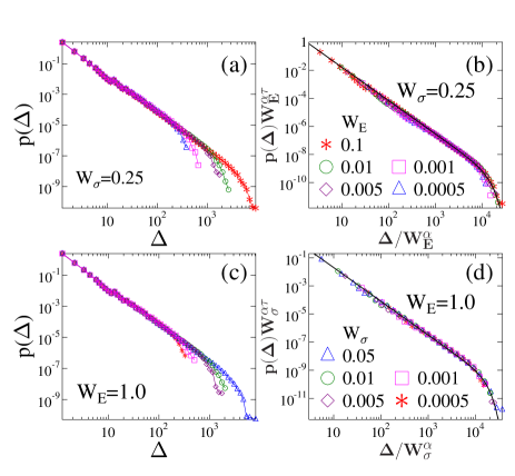
Note that no similar scaling behaviour can be observed when only one source of disorder is present: For constant fiber strength, the system has a perfectly brittle behaviour at any values of $W_{E}$. When strength is the only source of disorder the bundle becomes critical already when $W_{\sigma}$ approaches $1/2$. It has the consequence that in the limit $W_{\sigma}\to 1/2$ the characteristic avalanche size increases, i.e. just the opposite happens to what we have presented above. When the two disorders are blended the reason of the decreasing avalanche activity is that for any $W_{E}$ and $W_{\sigma}$ the threshold distribution $h(\varepsilon_{th})$ starts from a zero value even if the thresholds have a finite lower bound $\varepsilon_{th}^{min}>0$.

VI Discussion

The fracture of disordered materials proceeds in bursts which can be recorded in the form of acoustic noise. Measuring crackling noise is the primary source of information about the microscopic dynamics and time evolution of fracture. From laboratory experiments through engineering constructions to the scale of natural catastrophes forecasting techniques of imminent global failure strongly rely on identifying signatures in the evolving temporal sequence of breaking bursts Sammonds et al. (1992); Stojanova et al. (2014). When the disorder is absent or its amount is not sufficiently high, failure occurs in a catastrophic manner without any precursors. Hence, enhancing the quasi-brittle nature of fracture by controlling disorder is of high practical importance.

In the present paper we considered this problem in the framework of fiber bundle models. This approach provides a simple representation of the disorder and allows for the investigation of the microscopic dynamics of the failure process under various types of loading conditions. The classical setup of FBMs assumes constant Young modulus of fibers so that the heterogeneous microstructure is solely captured by the random strength of fibers. Here we proposed an extension of FBMs by considering simultaneously two sources of disorder, i.e. both the strength and stiffness of fibers are random variables independent of each other. We carried out a detailed analytical and numerical investigation of the fracture process of the system under quasi-statically increasing external load both on the macro and micro scales.

For the case of global load sharing we showed that introducing a second source of disorder stabilizes the system in the sense that a bundle which has a perfectly brittle behavior becomes quasi-brittle whenever a finite amount of disorder of the other field is added. We gave a general analytical derivation of the constitutive equation and of the stability criterion of the system in terms of the disorder distributions. For the purpose of numerical investigations an efficient simulation technique was worked out. As a specific case we considered uniformly distributed strength and stiffness of fibers controlling the amount of disorder by the width of the distributions. Investigating the microscopic process of failure we pointed out that the size of crackling bursts is power law distributed followed by an exponential cutoff. The power law exponent proved to be equal to the usual mean field exponent $5/2$ without having any crossover to a lower value when approaching the limit of perfect brittleness. The amount of disorder only controls the number of avalanches and their cutoff size. The origin of the stabilization mechanism is that the distribution of the relevant failure threshold, obtained as the convolution of the stiffness and strength distributions of fibers, starts from a zero value even if the thresholds have a finite lower bound.

Recently, the problem of mixing strength and stiffness disorder has been considered in a simplified modelling framework: in Ref. Roy and Goswami (2015) a bundle was composed of a few groups of fibers of different Young moduli having uniformly distributed failure strength. Approximate calculations showed that increasing the number of groups of equally spaced Young modulus values the bundle retains the quasi-brittle behaviour for narrower strength distributions. Our analytical results provide a general understanding of the findings of Ref. Roy and Goswami (2015) with the additional outcome that the continuous stiffness distribution of our study corresponds to an infinite number of groups of fibers where stability is ensured for any finite amount of strength disorder.

To test the generality of our results, we also considered the case where the breaking threshold and Young modulus of fibers follow a Weibull distribution with a lower cutoff $x_{-}$. Here $x$ stands for both strength $\sigma_{th}$ and stiffness $E$. Simulations performed with several values of $x_{-}$ verified that any finite amount of disorder leads to quasi-brittle behavior of the bundle when two sources of disorder are present. Furthermore, the burst size distribution exponent $\tau$ displayed a crossover from $5/2$ to $3/2$ only when the strength disorder was reduced in the absence of stiffness disorder in agreement with Pradhan et al. (2006).

Besides their theoretical importance our results have practical relevance for materials’ design, the controlled blending of stiffness and strength disorder is a promissing way to increase the safety of constructions. Most of our results are formulated in a general way so that they can be applied to any strength and stiffness distributions used in engineering and materials science. Biological materials exhibit a broader variety of stiffness and strength than engineering materials which could also be captured in the framework of our model. An important limitation of our study that has to be resolved is the assumption that thrength and stiffness of material elements are uncorrelated. In real materials correlations naturally develop such that higher stiffness may be accompanied by higher strength. Work is in progress to capture these types of correlation in our model.