How Density Environment Changes the Influence of the Dark Matter-Baryon Streaming Velocity on the Cosmological Structure Formation
Abstract
We study the dynamical effect of relative velocities between dark matter and baryonic fluids, which remained supersonic after the epoch of recombination. The impact of this supersonic motion on the formation of cosmological structures was first formulated by Tseliakhovich & Hirata (2010), in terms of the linear theory of small-scale fluctuations coupled to large-scale, relative velocities in mean-density regions. In their formalism, they limited the large-scale density environment to be those of the global mean density. We improve on their formulation by allowing variation in the density environment as well as the relative velocities. This leads to a new type of coupling between large-scale and small-scale modes. We find that the small-scale fluctuation grows in a biased way: faster in the overdense environment and slower in the underdense environment. We also find that the net effect on the global power spectrum of the density fluctuation is to boost its overall amplitude from the prediction by Tseliakhovich & Hirata (2010). Correspondingly, the conditional mass function of cosmological halos and the halo bias parameter are both affected in a similar way. The discrepancy between our prediction and that by Tseliakhovich & Hirata (2010) is significant, and therefore the related cosmology and high-redshift astrophysics should be revisited. The mathematical formalism of this study can be used for generating cosmological initial conditions of small-scale perturbations in generic, overdense (underdense) background patches.
1 Introduction
The -cold dark matter (CDM) scenario, combined with the theory of cosmic inflation, is the successful, concurrent model describing the past and the present of our universe, consistent with a wide range of observations. In this scenario, cosmological structures grow out of an extremely uniform density field but with tiny fluctuations that are seeded by the cosmic inflation. The growth of the CDM density fluctuations and the growth of baryon density fluctuations are not in perfect synchronization, because baryons were tightly coupled to photons before the epoch of recombination and thus their motion was different from the motion of CDM which only reacts to gravity. Only after recombination baryons gradually decoupled from photons, and followed the motion of the CDM under gravity.
Cosmological observations have verified the CDM scenario in scales large enough to make the baryonic physics almost irrelevant (e.g. Komatsu et al. 2011; Reichardt et al. 2012 Planck Collaboration et al. 2015). However, once in the regime where the baryonic physics becomes important, the growth of baryon fluctuations is affected by hydrodynamics and the growth of the CDM is affected by the gravitational feedback from the baryon fluctuations. Some of the usual assumptions that are made for treating very large scales, therefore, should be taken carefully or modified when treating relatively small scales. For example, Naoz & Barkana (2005) improved on the previous estimation of the linear density power spectrum in small scales, by replacing the usual assumption made in cosmology that the sound speed of baryons is uniform in space with the fact that the sound speed fluctuates in space in small scales. They showed that more than change occurs in the baryon density power spectrum and even more change in the baryon temperature power spectrum. A sheer inclusion of the sub-dominant, yet non-negligible baryonic component in the analysis changes the prediction on the matter density power spectrum at a few percent level even in large scales, as was shown in the framework of the high-order perturbation theory (Shoji & Komatsu, 2009; Somogyi & Smith, 2010).
Similarly, the relative velocity (“streaming velocity”) between baryons and the CDM after the recombination should also be considered carefully in cosmology. Tseliakhovich & Hirata (2010, TH hereafter), for the first time, properly calculated the growth of small-scale density fluctuations under the influence of the streaming velocity. Small-scale fluctuations are coupled to large-scale streaming velocity fields which are coherent over a few comoving Mpc scale. This has its own spatial fluctuation with km/s standard deviation at the epoch of recombination, and then decays in proportion to the inverse of the scale factor . Its impact on the small-scale structure formation is non-negligible because the streaming velocity remains supersonic (until the intergalactic medium is strongly heated). This then leads to the suppression of small-scale matter density fluctuations. The wave-modes that are the most strongly affected are around Mpc, and the impact is on the matter power spectrum, the conditional mass function and the halo bias parameter, to name a few (TH).
Subsequent studies have considered the impact of the streaming velocity in the perspective of both cosmology and astrophysics. The boost of amplitude and the shift of the peak of the baryonic acoustic oscillation (BAO) feature due to the streaming velocity, in the gas intensity mapping or the galaxy survey, were intensively investigated (Dalal et al. 2010; Yoo et al. 2011; McQuinn & O’Leary 2012; Slepian & Eisenstein 2015; Lewandowski et al. 2015; Blazek et al. 2015; Schmidt 2016). They find that both high-redshift (e.g. Dalal et al. 2010; McQuinn & O’Leary 2012) and low-redshift (e.g. Yoo et al. 2011) surveys will be affected. The impact of the streaming velocity on BAO may be separated out from the impact of the matter density itself (Slepian & Eisenstein 2015), which is important because otherwise it will become another nuisance parameter in cosmology. The astrophysical impact of the streaming velocity has been investigated with focus on the formation of the nonlinear structure such as cosmological halos and stellar objects (Maio et al. 2011; Stacy et al. 2011; Greif et al. 2011; Tseliakhovich et al. 2011; Naoz et al. 2012; Fialkov et al. 2012; O’Leary & McQuinn 2012; Bovy & Dvorkin 2013; Richardson et al. 2013; Tanaka et al. 2013; Naoz & Narayan 2014; Popa et al. 2015; Asaba et al. 2016). Most studies indicate that the formation of minihalos (roughly in the mass range ) and the formation of stellar objects in them are suppressed. It may induce baryon-dominated objects such as globular clusters (Naoz & Narayan 2014; Popa et al. 2015), but the actual star formation process leading to globular clusters has yet to be simulated. It may be responsible even for the generation of the primordial magnetic field (Naoz & Narayan 2013). Because minihalos are the most strongly affected among cosmological halos and they are responsible for the early phase of the cosmic reionization process, how they change the high-redshift 21-cm background is also of a prime interest (Visbal et al. 2012; McQuinn & O’Leary 2012; Fialkov et al. 2013). It is noteworthy that some of these numerical simulation results (Maio et al. 2011; Stacy et al. 2011; Greif et al. 2011), which are based on the initial condition generated by the usual Boltzmann solver such as the Code for Anisotropies in the Microwave Background (CAMB: Lewis et al. 2000), need to be re-examined. This is because the impact of the streaming velocity is cumulative and inherent even at (McQuinn & O’Leary 2012), at which or later these simulations start with a streaming velocity implemented by hand.
The original formalism by TH has been re-investigated in terms of the high-order perturbation theory in the wave-number space (“-space” henceforth), and some “missing terms” previously neglected were found important (Blazek et al. 2015; Schmidt 2016). Basically, for the large-scale modes responsible for the streaming velocity (), TH used a trivial solution for the evolution of the streaming velocity () and the density ( and being overdensities of the CDM and baryons in large scale, respectively) environment: , . Treating this as a new 0th-order solution to the perturbation equations, they then examined how the perturbation in small scales grows. In doing so, they treated as a spatial quantity and perturbation variables in small scales as -space quantities. This is basically a high-order perturbation theory, coupling large-scale mode () and the small-scale modes ( and , small scale CDM and baryonic overdensities, respectively). However, is tightly linked to the fluctuating and through the density continuity equation, and thus the trivial solution adopted by TH cannot be used for generically overdense and underdense regions. The continuity equation connects the divergence of to and , and Schmidt (2016) finds that the divergence of is indeed an important term that one should not ignore. Blazek et al. (2015) also works on the generic basis of non-zero and .
We improve on the formalism of TH by also considering the non-zero overdensities. Toward this end, different from Blazek et al. (2015) and Schmidt (2016), we inherit the original method by TH and focus on the impact on small-scale modes: large-scale is treated as the spatial quantity and small-scale overdensities and are treated as the -space quantity in the perturbation analysis. Most importantly, we explicitly include generically “non-zero” and as a new set of spatial quantities, and consequently the divergence of CDM and baryon velocities as well. We find that this leads to a set of mode-mode coupling terms, including the velocity divergence-density coupling. We carefully include all the coupling terms to the leading order in our perturbation analysis. We also include the baryonic physics, namely fluctuations in the sound speed (Naoz & Barkana 2005), the gas temperature and the photon temperature. Our formalism is also suitable for generating initial conditions for N-body+hydro numerical simulations. Because the new set of mode-mode couplings is imprinted in the initial condition, the initial condition generator considering the streaming-velocity effect by O’Leary & McQuinn (2012), CICsASS, should also be improved on if one were to numerically simulate the structure formation inside overdense or underdense regions.
This paper is organized as follows. After the introduction, we lay out the basic formalism and describe the statistics of large-scale fluctuations in Section 2. In Section 3, we show results on the matter density power spectrum, the conditional halo abundance and the halo bias as applications of the formalism. We conclude this work in Section 4 with a summary, discussion and future prospects. Some details left out in the main body are described in Appendices.
2 Formalism and Numerical Method
2.1 Fluctuation under non-zero overdensity and relative velocity: perturbation formalism
We start from a set of equations for perturbations of relevant physical variables. All the modes of interest are in sub-horizon scale such that the Newtonian perturbation theory holds. Let us define the overdensity , where the subscript ={c, b} denotes either the CDM (c) or the baryonic (b) component, and where is the scale factor and is the proper peculiar velocity of component . When the universe is in the regime where we can ignore fluctuations of photons and neutrinos due to their rapid diffusion after recombination, we have (e.g. Bernardeau et al. 2002; TH)
| (1) |
where is the scale factor, is the gradient in the comoving frame, , , , , is the present-day mean density of component in the unit of the critical density, is the sound speed, and is the Hubble constant at a given redshift. Even though a usual approximation for is a spatially uniform one given by
| (2) |
which assumes a mean-density environment undergoing Hubble expansion with the mean baryon temperature , for high modes a more accurate treatment is required (Naoz & Barkana 2005). This requires replacing the pressure term111We keep the cross term in Equation (3) in order to find the correct coupling of high- and low- modes in Equations (10) and (11).,
| (3) |
in Equation (1) and considering another rate equation
| (4) |
where and are temperature fluctuations of the baryon and the photon, respectively, is the mean photon temperature, is the global electron fraction at time and . For , we use the fitting formula by TH.
Equation (1) allows a trivial solution: , and , where is the initial scale factor. TH took this as the zeroth-order solution of a spatial patch and developed a linear perturbation theory of small scale modes inside the patch. The physical process is in principle a coupling of small- and large- modes (mode-mode coupling), which is beyond the linear theory where all modes are assumed to be mutually independent. TH used the fact that the relative velocity is coherent over the length scale of a few comoving Mpc (contributed by modes with wave numbers in the range ), and averaged the “local” power spectra of density fluctuations over many such patches with varying .
Even though a trivial solution exists, there also exists a nontrivial solution to Equation (1), exact to the first order. This nontrivial solution is suited to describe the physics inside patches with non-zero overdensity (see also Blazek et al. 2015). In order to obtain the nontrivial solution, we first linearize Equation (1):
| (5) |
where is the matter content with respect to the critical density at , and we ignored second-order terms and also the pressure term . This is indeed a valid approximation in the wave number range () relevant to the coherent (TH), where the second-order terms remain much smaller than the first-order terms and the baryonic sound speed keeps decreasing from km/s after recombination to make the pressure term negligible. Then, Equation (5) can be rewritten as
| (6) |
where , , , and . In the matter-dominated () flat universe, allows both the growing mode (, , ) and the decaying mode (, , ). allows a slowly decaying (“streaming”) mode (, , ) and a compensated mode (=constant, , ). During , the non-negligible amount of the radiation component (CMB and neutrinos) makes , and most of the simple analytical forms above become no longer intact except for {, } of the streaming mode and {, , } of the compensated mode.
Using this mode decomposition, the large-scale perturbations evolve in the following form: {widetext}
| (7) |
where we used upper-case letters to denote the “background” fluctuations for each patch of a few comoving Mpc, over which we will develop the small-scale perturbation. , , , and are the initial (at ) values of the growing, decaying, compensated, and streaming modes, respectively. , , and are growth factors of the growing, decaying, and streaming modes, respectively, and they are all normalized as at . We describe the details of these modes in Appendix A. It is noteworthy, as is well known already, that both CDM and baryonic components tend to approach the same asymptotes and , indicating that baryons tend to move together with CDMs in time. More interestingly, decays as throughout the evolution at any overdensity environment even though and grow roughly as individually (except in regions with where and decay as ). This fact may seem to make the analysis by TH valid in generic overdensity environments to some extent: TH relied on the trivial solution , in which all velocity components decay in time such that , , and most importantly . Because the suppression of the matter-density fluctuations () depends not on individual velocity components but on only, different temporal behavior of individual velocity components among the trivial and generic solutions do not matter. Nevertheless, quantitative prediction by TH will be questioned in Section 3.1, because we use nontrivial solutions (Equation 7) which result in the new type of coupling of high- and low- modes in general. We also require the evolution of , which is given by Equation (4):
| (8) |
which is evolved in conjunction with Equation (1). Here we neglect term due to its smallness (see also the following discussion), even though we do not neglect when initializing (Section 2.2). We have found a useful fitting formula for for patches with volume :
| (9) | |||||
which provides a good fit to at , and for higher redshift range we simply ignore altogether because of smallness of in general. Here , and , and an almost complete coupling of to at yields this simple, empirical relation to . We describe this fitting formula in more details in Appendix B. The decoupling of from the CMB is much earlier than the mean value experiences, which occur at , because the larger the is, the earlier the decoupling occurs (see e.g. Figure 1 of Naoz & Barkana 2005). Including explicitly may delay this decoupling to some extent, but we leave such an accurate calculation to future work. Using the evolution equation for in Equation (7), Equation (9) is determined solely by local values of the 4 modes.
Now we expand Equations (1), (3) and (4) to the linear order, taking Equation (7) as the zeroth-order solution. We first define the net density, the net velocity (of the fluid component ), the net gravitational potential and the net baryon temperature as , , , and , respectively. Here and denote the comoving-coordinate position of the center of a background patch and that of a small-scale fluid component, respectively, and we use lower-case letters for small-scale fluctuations. is the gravitational potential sourced only by the background fluctuations such that (e.g. Bernardeau et al. 2002). Similarly, . We then have
| (10) |
where we marked the terms that can be further ignored in square brackets. First, we can safely ignore any terms containing and , because the former is negligible at compared to (see Figure 1) and the latter is just too small ( at and decaying in time) to produce any appreciable impact on the baryon temperature of high modes. Secondly, the justification for ignoring is easily seen in viewpoint of the -space. With the Fourier expansion of a quantity in an actual, real space (“ space” henceforth), the background velocities have but with the condition . In contrast, the small-scale modes fluctuating against the background patches have intrinsically larger wave number , or . Then, at each , . Similarly, . We finally note that we do not include the coupling terms between similar wavenumbers in Equation (10), which will involve quadratic and higher-order polynomicals of and . Therefore, the validity of Equation (10) will break down in the non-linear regime. Nevertheless, our approach is more suitable for a crude estimattion of the conditional halo mass function (Section 3.2) in terms of the extended Press-Schechter formalism, which is based on the mapping of the linear density growth to the nonlinear growth of the e.g. top-hat density perturbation.
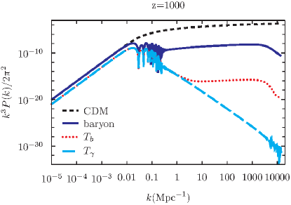
The evolution of small-scale perturbations, therefore, is coupled to large-scale perturbations on which they are sitting. Ignoring the terms in square brackets, and shifting the viewpoint to the CDM rest frame in which (as in O’Leary & McQuinn 2012; TH chose the baryon rest frame), Equation (10), in the -space, finally becomes
| (11) | |||||
where , and now denote fluctuations in the -space while , and are fluctuations of a given patch at in the space, given by Equation (7).
2.2 Evolution of perturbation inside patches: Numerical Scheme
Evolution of small-scale perturbations can be calculated by integrating the rate equation (Equation 11) from some initial redshift, preferentially not too long after the recombination epoch when the relative motion has not yet influenced the evolution. We take as the initial redshift. The initial condition should be generated for both the background quantities and the small-scale modes. For the background, as perturbations in Equation (11) are -space quantities whose distributions are all Gaussian, one needs to sample these values in the -space accordingly. For the small-scale modes, one just needs to track the evolution of the average value in the -space.
Let us first describe the statistics of background patches that we expect. TH calculated the evolution of small-scale () fluctuations under different background patches but only of , and defined “local power spectrum” averaged out over all possible opening angles between and . In our case, there are extra dimensions to consider which are , , , and , resulting in a much higher computational demand. Fortunately, some of these quantities are in perfect correlation with one another with linear proportionality. In addition, their initial values at completely compose the ensemble at any time through Equation (7). At the minimal level222For a more accurate treatment or for a specific patch of interest, one should also consider variations in other variables, such that . As the correlation between () and () becomes tighter in time, the initial variation gets gradually diluted, which roughly justifies our restricting the parameter space only to and ., it would suffice to just consider variation of in addition to such that the local power spectrum is an explicit function of the two background quantities, or .
For the initial condition for background patches, we generate 3D maps of , , , , , , and at on uniform grid cells inside a cubical volume of . We generate fluctuations of discrete modes that are randomized as
| (12) |
for given , where and are random numbers drawn from mutually independent Gaussian distributions with mean 0 and standard deviation 1, stands for any kind of -space fluctuations, and TF is the transfer function of , whose sign should be multiplied because some ’s oscillate around zero in . The configuration is roughly equivalent to applying a smoothing filter of length Mpc. In practice, we use CAMB (Lewis et al. 2000) for , and use the continuity equations () for , with the help of two CAMB transfer-function outputs at mutually nearby redshifts for time differentiation. is obtained from the relation . is fixed by following the scheme by Naoz & Barkana (2005): we require at the initial redshift in Equation (4), which results in
| (13) |
where all quantities are evaluated at , especially with the help of Equation (7) for and two adjacent CAMB transfer-function outputs for . Finally, all these -space fluctuations are Fourier-transformed to obtain -space fluctuations.
3D maps and 2D histograms of several initial quantities are presented in Figure 2. Fields of and on a part of a slice of the box at are shown in Figure 2(a). As expected, the velocity field converges on overdense regions and diverges on underdense regions. We find that in most patches dominates over , and thus the map of looks very similar to Figure 2(a). This occurs because baryons lag behind CDMs due to their coupling to CMB. (Figure 2b) is coupled to (Figure 2c) more strongly than to . and (similarly and ) are almost perfectly correlated (Figure 2d). and are very loosely correlated due to the tight coupling of baryons to photons at the redshift (Figure 2e), but the correlation becomes tighter in time. and are not correlated (Figure 2f). Because of this fact, the probability distribution function (PDF) is simply a multiplication of PDFs and , at the minimal level. Due to Gaussianity at , we have
| (14) |
where and are the standard deviations of and projected onto one Cartesian-coordinate axis, respectively. With our setup, we find that and km/s at (or the root-mean-square of is km/s). At the minimal level of only allowing the variance in and , the average power spectrum will then be given by the ensemble average
| (15) | |||||
where the PDFs and integral arguments are the ones at . Of course, a more accurate and straightforward way is to just ensemble-average over the patches from a large-box realization, because for example and are too poorly correlated at .
We numerically integrate Equation (11) to examine the evolution of small-scale (high-) fluctuations at any overdense (underdense) patch to the linear order, with the help of Equations (7) and (9) for the evolution of background quantities. In practice, we used the ODE45 modules of MATLAB®(2015b, The MathWorks, Inc., Natick, Massachusetts, United States) and of GNU Octave, which use the 4th-order Runge-Kutta method, with the relative tolerance and the absolute tolerance . During the evolution, the number of integration steps is the highest for , because its amplitude changes from the initial, very small values around to final, much larger values close to . Therefore, taking sub-steps for while coarser steps for other ’s is expected to boost the computational efficiency, even though we did not yet implement the method in our computation. The end result is then ensemble-averaged over varying and to obtain (Equation 15).
3 Result
3.1 Power spectrum of the matter density
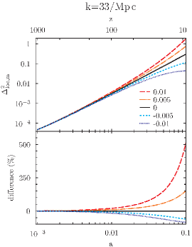
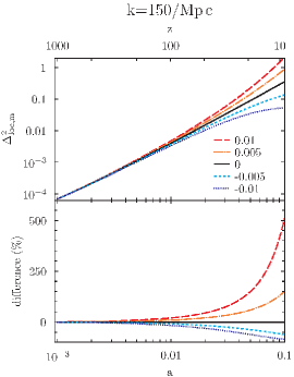
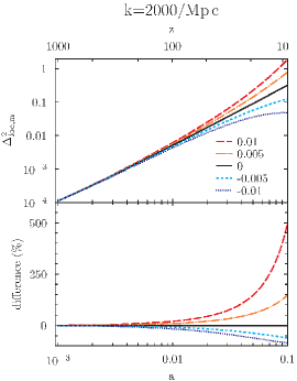
We first examine how the evolution of depends on the density environment, and compare the result to the prediction by TH. Figure 3 shows the evolution of of three arbitrarily chosen wave numbers (={33, 150, 2000} /Mpc) when in different density environments (={-0.01, -0.005, 0, 0.005, 0.01}). Note again that at , and thus these samples correspond to and . First, as expected, the growth of small-scale fluctuations are biased when and anti-biased when , with respect to the mean-density case (prediction by TH). Secondly, when ’s are equal in amplitude but opposite in sign, the deviations of from reveal the same trend but only until when and when . Afterwards, the bias and the anti-bias are not balanced by more than 1% and such off-balance keeps growing in time. The higher the is, the earlier this unbalance starts. Thirdly, the fractional deviation from the mean-density case is almost universal regardless of the value of , and thus the timing of the unbalance is approximately a function only of . Finally, in some high- patches, our linear analysis based on Equation (11) without quadratic and higher-order terms in starts to break down at , because these modes enter the nonlinear regime (; see Figure 3) at this epoch. A similar breakdown of the formalism will occur for perturbations inside very low- patches as well. Therefore, a higher-order scheme than our work is required when one is to predict the low-redshift evolution of ’s. On the other hand, if one were to generate initial conditions for numerical simulations in the linear regime, our formalism would provide the sufficient accuracy.
How large-scale overdensity impacts the evolution of small-scale inhomogeneities is reflected in the density continuity equation. In overdense background patches, grows in time and . Then, in Equation (11), and work as sources terms in addition to to the growth of . This will boost the growth rate of of both overdense (, ) and underdense (, ) modes. In contrast, in underdense background patches, these terms suppress the growth rate of of both overdense and underdense modes. The distribution of is Gaussian, and therefore for each “bias” case with there exists an “anti-bias” case with . Nevertheless, the unbalance described above is expected to boost the average power spectrum from that by TH.
The overall effect of including the Gaussian distribution of is thus to mitigate the negative impact by the relative velocity, predicted by TH, to some extent. In addition, the universality of the unbalance in boosts even in the range ( and ) where the power spectrum is almost unaffected by non-zero (Figure 4 shown in terms of the -space matter-density variance ). Note that the result for cannot be trusted, because our perturbation theory is based on the condition that large-scale modes () are well separated from small-scale modes in scale. Discrepancy of including non-zero ’s from the prediction by TH is negligible at , but later the discrepancy grows in time. Of course, individual patches may experience discrepancy in much earlier than this epoch (Figure 3).
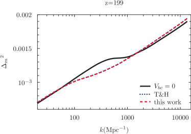
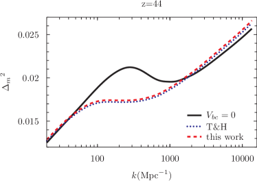
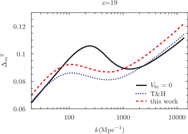
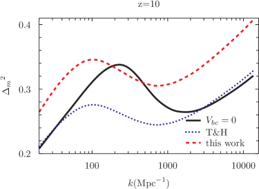
3.2 Halo abundance
Understanding the abundance and the spatial distribution of cosmological halos is crucial in modern astrophysics and cosmology. In this section, we examine the halo abundance both in the local and the global sense, just as we did for the matter power spectrum.
Let us first revisit the calculation by TH. They adopted the extended Press-Schechter formalism and calculated the local halo abundance, in terms of the conditional mass function, using the peak-background split scheme. A patch with (let us use this notation for the matter overdensity, to avoid confusion with the -space matter-density variance ) and will have the number of halos per unit Eulerian comoving volume per given by
| (16) | |||||
where is the critical overdensity of spherical collapse, and is the variance of density field smoothed with the window function corresponding to mass ,
| (17) |
One should note that should be that of high modes only, or more accurately a reduced value where is the variance of density field smoothed with the window function corresponding to the mass of the patch333It is not clear whether TH used this reduced variance. In addition, a factor of 2 should be multiplied to Equation (18) of TH. (e.g. Bond et al. 1991; Mo & White 1996; Ahn et al. 2015). One can instead put a lower bound () in the integral of Equation (17), which would be identical to the reduced variance if a sharp -space window function is used. The global mass function is simply an average of the local mass function, , over the ensemble of patches. When is averaged only over for a given , which is equivalent to visiting only those patches with the same and taking the average, it leads to the conditional mass function .
This calculation should be modified, because depends also on through the dependence of on :
| (18) |
which will enter Equation (16). Here we used the sharp -space filter, and thus . An overdense patch will then have a boost in from the value by TH because and thus , and vice versa (a decrease from the value by TH) for an underdense patch. Obviously, both and will also be affected.
It is important to compare our findings to the usual peak-background split scheme and the one by TH. In the “standard” scheme, if the density field is purely Gaussian, all the wave modes are assumed mutually independent in the linear regime. Therefore, the local, high- modes have a universal444Rigorously speaking, it is not perfectly universal because the lower bound changes slightly in as ). variance whether or not they are placed inside a patch with non-zero . The way how the halo formation is biased in an overdense region is simply through the shift in the density (). TH then realized the fact that the variance is not universal but should depend on . Because non-zero tends to suppress , the odds to cross decrease relative to the standard picture. We find that there is another dependency of the variance, which is . In other words, we find that there are two biasing effects in an overdense region compared to a mean-density region: getting closer to because of the shift in the density (, also in the standard scheme), and having a larger degree of fluctuation in due to the mode-mode coupling (e.g. source terms and in in Equation 11, which is a new finding). Therefore, by not fully implementing the effect of non-zero , TH in effect underestimates and overestimates the halo mass functions in overdense and underdense regions, respectively.
We note that this additional bias effect should be present even in the standard picture with , because this is due to the natural coupling between the large-scale and small-scale density perturbations. In this case, however, we are not sure about the quantitative validity of the extended Press-Schechter formalism on the conditional mass function (Equation 16), which is based on the linear theory guaranteeing Gaussianity at any filtering scales without the mode-mode couplings. Qualitatively, we believe that the boost of local and under should boost the conditional mass function to the level estimated by Equations (16) and (18) as described above anyways. We defer a further investigation of this issue, which can be clarified with numerical simulations of the halo formation under different ’s.
Discrepancy between the conditional mass functions by this work and by TH is significant if we focus on individual patches. Figure 5 illustrates how our prediction differs from that by TH. For example, at , under we predict [100 - 2000] % boost in compared to the values by TH (let us denote them by ). For , we predict 90 % or more decrease in compared to the values by TH. This is the obvious result of the mode-mode coupling of and described above. It is also noteworthy that the discrepancy is the largest for the rarest halos: first, at any redshift, the discrepancy increases as the halo mass increases and secondly, for any given halo mass, the discrepancy decreases in time.
The discrepancy among the conditional mass functions by this work, by TH and by the standard picture also influences . Let us just take the example of (Figure 6). Compared to the standard prediction (), conditional mass functions by TH stay lower regardless of . This is due to the suppression of structure formation by the relative velocity. In contrast, in this work is either higher or lower than the standard prediction () depending on the halo mass and . At , for and for for any halo mass. The tendency for to overshoot when is not generic, because the influence of the positive ’s on the structure formation appears only late in its evolution (see Figs. 3 and 4). At any rate, the contrast in among overdense and underdense regions is increased compared to TH and the standard picture, and the net effect e.g. at is to boost from . At much higher redshifts, our is almost indistinguishable from that by TH, which undershoots .
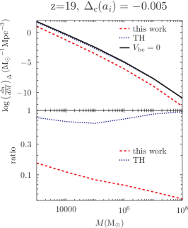
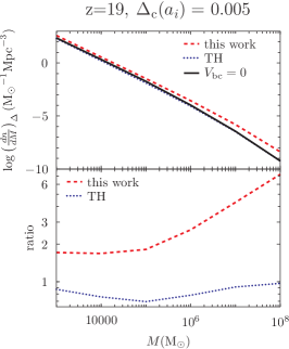
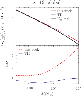
We note that and have the usual problem of not correctly predicting the actual mass function, if one sticks to the original extended Press-Schechter formalism. Minihalos at high redshifts are usually underestimated by the extended Press-Schechter formalism. The usual peak-background split method suffers from large discrepancies between its prediction and the N-body simulation results for rare halos in general. In this case, a hybrid method to connect the peak-background-split halo bias parameter to the better-fitting mean mass function types (e.g. Barkana & Loeb 2004; Ahn et al. 2015) is much more appropriate. We will apply this method in the future for a better estimation of the conditional mass function and the -space halo bias parameter (Section 3.3).
3.3 Halo bias and stochasticity
The conditional mass function we examined in Section 3.2 is an indicator of how halo formation is biased toward overdense regions. The halo bias can be viewed also in the the -space. This is a crucial parameter in cosmology when trying to probe the fluctuation of the matter density from surveys of galaxies through, for example, the power spectrum analysis.
The halo bias parameter in -space is defined as
| (19) |
where is the power spectrum of halo over-abundance
| (20) |
can then be Fourier-transformed in order to calculate . We expect to be larger than that predicted by TH, because the “contrast” in between overdense and underdense regions has increased from that by TH (Section 3.2; Figure 5). This is clearly seen in Figure 7, where we show ’s computed in this work and by TH. At and for , we find that is about times as large as the one by TH. This is again caused by the mode-mode coupling.
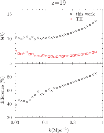
As was pointed out by TH, oscillates in due to the baryonic acoustic oscillations (BAO)555Our box size is barely larger than the BAO scale, and is thus too small to accurately estimate at low ’s. We will increase the size of the box in future work for a better estimation., which is tied to the modulation of the streaming velocity, the density fluctuation, and the baryon fraction in the existence of the compensated mode (Barkana & Loeb, 2011). This makes it difficult to deduce from , not to mention from the galaxy surveys where galaxy formation mechanism, strongly influenced by baryonic physics, is another nuisance parameter (but see Slepian & Eisenstein 2015 for how to separate out the streaming velocity effect). For the halo mass range treated in this paper, should modulate the distribution of the first stars which grow predominantly inside minihalos. As was also noted by TH, the difference in should also influence the formation of much larger-mass halos, which are used for galaxy surveys. It is also possible that the nonlinear effect described by O’Leary & McQuinn (2012), or the heating of the intergalactic medium (IGM) due to the velocity difference between CDM and baryons, is modulated in space depending on the overdensity. Then the power spectrum in the 21-cm background, which may be dominated by the velocity fields if the heating is efficient (McQuinn & O’Leary 2012), is likely to be boosted. Because such a power spectrum shows a very clear BAO feature and the 21-cm observation usually suffers from the low sensitivity, the signal boosted even more from the prediction by McQuinn & O’Leary (2012) will be a very promising target for the high-redshift 21-cm cosmology.
Let us briefly discuss the halo stochasticity. The halo stochasticity is defined as
| (21) |
where is the cross power spectrum between the halo density and the matter density. Both in TH and in this work, stochasticity is caused by the fluctuation in because patches with the same can have different ’s which affect . One should note that the fluctuation should be caused also by the sampling variance. The conditional mass functions usually show super-Poissonian distributions in even in the standard picture with (e.g. Saslaw & Hamilton 1984; Sheth 1995; Neyrinck et al. 2014; Ahn et al. 2015), and obviously this should cause the stochasticity in addition to that by the varying . Because we use the “mean” conditional mass function just as TH did, in both works does not reflect the sampling variance. Including this effect requires the calculation of the sub-cell correlation function (Ahn et al. 2015), which we delay to future work.
4 Discussion
We investigated the impact of the relative velocity (streaming velocity) between CDM and baryons on the small-scale structure formation. TH first studied this effect by adopting a trivial solution to the large-scale velocity and density fields. Because velocity fields are correlated with density fields, however, such a trivial solution cannot accurately describe the physics in regions with non-zero overdensity. We thus improved on the work by TH by implementing a non-trivial solution to the large-scale velocity and density fields, and we find that this causes a new type of coupling between large-scale and small-scale modes. This results in boosting the small-scale structure formation in overdense regions and suppressing that in underdense regions, aside from the suppression originating from the streaming velocity. The net effect on the structure formation is to boost the overall fluctuation, in terms of , and thus the “negative” effect by TH is mitigated to some extent. Depending on the wave mode () and the observing redshift, can even be larger than that in the standard picture with . The conditional halo mass function and the halo bias are also affected in similar ways.
The results of this work show that the formation and evolution of small-scale structures depend strongly on not only the streaming velocity but also the density environment. The most important aspect of our work is that in contrast to TH, who predict that regardless of the underlying density the local matter power spectrum of small-scale structures will be identical as long as is the same, the underlying large-scale ( a few Mpc) overdensity is another key parameter in addition to . This then requires re-examining previous work based on the formalism by TH. We already showed that , , , , and are affected. If one were to simulate the nonlinear evolution of density perturbations and the structure formation in Mpc patches, he should generate initial conditions based on this work. As is seen in Figure 3, we cannot neglect the impact of overdensity even when the simulation starts at e.g. , because at the discrepancy between our prediction and that by TH is already a few percent at that redshift.
Both the previous semi-analytical work (Tseliakhovich et al. 2011; Fialkov et al. 2012; McQuinn & O’Leary 2012; Bovy & Dvorkin 2013; Naoz & Narayan 2014; Asaba et al. 2016) and the semi-numerical work (e.g. Fialkov et al. 2013; Visbal et al. 2012) should be re-examined. Attempts to numerically simulate the nonlinear evolution of small-scale structures have been mostly limited to the physics inside mean-density regions (McQuinn & O’Leary 2012; Maio et al. 2011; Stacy et al. 2011; Greif et al. 2011) or special, isolated regions (Tanaka & Li 2014). These numerical simulations thus need to be extended to incorporate which varies in space. In doing so, a reasonable method would be to use adaptive mesh refinement (AMR) codes with nested grids, so that one or a few interesting regions (Mpc patches with , for example) are treated with fine meshes and other regions with coarse meshes for computational efficiency.
We also showed that cosmology through galaxy surveys should carefully consider the impact of the mode-mode couping, because the halo bias (and galaxy bias as well) would be boosted from not only the standard prediction with but also the prediction by TH. Cosmology with the intensity mapping may also be affected. The post-reionization intensity mapping targets the large-angle, diffuse 21-cm background from neutral hydrogen atoms inside galaxies (Chang et al. 2008; Abdalla et al. 2010; Bandura et al. 2014; Xu et al. 2015). Because any galaxies, small or large, contribute to this cumulative 21-cm background, such observations will be affected by the streaming velocity through . The pre-reionization intensity mapping targets the large-angle, diffuse 21-cm background from the intergalactic neutral hydrogen atoms (Scott & Rees 1990; Bharadwaj & Ali 2004; Loeb & Zaldarriaga 2004; Barkana & Loeb 2005; McQuinn et al. 2006; ; Mao et al. 2012; Shapiro et al. 2013). Even though this is free from the galaxy bias, the streaming velocity may act as a heating mechanism and boost the power spectrum of the velocity field (McQuinn & O’Leary 2012), and therefore the new findings of our work should be incorporated.
Application to the study of the cosmic reionization process is of a prime interest in terms of the high-redshift astrophysics. The complex nature of the process usually requires numerical simulations, and they are performed through either efficient semi-numerical methods (Furlanetto et al. 2004; McQuinn et al. 2007; Mesinger et al. 2011; Alvarez & Abel 2012) or fully numerical methods (e.g. Gnedin & Abel 2001; Razoumov et al. 2002; Maselli et al. 2003; Mellema et al. 2006; Baek et al. 2009; Wise & Abel 2011). The early phase of cosmic reionization must have been driven by the first stars, possibly forming first in minihalos, as these are the first luminous objects in the universe. A very important factor that modulates the formation of the first stars inside minihalos is the Lyman-Werner intensity, which have been properly treated in simulations in a box large enough for statistical reliability but implementing subgrid physics for the first star formation inside minihalos (Ahn et al. 2012; Fialkov et al. 2013). To predict reionization scenarios to our best knowledge, especially on its early phase, this work should be properly incorporated because the star formation inside minihalos is strongly modulated by the streaming velocity as well.
The results of this paper have rooms for further improvements. This paper is based on the presumption that the fluctuations at a few Mpc scale remain linear even at later epochs. However, high density regions will reach the nonlinear regime earlier than the rest, and then our formalism will break down in such regions. The halo bias is more strongly pronounced in the nonlinear patches (e.g. Ahn et al. 2015) than in the linear theory, and thus one should use the actual values of the overdensity in such circumstances. One could achieve this goal by adopting the quasi nonlinear calculation (e.g. 2LPT by Crocce et al. 2006), adopting the top-hat collapse model as in Mo & White (1996) and Ahn et al. (2015), or for the best accuracy running N-body+hydro simulations which resolve the density fluctuation at Mpc scale. Then, in each patch of a few comoving Mpc, Equation (11) can be integrated with the newly computed values of ’s. Wave modes in the range Mpc are not accurately treated, because we based our formalism on the separability of the large-scale modes (Mpc) and the small-scale modes (Mpc). The code we used will be released for the public use, but it requires technical improvements such as allowing parallel computation and porting to more generic computation languages. We will maintain and control its development through the website http://www.chosun.ac.kr/kjahn.
Appendix A Normal Modes for the large-scale fluctuations
When the fluctuation of radiation components are neglected, the growth of large-scale density and velocity fluctuations are well approximated by Equations (5) and (6). Their evolution can then be described by the 4 normal modes described in Section 2.1. The growing and decaying modes are the two solutions to the second-order equation
| (A1) |
where , and can be written also as
| (A2) |
Similarly, the compensated and streaming modes are the two solutions to
| (A3) |
where , and can be written also as
| (A4) |
We now take a convention of writing each mode as the product of its initial value at and its growth factor: , , , and , denoting the growing, decaying, compensated, and streaming modes, respectively. These modes comprise and , as and , with the normalization at .
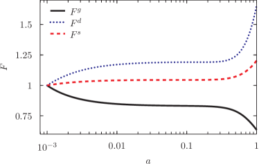
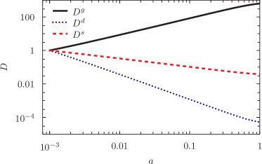
The first task in finding these modes is to calculate the growth factors. Because the Hubble constant ( and have non-negligible radiation components during the period of interest, , growth factors should be calculated numerically. We factor out deviations from the analytical form valid during the matter-dominated () era, as , , and , and then solve for the order-of-unity values of , , and . They are determined by
| (A5) |
| (A6) |
and
| (A7) |
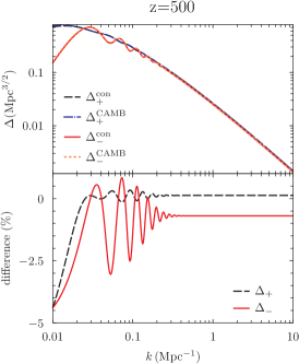
In practice, the numerical integration of Equations (A5)-(A7) is started at (backward for and forward for ), with the condition that at because it is a matter-dominated epoch, and at because of our normalization convention. One can instead start the integration from the radiation dominated epoch (just numerically assuming that Equations (A5)-(A7) are all valid at and using the asymptotes for and at that time), but we find that Equations (A6) and (A7) become stiff if integrated forward in increasing at high . We show the growth factors found this way in Figure 8.
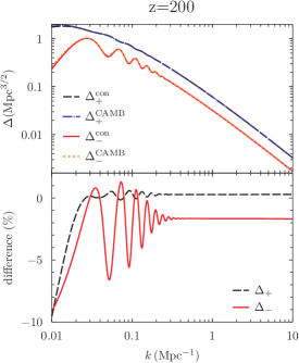
Now we can find the initial values of these modes by using the growth factors found above on the transfer function outputs from CAMB. We algebraically relate two redshift outputs, at and in practice, to find these modes:
| (A8) |
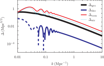
where are those from CAMB. The modes found this way are shown in Figure 9.
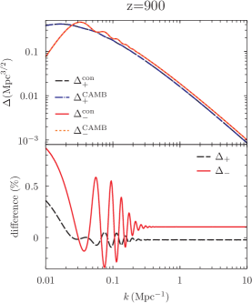
A few things are notable. An unperturbed Hubble flow requires , while we find that at and is not constant over . Even though one can choose different redshifts to extract these modes and they should not change in principle, the resulting modes at vary depeding on the choice of the redshifts. We believe that this is partly due to our neglect of the fluctuations of radiation components, because they can affect the evolution of density fluctuations. We find that our current choice of and is optimal for : using these modes and evolving them with the growth factors, we find a good match between , “constructed” by using these modes and those calculated by CAMB, at any redshifts with at most a several percent error. We show their comparison in Figure 10.
Schmidt (2016) follows a similar approach for the mode extraction but uses CAMB transfer function outputs at . Their focus is on the low-redshift galaxy surveys, and thus the accuracy is required mostly at and near the present. In our case, accuracy in and is required mostly at a high redshift range, , because the small-scale modes are continuously affected by large-scale modes from the epoch of recombination and the linear perturbation analysis on small-scales modes breaks down later when they become nonlinear.
Appendix B Fitting formula for the large-scale temperature fluctuation
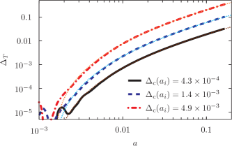
For the evolution of , we integrate Equation (8) on each spatial patch. Early on, its value is strongly affected by the initial fluctuation of the CMB temperature. Later, it decouples from the CMB fluctuation and is determined mostly by . Therefore, one expects a strong correlation between and long after recombination. For example, at and , they follow the linear relation: at , and at . Regardless of the variance in , therefore, one can find a fitting formula for after its decoupling from the CMB temperature.
The fitting formula is given by Equation (9). We note that Equation (9) is valid only when the patch size is 4 comoving Mpc. For patches in different size, we believe that a generic form of a two-parameter fit,
| (B1) |
will serve as a good fit regardless of the patch size. The linear relation between and at and can be found by comparing the two quantities. In case of the 4 comoving Mpc patch, we find that and (Equation 9) provides an excellent fit to when , with the linear relations at and at This is demonstrated in Figure 11, where the evolution of different ’s are shown depending on the initial , together with the corresponding fits.
References
- Abdalla et al. (2010) Abdalla, F. B., Blake, C., & Rawlings, S. 2010, MNRAS, 401, 743
- Ahn et al. (2012) Ahn, K., Iliev, I. T., Shapiro, P. R., et al. 2012, ApJ, 756, L16
- Ahn et al. (2015) Ahn, K., Iliev, I. T., Shapiro, P. R., & Srisawat, C. 2015, MNRAS, 450, 1486
- Alvarez & Abel (2012) Alvarez, M. A., & Abel, T. 2012, ApJ, 747, 126
- Asaba et al. (2016) Asaba, S., Ichiki, K., & Tashiro, H. 2016, Phys. Rev. D, 93, 023518
- Baek et al. (2009) Baek, S., Di Matteo, P., Semelin, B., Combes, F., & Revaz, Y. 2009, A&A, 495, 389
- Bandura et al. (2014) Bandura, K., Addison, G. E., Amiri, M., et al. 2014, in Proc. SPIE, Vol. 9145, Ground-based and Airborne Telescopes V, 914522
- Barkana & Loeb (2004) Barkana, R., & Loeb, A. 2004, ApJ, 609, 474
- Barkana & Loeb (2005) —. 2005, ApJ, 624, L65
- Barkana & Loeb (2011) —. 2011, MNRAS, 415, 3113
- Bernardeau et al. (2002) Bernardeau, F., Colombi, S., Gaztañaga, E., & Scoccimarro, R. 2002, Phys. Rep., 367, 1
- Bharadwaj & Ali (2004) Bharadwaj, S., & Ali, S. S. 2004, MNRAS, 352, 142
- Blazek et al. (2015) Blazek, J., McEwen, J. E., & Hirata, C. M. 2015, ArXiv e-prints, arXiv:1510.03554
- Bond et al. (1991) Bond, J. R., Cole, S., Efstathiou, G., & Kaiser, N. 1991, ApJ, 379, 440
- Bovy & Dvorkin (2013) Bovy, J., & Dvorkin, C. 2013, ApJ, 768, 70
- Chang et al. (2008) Chang, T.-C., Pen, U.-L., Peterson, J. B., & McDonald, P. 2008, Physical Review Letters, 100, 091303
- Crocce et al. (2006) Crocce, M., Pueblas, S., & Scoccimarro, R. 2006, MNRAS, 373, 369
- Dalal et al. (2010) Dalal, N., Pen, U.-L., & Seljak, U. 2010, J. Cosmology Astropart. Phys, 11, 007
- Fialkov et al. (2012) Fialkov, A., Barkana, R., Tseliakhovich, D., & Hirata, C. M. 2012, MNRAS, 424, 1335
- Fialkov et al. (2013) Fialkov, A., Barkana, R., Visbal, E., Tseliakhovich, D., & Hirata, C. M. 2013, MNRAS, 432, 2909
- Furlanetto et al. (2004) Furlanetto, S. R., Zaldarriaga, M., & Hernquist, L. 2004, ApJ, 613, 1
- Gnedin & Abel (2001) Gnedin, N. Y., & Abel, T. 2001, New Astronomy, 6, 437
- Greif et al. (2011) Greif, T. H., White, S. D. M., Klessen, R. S., & Springel, V. 2011, ApJ, 736, 147
- Komatsu et al. (2011) Komatsu, E., Smith, K. M., Dunkley, J., et al. 2011, ApJS, 192, 18
- Lewandowski et al. (2015) Lewandowski, M., Perko, A., & Senatore, L. 2015, J. Cosmology Astropart. Phys, 5, 019
- Lewis et al. (2000) Lewis, A., Challinor, A., & Lasenby, A. 2000, Astrophys. J., 538, 473
- Loeb & Zaldarriaga (2004) Loeb, A., & Zaldarriaga, M. 2004, Physical Review Letters, 92, 211301
- Maio et al. (2011) Maio, U., Koopmans, L. V. E., & Ciardi, B. 2011, MNRAS, 412, L40
- Mao et al. (2012) Mao, Y., Shapiro, P. R., Mellema, G., et al. 2012, MNRAS, 422, 926
- Maselli et al. (2003) Maselli, A., Ferrara, A., & Ciardi, B. 2003, MNRAS, 345, 379
- McQuinn et al. (2007) McQuinn, M., Lidz, A., Zahn, O., et al. 2007, MNRAS, 377, 1043
- McQuinn & O’Leary (2012) McQuinn, M., & O’Leary, R. M. 2012, ApJ, 760, 3
- McQuinn et al. (2006) McQuinn, M., Zahn, O., Zaldarriaga, M., Hernquist, L., & Furlanetto, S. R. 2006, ApJ, 653, 815
- Mellema et al. (2006) Mellema, G., Iliev, I. T., Alvarez, M. A., & Shapiro, P. R. 2006, New A, 11, 374
- Mesinger et al. (2011) Mesinger, A., Furlanetto, S., & Cen, R. 2011, MNRAS, 411, 955
- Mo & White (1996) Mo, H. J., & White, S. D. M. 1996, MNRAS, 282, 347
- Naoz & Barkana (2005) Naoz, S., & Barkana, R. 2005, MNRAS, 362, 1047
- Naoz & Narayan (2013) Naoz, S., & Narayan, R. 2013, Physical Review Letters, 111, 051303
- Naoz & Narayan (2014) —. 2014, ApJ, 791, L8
- Naoz et al. (2012) Naoz, S., Yoshida, N., & Gnedin, N. Y. 2012, ApJ, 747, 128
- Neyrinck et al. (2014) Neyrinck, M. C., Aragón-Calvo, M. A., Jeong, D., & Wang, X. 2014, MNRAS, 441, 646
- O’Leary & McQuinn (2012) O’Leary, R. M., & McQuinn, M. 2012, ApJ, 760, 4
- Planck Collaboration et al. (2015) Planck Collaboration, Ade, P. A. R., Aghanim, N., et al. 2015, ArXiv e-prints, arXiv:1502.01589
- Popa et al. (2015) Popa, C., Naoz, S., Marinacci, F., & Vogelsberger, M. 2015, ArXiv e-prints, arXiv:1512.06862
- Razoumov et al. (2002) Razoumov, A. O., Norman, M. L., Abel, T., & Scott, D. 2002, ApJ, 572, 695
- Reichardt et al. (2012) Reichardt, C. L., Shaw, L., Zahn, O., et al. 2012, ApJ, 755, 70
- Richardson et al. (2013) Richardson, M. L. A., Scannapieco, E., & Thacker, R. J. 2013, ApJ, 771, 81
- Saslaw & Hamilton (1984) Saslaw, W. C., & Hamilton, A. J. S. 1984, ApJ, 276, 13
- Schmidt (2016) Schmidt, F. 2016, ArXiv e-prints, arXiv:1602.09059
- Scott & Rees (1990) Scott, D., & Rees, M. J. 1990, MNRAS, 247, 510
- Shapiro et al. (2013) Shapiro, P. R., Mao, Y., Iliev, I. T., et al. 2013, Phys. Rev. Lett., 110, 151301
- Sheth (1995) Sheth, R. K. 1995, MNRAS, 274, 213
- Shoji & Komatsu (2009) Shoji, M., & Komatsu, E. 2009, ApJ, 700, 705
- Slepian & Eisenstein (2015) Slepian, Z., & Eisenstein, D. J. 2015, MNRAS, 448, 9
- Somogyi & Smith (2010) Somogyi, G., & Smith, R. E. 2010, Phys. Rev. D, 81, 023524
- Stacy et al. (2011) Stacy, A., Bromm, V., & Loeb, A. 2011, ApJ, 730, L1+
- Tanaka & Li (2014) Tanaka, T. L., & Li, M. 2014, MNRAS, 439, 1092
- Tanaka et al. (2013) Tanaka, T. L., Li, M., & Haiman, Z. 2013, MNRAS, 435, 3559
- Tseliakhovich et al. (2011) Tseliakhovich, D., Barkana, R., & Hirata, C. M. 2011, MNRAS, 418, 906
- Tseliakhovich & Hirata (2010) Tseliakhovich, D., & Hirata, C. 2010, Phys. Rev. D, 82, 083520
- Visbal et al. (2012) Visbal, E., Barkana, R., Fialkov, A., Tseliakhovich, D., & Hirata, C. M. 2012, Nature, 487, 70
- Wise & Abel (2011) Wise, J. H., & Abel, T. 2011, MNRAS, 414, 3458
- Xu et al. (2015) Xu, Y., Wang, X., & Chen, X. 2015, ApJ, 798, 40
- Yoo et al. (2011) Yoo, J., Dalal, N., & Seljak, U. 2011, J. Cosmology Astropart. Phys, 7, 018