Complementarity of genuine multipartite (Bell) non-locality

Sasha Sami Center for Security, Theory and Algorithmic Research, International Institute of Information Technology, Gachibowli, Hyderabad, India.    Anubhav Chaturvedi anubhav.chaturvedi@research.iiit.ac.in Center for Security, Theory and Algorithmic Research, International Institute of Information Technology, Gachibowli, Hyderabad, India. Institute of Theoretical Physics and Astrophysics, National Quantum Information Centre, Faculty of Mathematics, Physics and Informatics, University of Gdańsk, Wita Stwosza 57, 80-308 Gdańsk, Poland    Indranil Chakrabarty Center for Security, Theory and Algorithmic Research, International Institute of Information Technology, Gachibowli, Hyderabad, India.
Abstract

We introduce a new feature of no-signaling (Bell) non-local theories, namely, when a system of multiple parties manifests genuine non-local correlation, then there cannot be arbitrarily high non-local correlation among any subset of the parties. We call this feature, complementarity of genuine multipartite non-locality. We use Svetlichny’s criterion for genuine multipartite non-locality and non-local games to derive the complementarity relations under no-signaling constraints. We find that the complementarity relations are tightened for the much stricter quantum constraints. We compare this notion with the well-known notion of monogamy of non-locality. As a consequence, we obtain tighter non-trivial monogamy relations that take into account genuine multipartite non-locality. Furthermore, we provide numerical evidence showcasing this feature using a bipartite measure and several other well-known tripartite measures of non-locality.

I Introduction

In 1964 John Stewart Bell established the fact that no physical theory of local hidden variables can reproduce all of the predictions of quantum mechanics Bell (1964, 1966); Brunner et al. (2014). An inequality was designed to illustrate the same. This inequality, now commonly referred to as the Bell’s inequality, was based on the assumptions of local realism Clauser et al. (1969); Freedman and Clauser (1972); i.e. the inequality is satisfied by all possible statistics admitted by local-real (local hidden variable) models. The phenomenon of the violation of this inequality is commonly referred to as (Bell) non-locality. The term ‘non-locality’ is a misnomer, in this work we use the term to imply the departure of the predictions of the theory under consideration from the predictions of any local-real (local hidden variable) model. In quantum theory, certain states (for instance, the singlet) violate the Bell’s inequality, deeming the theory to be non-local. However, the notion of non-locality is not restricted to the quantum theory; i.e., in general the statistics predicted by any theory which violates the Bell’s inequality cannot be explained by a local hidden variable model and the theory can be regarded as being non-local. The amount of violation of the Bell-inequality serves as a metric for non-locality; i.e., it quantifies just how far the predictions of a particular operational theory are from that of the local hidden variable models. For instance, it is known that the no-signaling condition allows more non-locality than what is admitted by the quantum theory Barrett and Pironio (2005); Chakrabarty et al. (2014). The amount of non-locality is directly associated with the advantage in many information processing protocols and tasks, when using non-local resources as compared to when using classical (local-real) resources Horodecki et al. (1996); Adhikari et al. (2008); Chakrabarty et al. (2011); Chaturvedi and Banik (2015).
The notion of non-locality as presented in the Bell’s theorem was restricted to bipartite systems. The extension of the notion of non-locality to multipartite systems presents itself with delicate intricacies Brunner et al. (2014). Let us consider a tripartite system. A well known Bell-type inequality, now commonly known as the Mermin’s inequality Mermin (1980, 1990), is based on the assumption that all three systems are locally correlated; i.e., the inequality is satisfied by all possible statistics of the tripartite system that can be explained by local-real models. A violation of this inequality simply implies non-locality. A bipartite non-local system locally correlated with the third system violates this inequality. The observation of this fact preceded the search for Bell-type inequalities that would distill genuine tripartite non-locality; i.e., non-locality vested in all three systems combined. Svetlichny gave a systematic way of characterizing genuine tripartite non-locality along-with an inequality, now commonly referred to as the Svetlichny’s inequality Svetlichny (1987). This stronger inequality is based on the assumption of bi-locality which allows for non-locality in any bipartite subsystem locally correlated with the third system Svetlichny (1987). The violation of the Svetlichny’s inequality is a sufficient condition for witnessing genuine tripartite non-locality Bancal et al. (2011). The inequality itself is readily generalized to the multipartite scenario, wherein the Svetlichny’s set of inequalities form the sufficient conditions for witnessing genuine multipartite non-locality.
The notion of complementarity of physical phenomenon forms an integral part of the structure of quantum mechanics. Historically, soon after the conception of the uncertainty principle Heisenberg (1927), Neils Bohr brought up the notion of complementarity; i.e., physical systems described by the quantum theory have complementary properties which cannot all be observed or measured simultaneously, examples include, position and momentum, energy and duration, spin on different axes, and more Sazim et al. (2015). Recently, an interesting instance was brought up in the form of complementarity between tripartite quantum correlation and bipartite Bell-inequality violation Pandya et al. (2016).
In this work, we bring forth yet another instance of complementarity, but this time around without invoking the particulars of the quantum theory. We show that in any no-signaling non-local theory, witnessing genuine n𝑛n-party non-locality in a n𝑛n-party system, restricts the amount of genuine k𝑘k-party non-locality attainable by any of its k𝑘k-party subsystems. We use the Svetlichny’s criterion for genuine multipartite non-locality and the framework of non-local games to analytically proof our main result. We further find that the relations we derive, not only hold, but are tightened under the more restrictive quantum constraints. We also investigate the relationship between the prevalent notion of monogamy of non-locality and the notion of complementarity of genuine multipartite non-locality as presented in this work. As a consequence of this investigation, we find that in any no-signaling non-local theory the monogamy relations are tightened with increase in genuine multipartite non-locality. Furthermore, we provide numerical evidence in support of our main result, using other non-local games and inequalities in the simpler, tripartite vs. bipartite scenario.

II Preliminary concepts

In this section, we briefly discuss the notion of non-local games, their relation to Bell-type inequalities, followed by Svetlichny’s criterion of genuine multipartite non-locality. A reader familiar with these notions may consider continuing directly from the next section.

II.1 Non-local games

Non-local games are convenient constructs developed primarily for showcasing the power of non-locality as a resource Ambainis et al. (2013); Brunner et al. (2014). The non-local games were designed such that their associated winning probability severed as a metric to quantify the distance between the predictions of local-real models and the quantum theory. Now they are used to compare the predictions of other models and theories as well, for instance, the bi-local model, almost quantum models and the no-signaling framework. A non-local game is a cooperative task involving two or more spatially separated parties. These games are generally played against a referee. The parties are not allowed to communicate with each other during the task. However, they are allowed to share resources (typically, any amount of classical randomness and correlations allowed by the model under consideration) before the task begins.
In this work we consider non-local games involving n𝑛n parties A1,A2,Ansubscript𝐴1subscript𝐴2subscript𝐴𝑛A_{1},A_{2},\ldots A_{n}. For each round the referee assigns the i𝑖ith party an input bit xisubscript𝑥𝑖x_{i} and obtains an output bit uisubscript𝑢𝑖u_{i} from the i𝑖ith party. The players win the round if their outputs satisfy a particular condition, which may depend on the assignment of the inputs in that round. The measure of success in this task is simply the probability with which the players are able to satisfy the condition. For the rest of this paper, the winning condition is represented by a Boolean equation, say E𝐸E, defined over the input and output bits of the parties involved in the non-local game. Suppose that, the parties share a correlation represented by a conditional probability distribution p(u1,u2,un|x1,x2,xn)𝑝subscript𝑢1subscript𝑢2conditionalsubscript𝑢𝑛subscript𝑥1subscript𝑥2subscript𝑥𝑛p(u_{1},u_{2},\ldots u_{n}|x_{1},x_{2},\ldots x_{n}). Then the success probability of the non-local game is simply the probability with which the parties win or satisfy the equation E𝐸E, which is given by,

p(E)=12nEp(u1,u2,un|x1,x2,xn),𝑝𝐸1superscript2𝑛subscript𝐸𝑝subscript𝑢1subscript𝑢2conditionalsubscript𝑢𝑛subscript𝑥1subscript𝑥2subscript𝑥𝑛p(E)=\frac{1}{2^{n}}\sum_{E}p(u_{1},u_{2},\ldots u_{n}|x_{1},x_{2},\ldots x_{n}), (1)

where Esubscript𝐸\sum_{E} represents a sum over all inputs and outputs which satisfy E𝐸E.
Each Bell-type inequality comprises of a Bell-type expression and limit on this expression. This expression is usually a linear combination of expectations of products of outputs (in {+1,1}11\{+1,-1\}) of all the parties for particular input (measurement) settings. Each such Bell-type expression is inter-convertible with a non-local game, upon relabeling of outputs. To illustrate this, we shall now consider the case of two parties. Here we have the well known CHSH expression,

CHSH=x1=0,x2=0+x1=1,x2=0+x1=0,x2=1x1=1,x2=1.subscript𝐶𝐻𝑆𝐻delimited-⟨⟩formulae-sequencesubscript𝑥10subscript𝑥20delimited-⟨⟩formulae-sequencesubscript𝑥11subscript𝑥20delimited-⟨⟩formulae-sequencesubscript𝑥10subscript𝑥21delimited-⟨⟩formulae-sequencesubscript𝑥11subscript𝑥21\mathcal{I}_{CHSH}=\langle x_{1}=0,x_{2}=0\rangle+\langle x_{1}=1,x_{2}=0\rangle\\ +\langle x_{1}=0,x_{2}=1\rangle-\langle x_{1}=1,x_{2}=1\rangle. (2)

where x1=i,x2=jdelimited-⟨⟩formulae-sequencesubscript𝑥1𝑖subscript𝑥2𝑗\langle x_{1}=i,x_{2}=j\rangle is simply average over outcomes u1~,u2~{1,+1}~subscript𝑢1~subscript𝑢211\tilde{u_{1}},\tilde{u_{2}}\in\{-1,+1\} of parties A1,A2subscript𝐴1subscript𝐴2A_{1},A_{2} when x1=i,x2=jformulae-sequencesubscript𝑥1𝑖subscript𝑥2𝑗x_{1}=i,x_{2}=j, i.e.,

x1=i,x2=j=k,l{1,+1}(k.l)p(u~1=k,u~2=l|x1=i,x2=j).\langle x_{1}=i,x_{2}=j\rangle=\\ \sum_{k,l\in\{-1,+1\}}(k.l)p(\tilde{u}_{1}=k,\tilde{u}_{2}=l|x_{1}=i,x_{2}=j). (3)

While the Bell expressions use a ‘physicist’ notation; i.e, the outcomes take values in {1,+1}11\{-1,+1\}, non-local games utilize a ‘computer scientist’ notation; i.e., the outcomes take values in {0,1}01\{0,1\} Pironio et al. (2011). We can rewrite CHSHsubscript𝐶𝐻𝑆𝐻\mathcal{I}_{CHSH} as,

k,l,i,j{0,1}(1)klijp(u1=k,u2=l|x1=i,x2=j).\sum_{k,l,i,j\in\{0,1\}}(-1)^{k\oplus l\oplus ij}p(u_{1}=k,u_{2}=l|x_{1}=i,x_{2}=j). (4)

Now let us consider a non-local game described by the equation S2u1u2=x1x2subscript𝑆2direct-sumsubscript𝑢1subscript𝑢2subscript𝑥1subscript𝑥2S_{2}\equiv u_{1}\oplus u_{2}=x_{1}x_{2}. It straightforward to see that the winning probability of this non-local game is linearly related to the value of the CHSH expression; i.e,

p(S2)=S2p(u1,u2|x1,x2)=12(1+CHSH4),𝑝subscript𝑆2subscriptsubscript𝑆2𝑝subscript𝑢1conditionalsubscript𝑢2subscript𝑥1subscript𝑥2121subscript𝐶𝐻𝑆𝐻4p(S_{2})=\sum_{S_{2}}p(u_{1},u_{2}|x_{1},x_{2})=\frac{1}{2}\big{(}1+\frac{\mathcal{I}_{CHSH}}{4}\big{)}\;, (5)

which allows one to write the CHSH inequality in terms of the success probability of the non-local game represented by S2subscript𝑆2S_{2}; i.e.,

maxLV{|CHSH|}=2maxLV{p(S2)}=34,subscript𝐿𝑉subscript𝐶𝐻𝑆𝐻2subscript𝐿𝑉𝑝subscript𝑆234\max_{LV}\{|\mathcal{I}_{CHSH}|\}=2\equiv\\ \max_{LV}\{p(S_{2})\}=\frac{3}{4}, (6)

where maxLVsubscript𝐿𝑉\max_{LV} implies maximization over all possible statistics admitted by local hidden variable (local real) models.

II.2 Svetlichny’s criterion

Svetlichny’s criterion for genuine mulitpartite non-locality is applicable to a system of arbitrary number of spatially separated parties. But for the sake of a brief overview, we restrict to the case of three spatially separated parties A1,A2,A3subscript𝐴1subscript𝐴2subscript𝐴3A_{1},A_{2},A_{3}. Each party is assigned an input bit xisubscript𝑥𝑖x_{i} and obtains and output bit uisubscript𝑢𝑖u_{i} with i{1,2,3}𝑖123i\in\{1,2,3\}. The correlation shared by the three parties is represented by the joint probability distribution p(u1,u2,u3|x1,x2,x3)𝑝subscript𝑢1subscript𝑢2conditionalsubscript𝑢3subscript𝑥1subscript𝑥2subscript𝑥3p(u_{1},u_{2},u_{3}|x_{1},x_{2},x_{3}). This correlation would adhere to a local-real model if it can be decomposed as,

p(u1,u2,u3|x1,x2,x3)𝑝subscript𝑢1subscript𝑢2conditionalsubscript𝑢3subscript𝑥1subscript𝑥2subscript𝑥3\displaystyle p(u_{1},u_{2},u_{3}|x_{1},x_{2},x_{3})
=λq(λ)pλ(u1|x1)pλ(u2|x2)pλ(u3|x3),absentsubscript𝜆𝑞𝜆subscript𝑝𝜆conditionalsubscript𝑢1subscript𝑥1subscript𝑝𝜆conditionalsubscript𝑢2subscript𝑥2subscript𝑝𝜆conditionalsubscript𝑢3subscript𝑥3\displaystyle=\sum_{\lambda}q(\lambda)p_{\lambda}(u_{1}|x_{1})p_{\lambda}(u_{2}|x_{2})p_{\lambda}(u_{3}|x_{3}), (7)

where λ𝜆\lambda is the hidden variable and q(λ)𝑞𝜆q(\lambda) is the probability distribution governing λ𝜆\lambda, such that λq(λ)=1subscript𝜆𝑞𝜆1\sum_{\lambda}q(\lambda)=1. The correlations which cannot be written in this way are termed as being non-local. But in the multipartite scenario, there are many distinct forms of non-locality, some more refined than others. For instance consider the case when A3subscript𝐴3A_{3}’s system is uncorrelated with that of A1subscript𝐴1A_{1} and A2subscript𝐴2A_{2},

p(u1,u2,u3|x1,x2,x3)𝑝subscript𝑢1subscript𝑢2conditionalsubscript𝑢3subscript𝑥1subscript𝑥2subscript𝑥3\displaystyle p(u_{1},u_{2},u_{3}|x_{1},x_{2},x_{3})
=p(u1,u2|x1,x2)p(u3|x3).absent𝑝subscript𝑢1conditionalsubscript𝑢2subscript𝑥1subscript𝑥2𝑝conditionalsubscript𝑢3subscript𝑥3\displaystyle=p(u_{1},u_{2}|x_{1},x_{2})p(u_{3}|x_{3}). (8)

If the correlation shared by A1,A2subscript𝐴1subscript𝐴2A_{1},A_{2}, p(u1,u2|x1,x2)𝑝subscript𝑢1conditionalsubscript𝑢2subscript𝑥1subscript𝑥2p(u_{1},u_{2}|x_{1},x_{2}), violates the CHSH inequality, this deems the whole of p(u1,u2,u3|x1,x2,x3)𝑝subscript𝑢1subscript𝑢2conditionalsubscript𝑢3subscript𝑥1subscript𝑥2subscript𝑥3p(u_{1},u_{2},u_{3}|x_{1},x_{2},x_{3}) to be non-local. However, in this case no non-locality, at all, is exhibited across the bi-partition, A1A2,A3subscript𝐴1subscript𝐴2subscript𝐴3A_{1}A_{2},A_{3} (no correlation between A1,A3subscript𝐴1subscript𝐴3A_{1},A_{3} or A2,A3subscript𝐴2subscript𝐴3A_{2},A_{3}). Svetlichny argued that genuine multipartite non-local correlation must have non-locality across all possible bi-partitions. Consider the following decomposition of p(u1,u2,u3|x1,x2,x3)𝑝subscript𝑢1subscript𝑢2conditionalsubscript𝑢3subscript𝑥1subscript𝑥2subscript𝑥3p(u_{1},u_{2},u_{3}|x_{1},x_{2},x_{3}),

p(u1,u2,u3|x1,x2,x3)𝑝subscript𝑢1subscript𝑢2conditionalsubscript𝑢3subscript𝑥1subscript𝑥2subscript𝑥3\displaystyle p(u_{1},u_{2},u_{3}|x_{1},x_{2},x_{3}){}
=λ1q1(λ1)pλ1(u1,u2|x1,x2)pλ1(u3|x3)absentsubscriptsubscript𝜆1subscript𝑞1subscript𝜆1subscript𝑝subscript𝜆1subscript𝑢1conditionalsubscript𝑢2subscript𝑥1subscript𝑥2subscript𝑝subscript𝜆1conditionalsubscript𝑢3subscript𝑥3\displaystyle=\sum_{\lambda_{1}}q_{1}(\lambda_{1})p_{\lambda_{1}}(u_{1},u_{2}|x_{1},x_{2})p_{\lambda_{1}}(u_{3}|x_{3}){}
+λ2q2(λ2)pλ2(u2,u3|x2,x3)pλ2(u1|x1)subscriptsubscript𝜆2subscript𝑞2subscript𝜆2subscript𝑝subscript𝜆2subscript𝑢2conditionalsubscript𝑢3subscript𝑥2subscript𝑥3subscript𝑝subscript𝜆2conditionalsubscript𝑢1subscript𝑥1\displaystyle+\sum_{\lambda_{2}}q_{2}({\lambda_{2}})p_{\lambda_{2}}(u_{2},u_{3}|x_{2},x_{3})p_{\lambda_{2}}(u_{1}|x_{1}){}
+λ3q3(λ3)pλ3(u1,u3|x1,x3)pλ3(u2|x2),subscriptsubscript𝜆3subscript𝑞3subscript𝜆3subscript𝑝subscript𝜆3subscript𝑢1conditionalsubscript𝑢3subscript𝑥1subscript𝑥3subscript𝑝subscript𝜆3conditionalsubscript𝑢2subscript𝑥2\displaystyle+\sum_{\lambda_{3}}q_{3}({\lambda_{3}})p_{\lambda_{3}}(u_{1},u_{3}|x_{1},x_{3})p_{\lambda_{3}}(u_{2}|x_{2})\;, (9)

where λ1,λ2,λ3subscript𝜆1subscript𝜆2subscript𝜆3\lambda_{1},{\lambda_{2}},{\lambda_{3}} are hidden variables shared by the pairs (A1,A2)subscript𝐴1subscript𝐴2(A_{1},A_{2}),(A2,A3)subscript𝐴2subscript𝐴3(A_{2},A_{3}) and (A1,A3)subscript𝐴1subscript𝐴3(A_{1},A_{3}) respectively. Here, q1(λ1),q2(λ2),q3(λ3)subscript𝑞1subscript𝜆1subscript𝑞2subscript𝜆2subscript𝑞3subscript𝜆3q_{1}(\lambda_{1}),q_{2}({\lambda_{2}}),q_{3}({\lambda_{3}}) are probability distributions over respective hidden variables, such that, λ1q1(λ1)+λ2q2(λ2)+λ3q3(λ3)=1subscriptsubscript𝜆1subscript𝑞1subscript𝜆1subscriptsubscript𝜆2subscript𝑞2subscript𝜆2subscriptsubscript𝜆3subscript𝑞3subscript𝜆31\sum_{\lambda_{1}}q_{1}(\lambda_{1})+\sum_{\lambda_{2}}q_{2}({\lambda_{2}})+\sum_{\lambda_{3}}q_{3}({\lambda_{3}})=1.
The right hand side of (II.2), consists of three terms, where the first allows correlation with non-locality between A1,A2subscript𝐴1subscript𝐴2A_{1},A_{2}, second between A2,A3subscript𝐴2subscript𝐴3A_{2},A_{3} and third between A1,A3subscript𝐴1subscript𝐴3A_{1},A_{3}. The correlations, p(u1,u2,u3|x1,x2,x3)𝑝subscript𝑢1subscript𝑢2conditionalsubscript𝑢3subscript𝑥1subscript𝑥2subscript𝑥3p(u_{1},u_{2},u_{3}|x_{1},x_{2},x_{3}) which can be written in the form given by (II.2), are termed as being bi-local (BL). If and only if p(u1,u2,u3|x1,x2,x3)𝑝subscript𝑢1subscript𝑢2conditionalsubscript𝑢3subscript𝑥1subscript𝑥2subscript𝑥3p(u_{1},u_{2},u_{3}|x_{1},x_{2},x_{3}) cannot be written in the form given by (II.2), then we say that A1,A2,A3subscript𝐴1subscript𝐴2subscript𝐴3A_{1},A_{2},A_{3} share a genuine tripartite non-local correlation or a three-way non-local correlation. It is to be noted that Svetlichny’s criterion is only sufficient and that alternative criterion for genuine tripartite non-locality have also been studied Bancal et al. (2013); Gallego et al. (2012).

III Svetlichny’s framework

In this section, we introduce the general form of Svetlichny’s non-local games for n𝑛n-party systems. Followed by, presentation of some essential notations, which in-turn are used to highlight certain characteristic features of Svetlichny’s family of non-local games. The notations and properties are further exploited to present and derive our main result in the subsequent section.

III.1 Svetlichny’s non-local game for n𝑛n-party system

Let us consider n𝑛n spatially separated parties A1,A2Ansubscript𝐴1subscript𝐴2subscript𝐴𝑛A_{1},A_{2}\ldots A_{n}, with input bits x1,x2xnsubscript𝑥1subscript𝑥2subscript𝑥𝑛x_{1},x_{2}\ldots x_{n} and output bits u1,u2unsubscript𝑢1subscript𝑢2subscript𝑢𝑛u_{1},u_{2}\ldots u_{n}. Then the general Svetlichny’s non-local game for a n𝑛n-party system is represented by the Boolean equation Snsubscript𝑆𝑛S_{n}, with the following form,

Sn1inuic0=(1i<jnxixj)(1incixi),subscript𝑆𝑛direct-sumsubscriptdirect-sum1𝑖𝑛subscript𝑢𝑖subscript𝑐0direct-sumsubscriptdirect-sum1𝑖𝑗𝑛subscript𝑥𝑖subscript𝑥𝑗subscriptdirect-sum1𝑖𝑛subscript𝑐𝑖subscript𝑥𝑖S_{n}\equiv\bigoplus_{1\leq i\leq n}u_{i}\oplus c_{0}=(\bigoplus_{1\leq i<j\leq n}x_{i}x_{j})\oplus(\bigoplus_{1\leq i\leq n}c_{i}x_{i})\;, (10)

where the bits c0,c1,cnsubscript𝑐0subscript𝑐1subscript𝑐𝑛c_{0},c_{1},\ldots c_{n} decide the particular form of the Snsubscript𝑆𝑛S_{n}-game. One of the motivating factors for using Svetlichny’s non-local games in this work is that, irrespective of the particular assignment of ck{0,1}subscript𝑐𝑘01c_{k}\in\{0,1\}, the following holds for all n2𝑛2n\geq 2,

maxBL{p(Sn)}=34,subscript𝐵𝐿𝑝subscript𝑆𝑛34\displaystyle\max_{BL}\{p(S_{n})\}=\frac{3}{4},
maxQ{p(Sn)}=2+24,subscript𝑄𝑝subscript𝑆𝑛224\displaystyle\max_{Q}\{p(S_{n})\}=\frac{2+\sqrt[]{2}}{4},
max𝒩𝒮{p(Sn)}=1,subscript𝒩𝒮𝑝subscript𝑆𝑛1\displaystyle\max_{\mathcal{NS}}\{p(S_{n})\}=1, (11)

where maxBL,maxQ,max𝒩𝒮subscript𝐵𝐿subscript𝑄subscript𝒩𝒮\max_{BL},\max_{Q},\max_{\mathcal{NS}} imply maximization over all possible correlations allowed by the bi-local models, the quantum theory and the no-signaling condition, respectively. The fact that the success probability of all n𝑛n-party bi-local correlations in the n𝑛n-party Svetlichny’s non-local game is bounded by 3434\frac{3}{4}, is referred to as the Svetlichny’s inequality (the Svetlichny’s inequalities also have an equivalent, rather prevalent representation with outputs in {+1,1}11\{+1,-1\})). Therefore, p(Sn)>34𝑝subscript𝑆𝑛34p(S_{n})>\frac{3}{4} implies genuine n𝑛n-party non-locality. For the two party scenario, i.e., for n=2𝑛2n=2 the notion of bi-locality does not make any sense, instead here the maximization of p(S2)𝑝subscript𝑆2p(S_{2}) is over the local-real models but with the same upper bound (6). For a single party, n=1𝑛1n=1, the local-real models, the quantum theory and the no-signaling condition allow the same maximum winning probability max{p(S1)}=1𝑝subscript𝑆11\max\{p(S_{1})\}=1.

III.2 Observations and notations

  • Since there are n+1𝑛1{n+1} Boolean coefficients in the expression (10), c0,c1,cnsubscript𝑐0subscript𝑐1subscript𝑐𝑛c_{0},c_{1},\ldots c_{n}, there are 2n+1superscript2𝑛12^{n+1} distinct n𝑛n-party Svetlichny’s games. We shall use the notation Snisuperscriptsubscript𝑆𝑛𝑖S_{n}^{i} to denote a specific Snsubscript𝑆𝑛S_{n} game with a specific assignment of c0,c1,cnsubscript𝑐0subscript𝑐1subscript𝑐𝑛c_{0},c_{1},\ldots c_{n}.

  • We denote the game which differs from Snisuperscriptsubscript𝑆𝑛𝑖S_{n}^{i} only in the value assigned to c0subscript𝑐0c_{0}, by Snisuperscriptsuperscriptsubscript𝑆𝑛𝑖{S_{n}^{i}}^{\prime}.

  • Observe that when one fixes the value of the input xnsubscript𝑥𝑛x_{n} and the output unsubscript𝑢𝑛u_{n} for the n𝑛nth party in the expression for Snsubscript𝑆𝑛S_{n} given in (10), one obtains the expression for a particular (n1)𝑛1(n-1)-party Svetlichny’s non-local game Sn1subscript𝑆𝑛1S_{n-1}. We denote the particular non-local game thus obtained as Sn1jSni||(un=un,xn=xn)S_{n-1}^{j}\equiv S_{n}^{i}||(u_{n}=u_{n}^{\prime},x_{n}=x_{n}^{\prime}). Where Sni||(un=un,xn=xnS_{n}^{i}||(u_{n}=u_{n}^{\prime},x_{n}=x_{n}^{\prime} represents the Sn1subscript𝑆𝑛1S_{n-1} game obtained from Snisuperscriptsubscript𝑆𝑛𝑖S_{n}^{i} game upon fixing (un=un,xn=xn)(un=un,xn=xn)formulae-sequencesubscript𝑢𝑛superscriptsubscript𝑢𝑛subscript𝑥𝑛superscriptsubscript𝑥𝑛formulae-sequencesubscript𝑢𝑛superscriptsubscript𝑢𝑛subscript𝑥𝑛superscriptsubscript𝑥𝑛(u_{n}=u_{n}^{\prime},x_{n}=x_{n}^{\prime})(u_{n}=u_{n}^{\prime},x_{n}=x_{n}^{\prime}).

  • One can similarly obtain a Sksubscript𝑆𝑘S_{k} game for k<n𝑘𝑛k<n upon fixing the inputs and outputs of nk𝑛𝑘n-k parties, SkjSni||(uk+1=uk+1,uk+2=uk+2,un=un,xk+1=xk+1,xk+2=xk+2,,xn=xn)S_{k}^{j}\equiv S_{n}^{i}||(u_{k+1}=u_{k+1}^{\prime},u_{k+2}=u_{k+2}^{\prime},\ldots u_{n}=u_{n}^{\prime},x_{k+1}=x_{k+1}^{\prime},x_{k+2}=x_{k+2}^{\prime},\ldots,x_{n}=x_{n}^{\prime}).

  • Consider a Boolean function defined on inputs and output bits of nk𝑛𝑘n-k parties,

    𝒜nk=(k<inui)(k<incixi),subscript𝒜𝑛𝑘direct-sumsubscriptdirect-sum𝑘𝑖𝑛subscript𝑢𝑖subscriptdirect-sum𝑘𝑖𝑛subscript𝑐𝑖subscript𝑥𝑖\mathcal{A}_{n-k}=(\bigoplus_{k<i\leq n}u_{i})\oplus(\bigoplus_{k<i\leq n}c_{i}x_{i}),\; (12)

    and another Boolean function, defined only on the input bits of nk𝑛𝑘n-k parties,

    nk=k<inxi.subscript𝑛𝑘subscriptdirect-sum𝑘𝑖𝑛subscript𝑥𝑖\mathcal{B}_{n-k}=\bigoplus_{k<i\leq n}x_{i}\;. (13)

    We represent the k𝑘k-party Svetlichny’s non-local game Skjsuperscriptsubscript𝑆𝑘𝑗S_{k}^{j} obtained by fixing the values of 𝒜nksubscript𝒜𝑛𝑘\mathcal{A}_{n-k} and nksubscript𝑛𝑘\mathcal{B}_{n-k} as, SkjSni||(Ank=a,Bnk=b)S_{k}^{j}\equiv S_{n}^{i}||(A_{n}^{k}=a,B_{n}^{k}=b)

III.3 Useful properties

Before we proceed to the main results we study some key features (properties) of the Svetlichny’s non-local games which form the basis of our main results. It is interesting to note that these features are to be attributed to the structure of Svetlichny’s non-local games and are independent of any particular theory.

Property 1.

Any two instances of the general n𝑛n-party Svetlichny’s non-local game (10), which differ only in the assignment of c0subscript𝑐0c_{0} are trivially complementary to each other; i.e., Snisuperscriptsubscript𝑆𝑛𝑖S_{n}^{i} and Snisuperscriptsuperscriptsubscript𝑆𝑛𝑖{S_{n}^{i}}^{\prime} are trivially complementary to each other and the following relation holds between their success probabilities,

p(Sni)+p(Sni)=1.𝑝superscriptsubscript𝑆𝑛𝑖𝑝superscriptsuperscriptsubscript𝑆𝑛𝑖1p(S_{n}^{i})+p({S_{n}^{i}}^{\prime})=1. (14)

This property is based on the simple fact that the winning conditions of the two games in consideration are mutually exclusive.

Property 2.

For different assignments of cisubscript𝑐𝑖c_{i} where i{1,2,n}𝑖12𝑛i\in\{1,2,\ldots n\}, the general n𝑛n-party Svetlichny’s non-local game (10) reduces to distinct instances which are not trivially complementary. Suppose Snisuperscriptsubscript𝑆𝑛𝑖S_{n}^{i} and Snjsuperscriptsubscript𝑆𝑛𝑗S_{n}^{j} differ in the assignment for one or more cisubscript𝑐𝑖c_{i}s, where i{1,2,n}𝑖12𝑛i\in\{1,2,\ldots n\}, then SnjSninot-equivalent-tosuperscriptsubscript𝑆𝑛𝑗superscriptsuperscriptsubscript𝑆𝑛𝑖S_{n}^{j}\not\equiv{S_{n}^{i}}^{\prime}.

Property 3.

The k𝑘k-party Svetlichny’s game obtained from (10) by assigning specific values to 𝒜nksubscript𝒜𝑛𝑘\mathcal{A}_{n-k} and nksubscript𝑛𝑘\mathcal{B}_{n-k}, is trivially complementary to the game obtained by flipping the value assigned to 𝒜nksubscript𝒜𝑛𝑘\mathcal{A}_{n-k}; i.e., p(Sni||(𝒜nk=0,nk=b))+p(Sni||(𝒜nk=1,nkk=b))=1p({S_{n}^{i}||(\mathcal{A}_{n-k}=0,\mathcal{B}_{n-k}=b)})+p(S_{n}^{i}||(\mathcal{A}_{n-k}=1,\mathcal{B}_{n-k}^{k}=b))=1.

Observe that the Sn1subscript𝑆𝑛1S_{n-1} game obtained from (10) after fixing the input xnsubscript𝑥𝑛x_{n} and output unsubscript𝑢𝑛u_{n} of n𝑛nth party is trivially complementary to the Sn1subscript𝑆𝑛1S_{n-1} game obtained after flipping the value assigned to the output unsubscript𝑢𝑛u_{n} while keeping the input same. Now this holds for the nk𝑛𝑘n-k party games as well, i.e., flipping the value assigned to any of the outputs of the nk𝑛𝑘n-k parties while keeping the inputs same, results in trivially complementary Snksubscript𝑆𝑛𝑘S_{n-k} games. Since function 𝒜nksubscript𝒜𝑛𝑘\mathcal{A}_{n-k} is dependent on the outputs of the nk𝑛𝑘n-k parties, this fact conveniently captured in the above property.

Property 4.

The Sksubscript𝑆𝑘S_{k} games obtained by flipping the values of nksubscript𝑛𝑘\mathcal{B}_{n-k} are not trivially complementary; i.e. Sk1Sni||(𝒜nk=b,nk=0)S_{k}^{1}\equiv S_{n}^{i}||(\mathcal{A}_{n-k}=b,\mathcal{B}_{n-k}=0) and Sk2Sni||(𝒜nk=b,nk=1)S_{k}^{2}\equiv S_{n}^{i}||(\mathcal{A}_{n-k}=b^{{}^{\prime}},\mathcal{B}_{n-k}=1) are not trivially complementary to each other; i.e., Sk1Sk2not-equivalent-tosuperscriptsubscript𝑆𝑘1superscriptsuperscriptsubscript𝑆𝑘2S_{k}^{1}\not\equiv{S_{k}^{2}}^{\prime} .

Observe that on flipping the value of the input xnsubscript𝑥𝑛x_{n}, the two distinct Sn1subscript𝑆𝑛1S_{n-1} games, thus obtained from (10) are not trivially complementary. Similarly, the above holds for the Sksubscript𝑆𝑘S_{k} games obtained on flipping the value assigned to any of the inputs of the nk𝑛𝑘n-k parties. Interestingly, we find that there are only two distinct, not trivially complimentary Sksubscript𝑆𝑘S_{k} games possible, which basically only depends on the particular assignment of nksubscript𝑛𝑘\mathcal{B}_{n-k}, a function which only depends on the input bits of nk𝑛𝑘n-k parties. However, the two games, Sk1superscriptsubscript𝑆𝑘1S_{k}^{1} and Sk2superscriptsubscript𝑆𝑘2S_{k}^{2}, thus obtained, are related to each other see Appendix B..

IV Complementarity relations

In this section we showcase our main results. We consider n𝑛n spatially separated parties A1,A2,Ansubscript𝐴1subscript𝐴2subscript𝐴𝑛A_{1},A_{2},\ldots A_{n}, each with input bits x1,x2,xnsubscript𝑥1subscript𝑥2subscript𝑥𝑛x_{1},x_{2},\ldots x_{n} and output bit u1,u2,unsubscript𝑢1subscript𝑢2subscript𝑢𝑛u_{1},u_{2},\ldots u_{n}. They share a no-signaling correlation p(u1,u2,un|x1,x2xn)𝑝subscript𝑢1subscript𝑢2conditionalsubscript𝑢𝑛subscript𝑥1subscript𝑥2subscript𝑥𝑛p(u_{1},u_{2},\ldots u_{n}|x_{1},x_{2}\ldots x_{n}). Suppose that this correlation wins a particular Svetlichny’s non-local game Snisuperscriptsubscript𝑆𝑛𝑖S_{n}^{i} with a success probability p(Sni)𝑝superscriptsubscript𝑆𝑛𝑖p(S_{n}^{i}). Then, we show that the success probability attainable by this correlation in any other n𝑛n-party Svetlichny game p(Snj)𝑝superscriptsubscript𝑆𝑛𝑗p(S_{n}^{j}) is upper-bounded. Furthermore, the upper-bound, max𝒩𝒮{p(Snj)}subscript𝒩𝒮𝑝superscriptsubscript𝑆𝑛𝑗\max_{\mathcal{NS}}\{p(S_{n}^{j})\} decreases with increase in p(Sni)𝑝superscriptsubscript𝑆𝑛𝑖p(S_{n}^{i}).

Theorem 1.

Snisuperscriptsubscript𝑆𝑛𝑖S_{n}^{i} vs. Snjsuperscriptsubscript𝑆𝑛𝑗S_{n}^{j}: For any n𝑛n-party no-signaling correlation, there holds the following complementary relation between the attainable success probabilities of two distinct n𝑛n party Svetlichny’s non-local games Snisuperscriptsubscript𝑆𝑛𝑖S_{n}^{i} and Snjsuperscriptsubscript𝑆𝑛𝑗S_{n}^{j},

max𝒩𝒮{p(Snj)}=32p(Sni),subscript𝒩𝒮𝑝subscriptsuperscript𝑆𝑗𝑛32𝑝superscriptsubscript𝑆𝑛𝑖\displaystyle\max_{\mathcal{NS}}\{p(S^{j}_{n})\}=\frac{3}{2}-p({S_{n}^{i}}), (15)

where SnjSninot-equivalent-tosuperscriptsubscript𝑆𝑛𝑗superscriptsuperscriptsubscript𝑆𝑛𝑖S_{n}^{j}\not\equiv{S_{n}^{i}}^{\prime} and p(Sni)12𝑝superscriptsubscript𝑆𝑛𝑖12p(S_{n}^{i})\geq\frac{1}{2}.

Refer to caption
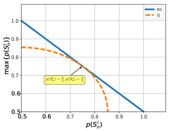
Figure 1: [color online] Plot of maximum achievable winning probability in a particular Snjsuperscriptsubscript𝑆𝑛𝑗S_{n}^{j} game, max𝒩𝒮{p(Snj)}subscript𝒩𝒮𝑝superscriptsubscript𝑆𝑛𝑗\max_{\mathcal{NS}}\{p(S_{n}^{j})\}, against the observed winning probability in another Snisuperscriptsubscript𝑆𝑛𝑖S_{n}^{i} game, p(Sni)𝑝superscriptsubscript𝑆𝑛𝑖p(S_{n}^{i}) (when Sni,Snjsuperscriptsubscript𝑆𝑛𝑖superscriptsubscript𝑆𝑛𝑗S_{n}^{i},S_{n}^{j} are not trivially complementary). For maximization over no-signaling probability distributions, the solid blue line, and for quantum probabilities, the dashed orange curve.

The relations presented in this Theorem are tight. The above relation is saturated by the convex combination of two distinct Svetlichny’s boxes (a no-signaling correlation that wins the Svetlichny’s non-local game with unit probability), specifically Snjsuperscriptsubscript𝑆𝑛𝑗S_{n}^{j}-box and Snisuperscriptsubscript𝑆𝑛𝑖S_{n}^{i}-box [see FIG. 1 blue curve]. These boxes also form the extremal points of the n𝑛n-party no-signaling polytope. When p(Snj)=1𝑝subscriptsuperscript𝑆𝑗𝑛1p(S^{j}_{n})=1, it implies that the correlation is a Snjsuperscriptsubscript𝑆𝑛𝑗S_{n}^{j}-box with p(Sni)=12𝑝superscriptsubscript𝑆𝑛𝑖12p(S_{n}^{i})=\frac{1}{2}. When p(Sni)=1𝑝subscriptsuperscript𝑆𝑖𝑛1p(S^{i}_{n})=1, it implies the correlation is a Snisuperscriptsubscript𝑆𝑛𝑖S_{n}^{i}-box with p(Snj)=12𝑝superscriptsubscript𝑆𝑛𝑗12p(S_{n}^{j})=\frac{1}{2}. It is interesting to note that it is enough to consider p(Sni)12𝑝superscriptsubscript𝑆𝑛𝑖12p(S_{n}^{i})\geq\frac{1}{2} as p(Sni)=1p(Sni)𝑝superscriptsubscript𝑆𝑛𝑖1𝑝superscriptsuperscriptsubscript𝑆𝑛𝑖p(S_{n}^{i})=1-p({S_{n}^{i}}^{\prime}); i.e., when p(Sni)<12𝑝superscriptsubscript𝑆𝑛𝑖12p(S_{n}^{i})<\frac{1}{2}, then p(Sni)12𝑝superscriptsuperscriptsubscript𝑆𝑛𝑖12p({S_{n}^{i}}^{\prime})\geq\frac{1}{2} and max𝒩𝒮{p(Snj)}=32p(Sni)subscript𝒩𝒮𝑝superscriptsubscript𝑆𝑛𝑗32𝑝superscriptsuperscriptsubscript𝑆𝑛𝑖\max_{\mathcal{NS}}\{p(S_{n}^{j})\}=\frac{3}{2}-p({S_{n}^{i}}^{\prime}). For detailed proof of this Theorem see Appendix C.. To approximate maxQ{p(Snj)}subscript𝑄𝑝superscriptsubscript𝑆𝑛𝑗\max_{Q}\{p({S_{n}^{j}})\}, we find maxQn1{p(Snj)}subscriptsubscript𝑄𝑛1𝑝superscriptsubscript𝑆𝑛𝑗\max_{Q_{n-1}}\{p({S_{n}^{j}})\} given an observed value of p(Sni)𝑝superscriptsubscript𝑆𝑛𝑖p(S_{n}^{i}), where Qn1subscript𝑄𝑛1Q_{n-1} is an convex set of correlations which approximates the quantum set of correlations. The test of whether a correlation belongs to this set or not can be formulated as a semi-definite program (SDP). Such SDPs form an ordered family, commonly referred to as the Navascues-Pironio-Acin (NPA) hierarchy Navascués et al. (2008); Wehner (2006); Vandenberghe and Boyd (1996); Liang and Doherty (2007); Doherty et al. (2008). The limit of the sequence of the ever tightening convex sets Q1Q2Q3Qmsuperset-ofsubscript𝑄1subscript𝑄2superset-ofsubscript𝑄3superset-ofsubscript𝑄𝑚Q_{1}\supset Q_{2}\supset Q_{3}\ldots\supset Q_{m} is limnQm=Qsubscript𝑛subscript𝑄𝑚𝑄\lim_{n\Rightarrow\infty}Q_{m}=Q, therefore maxQ{p(Snj)}maxQn1{p(Snj)}subscript𝑄𝑝superscriptsubscript𝑆𝑛𝑗subscriptsubscript𝑄𝑛1𝑝superscriptsubscript𝑆𝑛𝑗\max_{Q}\{p({S_{n}^{j}})\}\leq\max_{Q_{n-1}}\{p({S_{n}^{j}})\}. To plot maxQn1{p(Snj)}subscriptsubscript𝑄𝑛1𝑝superscriptsubscript𝑆𝑛𝑗\max_{Q_{n-1}}\{p({S_{n}^{j}})\} against p(Sni)𝑝superscriptsubscript𝑆𝑛𝑖p({S_{n}^{i}}), we solve a SDP for n{2,3,4,5}𝑛2345n\in\{2,3,4,5\} and obtain identical curves [see FIG. 1 orange curve]. It is interesting to note that, max𝒩𝒮{p(Snj)+p(Sni)}=maxQ{p(Snj)+p(Sni)}=32subscript𝒩𝒮𝑝superscriptsubscript𝑆𝑛𝑗𝑝superscriptsubscript𝑆𝑛𝑖subscript𝑄𝑝superscriptsubscript𝑆𝑛𝑗𝑝superscriptsubscript𝑆𝑛𝑖32\max_{\mathcal{NS}}\{p(S_{n}^{j})+p(S_{n}^{i})\}=\max_{Q}\{p(S_{n}^{j})+p(S_{n}^{i})\}=\frac{3}{2}, i.e., while the quantum curve always remains within the no-signaling curve they meet at a unique point where p(Snj)=p(Sni)=34𝑝superscriptsubscript𝑆𝑛𝑗𝑝superscriptsubscript𝑆𝑛𝑖34p(S_{n}^{j})=p(S_{n}^{i})=\frac{3}{4} [this point is highlighted in FIG. 1].
The Theorem presented above is a stepping stone to our main result presented below. Again, n𝑛n spatially separated parties share a no-signaling correlation p(u1,u2,un|x1,x2,xn)𝑝subscript𝑢1subscript𝑢2conditionalsubscript𝑢𝑛subscript𝑥1subscript𝑥2subscript𝑥𝑛p(u_{1},u_{2},\ldots u_{n}|x_{1},x_{2},\ldots x_{n}). Now if using this correlation the parties can win a n𝑛n party Svetlichny’s non-local game with a success probability p(Sni)>34𝑝superscriptsubscript𝑆𝑛𝑖34p(S_{n}^{i})>\frac{3}{4}, then the attainable success probability in any k𝑘k-party Svetlichny’s non-local game p(Skj)𝑝superscriptsubscript𝑆𝑘𝑗p(S_{k}^{j}) is upper bounded, where k<n𝑘𝑛k<n. Moreover, the upper bound decreases with the increase in p(Sni)𝑝superscriptsubscript𝑆𝑛𝑖p(S_{n}^{i}).

Theorem 2.

Sksubscript𝑆𝑘S_{k} vs. Snsubscript𝑆𝑛S_{n}: For any n𝑛n-party no-signaling correlation, there holds the following complementarity relation between the attainable winning probability in any k𝑘k-party Svetlichny’s non-local game Skjsuperscriptsubscript𝑆𝑘𝑗S_{k}^{j}, where k<n𝑘𝑛k<n, and the observed winning probability of n𝑛n party Svetlichny’s non-local game Snisuperscriptsubscript𝑆𝑛𝑖S_{n}^{i}, given by,

max𝒩𝒮{p(Skj)}={(54p(Sni)2),ifp(Sni)34,1,if12p(Sni)34,subscript𝒩𝒮𝑝superscriptsubscript𝑆𝑘𝑗cases54𝑝superscriptsubscript𝑆𝑛𝑖2if𝑝superscriptsubscript𝑆𝑛𝑖34otherwise1if12𝑝superscriptsubscript𝑆𝑛𝑖34otherwise\displaystyle\max_{\mathcal{NS}}\{p({S_{k}^{j}})\}=\begin{cases}\bigg{(}\frac{5-4p(S_{n}^{i})}{2}\bigg{)},\text{if}\ p(S_{n}^{i})\geq\frac{3}{4},\\ 1,\;\;\;\;\;\;\;\;\;\;\text{if}\ \frac{1}{2}\leq p(S_{n}^{i})\leq\frac{3}{4},\\ \end{cases}{} (16)

where SkjSni||(𝒜nk=a,nk=b)S_{k}^{j}\equiv S_{n}^{i}||(\mathcal{A}_{n-k}=a,\mathcal{B}_{n-k}=b) for some a,b{0,1}𝑎𝑏01a,b\in\{0,1\}.

Refer to caption
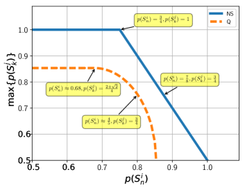
Figure 2: [color online] Plot of maximum achievable winning probability in a particular Skjsuperscriptsubscript𝑆𝑘𝑗S_{k}^{j} game, max{p(Skj)}𝑝superscriptsubscript𝑆𝑘𝑗\max\{p(S_{k}^{j})\}, against the observed winning probability in a Snisuperscriptsubscript𝑆𝑛𝑖S_{n}^{i} game, p(Sni)𝑝superscriptsubscript𝑆𝑛𝑖p(S_{n}^{i}) (when SkjSni|(𝒜nk=a,nk=b)superscriptsubscript𝑆𝑘𝑗conditionalsuperscriptsubscript𝑆𝑛𝑖formulae-sequencesubscript𝒜𝑛𝑘𝑎subscript𝑛𝑘𝑏S_{k}^{j}\equiv S_{n}^{i}|(\mathcal{A}_{n-k}=a,\mathcal{B}_{n-k}=b) for some a,b{0,1}𝑎𝑏01a,b\in\{0,1\}). For maximization over no-signaling probability distributions, the blue curve, and for quantum probabilities, the orange curve.

The Theorem states that if one witnesses genuine n𝑛n-party non-locality, i.e., p(Sn)>34𝑝subscript𝑆𝑛34p(S_{n})>\frac{3}{4}, then the no-signaling constraints imply an upper bound on the amount of attainable genuine k𝑘k-party non-locality p(Sk)𝑝subscript𝑆𝑘p(S_{k}) for any k<n𝑘𝑛k<n. The relation presented in Theorem 2. is tight when the k𝑘k-party game Skjsuperscriptsubscript𝑆𝑘𝑗S_{k}^{j} whose winning probability we are maximizing is one of the four Sksubscript𝑆𝑘S_{k}-games obtained by fixing 𝒜nk,nksubscript𝒜𝑛𝑘subscript𝑛𝑘\mathcal{A}_{n-k},\mathcal{B}_{n-k} from the n𝑛n party Snisuperscriptsubscript𝑆𝑛𝑖S_{n}^{i}-game. When p(Skj)=1𝑝superscriptsubscript𝑆𝑘𝑗1p(S_{k}^{j})=1 we have a Skjsuperscriptsubscript𝑆𝑘𝑗S_{k}^{j}-box. If we have a completely random distribution for the remaining nk𝑛𝑘n-k parties, i.e., p(uk+1,uk+2,un|xk+1,xk+2,xn)=12nk𝑝subscript𝑢𝑘1subscript𝑢𝑘2conditionalsubscript𝑢𝑛subscript𝑥𝑘1subscript𝑥𝑘2subscript𝑥𝑛1superscript2𝑛𝑘p(u_{k+1},u_{k+2},\ldots u_{n}|x_{k+1},x_{k+2},\ldots x_{n})=\frac{1}{2^{n-k}}, we have p(Sni)=12𝑝superscriptsubscript𝑆𝑛𝑖12p(S_{n}^{i})=\frac{1}{2}. However, only when the nk𝑛𝑘n-k parties have a particular deterministic distribution along with a Skjsuperscriptsubscript𝑆𝑘𝑗S_{k}^{j}-box, p(Sni)=34𝑝superscriptsubscript𝑆𝑛𝑖34p(S_{n}^{i})=\frac{3}{4}. For p(Sni)34𝑝superscriptsubscript𝑆𝑛𝑖34p(S_{n}^{i})\geq\frac{3}{4}, the curve in the relation is simply the convex combination between Skjsuperscriptsubscript𝑆𝑘𝑗S_{k}^{j}-box along-with the deterministic distribution for nk𝑛𝑘n-k parties and the Snisuperscriptsubscript𝑆𝑛𝑖S_{n}^{i}-box [see FIG. 2 blue curve]. We use the set, Qn1subscript𝑄𝑛1Q_{n-1} from NPA hierarchy, to approximate the quantum case for Sksubscript𝑆𝑘S_{k} vs. Snsubscript𝑆𝑛S_{n}. We plot maxQn1p(Skj)subscriptsubscript𝑄𝑛1𝑝superscriptsubscript𝑆𝑘𝑗\max_{Q_{n-1}}p(S_{k}^{j}) against p(Sni)𝑝superscriptsubscript𝑆𝑛𝑖p(S_{n}^{i}) for n{2,3,4,5}𝑛2345n\in\{2,3,4,5\} and k{1,2,n1}𝑘12𝑛1k\in\{1,2,\ldots n-1\} and find identical curves [see FIG. 2 orange curve]. In the quantum scenario, we find that the complementarity relations are tightened. It is interesting to note that the quantum curve always lies within the no-signaling curve and never touches it. As noted above, in the no-signaling case max𝒩𝒮{p(Skj)}subscript𝒩𝒮𝑝superscriptsubscript𝑆𝑘𝑗\max_{\mathcal{NS}}\{p(S_{k}^{j})\} decreases for p(Sni)>34𝑝superscriptsubscript𝑆𝑛𝑖34p(S_{n}^{i})>\frac{3}{4}, on the other hand in the quantum case maxQ{p(Skj)}subscript𝑄𝑝superscriptsubscript𝑆𝑘𝑗\max_{Q}\{p(S_{k}^{j})\} decreases for p(Sni)0.68greater-than-or-equivalent-to𝑝superscriptsubscript𝑆𝑛𝑖0.68p(S_{n}^{i})\gtrsim 0.68 [these points are highlighted in FIG. 2].
The proof of the above Theorem relies on the fact that, upon fixing the values of nk𝑛𝑘n-k party Boolean variables, 𝒜nksubscript𝒜𝑛𝑘\mathcal{A}_{n-k} and nksubscript𝑛𝑘\mathcal{B}_{n-k}, a Snisuperscriptsubscript𝑆𝑛𝑖S_{n}^{i} game yields four distinct Sksubscript𝑆𝑘S_{k} games. Using Property 3. and Property 4. one may write the winning probability of a Snisuperscriptsubscript𝑆𝑛𝑖S_{n}^{i} game as,

p(Sni)=𝑝superscriptsubscript𝑆𝑛𝑖absent\displaystyle p({S_{n}^{i}})={}
12(p(𝒜nk=0|nk=0)p(Sk1|𝒜nk=0,nk=0)\displaystyle\frac{1}{2}\bigg{(}p(\mathcal{A}_{n-k}=0|\mathcal{B}_{n-k}=0)p({S_{k}^{1}}|\mathcal{A}_{n-k}=0,\mathcal{B}_{n-k}=0){}
+p(𝒜nk=1|nk=0)p(Sk1|𝒜nk=1|nk=0)𝑝subscript𝒜𝑛𝑘conditional1subscript𝑛𝑘0𝑝conditionalsuperscriptsuperscriptsubscript𝑆𝑘1subscript𝒜𝑛𝑘conditional1subscript𝑛𝑘0\displaystyle+p(\mathcal{A}_{n-k}=1|\mathcal{B}_{n-k}=0)p({S_{k}^{1}}^{\prime}|\mathcal{A}_{n-k}=1|\mathcal{B}_{n-k}=0)
+p(𝒜nk=0|nk=1)p(Sk2|𝒜nk=0,nk=1)𝑝subscript𝒜𝑛𝑘conditional0subscript𝑛𝑘1𝑝formulae-sequenceconditionalsuperscriptsubscript𝑆𝑘2subscript𝒜𝑛𝑘0subscript𝑛𝑘1\displaystyle+p(\mathcal{A}_{n-k}=0|\mathcal{B}_{n-k}=1)p({S_{k}^{2}}|\mathcal{A}_{n-k}=0,\mathcal{B}_{n-k}=1){}
+p(𝒜nk=1|nk=1)p(Sk2|𝒜nk=1,nk=1)),\displaystyle+p(\mathcal{A}_{n-k}=1|\mathcal{B}_{n-k}=1)p({S_{k}^{2}}^{\prime}|\mathcal{A}_{n-k}=1,\mathcal{B}_{n-k}=1)\bigg{)},\;{}

where the conditional probability distribution p(𝒜nk|nk)𝑝conditionalsubscript𝒜𝑛𝑘subscript𝑛𝑘p(\mathcal{A}_{n-k}|\mathcal{B}_{n-k}) can be computed from the marginal probability distribution p(uk+1,uk+2un|xk+1,xk+2xn)𝑝subscript𝑢𝑘1conditionalsubscript𝑢𝑘2subscript𝑢𝑛subscript𝑥𝑘1subscript𝑥𝑘2subscript𝑥𝑛p(u_{k+1},u_{k+2}\ldots u_{n}|x_{k+1},x_{k+2}\ldots x_{n}) of nk𝑛𝑘n-k parities. Now, the above relation is obtained using the relations in Theorem 1.; i.e., by comparing p(Sk1|𝒜nk=0,nk=0)𝑝formulae-sequenceconditionalsuperscriptsubscript𝑆𝑘1subscript𝒜𝑛𝑘0subscript𝑛𝑘0p(S_{k}^{1}|\mathcal{A}_{n-k}=0,\mathcal{B}_{n-k}=0), p(Sk1|𝒜nk=1,nk=0)𝑝formulae-sequenceconditionalsuperscriptsubscript𝑆𝑘1subscript𝒜𝑛𝑘1subscript𝑛𝑘0p({S_{k}^{1}}|\mathcal{A}_{n-k}=1,\mathcal{B}_{n-k}=0), p(Sk2|𝒜nk=0,nk=1)𝑝formulae-sequenceconditionalsuperscriptsubscript𝑆𝑘2subscript𝒜𝑛𝑘0subscript𝑛𝑘1p(S_{k}^{2}|\mathcal{A}_{n-k}=0,\mathcal{B}_{n-k}=1) and p(Sk2|𝒜nk=1,nk=1)𝑝formulae-sequenceconditionalsuperscriptsuperscriptsubscript𝑆𝑘2subscript𝒜𝑛𝑘1subscript𝑛𝑘1p({S_{k}^{2}}^{\prime}|\mathcal{A}_{n-k}=1,\mathcal{B}_{n-k}=1) with the winning probability of a particular k𝑘k-party Svetlichny’s non-local game, say p(Sk1)𝑝superscriptsubscript𝑆𝑘1p(S_{k}^{1}), irrespective of the assignment of 𝒜nk,nksubscript𝒜𝑛𝑘subscript𝑛𝑘\mathcal{A}_{n-k},\mathcal{B}_{n-k} [see FIG. 3]. The actual proof of this theorem is rather arduous and can be found in Appendix E..

Refer to caption
Figure 3: The proof sketch for Theorem 2.. It utilizes the Property 3., Property 4. and the relation presented in Theorem 1..

V Relation with Monogamy of non-locality

In this section, we highlight the key differences and the subtle relationship between monogamy of non-local correlations and complementarity of genuine multipartite non-locality. It has been observed by several authors Toner (2009); Kim et al. (2009); Pawłowski and Brukner (2009); Ramanathan et al. (2012); Bai et al. (2014); Osborne and Verstraete (2006); Koashi and Winter (2004); Hiroshima et al. (2007), that a system being (non-locally) correlated with another one, cannot have arbitrarily high non-local correlation with a third system: this has been dubbed as the ‘monogamous’ nature of non-locality. For instance, non-local correlations between spatially separated systems that lead to the violation of the well-known CHSH inequality (6), exhibit this phenomenon. It was later shown that all no-signaling correlations violating any Bell-type inequality exhibit monogamy Pawłowski and Brukner (2009). This feature of non-local correlations, imposed by the no-signaling condition reflects the monogamy of entanglement under the much stricter quantum constraints. Furthermore, this feature is significant in various cryptographic scenarios, where two parties A1subscript𝐴1A_{1} and A2subscript𝐴2A_{2} can verify a sufficient amount of non-locality to guarantee that their systems are not correlated with any eavesdropper’s system Toner (2009).
Consider the case of three spatially separated parties A1,A2,A3subscript𝐴1subscript𝐴2subscript𝐴3A_{1},A_{2},A_{3}, sharing a no-signaling correlation p(u1,u2,u3|x1,x2,x3)𝑝subscript𝑢1subscript𝑢2conditionalsubscript𝑢3subscript𝑥1subscript𝑥2subscript𝑥3p(u_{1},u_{2},u_{3}|x_{1},x_{2},x_{3}). It was first shown by Toner Toner (2009), that in a Bell experiment with three spatially separated parties A1,A2,A3subscript𝐴1subscript𝐴2subscript𝐴3A_{1},A_{2},A_{3}, when A1,A2subscript𝐴1subscript𝐴2A_{1},A_{2} observe the violation of the CHSH inequality, then the no-signaling condition imposes that there can be no violation of the CHSH inequality between A1,A3subscript𝐴1subscript𝐴3A_{1},A_{3}. This is conveniently captured by the following ‘monogamy’ relation:

max𝒩𝒮{pA1,A2(S2)+pA1,A3(S2)}subscript𝒩𝒮subscript𝑝subscript𝐴1subscript𝐴2subscript𝑆2subscript𝑝subscript𝐴1subscript𝐴3subscript𝑆2\displaystyle\max_{\mathcal{NS}}\{p_{A_{1},A_{2}}(S_{2})+p_{A_{1},A_{3}}(S_{2})\} =2maxLV{p(S2)}absent2subscript𝐿𝑉𝑝subscript𝑆2\displaystyle=2\max_{LV}\{p(S_{2})\} (18)
=32,absent32\displaystyle=\frac{3}{2},

where pA1,A2(S2)=u3S2p(u1,u2,u3|x1,x2,x3)subscript𝑝subscript𝐴1subscript𝐴2subscript𝑆2subscriptsubscript𝑢3subscriptsubscript𝑆2𝑝subscript𝑢1subscript𝑢2conditionalsubscript𝑢3subscript𝑥1subscript𝑥2subscript𝑥3p_{A_{1},A_{2}}(S_{2})=\sum_{u_{3}}\sum_{S_{2}}p(u_{1},u_{2},u_{3}|x_{1},x_{2},x_{3}) and pA1,A3(S2)subscript𝑝subscript𝐴1subscript𝐴3subscript𝑆2p_{A_{1},A_{3}}(S_{2}) is similarly defined. This relation is saturated for no-signaling constraints for all possible values of pA1,A2(S2),pA1,A3(S2)subscript𝑝subscript𝐴1subscript𝐴2subscript𝑆2subscript𝑝subscript𝐴1subscript𝐴3subscript𝑆2p_{A_{1},A_{2}}(S_{2}),p_{A_{1},A_{3}}(S_{2}) [see FIG. 6a curve for p(S3)=0.75𝑝subscript𝑆30.75p(S_{3})=0.75 ]. Interestingly, the same relation holds for quantum case as well. However, for the quantum case it is saturated only for pA1,A2(S2)=34,pA1,A3(S2)=34formulae-sequencesubscript𝑝subscript𝐴1subscript𝐴2subscript𝑆234subscript𝑝subscript𝐴1subscript𝐴3subscript𝑆234p_{A_{1},A_{2}}(S_{2})=\frac{3}{4},p_{A_{1},A_{3}}(S_{2})=\frac{3}{4} [see FIG. 6b curve for p(S3)=0.675𝑝subscript𝑆30.675p(S_{3})=0.675] .
The complementarity relations for this tripartite system are,

max𝒩𝒮{pA1A2(S2)}={(54p(S3)2),ifp(S3)34,1,if12p(S3i)34,subscript𝒩𝒮subscript𝑝subscript𝐴1subscript𝐴2subscript𝑆2cases54𝑝subscript𝑆32if𝑝subscript𝑆334otherwise1if12𝑝superscriptsubscript𝑆3𝑖34otherwise\displaystyle\max_{\mathcal{NS}}\{p_{A_{1}A_{2}}({S_{2}})\}=\begin{cases}\bigg{(}\frac{5-4p(S_{3})}{2}\bigg{)},\text{if}\ p(S_{3})\geq\frac{3}{4},\\ 1,\;\;\;\;\;\;\;\;\;\;\text{if}\ \frac{1}{2}\leq p(S_{3}^{i})\leq\frac{3}{4},\\ \end{cases}{} (19)

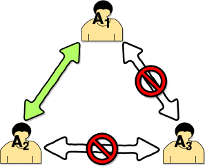
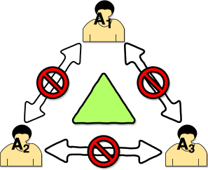
and exactly same for max𝒩𝒮{pA1A3(S2)}subscript𝒩𝒮subscript𝑝subscript𝐴1subscript𝐴3subscript𝑆2\max_{\mathcal{NS}}\{p_{A_{1}A_{3}}({S_{2}})\}. In general the monogamy relations do not take into account the amount of genuine multipartite non-locality the system may have and are tight only under the assumption that there isn’t any as is the case with the relation in (18). For a multipartite system, the monogamy relations reveal that if a high degree of (genuine n𝑛n-party) non-local correlation is observed in a system of n𝑛n-parties then none of these n𝑛n-parties can be highly correlated with any other external party. While on the other hand the complementarity relations presented in this work, on the other hand, deal with the distribution of genuine non-locality within a n𝑛n-party system; i.e., they do not take any external parties into consideration (see FIG. 4 for the visualization of the difference in the notions).
Refer to caption
(a) Monogamy of non-locality.
Refer to caption
(b) Complementarity of genuine tripartite and bipartite non-locality.
Figure 4: [color online] Extremal form of monogamy of non-locality vs. extremal form of complimentarity of genuine non-locality in a tripartite scenario.

While these two features of no-signaling non-theories are distinct, they are subtly related. In particular, the monogamy relation, (18), tightens with increasing presence of genuine multipartite non-locality. This is captured in the following modified monogamy relation,

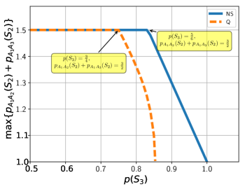
max𝒩𝒮{pA1A2(S2)+pA1A3(S2)}={43p(S3),ifp(S3)56,32,if12p(S3i)56.subscript𝒩𝒮subscript𝑝subscript𝐴1subscript𝐴2subscript𝑆2subscript𝑝subscript𝐴1subscript𝐴3subscript𝑆2cases43𝑝subscript𝑆3if𝑝subscript𝑆356otherwise32if12𝑝superscriptsubscript𝑆3𝑖56otherwise\max_{\mathcal{NS}}\{p_{A_{1}A_{2}}({S_{2}})+p_{A_{1}A_{3}}({S_{2}})\}\\ =\begin{cases}4-3p(S_{3}),~{}~{}~{}\text{if}\ p(S_{3})\geq\frac{5}{6},\\ \frac{3}{2},~{}\;\;\;\;\;\;\;\;\;~{}~{}~{}~{}~{}~{}\text{if}\ \frac{1}{2}\leq p(S_{3}^{i})\leq\frac{5}{6}.\end{cases}{} (20)

Notice that the complementarity relations of the type (19) do not imply the monogamy relation (20) on their own; i.e., one does not arrive at the above result just by adding such complementarity relations for different pairs of parties, i.e., max𝒩𝒮{pA1A2(S2)}+max𝒩𝒮{pA1A3(S2)}max𝒩𝒮{pA1A2(S2)+pA1A3(S2)}not-equivalent-tosubscript𝒩𝒮subscript𝑝subscript𝐴1subscript𝐴2subscript𝑆2subscript𝒩𝒮subscript𝑝subscript𝐴1subscript𝐴3subscript𝑆2subscript𝒩𝒮subscript𝑝subscript𝐴1subscript𝐴2subscript𝑆2subscript𝑝subscript𝐴1subscript𝐴3subscript𝑆2\max_{\mathcal{NS}}\{p_{A_{1}A_{2}}(S_{2})\}+\max_{\mathcal{NS}}\{p_{A_{1}A_{3}}(S_{2})\}\not\equiv\max_{\mathcal{NS}}\{p_{A_{1}A_{2}}(S_{2})+p_{A_{1}A_{3}}(S_{2})\}. Interestingly, the maximum value of the sum max𝒩𝒮{pA1A2(S2)+pA1A3(S2)}subscript𝒩𝒮subscript𝑝subscript𝐴1subscript𝐴2subscript𝑆2subscript𝑝subscript𝐴1subscript𝐴3subscript𝑆2\max_{\mathcal{NS}}\{p_{A_{1}A_{2}}(S_{2})+p_{A_{1}A_{3}}(S_{2})\} remains constant at 3232\frac{3}{2} for 12p(S3)5612𝑝subscript𝑆356\frac{1}{2}\leq p(S_{3})\leq\frac{5}{6} and decreases for p(S3)>56𝑝subscript𝑆356p(S_{3})>\frac{5}{6} [see FIG. 5 blue curve]. We use SDP once again to approximate the quantum case. Here the maximum value of the sum maxQ{pA1A2(S2)+pA1A3(S2)}subscript𝑄subscript𝑝subscript𝐴1subscript𝐴2subscript𝑆2subscript𝑝subscript𝐴1subscript𝐴3subscript𝑆2\max_{Q}\{p_{A_{1}A_{2}}(S_{2})+p_{A_{1}A_{3}}(S_{2})\} remains constant at 3232\frac{3}{2} for 12p(S3)3412𝑝subscript𝑆334\frac{1}{2}\leq p(S_{3})\leq\frac{3}{4} and decreases for p(S3)>34𝑝subscript𝑆334p(S_{3})>\frac{3}{4} [see FIG. 5 orange curve]. The above result can easily be proved using exactly the same proof structure used for Theorem 2..
Refer to caption
Figure 5: [color online] Plot of maximum achievable value of the sum of winning probabilities of a S2subscript𝑆2S_{2} game played between A1,A2subscript𝐴1subscript𝐴2A_{1},A_{2} and A1,A3subscript𝐴1subscript𝐴3A_{1},A_{3}, max{pA1A2(S2)+pA1A3(S2)}subscript𝑝subscript𝐴1subscript𝐴2subscript𝑆2subscript𝑝subscript𝐴1subscript𝐴3subscript𝑆2\max\{p_{A_{1}A_{2}}(S_{2})+p_{A_{1}A_{3}}(S_{2})\}, against the observed winning probability in a S3subscript𝑆3S_{3} game, p(S3)𝑝subscript𝑆3p(S_{3}). For maximization over no-signaling probability distributions, the solid blue line, and for quantum probabilities, the dashed orange curve.

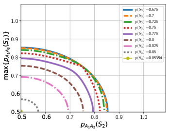
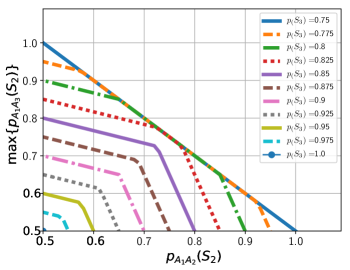
However, the above relation does not capture the delicate details involved in this scenario. Observe that in the above relation the maximal value of the sum max𝒩𝒮{pA1A2(S2)+pA1A3(S2)}subscript𝒩𝒮subscript𝑝subscript𝐴1subscript𝐴2subscript𝑆2subscript𝑝subscript𝐴1subscript𝐴3subscript𝑆2\max_{\mathcal{NS}}\{p_{A_{1}A_{2}}(S_{2})+p_{A_{1}A_{3}}(S_{2})\} decreases only after p(S3)>56𝑝subscript𝑆356p(S_{3})>\frac{5}{6}. On the other hand, the maximal possible values of the individual terms max𝒩𝒮{pA1,A2(S2)}subscript𝒩𝒮subscript𝑝subscript𝐴1subscript𝐴2subscript𝑆2\max_{\mathcal{NS}}\{p_{A_{1},A_{2}}(S_{2})\} and max𝒩𝒮{pA1,A3(S2)}subscript𝒩𝒮subscript𝑝subscript𝐴1subscript𝐴3subscript𝑆2\max_{\mathcal{NS}}\{p_{A_{1},A_{3}}(S_{2})\} decrease all the way from p(S3)34𝑝subscript𝑆334p(S_{3})\geq\frac{3}{4}. In order to help visualize this, we plot max𝒩𝒮{pA1,A2(S2)}subscript𝒩𝒮subscript𝑝subscript𝐴1subscript𝐴2subscript𝑆2\max_{\mathcal{NS}}\{p_{A_{1},A_{2}}(S_{2})\} against pA1,A3(S2)subscript𝑝subscript𝐴1subscript𝐴3subscript𝑆2p_{A_{1},A_{3}}(S_{2}) given different observed values of p(S3)𝑝subscript𝑆3p(S_{3}) [see FIG. 6a]. For p(S3)[34,56]𝑝subscript𝑆33456p(S_{3})\in[\frac{3}{4},\frac{5}{6}] the maximum sum is still 3232\frac{3}{2}, however the individual maximums continually decrease, giving the plots a plateau like shape. Again a similar trend is observed under the quantum constraints. We plot maxQ{pA1,A2(S2)}subscript𝑄subscript𝑝subscript𝐴1subscript𝐴2subscript𝑆2\max_{Q}\{p_{A_{1},A_{2}}(S_{2})\} against pA1,A3(S2)subscript𝑝subscript𝐴1subscript𝐴3subscript𝑆2p_{A_{1},A_{3}}(S_{2}) given different observed values of p(S3)𝑝subscript𝑆3p(S_{3}) [see FIG. 6b]. For p(S3)[0.68,34]𝑝subscript𝑆30.6834p(S_{3})\in[0.68,\frac{3}{4}] the maximum sum is still 3232\frac{3}{2}, however the individual maximums continually decrease, giving the plots a non-trivial shape.
Refer to caption
(a) No-signaling
Refer to caption
(b) Quantum
Figure 6: [color online] The curves of maximum achievable success probability in a S2subscript𝑆2S_{2} game, played between A1,A2subscript𝐴1subscript𝐴2A_{1},A_{2}, max{pA1,A2(S2)}subscript𝑝subscript𝐴1subscript𝐴2subscript𝑆2\max\{p_{A_{1},A_{2}}(S_{2})\}, against the winning probability in a S2subscript𝑆2S_{2} game, played between A1,A3subscript𝐴1subscript𝐴3A_{1},A_{3}, pA1,A3(S2)subscript𝑝subscript𝐴1subscript𝐴3subscript𝑆2p_{A_{1},A_{3}}(S_{2}), given different observed value of the winning probability in a S3subscript𝑆3S_{3} game, pA1,A2,A3(S3)subscript𝑝subscript𝐴1subscript𝐴2subscript𝐴3subscript𝑆3p_{A_{1},A_{2},A_{3}}(S_{3}). The first curve from the top corresponds to the top most legend entry, the second curve to the second legend entry and so on.

VI Conclusions and future directions

This work is an attempt to capture a characteristic feature of Nature, namely, when a system of multiple particles (say spin-1212\frac{1}{2} particles) manifests genuine non-local correlation, then there cannot be arbitrarily high non-local correlation among any subset of particles. We refer to this feature, as the complementarity of genuine multipartite non-locality. We bring forth this feature without invoking the particulars of the quantum theory. Instead, we show that any no-signaling non-local theory will manifest this property. We use the Svetlichny’s criterion for genuine multipartite non-locality and Svetlichny’s family of non-local games, to showcase this feature. Svetlichny’s non-local games have a recursive structure; i.e., a Svetlichny’s non-local game for n𝑛n parties yields four distinct Svetlichny’s non-local games for k𝑘k parties upon conditioning over inputs and outputs of the nk𝑛𝑘n-k parties [see FIG. 3]. We exploit this feature in-order to prove our main results (15),(16) for the no-signaling constraints. Our numerical analysis reveals the fact that these relations tighten under the much stricter quantum constraints [see FIG. 1 and 2].
However, this feature of no-signaling non-local theories is not restricted to any particular framework. Also, Svetlichny’s criterion provides only a sufficient condition for genuine multipartite non-locality. Therefore, for completeness, we provide numerical evidence showcasing this property, by plotting max𝒩𝒮(p(S2)),maxQ(p(S2))subscript𝒩𝒮𝑝subscript𝑆2subscript𝑄𝑝subscript𝑆2\max_{\mathcal{NS}}(p(S_{2})),\max_{Q}(p(S_{2})) (where S2subscript𝑆2S_{2} is the non-local game equivalent to well known CHSH-expression) against several tripartite measures of non-locality [see Appendix A.].
We compare the notions of complementarity of genuine multipartite non-locality and monogamy of non-locality. While monogamy of non-locality entails a restriction on possible non-local correlations of an external party with any particular party (or a bunch of parties) within a (genuinely non-locally) correlated system, the notion of complementarity of genuine multipartite non-locality on the other hand deals with distribution of genuine non-local correlation within a system having some overall genuine correlation [see FIG. 4]. While these are distinct features of no-signaling non-local theories, they are subtly related. As a bi-product of this comparison, we find that the monogamy relations tighten with increase in genuine multipartite non-locality for both the no-signaling and the quantum constraints (20)[see FIG. 5 and 6].
Apart from the straightforward relevance to the field of foundations, the complementarity relations presented here have potential applications to the fields of communication complexity, cryptography and game theory. It was shown that for a very large class of multipartite Bell-type inequalities, correlations which violate them lead to an advantage in corresponding communication complexity protocols Brukner et al. (2004). And in-turn this advantage in communication complexity protocols is directly related to security of cryptographic protocols Becker and Wille (1998); Micciancio and Panjwani (2004); Guedes and de Assis (2011). In particular, in protocols involving multiple parties, where the success of the protocol is directly related to amount of violation of genuine multipartite non-locality testing Bell-type inequalities, the complementarity relations provide security against a conspiring (cheating) subgroup of parties.
In this work, we deal with how the amount genuine multipartite non-locality of one (arbitrary) subset is restricted due to presence of genuine multipartite non-locality in the system as a whole. It would be interesting to further study the distribution of genuine multipartite non-locality among multiple (disjoint or overlapping) subsets given the presence of genuine multipartite non-locality in the system as a whole.

VII Acknowledgements

AC would like to thank Dr. G Kar, Dr M Banik of PAMU, ISI, Kolkata, India for intuitive advice and D Saha, Dr. M Pawłowski and Dr. K Horodecki of KCIK, Gdansk, Poland for detailed discussions. This project was partly supported by grant, Harmonia 4 (Grant number: UMO-2013/08/M/ST2/00626), ERC AdG QOLAPS.

References

Here we provide a brief map of our Appendices. In Appendix A, we provide numerical evidence for our main result, by plotting max𝒩𝒮{p(S2)},maxQ{p(S2)}subscript𝒩𝒮𝑝subscript𝑆2subscript𝑄𝑝subscript𝑆2\max_{\mathcal{NS}}\{p(S_{2})\},\max_{{Q}}\{p(S_{2})\} against observed values of an assorted bunch of tripartite non-locality measures. Appendix B contains the proof for Property 3. and Property 4.. Appendix C, contains the proof for Theorem 1.. Appendix D, contains derivation of complementary relations between the winning probability of a S2subscript𝑆2S_{2} game vs. single party marginals and of a Snsubscript𝑆𝑛S_{n} game vs. single party marginals and nk𝑛𝑘n-k party marginals. Appendix E, contains the proof of Theorem 2.

Appendix A Other tripartite measures of non-locality vs. CHSH

In this section, we provide numerical evidence for complementarity between tripartite genuine non-locality and bipartite non-locality using a selected bunch of tripartite measures and p(S2)𝑝subscript𝑆2p(S_{2}) as the bipartite measure of non-locality. Let us suppose, that a tripartite non-locality measure, 𝒞3subscript𝒞3\mathcal{C}_{3} has an observed value c𝑐c. Now, given this fact, we wish to find max𝒩𝒮p(S2)subscript𝒩𝒮𝑝subscript𝑆2\max_{\mathcal{NS}}p(S_{2}) and approximate maxQp(S2)subscript𝑄𝑝subscript𝑆2\max_{Q}p(S_{2}). Now, notice that the no-signaling constraints are linear on the conditional probabilities, hence, we solve the linear program of the form,

maximize p(S2)𝑝subscript𝑆2\displaystyle p(S_{2})
subject to 𝒞3=c,subscript𝒞3𝑐\displaystyle\mathcal{C}_{3}=c,
p(u1,u2,u3|x1,x2,x3)𝒩𝒮.𝑝subscript𝑢1subscript𝑢2conditionalsubscript𝑢3subscript𝑥1subscript𝑥2subscript𝑥3𝒩𝒮\displaystyle p(u_{1},u_{2},u_{3}|x_{1},x_{2},x_{3})\in{\mathcal{NS}}.

Furthermore, we approximate using Q2subscript𝑄2Q_{2}, a convex set of correlations, which approximates the quantum correlations. Its testing condition is a SDP program in the NPA hierarchy,

maximize p(S2)𝑝subscript𝑆2\displaystyle p(S_{2})
subject to 𝒞3=c,subscript𝒞3𝑐\displaystyle\mathcal{C}_{3}=c,
p(u1,u2,u3|x1,x2,x3)Q2.𝑝subscript𝑢1subscript𝑢2conditionalsubscript𝑢3subscript𝑥1subscript𝑥2subscript𝑥3subscript𝑄2\displaystyle p(u_{1},u_{2},u_{3}|x_{1},x_{2},x_{3})\in{Q}_{2}.

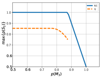
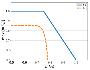
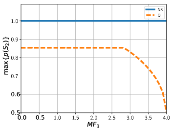
We use two variations of Svetlichny’s non-local game, M3,N3subscript𝑀3subscript𝑁3M_{3},N_{3} Barrett et al. (2005); Pironio et al. (2011). These differ from each-other and from S3subscript𝑆3S_{3} in the way the inputs, x1,x2,x3subscript𝑥1subscript𝑥2subscript𝑥3x_{1},x_{2},x_{3}, are included the boolean condition for success. In both cases, complementarity relations are witnessed [see FIG. 7a,7b]. Next up, we use the Mermin’s tripartite expression, MF3𝑀subscript𝐹3MF_{3}. It is a Bell-type (CHSH like) expression, with local-real bound, maxLV{MF3}=2subscript𝐿𝑉𝑀subscript𝐹32\max_{LV}\{MF_{3}\}=2 equal no-signaling and quantum upper bounds, max𝒩𝒮{MF3}=maxQ{MF3}=subscript𝒩𝒮𝑀subscript𝐹3subscript𝑄𝑀subscript𝐹3absent\max_{\mathcal{NS}}\{MF_{3}\}=\max_{Q}\{MF_{3}\}=. As discussed earlier, the violation of Mermin’s inequality does not imply genuine multipartite non-locality, but just non-locality. As a result the characteristic complementarity is witnessed in the case of much tighter quantum constraints, no complementarity is witnessed at all in the case of no-signaling constraints [see FIG. 7c].
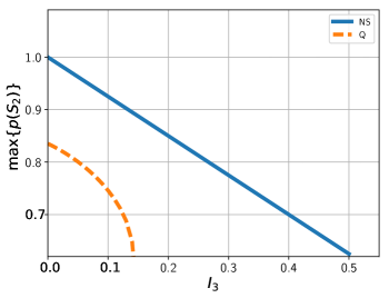
The correlations which can not be represented as in the form given in (II.2), are referred to as genuinely tripartite SV2𝑆subscript𝑉2SV_{2} non-local. While prescribing, (II.2), Svetlichny tacitly assumed that the measurements can be regarded as simultaneous or the probabilities pλ1(u1,u2|x1x2),pλ2(x2x3|X2X3),pλ3(u1,u3|x1,x3)subscript𝑝subscript𝜆1subscript𝑢1conditionalsubscript𝑢2subscript𝑥1subscript𝑥2subscript𝑝subscript𝜆2conditionalsubscript𝑥2subscript𝑥3subscript𝑋2subscript𝑋3subscript𝑝subscript𝜆3subscript𝑢1conditionalsubscript𝑢3subscript𝑥1subscript𝑥3p_{{\lambda}_{1}}(u_{1},u_{2}|x_{1}x_{2}),p_{\lambda_{2}}(x_{2}x_{3}|X_{2}X_{3}),p_{\lambda_{3}}(u_{1},u_{3}|x_{1},x_{3}) are independent of the timing of the measurements. This assumption goes well in the case, when the hidden variables are no signaling, otherwise, one might be faced with causality paradoxes. The polytope obtained using no-signaling hidden variables is referred to as 𝒩𝒮2𝒩subscript𝒮2\mathcal{NS}_{2}. An alternative solution to the causality puzzle is provided introducing the concept of time ordering in (II.2). The corresponding polytope obtained in this case is called T2subscript𝑇2T_{2}. It should be emphasized that 𝒩𝒮2T2SV2𝒩subscript𝒮2subscript𝑇2𝑆subscript𝑉2\mathcal{NS}_{2}\subset T_{2}\subset SV_{2} where the inclusion is strict. We compare p(S2)𝑝subscript𝑆2p(S_{2}) with the probabilistic expression, I3subscript𝐼3I_{3}. The violation of the corresponding inequality, implies that the correlations are 𝒩𝒮2𝒩subscript𝒮2\mathcal{NS}_{2} and T2subscript𝑇2T_{2} non-local. Thus, I30subscript𝐼30I_{3}\leq 0 is a weaker (less stricter) inequality compared to the Svetlichny’s inequality Bancal et al. (2013). Here, the complementarity is witnessed all the way from I3>0subscript𝐼30I_{3}>0 under both no-signaling and quantum constraints [see FIG. 7d].
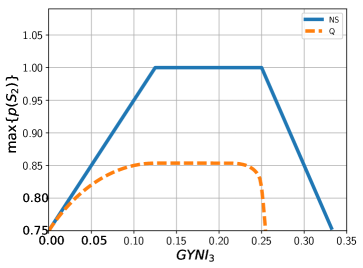
Finally, we use the guess your neighbor’s input game (GYNIn𝐺𝑌𝑁subscript𝐼𝑛GYNI_{n}) Acín et al. (2016); Pironio et al. (2011). This game consists of n𝑛n players, arranged on a ring, wherein each player receives a binary input xisubscript𝑥𝑖x_{i} for i{1,n}𝑖1𝑛i\in\{1,\ldots n\}. The aim of the game is, to obtain a situation, wherein each player outputs a bit uisubscript𝑢𝑖u_{i} equal to the input bit of it’s right neighbor, ui=xi1subscript𝑢𝑖subscript𝑥𝑖1u_{i}=x_{i-1}. In case of 333 players, the game is denoted as, GYNI3𝐺𝑌𝑁subscript𝐼3GYNI_{3}. Here again, one can clearly visualize the complementarity relations [see FIG. 7e]. The expressions for these measures, their respective quantum and no-signaling bounds are presented in the Table 1. The plots for complementarity relations can be found in FIG. 7.

Tripartite Measure Expression Quantum bound No-signaling bound
M3subscript𝑀3M_{3} u1u2u3=x1x2x3direct-sumsubscript𝑢1subscript𝑢2subscript𝑢3subscript𝑥1subscript𝑥2subscript𝑥3u_{1}\oplus u_{2}\oplus u_{3}=x_{1}x_{2}x_{3} 7878\frac{7}{8} 1
N3subscript𝑁3N_{3} u1u2u3=x1x2x2x3direct-sumsubscript𝑢1subscript𝑢2subscript𝑢3direct-sumsubscript𝑥1subscript𝑥2subscript𝑥2subscript𝑥3u_{1}\oplus u_{2}\oplus u_{3}=x_{1}x_{2}\oplus x_{2}x_{3} 0.7818absent0.7818\approx 0.7818 1
MF3𝑀subscript𝐹3MF_{3}   x1=1,x2=0,x3=0+x1=0,x2=1,x3=0delimited-⟨⟩formulae-sequencesubscript𝑥11formulae-sequencesubscript𝑥20subscript𝑥30delimited-⟨⟩formulae-sequencesubscript𝑥10formulae-sequencesubscript𝑥21subscript𝑥30\langle x_{1}=1,x_{2}=0,x_{3}=0\rangle+\langle x_{1}=0,x_{2}=1,x_{3}=0\rangle +x1=0,x2=0,x3=1x1=0,x2=1,x3=1delimited-⟨⟩formulae-sequencesubscript𝑥10formulae-sequencesubscript𝑥20subscript𝑥31delimited-⟨⟩formulae-sequencesubscript𝑥10formulae-sequencesubscript𝑥21subscript𝑥31+\langle x_{1}=0,x_{2}=0,x_{3}=1\rangle-\langle x_{1}=0,x_{2}=1,x_{3}=1\rangle 4 4
I3subscript𝐼3I_{3}  2pA1A2(u1=0,u2=0|x1=1,x2=1)-2p_{A_{1}A_{2}}(u_{1}=0,u_{2}=0|x_{1}=1,x_{2}=1) 2pA2A3(u2=0,u3=0|x2=1,x3=1)-2p_{A_{2}A_{3}}(u_{2}=0,u_{3}=0|x_{2}=1,x_{3}=1) 2pA3A1(u3=0,u1=0|x3=1,x1=1)-2p_{A_{3}A_{1}}(u_{3}=0,u_{1}=0|x_{3}=1,x_{1}=1) p(u1=0,u2=0,u3=0|x1=0,x2=0,x3=1)-p(u_{1}=0,u_{2}=0,u_{3}=0|x_{1}=0,x_{2}=0,x_{3}=1) p(u1=0,u2=0,u3=0|x1=0,x2=1,x3=0)-p(u_{1}=0,u_{2}=0,u_{3}=0|x_{1}=0,x_{2}=1,x_{3}=0) p(u1=0,u2=0,u3=0|x1=1,x2=0,x3=0)-p(u_{1}=0,u_{2}=0,u_{3}=0|x_{1}=1,x_{2}=0,x_{3}=0) +2p(u1=0,u2=0,u3=0|x1=0,x2=1,x3=1)+2p(u_{1}=0,u_{2}=0,u_{3}=0|x_{1}=0,x_{2}=1,x_{3}=1) +2p(u1=0,u2=0,u3=0|x1=1,x2=0,x3=1)+2p(u_{1}=0,u_{2}=0,u_{3}=0|x_{1}=1,x_{2}=0,x_{3}=1) +2p(u1=0,u2=0,u3=0|x1=1,x2=1,x3=0)+2p(u_{1}=0,u_{2}=0,u_{3}=0|x_{1}=1,x_{2}=1,x_{3}=0) +2p(u1=0,u2=0,u3=0|x1=1,x2=1,x3=1)+2p(u_{1}=0,u_{2}=0,u_{3}=0|x_{1}=1,x_{2}=1,x_{3}=1) 0.14 0.5
p(GYNI3)𝑝𝐺𝑌𝑁subscript𝐼3p(GYNI_{3})   p(u1=0,u2=0,u3=0|x1=0,x2=0,x3=0)p(u_{1}=0,u_{2}=0,u_{3}=0|x_{1}=0,x_{2}=0,x_{3}=0) +p(u1=1,u2=1,u3=0|x1=0,x2=1,x3=1)+p(u_{1}=1,u_{2}=1,u_{3}=0|x_{1}=0,x_{2}=1,x_{3}=1) +p(u1=0,u2=1,u3=1|x1=1,x2=0,x3=1)+p(u_{1}=0,u_{2}=1,u_{3}=1|x_{1}=1,x_{2}=0,x_{3}=1) +p(u1=1,u2=0,u3=1|x1=1,x2=1,x3=0)+p(u_{1}=1,u_{2}=0,u_{3}=1|x_{1}=1,x_{2}=1,x_{3}=0) 0.25 1313\frac{1}{3}
Table 1: Expressions for tripartite measures of non-locality, and their corresponding quantum and no-signaling upper bounds.
Refer to caption
(a) The observed winning probability in the M3subscript𝑀3M_{3} game, p(M3)𝑝subscript𝑀3p(M_{3}).
Refer to caption
(b) The observed winning probability in the N3subscript𝑁3N_{3} game, p(N3)𝑝subscript𝑁3p(N_{3}).
Refer to caption
(c) The observed value of Mermin’s facet expression, MF3𝑀subscript𝐹3MF_{3}.
Refer to caption
(d) The observed value of I3subscript𝐼3I_{3}.
Refer to caption
(e) The observed winning probability in the GYNI game, p(GYNI3)𝑝𝐺𝑌𝑁subscript𝐼3p(GYNI_{3}).
Figure 7: Plot of maximum achievable winning probability in a S2subscript𝑆2S_{2} game, max{p(S2)}𝑝subscript𝑆2\max\{p(S_{2})\} against some tripartite measures of non-locality. For maximization over no-signaling probability distributions, the solid blue line, and for quantum probabilities, the dashed orange curve.

Appendix B Decomposition of Snsubscript𝑆𝑛S_{n}-games

A n𝑛n-party Svetlichny’s non-local game, Snisuperscriptsubscript𝑆𝑛𝑖S_{n}^{i}, reduces to four n1𝑛1n-1-party Svetlichny’s non-local games, given the fixed assignment of the input and output bits of the n𝑛nth party, denoted by Sn1jSni|(un=un,xn=xn)superscriptsubscript𝑆𝑛1𝑗conditionalsuperscriptsubscript𝑆𝑛𝑖formulae-sequencesubscript𝑢𝑛superscriptsubscript𝑢𝑛subscript𝑥𝑛superscriptsubscript𝑥𝑛S_{n-1}^{j}\equiv S_{n}^{i}|(u_{n}=u_{n}^{\prime},x_{n}=x_{n}^{\prime}), for un,xn{0,1}superscriptsubscript𝑢𝑛superscriptsubscript𝑥𝑛01u_{n}^{\prime},x_{n}^{\prime}\in\{0,1\}. Similarly, a Snjsuperscriptsubscript𝑆𝑛𝑗S_{n}^{j} game reduces to four k𝑘k-party Svetlichny’s non-local games, given the fixed assignment of the input and output bits of nk𝑛𝑘n-k parties, denoted by SkjSni|(uk+1=uk+1,un=un,xk+1=xk+1,xn=xn)superscriptsubscript𝑆𝑘𝑗conditionalsuperscriptsubscript𝑆𝑛𝑖formulae-sequencesubscript𝑢𝑘1superscriptsubscript𝑢𝑘1formulae-sequencesubscript𝑢𝑛superscriptsubscript𝑢𝑛formulae-sequencesubscript𝑥𝑘1superscriptsubscript𝑥𝑘1subscript𝑥𝑛superscriptsubscript𝑥𝑛S_{k}^{j}\equiv S_{n}^{i}|(u_{k+1}=u_{k+1}^{\prime},\ldots u_{n}=u_{n}^{\prime},x_{k+1}=x_{k+1}^{\prime},\ldots x_{n}=x_{n}^{\prime}) where ui,xi{0,1}superscriptsubscript𝑢𝑖superscriptsubscript𝑥𝑖01u_{i}^{\prime},x_{i}^{\prime}\in\{0,1\} for k<in𝑘𝑖𝑛k<i\leq n. If Snisuperscriptsubscript𝑆𝑛𝑖S_{n}^{i} game is of the form (10), then the Skjsuperscriptsubscript𝑆𝑘𝑗S_{k}^{j} game, thus obtained, is given by,

(1ikui)(k<inui)c0=\displaystyle(\bigoplus_{1\leq i\leq k}u_{i})\oplus(\bigoplus_{k<i\leq n}u_{i}{{}^{\prime}})\oplus c_{0}={}
(1i<jkxixj)(1ik(k<jnxjci)xi)(k<incixi).\displaystyle(\bigoplus_{1\leq i<j\leq k}x_{i}x_{j})\oplus(\bigoplus_{1\leq i\leq k}(\bigoplus_{k<j\leq n}x_{j}{{}^{\prime}}\oplus c_{i})\ x_{i})\oplus(\bigoplus_{k<i\leq n}c_{i}x_{i}{{}^{\prime}})\;.{}

Using the definitions of 𝒜nk,nksubscript𝒜𝑛𝑘subscript𝑛𝑘\mathcal{A}_{n-k},\mathcal{B}_{n-k}, we can rewrite the above as,

Sk1Snj|(𝒜nk=0,nk=0)superscriptsubscript𝑆𝑘1conditionalsuperscriptsubscript𝑆𝑛𝑗formulae-sequencesubscript𝒜𝑛𝑘0subscript𝑛𝑘0absent\displaystyle S_{k}^{1}\equiv S_{n}^{j}|(\mathcal{A}_{n-k}=0,\mathcal{B}_{n-k}=0)\equiv{}
1ikuic0=(1i<jkxixj)(1ikcixi),direct-sumsubscriptdirect-sum1𝑖𝑘subscript𝑢𝑖subscript𝑐0direct-sumsubscriptdirect-sum1𝑖𝑗𝑘subscript𝑥𝑖subscript𝑥𝑗subscriptdirect-sum1𝑖𝑘subscript𝑐𝑖subscript𝑥𝑖\displaystyle\bigoplus_{1\leq i\leq k}u_{i}\oplus c_{0}=(\bigoplus_{1\leq i<j\leq k}x_{i}x_{j})\oplus(\bigoplus_{1\leq i\leq k}c_{i}x_{i}){}\;,
Sk1Snj|(𝒜nk=1,nk=0)superscriptsuperscriptsubscript𝑆𝑘1conditionalsuperscriptsubscript𝑆𝑛𝑗formulae-sequencesubscript𝒜𝑛𝑘1subscript𝑛𝑘0absent\displaystyle{S_{k}^{1}}^{\prime}\equiv S_{n}^{j}|(\mathcal{A}_{n-k}=1,\mathcal{B}_{n-k}=0)\equiv{}
1ikuic01=(1i<jkxixj)(1ikcixi),direct-sumsubscriptdirect-sum1𝑖𝑘subscript𝑢𝑖subscript𝑐01direct-sumsubscriptdirect-sum1𝑖𝑗𝑘subscript𝑥𝑖subscript𝑥𝑗subscriptdirect-sum1𝑖𝑘subscript𝑐𝑖subscript𝑥𝑖\displaystyle\bigoplus_{1\leq i\leq k}u_{i}\oplus c_{0}\oplus 1=(\bigoplus_{1\leq i<j\leq k}x_{i}x_{j})\oplus(\bigoplus_{1\leq i\leq k}c_{i}x_{i}){}\ ,
Sk2Snj|(𝒜nk=0,nk=1)superscriptsubscript𝑆𝑘2conditionalsuperscriptsubscript𝑆𝑛𝑗formulae-sequencesubscript𝒜𝑛𝑘0subscript𝑛𝑘1absent\displaystyle S_{k}^{2}\equiv S_{n}^{j}|(\mathcal{A}_{n-k}=0,\mathcal{B}_{n-k}=1)\equiv{}
1ikuic0=(1i<jkxixj)(1ik(1ci)xi),direct-sumsubscriptdirect-sum1𝑖𝑘subscript𝑢𝑖subscript𝑐0direct-sumsubscriptdirect-sum1𝑖𝑗𝑘subscript𝑥𝑖subscript𝑥𝑗subscriptdirect-sum1𝑖𝑘direct-sum1subscript𝑐𝑖subscript𝑥𝑖\displaystyle\bigoplus_{1\leq i\leq k}u_{i}\oplus c_{0}=(\bigoplus_{1\leq i<j\leq k}x_{i}x_{j})\oplus(\bigoplus_{1\leq i\leq k}(1\oplus c_{i})x_{i}){}\ ,
Sk2Snj|(𝒜nk=1,nk=1)superscriptsuperscriptsubscript𝑆𝑘2conditionalsuperscriptsubscript𝑆𝑛𝑗formulae-sequencesubscript𝒜𝑛𝑘1subscript𝑛𝑘1absent\displaystyle{S_{k}^{2}}^{\prime}\equiv S_{n}^{j}|(\mathcal{A}_{n-k}=1,\mathcal{B}_{n-k}=1)\equiv{}
1ikuic01=(1i,jkxixj)(1ik(1ci)xi).direct-sumsubscriptdirect-sum1𝑖𝑘subscript𝑢𝑖subscript𝑐01direct-sumsubscriptdirect-sumformulae-sequence1𝑖𝑗𝑘subscript𝑥𝑖subscript𝑥𝑗subscriptdirect-sum1𝑖𝑘direct-sum1subscript𝑐𝑖subscript𝑥𝑖\displaystyle\bigoplus_{1\leq i\leq k}u_{i}\oplus c_{0}\oplus 1=(\bigoplus_{1\leq i,j\leq k}x_{i}x_{j})\oplus(\bigoplus_{1\leq i\leq k}(1\oplus c_{i})x_{i}){}\;.

The equation (B) reveals that the game Snjsuperscriptsubscript𝑆𝑛𝑗S_{n}^{j} game decomposes into one of the four games: Sk1,Sk1,Sk2,Sk2superscriptsubscript𝑆𝑘1superscriptsuperscriptsubscript𝑆𝑘1superscriptsubscript𝑆𝑘2superscriptsuperscriptsubscript𝑆𝑘2{S_{k}^{1}},{S_{k}^{1}}^{\prime},{S_{k}^{2}},{S_{k}^{2}}^{\prime} depending on the value of the boolean expressions 𝒜nksubscript𝒜𝑛𝑘\mathcal{A}_{n-k} and nksubscript𝑛𝑘\mathcal{B}_{n-k}. Moreover, the following relation holds between the Sk1superscriptsubscript𝑆𝑘1S_{k}^{1} game and Sk2superscriptsubscript𝑆𝑘2S_{k}^{2} game,

Sk1Sk21ikxi.superscriptsubscript𝑆𝑘1direct-sumsuperscriptsubscript𝑆𝑘2subscriptdirect-sum1𝑖𝑘subscript𝑥𝑖\displaystyle S_{k}^{1}\equiv S_{k}^{2}\oplus\bigoplus_{1\leq i\leq k}x_{i}\;. (23)

Also from Property 3., it follows that the same relation holds between Sk1superscriptsuperscriptsubscript𝑆𝑘1{S_{k}^{1}}^{\prime} game and Sk2superscriptsuperscriptsubscript𝑆𝑘2{S_{k}^{2}}^{\prime} game, respectively.

Appendix C Proof of Theorem 1

We shall now give the proof for Theorem 1. using induction. First, we show that the relations hold for n=1𝑛1n=1.

S1subscript𝑆1S_{1} vs. S1subscript𝑆1S_{1}

Consider the four single party games S11u1=0superscriptsubscript𝑆11subscript𝑢10S_{1}^{1}\equiv u_{1}=0, S11u1=1superscriptsuperscriptsubscript𝑆11subscript𝑢11{S_{1}^{1}}^{\prime}\equiv u_{1}=1, S12u1=x1superscriptsubscript𝑆12subscript𝑢1subscript𝑥1{S_{1}^{2}}\equiv u_{1}=x_{1} and S12x11superscriptsuperscriptsubscript𝑆12direct-sumsubscript𝑥11{S_{1}^{2}}^{\prime}\equiv x_{1}\oplus 1 obtained from (10) for n=1𝑛1n=1. We want to find, max{p(S12)}𝑝superscriptsubscript𝑆12\max\{p(S_{1}^{2})\} for a given value of p(S11)[12,1]𝑝superscriptsubscript𝑆11121p({S_{1}^{1}})\in[\frac{1}{2},1]. Using the fact that, p(S11)=p(u1=0|x1=0)+p(u1=0|x1=1)2𝑝superscriptsubscript𝑆11𝑝subscript𝑢1conditional0subscript𝑥10𝑝subscript𝑢1conditional0subscript𝑥112p({S_{1}^{1}})=\frac{p(u_{1}=0|x_{1}=0)+p(u_{1}=0|x_{1}=1)}{2} and p(S12)=p(u1=0|x1=0)+p(u1=1|x1=1)2𝑝superscriptsubscript𝑆12𝑝subscript𝑢1conditional0subscript𝑥10𝑝subscript𝑢1conditional1subscript𝑥112p({S_{1}^{2}})=\frac{p(u_{1}=0|x_{1}=0)+p(u_{1}=1|x_{1}=1)}{2}, we get p(S12)+p(S11)=1+2p(u1=0|x1=0)2𝑝superscriptsubscript𝑆12𝑝superscriptsubscript𝑆1112𝑝subscript𝑢1conditional0subscript𝑥102p({S_{1}^{2}})+p({S_{1}^{1}})=\frac{1+2p(u_{1}=0|x_{1}=0)}{2}. Now, max{p(u1=0|x1=0)}=1𝑝subscript𝑢1conditional0subscript𝑥101\max\{p(u_{1}=0|x_{1}=0)\}=1, which leads one to max{p(S12)}=32p(S11)𝑝superscriptsubscript𝑆1232𝑝superscriptsubscript𝑆11\max\{p(S_{1}^{2})\}=\frac{3}{2}-p({S_{1}^{1}}). Notice, for p(S11)[0,12)𝑝superscriptsubscript𝑆11012p({S_{1}^{1}})\in[0,\frac{1}{2}), p(u1=0|x1=0)𝑝subscript𝑢1conditional0subscript𝑥10p(u_{1}=0|x_{1}=0) cannot be 111. So we shall consider, p(S12)p(S11)=12p(u1=0|x1=1)2𝑝superscriptsubscript𝑆12𝑝superscriptsubscript𝑆1112𝑝subscript𝑢1conditional0subscript𝑥112p({S_{1}^{2}})-p({S_{1}^{1}})=\frac{1-2p(u_{1}=0|x_{1}=1)}{2}. Now, min{p(u1=0|x1=1)}=0𝑝subscript𝑢1conditional0subscript𝑥110\min\{p(u_{1}=0|x_{1}=1)\}=0, which yields, max{p(S12)}=12+p(S11)=32p(S11)𝑝superscriptsubscript𝑆1212𝑝superscriptsubscript𝑆1132𝑝superscriptsuperscriptsubscript𝑆11\max\{p(S_{1}^{2})\}=\frac{1}{2}+p({S_{1}^{1}})=\frac{3}{2}-p({S_{1}^{1}}^{\prime}). So in general, we have for a given value p(S1i)𝑝superscriptsubscript𝑆1𝑖p(S_{1}^{i}), max{p(S1j)}𝑝superscriptsubscript𝑆1𝑗\max\{p(S_{1}^{j})\} is given by,

max𝒩𝒮{p(S1j)}={p(S1i),ifS1jS1i1p(S1i),ifS1jS1ip(S1i)+12,ifS1j{S1i,S1i},p(S1i)12p(S1i)+32,ifS1j{S1i,S1i},p(S1i)12.\displaystyle\max_{\mathcal{NS}}\{p({S_{1}^{j}})\}=\begin{cases}p({S_{1}^{i}}),&\text{if}\ S_{1}^{j}\equiv S_{1}^{i}\\ 1-p({S_{1}^{i}}),&\text{if}\ S_{1}^{j}\equiv{S_{1}^{i}}{{}^{\prime}}\\ p({S_{1}^{i}})+\frac{1}{2},&\text{if}\ S_{1}^{j}\not\equiv\{{S_{1}^{i}},{S_{1}^{i}}{{}^{\prime}}\},p({S_{1}^{i}})\leq\frac{1}{2}\\ -p({S_{1}^{i}})+\frac{3}{2},&\text{if}\ S_{1}^{j}\not\equiv\{{S_{1}^{i}},{S_{1}^{i}}{{}^{\prime}}\},p({S_{1}^{i}})\geq\frac{1}{2}\ .\\ \end{cases} (24)

Notice that here we did not use any constrains on the conditional probability distribution p(u1|x1)𝑝conditionalsubscript𝑢1subscript𝑥1p(u_{1}|x_{1}), hence, this stands true for classical, quantum and no-signaling restrictions.

Snsubscript𝑆𝑛S_{n} vs. Snsubscript𝑆𝑛S_{n}

Now for the proof for any n𝑛n, as the next step of induction, we assume that the complementary relation presented in Theorem 1., holds for Sn1subscript𝑆𝑛1S_{n-1} games, and consequently prove the same for Snsubscript𝑆𝑛S_{n} games. Let us consider two Snsubscript𝑆𝑛S_{n} games, Snisuperscriptsubscript𝑆𝑛𝑖S_{n}^{i} and Snjsuperscriptsubscript𝑆𝑛𝑗S_{n}^{j} which are neither equivalent nor trivially complementary to each other. In addition, we consider only the case when p(Sni)12𝑝superscriptsubscript𝑆𝑛𝑖12p(S_{n}^{i})\geq\frac{1}{2}. The winning probability of the Snisuperscriptsubscript𝑆𝑛𝑖S_{n}^{i} game can be expressed as,

p(Sni)=𝑝superscriptsubscript𝑆𝑛𝑖absent\displaystyle p({S_{n}^{i}})={}
12(p(un=0|xn=0)(p(Sn11|un=0,xn=0)\displaystyle\frac{1}{2}\bigg{(}p(u_{n}=0|x_{n}=0)(p({S_{n-1}^{1}}|u_{n}=0,x_{n}=0){}
+p(un=1|xn=0)(p(Sn11|un=1,xn=0)\displaystyle+p(u_{n}=1|x_{n}=0)(p({{S_{n-1}^{1}}{{}^{\prime}}}|u_{n}=1,x_{n}=0){}
+p(un=0|xn=1)(p(Sn12|un=0,xn=1)\displaystyle+p(u_{n}=0|x_{n}=1)(p({S_{n-1}^{2}}|u_{n}=0,x_{n}=1){}
+p(un=1|xn=1)(p(Sn12|un=1,xn=1)),\displaystyle+p(u_{n}=1|x_{n}=1)(p({{S_{n-1}^{2}}{{}^{\prime}}}|u_{n}=1,x_{n}=1)\bigg{)}\;,

where Sn11Sni||(un=0,xn=0){S_{n-1}^{1}}\equiv S_{n}^{i}||(u_{n}=0,x_{n}=0), Sn11Sni|(un=1,xn=0){{S_{n-1}^{1}}{{}^{\prime}}}\equiv S_{n}^{i}|(u_{n}=1,x_{n}=0),Sn12Sni||(un=0,xn=1){S_{n-1}^{2}}\equiv S_{n}^{i}||(u_{n}=0,x_{n}=1), Sn12Sni|(un=1,xn=1){{S_{n-1}^{2}}{{}^{\prime}}}\equiv S_{n}^{i}|(u_{n}=1,x_{n}=1). Similarly, the winning probability of the Snisuperscriptsubscript𝑆𝑛𝑖S_{n}^{i} game can be expressed as,

p(Snj)=𝑝superscriptsubscript𝑆𝑛𝑗absent\displaystyle p({S_{n}^{j}})={}
12(p(un=0|xn=0)(p(Sn13|un=0,xn=0)\displaystyle\frac{1}{2}\bigg{(}p(u_{n}=0|x_{n}=0)(p({S_{n-1}^{3}}|u_{n}=0,x_{n}=0){}
+p(un=1|xn=0)(p(Sn13|un=1,xn=0)\displaystyle+p(u_{n}=1|x_{n}=0)(p({S_{n-1}^{3}}{{}^{\prime}}|u_{n}=1,x_{n}=0){}
+p(un=0|xn=1)(p(Sn14|un=0,xn=1)\displaystyle+p(u_{n}=0|x_{n}=1)(p({S_{n-1}^{4}}|u_{n}=0,x_{n}=1){}
+p(un=1|xn=1)(p(Sn14|un=1,xn=1)).\displaystyle+p(u_{n}=1|x_{n}=1)(p({{S_{n-1}^{4}}{{}^{\prime}}}|u_{n}=1,x_{n}=1)\bigg{)}\;.

Now, one can write no-signaling condition as,

p(un=0|xn=0)p(u1,un1|x1,xn)un=0,xn=0+p(un=1|xn=0)p(u1,un1|x1,xn)un=1,xn=0=p(un=0|xn=1)p(u1,un1|x1,xn1)un=1,xn=1+p(un=1|xn=1)p(u1,un1|x1,xn1)un=1,xn=1.𝑝subscript𝑢𝑛conditional0subscript𝑥𝑛0𝑝subscriptsubscript𝑢1conditionalsubscript𝑢𝑛1subscript𝑥1subscript𝑥𝑛formulae-sequencesubscript𝑢𝑛0subscript𝑥𝑛0𝑝subscript𝑢𝑛conditional1subscript𝑥𝑛0𝑝subscriptsubscript𝑢1conditionalsubscript𝑢𝑛1subscript𝑥1subscript𝑥𝑛formulae-sequencesubscript𝑢𝑛1subscript𝑥𝑛0𝑝subscript𝑢𝑛conditional0subscript𝑥𝑛1𝑝subscriptsubscript𝑢1conditionalsubscript𝑢𝑛1subscript𝑥1subscript𝑥𝑛1formulae-sequencesubscript𝑢𝑛1subscript𝑥𝑛1𝑝subscript𝑢𝑛conditional1subscript𝑥𝑛1𝑝subscriptsubscript𝑢1conditionalsubscript𝑢𝑛1subscript𝑥1subscript𝑥𝑛1formulae-sequencesubscript𝑢𝑛1subscript𝑥𝑛1\begin{split}p(u_{n}=0|x_{n}=0)p(u_{1},\ldots u_{n-1}|x_{1},\ldots x_{n})_{u_{n}=0,x_{n}=0}+p(u_{n}=1|x_{n}=0)p(u_{1},\ldots u_{n-1}|x_{1},\ldots x_{n})_{u_{n}=1,x_{n}=0}=\\ p(u_{n}=0|x_{n}=1)p(u_{1},\ldots u_{n-1}|x_{1},\ldots x_{n-1})_{u_{n}=1,x_{n}=1}+p(u_{n}=1|x_{n}=1)p(u_{1},\ldots u_{n-1}|x_{1},\ldots x_{n-1})_{u_{n}=1,x_{n}=1}.\end{split} (27)

Notice that the winning probability of any Sn1subscript𝑆𝑛1S_{n-1} game is sum over specific probabilities of the form p(u1,u2,,un1|x1,x2,,xn1)𝑝subscript𝑢1subscript𝑢2conditionalsubscript𝑢𝑛1subscript𝑥1subscript𝑥2subscript𝑥𝑛1p(u_{1},u_{2},\ldots,u_{n-1}|x_{1},x_{2},\ldots,x_{n-1}), therefore we can state the no-signaling condition for any particular Sn1jsuperscriptsubscript𝑆𝑛1𝑗S_{n-1}^{j} game,

p(un=0|xn=0)(p(Sn1j|un=0,xn=0))+p(un=1|xn=0)(p(Sn1j|un=1,xn=0))=p(un=0|xn=1)(p(Sn1j|un=0,xn=1))+p(un=1|xn=1)(p(Sn1j|un=1,xn=1)).𝑝subscript𝑢𝑛conditional0subscript𝑥𝑛0𝑝formulae-sequenceconditionalsuperscriptsubscript𝑆𝑛1𝑗subscript𝑢𝑛0subscript𝑥𝑛0𝑝subscript𝑢𝑛conditional1subscript𝑥𝑛0𝑝formulae-sequenceconditionalsuperscriptsubscript𝑆𝑛1𝑗subscript𝑢𝑛1subscript𝑥𝑛0𝑝subscript𝑢𝑛conditional0subscript𝑥𝑛1𝑝formulae-sequenceconditionalsuperscriptsubscript𝑆𝑛1𝑗subscript𝑢𝑛0subscript𝑥𝑛1𝑝subscript𝑢𝑛conditional1subscript𝑥𝑛1𝑝formulae-sequenceconditionalsuperscriptsubscript𝑆𝑛1𝑗subscript𝑢𝑛1subscript𝑥𝑛1\begin{split}&~{}~{}p(u_{n}=0|x_{n}=0)(p(S_{n-1}^{j}|u_{n}=0,x_{n}=0))\\ &+p(u_{n}=1|x_{n}=0)(p(S_{n-1}^{j}|u_{n}=1,x_{n}=0))\\ &=p(u_{n}=0|x_{n}=1)(p(S_{n-1}^{j}|u_{n}=0,x_{n}=1))\\ &+p(u_{n}=1|x_{n}=1)(p(S_{n-1}^{j}|u_{n}=1,x_{n}=1))\;.\end{split} (28)

From Property 3. and Property 4. we have the following two representative cases:

  1. 1.

    Sn11,Sn12{Sn13,Sn13,Sn14,Sn4}S_{n-1}^{1},S_{n-1}^{2}\not\in\{S_{n-1}^{3},{S_{n-1}^{3}}{{}^{\prime}},S_{n-1}^{4},{S_{n}^{4}}{{}^{\prime}}\}: Following from the observation in (Snsubscript𝑆𝑛S_{n} vs. marginals), we shall fix the marginals of the n𝑛nth party to be 1212\frac{1}{2}, i.e., p(un|xn)=12𝑝conditionalsubscript𝑢𝑛subscript𝑥𝑛12p(u_{n}|x_{n})=\frac{1}{2}. Now, for p(Sni)12𝑝superscriptsubscript𝑆𝑛𝑖12p(S_{n}^{i})\geq\frac{1}{2} let us suppose that, p(Sni)=12+δ𝑝superscriptsubscript𝑆𝑛𝑖12𝛿p(S_{n}^{i})=\frac{1}{2}+\delta for some δ[0,12]𝛿012\delta\in[0,\frac{1}{2}]. Furthermore, we assume w.l.o.g. that, p(Sn11|un=0,xn=0)=12+δ1𝑝formulae-sequenceconditionalsuperscriptsubscript𝑆𝑛11subscript𝑢𝑛0subscript𝑥𝑛012subscript𝛿1p(S_{n-1}^{1}|u_{n}=0,x_{n}=0)=\frac{1}{2}+\delta_{1}, (p(Sn11|un=1,xn=0)=12+δ2(p({S_{n-1}^{1}}{{}^{\prime}}|u_{n}=1,x_{n}=0)=\frac{1}{2}+\delta_{2}, p(Sn12|un=0,xn=1)=12+δ3𝑝formulae-sequenceconditionalsuperscriptsubscript𝑆𝑛12subscript𝑢𝑛0subscript𝑥𝑛112subscript𝛿3p(S_{n-1}^{2}|u_{n}=0,x_{n}=1)=\frac{1}{2}+\delta_{3} and p(Sn12|un=1,xn=1)=12+δ4p({S_{n-1}^{2}}{{}^{\prime}}|u_{n}=1,x_{n}=1)=\frac{1}{2}+\delta_{4} where δi[12,12]subscript𝛿𝑖1212\delta_{i}\in[-\frac{1}{2},\frac{1}{2}] for i{0,1,2,3}𝑖0123i\in\{0,1,2,3\}. Therefore, δ=14iδi𝛿14subscript𝑖subscript𝛿𝑖\delta=\frac{1}{4}\sum_{i}\delta_{i}. Now, from the assumption of involved in induction, that the Sn1subscript𝑆𝑛1S_{n-1} follow the relation presented in Theorem 1., we obtain max𝒩𝒮{p(Snj)}=114iδi=1δ=32p(Sni)subscript𝒩𝒮𝑝superscriptsubscript𝑆𝑛𝑗114subscript𝑖subscript𝛿𝑖1𝛿32𝑝superscriptsubscript𝑆𝑛𝑖\max_{\mathcal{NS}}\{p(S_{n}^{j})\}=1-\frac{1}{4}\sum_{i}\delta_{i}=1-\delta=\frac{3}{2}-p({S_{n}^{i}}). For the purpose of illustration, we provide the optimal assignment in the form of the Table 2, with δ1=δ2=δ3=δ4=δsubscript𝛿1subscript𝛿2subscript𝛿3subscript𝛿4𝛿\delta_{1}=\delta_{2}=\delta_{3}=\delta_{4}=\delta. Notice, that sum of values in first two columns is equal to that of the last two columns, thus condition in (28) is satisfied. Also, all Sn1subscript𝑆𝑛1S_{n-1} games satisfy the complementary relations given in Theorem 1..

    un=0,xn=0formulae-sequencesubscript𝑢𝑛0subscript𝑥𝑛0u_{n}=0,x_{n}=0 un=1,xn=0formulae-sequencesubscript𝑢𝑛1subscript𝑥𝑛0u_{n}=1,x_{n}=0 un=0,xn=1formulae-sequencesubscript𝑢𝑛0subscript𝑥𝑛1u_{n}=0,x_{n}=1 un=1,xn=1formulae-sequencesubscript𝑢𝑛1subscript𝑥𝑛1u_{n}=1,x_{n}=1
    p(Sn11|un,xn)𝑝conditionalsuperscriptsubscript𝑆𝑛11subscript𝑢𝑛subscript𝑥𝑛p({S_{n-1}^{1}}|u_{n},x_{n}) 12+δ12𝛿\frac{1}{2}+\delta 12δ12𝛿\frac{1}{2}-\delta 1δ1𝛿1-\delta δ𝛿\delta
    p(Sn11|un,xn)p({S_{n-1}^{1}}{{}^{\prime}}|u_{n},x_{n}) 12δ12𝛿\frac{1}{2}-\delta 12+δ12𝛿\frac{1}{2}+\delta δ𝛿\delta 1δ1𝛿1-\delta
    p(Sn12|un,xn)𝑝conditionalsuperscriptsubscript𝑆𝑛12subscript𝑢𝑛subscript𝑥𝑛p({S_{n-1}^{2}}|u_{n},x_{n}) 1δ1𝛿1-\delta δ𝛿\delta 12+δ12𝛿\frac{1}{2}+\delta 12δ12𝛿\frac{1}{2}-\delta
    p(Sn12|un,xn)p({S_{n-1}^{2}}{{}^{\prime}}|u_{n},x_{n}) δ𝛿\delta 1δ1𝛿1-\delta 12δ12𝛿\frac{1}{2}-\delta 12+δ12𝛿\frac{1}{2}+\delta
    Table 2: Optimal assignment for case 1.
  2. 2.

    Sn11Sn13superscriptsubscript𝑆𝑛11superscriptsubscript𝑆𝑛13S_{n-1}^{1}\equiv S_{n-1}^{3} and Sn12Sn14S_{n-1}^{2}\equiv{S_{n-1}^{4}}{{}^{\prime}}: Here, proceeding with notations and assumptions of the previous case, we find that it is possible to fix (p(Sn11|un=0,xn=0)=(p(Sn11|un=1,xn=0)=1(p({S_{n-1}^{1}}|u_{n}=0,x_{n}=0)=(p({{S_{n-1}^{1}}{{}^{\prime}}}|u_{n}=1,x_{n}=0)=1. Such that δ=1+δ3+δ44𝛿1subscript𝛿3subscript𝛿44\delta=\frac{1+\delta_{3}+\delta_{4}}{4}. Again, from the assumption that Sn1subscript𝑆𝑛1S_{n-1} games follow the relation presented in Theorem 1., we obtain max𝒩𝒮{p(Snj)}=1(1+δ3+δ4)4=1δ=32p(Sni)subscript𝒩𝒮𝑝superscriptsubscript𝑆𝑛𝑗11subscript𝛿3subscript𝛿441𝛿32𝑝superscriptsubscript𝑆𝑛𝑖\max_{\mathcal{NS}}\{p(S_{n}^{j})\}=1-\frac{(1+\delta_{3}+\delta_{4})}{4}=1-\delta=\frac{3}{2}-p(S_{n}^{i}). Yet again, for the purpose of illustration, we provide the optimal assignment in the form of the Table 2, with δ1=δ2=δ3=δ4=δsubscript𝛿1subscript𝛿2subscript𝛿3subscript𝛿4𝛿\delta_{1}=\delta_{2}=\delta_{3}=\delta_{4}=\delta. Notice, that sum of values in first two columns is equal to that of the last two columns, thus condition in (28) is satisfied. Also, all Sn1subscript𝑆𝑛1S_{n-1} games satisfy the complementary relations given in Theorem 1..

    un=0,xn=0u_{n}{{}^{\prime}}=0,x_{n}{{}^{\prime}}=0 un=1,xn=0u_{n}{{}^{\prime}}=1,x_{n}{{}^{\prime}}=0 un=0,xn=1u_{n}{{}^{\prime}}=0,x_{n}{{}^{\prime}}=1 un=1,xn=1u_{n}{{}^{\prime}}=1,x_{n}{{}^{\prime}}=1
    p(Sn11|un,xn)𝑝conditionalsuperscriptsuperscriptsubscript𝑆𝑛11subscript𝑢𝑛subscript𝑥𝑛p({S_{n-1}^{1}}^{\prime}|u_{n},x_{n}) 111 00 1212\frac{1}{2} 1212\frac{1}{2}
    p(Sn11|un,xn)𝑝conditionalsuperscriptsuperscriptsubscript𝑆𝑛11subscript𝑢𝑛subscript𝑥𝑛p({S_{n-1}^{1}}^{\prime}|u_{n},x_{n}) 00 111 1212\frac{1}{2} 1212\frac{1}{2}
    p(Sn12|un,xn)𝑝conditionalsuperscriptsubscript𝑆𝑛12subscript𝑢𝑛subscript𝑥𝑛p({S_{n-1}^{2}}|u_{n},x_{n}) 1212\frac{1}{2} 1212\frac{1}{2} 2δ2𝛿2\delta 12δ12𝛿1-2\delta
    p(Sn12|un,xn)𝑝conditionalsuperscriptsuperscriptsubscript𝑆𝑛12subscript𝑢𝑛subscript𝑥𝑛p({S_{n-1}^{2}}^{\prime}|u_{n},x_{n}) 1212\frac{1}{2} 1212\frac{1}{2} 12δ12𝛿1-2\delta 2δ2𝛿2\delta
    Table 3: Optimal assignment for case 2.

All other cases, can be handled using the above to cases.

Appendix D Complementarity with Marginals

S2subscript𝑆2S_{2} vs. marginals

Consider a bipartite Svetlichny’s non-local game, S2u1u2=x1x2subscript𝑆2direct-sumsubscript𝑢1subscript𝑢2subscript𝑥1subscript𝑥2S_{2}\equiv u_{1}\oplus u_{2}=x_{1}x_{2}. Its winning probability can be rewritten as,

p(S2)𝑝subscript𝑆2\displaystyle p(S_{2}) =14(p(u2=0|x2=0)(p(u1=0|x1=0)+p(u1=0|x1=1))u2=0,x2=0\displaystyle=\frac{1}{4}\bigg{(}p(u_{2}=0|x_{2}=0)(p(u_{1}=0|x_{1}=0)+p(u_{1}=0|x_{1}=1))_{u_{2}=0,x_{2}=0}{} (29)
+p(u2=1|x2=0)(p(u1=1|x1=0)+p(u1=1|x1=1))u2=1,x2=0𝑝subscript𝑢2conditional1subscript𝑥20subscript𝑝subscript𝑢1conditional1subscript𝑥10𝑝subscript𝑢1conditional1subscript𝑥11formulae-sequencesubscript𝑢21subscript𝑥20\displaystyle+p(u_{2}=1|x_{2}=0)(p(u_{1}=1|x_{1}=0)+p(u_{1}=1|x_{1}=1))_{u_{2}=1,x_{2}=0}{}
+p(u2=0|x2=1)(p(u1=0|x1=0)+p(u1=1|x1=1))u2=0,x2=1𝑝subscript𝑢2conditional0subscript𝑥21subscript𝑝subscript𝑢1conditional0subscript𝑥10𝑝subscript𝑢1conditional1subscript𝑥11formulae-sequencesubscript𝑢20subscript𝑥21\displaystyle+p(u_{2}=0|x_{2}=1)(p(u_{1}=0|x_{1}=0)+p(u_{1}=1|x_{1}=1))_{u_{2}=0,x_{2}=1}{}
+p(u2=1|x2=1)(p(u1=1|x1=0)+p(u1=0|x1=1))u2=1,x2=1),\displaystyle+p(u_{2}=1|x_{2}=1)(p(u_{1}=1|x_{1}=0)+p(u_{1}=0|x_{1}=1))_{u_{2}=1,x_{2}=1}\bigg{)}{}\;,

where ()u2=i,x2=jsubscriptformulae-sequencesubscript𝑢2𝑖subscript𝑥2𝑗()_{u_{2}=i,x_{2}=j} indicates the fact that all probabilities contained within the brackets are conditioned on u2=i,x2=jformulae-sequencesubscript𝑢2𝑖subscript𝑥2𝑗u_{2}=i,x_{2}=j. Let p(u2=0|x2=0)=𝗉𝑝subscript𝑢2conditional0subscript𝑥20𝗉p(u_{2}=0|x_{2}=0)=\mathsf{p} and p(u2=0|x2=1)=𝗉𝑝subscript𝑢2conditional0subscript𝑥21superscript𝗉p(u_{2}=0|x_{2}=1)=\mathsf{p}^{\prime}, then no-signaling condition from A2subscript𝐴2A_{2} to A1subscript𝐴1A_{1} can be stated as,

𝗉p(u1=0|x1=0)u2=0,x2=0+(1𝗉)p(u1=0|x1=0)u2=1,x2=0=𝗉𝑝subscriptsubscript𝑢1conditional0subscript𝑥10formulae-sequencesubscript𝑢20subscript𝑥201𝗉𝑝subscriptsubscript𝑢1conditional0subscript𝑥10formulae-sequencesubscript𝑢21subscript𝑥20absent\displaystyle\mathsf{p}p(u_{1}=0|x_{1}=0)_{u_{2}=0,x_{2}=0}+(1-\mathsf{p})p(u_{1}=0|x_{1}=0)_{u_{2}=1,x_{2}=0}={}
𝗉p(u1=0|x1=0)u2=0,x2=1+(1𝗉)p(u1=0|x1=0)u2=1,x2=1,superscript𝗉𝑝subscriptsubscript𝑢1conditional0subscript𝑥10formulae-sequencesubscript𝑢20subscript𝑥211superscript𝗉𝑝subscriptsubscript𝑢1conditional0subscript𝑥10formulae-sequencesubscript𝑢21subscript𝑥21\displaystyle\mathsf{p}^{\prime}p(u_{1}=0|x_{1}=0)_{u_{2}=0,x_{2}=1}+(1-\mathsf{p}^{\prime})p(u_{1}=0|x_{1}=0)_{u_{2}=1,x_{2}=1}\;, (30)
𝗉p(u1=0|x1=1)u2=0,x2=0+(1𝗉)p(u1=0|x1=1)u2=1,x2=0=𝗉𝑝subscriptsubscript𝑢1conditional0subscript𝑥11formulae-sequencesubscript𝑢20subscript𝑥201𝗉𝑝subscriptsubscript𝑢1conditional0subscript𝑥11formulae-sequencesubscript𝑢21subscript𝑥20absent\displaystyle\mathsf{p}p(u_{1}=0|x_{1}=1)_{u_{2}=0,x_{2}=0}+(1-\mathsf{p})p(u_{1}=0|x_{1}=1)_{u_{2}=1,x_{2}=0}={}
𝗉p(u1=0|x1=1)u2=0,x2=1+(1𝗉)p(u1=0|x1=1)u2=1,x2=1.superscript𝗉𝑝subscriptsubscript𝑢1conditional0subscript𝑥11formulae-sequencesubscript𝑢20subscript𝑥211superscript𝗉𝑝subscriptsubscript𝑢1conditional0subscript𝑥11formulae-sequencesubscript𝑢21subscript𝑥21\displaystyle\mathsf{p}^{\prime}p(u_{1}=0|x_{1}=1)_{u_{2}=0,x_{2}=1}+(1-\mathsf{p}^{\prime})p(u_{1}=0|x_{1}=1)_{u_{2}=1,x_{2}=1}\;. (31)

Now, in-order to find max𝒩𝒮{p(S2)}subscript𝒩𝒮𝑝subscript𝑆2\max_{\mathcal{NS}}\{p({S_{2}})\}, we fix p(u1=0|x1=0)u2=0,x2=0=1𝑝subscriptsubscript𝑢1conditional0subscript𝑥10formulae-sequencesubscript𝑢20subscript𝑥201p(u_{1}=0|x_{1}=0)_{u_{2}=0,x_{2}=0}=1 ,p(u1=1|x1=0)u2=1,x2=0=1𝑝subscriptsubscript𝑢1conditional1subscript𝑥10formulae-sequencesubscript𝑢21subscript𝑥201p(u_{1}=1|x_{1}=0)_{u_{2}=1,x_{2}=0}=1,p(u1=0|x1=0)u2=0,x2=1=1𝑝subscriptsubscript𝑢1conditional0subscript𝑥10formulae-sequencesubscript𝑢20subscript𝑥211p(u_{1}=0|x_{1}=0)_{u_{2}=0,x_{2}=1}=1 and p(u1=1|x2=0)u2=1,x2=1=1𝑝subscriptsubscript𝑢1conditional1subscript𝑥20formulae-sequencesubscript𝑢21subscript𝑥211p(u_{1}=1|x_{2}=0)_{u_{2}=1,x_{2}=1}=1 and obtain 𝗉=𝗉\mathsf{p}=\mathsf{p}{{}^{\prime}} from (D). Further fixing p(u1=0|x1=1)u2=0,x2=0=1𝑝subscriptsubscript𝑢1conditional0subscript𝑥11formulae-sequencesubscript𝑢20subscript𝑥201p(u_{1}=0|x_{1}=1)_{u_{2}=0,x_{2}=0}=1, p(u1=1|x1=1)u2=1,x2=0=1𝑝subscriptsubscript𝑢1conditional1subscript𝑥11formulae-sequencesubscript𝑢21subscript𝑥201p(u_{1}=1|x_{1}=1)_{u_{2}=1,x_{2}=0}=1, p(u1=1|x1=1)u2=0,x2=1=1𝑝subscriptsubscript𝑢1conditional1subscript𝑥11formulae-sequencesubscript𝑢20subscript𝑥211p(u_{1}=1|x_{1}=1)_{u_{2}=0,x_{2}=1}=1, we obtain p(u1=0|x1=1)u2=1,x2=1=𝗉1𝗉𝑝subscriptsubscript𝑢1conditional0subscript𝑥11formulae-sequencesubscript𝑢21subscript𝑥21𝗉1𝗉p(u_{1}=0|x_{1}=1)_{u_{2}=1,x_{2}=1}=\frac{\mathsf{p}}{1-\mathsf{p}} for p[0,12]𝑝012p\in[0,\frac{1}{2}] and p(u1=0|x2=1)u2=1,x2=1=1𝗉𝗉𝑝subscriptsubscript𝑢1conditional0subscript𝑥21formulae-sequencesubscript𝑢21subscript𝑥211𝗉𝗉p(u_{1}=0|x_{2}=1)_{u_{2}=1,x_{2}=1}=\frac{1-\mathsf{p}}{\mathsf{p}} for 𝗉[12,1]𝗉121\mathsf{p}\in[\frac{1}{2},1] from (D). This in-turn leads us to,

max𝒩𝒮{p(S2)}={3+2𝗉4,if𝗉[0,12]52𝗉4,if𝗉[12,1].subscript𝒩𝒮𝑝subscript𝑆2cases32𝗉4if𝗉01252𝗉4if𝗉121\max_{\mathcal{NS}}\{p({S_{2}})\}=\begin{cases}\frac{3+2\mathsf{p}}{4},&\text{if}\ \mathsf{p}\in[0,\frac{1}{2}]\\ \frac{5-2\mathsf{p}}{4},&\text{if}\ \mathsf{p}\in[\frac{1}{2},1]\;.\\ \end{cases} (32)

Snsubscript𝑆𝑛{S_{n}} vs. marginals

Now we prove that the complementary relation of the type given by ( 32), hold for Snsubscript𝑆𝑛S_{n} games with n3𝑛3n\geq 3. W.l.o.g., we consider, Sn1inui=1i<jnxixjsubscript𝑆𝑛subscriptdirect-sum1𝑖𝑛subscript𝑢𝑖subscriptdirect-sum1𝑖𝑗𝑛subscript𝑥𝑖subscript𝑥𝑗S_{n}\equiv\bigoplus_{1\leq i\leq n}u_{i}=\bigoplus_{1\leq i<j\leq n}x_{i}x_{j}. We define A=1in1ui𝐴subscriptdirect-sum1𝑖𝑛1subscript𝑢𝑖A=\bigoplus_{1\leq i\leq n-1}u_{i}, B=1i<jn1xixj𝐵subscriptdirect-sum1𝑖𝑗𝑛1subscript𝑥𝑖subscript𝑥𝑗B=\bigoplus_{1\leq i<j\leq n-1}x_{i}x_{j} and C=1in1xi𝐶subscriptdirect-sum1𝑖𝑛1subscript𝑥𝑖C=\bigoplus_{1\leq i\leq n-1}x_{i}. Also let p(un=0|xn=0)=𝗉𝑝subscript𝑢𝑛conditional0subscript𝑥𝑛0𝗉p(u_{n}=0|x_{n}=0)=\mathsf{p} and p(un=0|xn=1)=𝗉p(u_{n}=0|x_{n}=1)=\mathsf{p}{{}^{\prime}}. Then the winning probability of the Snsubscript𝑆𝑛S_{n}-game can be rewritten as,

p(Sni)𝑝superscriptsubscript𝑆𝑛𝑖\displaystyle p({S_{n}^{i}}) =12n(p(un=0|xn=0)(p(A=B))un=0,xn=0\displaystyle=\frac{1}{2^{n}}\Bigg{(}p(u_{n}=0|x_{n}=0)(p(A=B))_{u_{n}=0,x_{n}=0}{} (33)
+p(un=1|xn=0)(p(A=B1))un=1,xn=0𝑝subscript𝑢𝑛conditional1subscript𝑥𝑛0subscript𝑝𝐴direct-sum𝐵1formulae-sequencesubscript𝑢𝑛1subscript𝑥𝑛0\displaystyle+p(u_{n}=1|x_{n}=0)(p(A=B\oplus 1))_{u_{n}=1,x_{n}=0}{}
+p(un=0|xn=1)(p(A=BC))un=0,xn=1𝑝subscript𝑢𝑛conditional0subscript𝑥𝑛1subscript𝑝𝐴direct-sum𝐵𝐶formulae-sequencesubscript𝑢𝑛0subscript𝑥𝑛1\displaystyle+p(u_{n}=0|x_{n}=1)(p(A=B\oplus C))_{u_{n}=0,x_{n}=1}{}
+p(un=1|xn=1)(p(A=BC1))un=1,xn=1),\displaystyle+p(u_{n}=1|x_{n}=1)(p(A=B\oplus C\oplus 1))_{u_{n}=1,x_{n}=1}\Bigg{)}\;,

where ()u2=i,x2=jsubscriptformulae-sequencesubscript𝑢2𝑖subscript𝑥2𝑗()_{u_{2}=i,x_{2}=j} indicates the fact that all probabilities contained within the brackets are conditioned on u2=i,x2=jformulae-sequencesubscript𝑢2𝑖subscript𝑥2𝑗u_{2}=i,x_{2}=j.To proceed further, we consider the following two cases:

  1. 1.

    First we consider an assignment of input bits, such that C=0𝐶0C=0. The no-signaling can be rewritten as,

    𝗉(p(A=B))un=0,xn=0+(1𝗉)(p(A=B))un=1,xn=0𝗉subscript𝑝𝐴𝐵formulae-sequencesubscript𝑢𝑛0subscript𝑥𝑛01𝗉subscript𝑝𝐴𝐵formulae-sequencesubscript𝑢𝑛1subscript𝑥𝑛0\displaystyle\mathsf{p}(p(A=B))_{u_{n}=0,x_{n}=0}+(1-\mathsf{p})(p(A=B))_{u_{n}=1,x_{n}=0} (34)
    =𝗉(p(A=B))un=0,xn=1+(1𝗉)(p(A=B))un=1,xn=1.\displaystyle=\mathsf{p}{{}^{\prime}}(p(A=B))_{u_{n}=0,x_{n}=1}+(1-\mathsf{p}{{}^{\prime}})(p(A=B))_{u_{n}=1,x_{n}=1}{}\;.

    To maximize p(Sn)𝑝subscript𝑆𝑛p({S_{n}}) we keep (p(A=B))un=0,xn=0=(p(A=B))un=0,xn=1=1subscript𝑝𝐴𝐵formulae-sequencesubscript𝑢𝑛0subscript𝑥𝑛0subscript𝑝𝐴𝐵formulae-sequencesubscript𝑢𝑛0subscript𝑥𝑛11(p(A=B))_{u_{n}=0,x_{n}=0}=(p(A=B))_{u_{n}=0,x_{n}=1}=1 and (p(A=B))un=1,xn=0=(p(A=B))un=1,xn=1=0subscript𝑝𝐴𝐵formulae-sequencesubscript𝑢𝑛1subscript𝑥𝑛0subscript𝑝𝐴𝐵formulae-sequencesubscript𝑢𝑛1subscript𝑥𝑛10(p(A=B))_{u_{n}=1,x_{n}=0}=(p(A=B))_{u_{n}=1,x_{n}=1}=0 in (34), obtaining 𝗉=𝗉\mathsf{p}=\mathsf{p}{{}^{\prime}}.

  2. 2.

    Now, we consider an assignment of input bits, such that C=1𝐶1C=1. In this case, in-order to maximize p(Sn)𝑝subscript𝑆𝑛p({S_{n}}), we keep (p(A=B))un=0,xn=0=1subscript𝑝𝐴𝐵formulae-sequencesubscript𝑢𝑛0subscript𝑥𝑛01(p(A=B))_{u_{n}=0,x_{n}=0}=1 and (p(A=B))un=1,xn=0=(p(A=B))un=0,xn=1=0subscript𝑝𝐴𝐵formulae-sequencesubscript𝑢𝑛1subscript𝑥𝑛0subscript𝑝𝐴𝐵formulae-sequencesubscript𝑢𝑛0subscript𝑥𝑛10(p(A=B))_{u_{n}=1,x_{n}=0}=(p(A=B))_{u_{n}=0,x_{n}=1}=0 in (34), getting (p(A=B))un=1,xn=1=𝗉1𝗉subscript𝑝𝐴𝐵formulae-sequencesubscript𝑢𝑛1subscript𝑥𝑛1𝗉1𝗉(p(A=B))_{u_{n}=1,x_{n}=1}=\frac{\mathsf{p}}{1-\mathsf{p}} for 𝗉12𝗉12\mathsf{p}\leq\frac{1}{2} (and 1𝗉𝗉1𝗉𝗉\frac{1-\mathsf{p}}{\mathsf{p}} for 𝗉12𝗉12\mathsf{p}\geq\frac{1}{2}, obtained by replacing 𝗉𝗉\mathsf{p} by 1𝗉1𝗉1-\mathsf{p}).

As there are 2n2superscript2𝑛22^{n-2} assignment of input bits possible, for C=0𝐶0C=0 and C=1𝐶1C=1, keeping the values of terms (33) according to that described in above two cases, we get the same expression for max𝒩𝒮{p(Sn)}subscript𝒩𝒮𝑝subscript𝑆𝑛\max_{\mathcal{NS}}\{p({S_{n}})\}, as given in (32).

Snsubscript𝑆𝑛{S_{n}} vs. auxiliary games

We again consider the following Snsubscript𝑆𝑛S_{n} game Sni1inui=1i<jnxixjsuperscriptsubscript𝑆𝑛𝑖subscriptdirect-sum1𝑖𝑛subscript𝑢𝑖subscriptdirect-sum1𝑖𝑗𝑛subscript𝑥𝑖subscript𝑥𝑗S_{n}^{i}\equiv\bigoplus_{1\leq i\leq n}u_{i}=\bigoplus_{1\leq i<j\leq n}x_{i}x_{j} ( it can be proved similarly for other Snsubscript𝑆𝑛S_{n} games ). We define A=1ikui𝐴subscriptdirect-sum1𝑖𝑘subscript𝑢𝑖A=\bigoplus_{1\leq i\leq k}u_{i}, B=1i<jkxixj𝐵subscriptdirect-sum1𝑖𝑗𝑘subscript𝑥𝑖subscript𝑥𝑗B=\bigoplus_{1\leq i<j\leq k}x_{i}x_{j} and C=1ikxi𝐶subscriptdirect-sum1𝑖𝑘subscript𝑥𝑖C=\bigoplus_{1\leq i\leq k}x_{i}. Also fix p(𝒜nk=0|nk=0)=p𝑝subscript𝒜𝑛𝑘conditional0subscript𝑛𝑘0𝑝p(\mathcal{A}_{n-k}=0|\mathcal{B}_{n-k}=0)=p and p(𝒜nk=0|nk=1)=pp(\mathcal{A}_{n-k}=0|\mathcal{B}_{n-k}=1)=p{{}^{\prime}} ( where Anksuperscriptsubscript𝐴𝑛𝑘A_{n}^{k} and Bnksuperscriptsubscript𝐵𝑛𝑘B_{n}^{k} are defined according to Eq. 12 and 13 ). Using Eq. E

pwinSnisuperscriptsubscript𝑝𝑤𝑖𝑛superscriptsubscript𝑆𝑛𝑖\displaystyle p_{win}^{S_{n}^{i}} =12k+1(p(𝒜nk=0|nk=0)(x1,,xk{0,1}p(A=B|x1=x1,xk=xk))𝒜nk=0,nk=0\displaystyle=\frac{1}{2^{k+1}}\Bigg{(}p(\mathcal{A}_{n-k}=0|\mathcal{B}_{n-k}=0)\bigg{(}\sum_{x_{1}{{}^{\prime}},\ldots,x_{k}{{}^{\prime}}\in\{0,1\}}p(A=B|x_{1}=x_{1}{{}^{\prime}},\ldots x_{k}=x_{k}{{}^{\prime}})\bigg{)}_{\mathcal{A}_{n-k}=0,\mathcal{B}_{n-k}=0}{} (35)
+p(𝒜nk=1|nk=0)(x1,xk{0,1}p(A=B1|x1=x1,xk=xk))𝒜nk=1,nk=0\displaystyle+p(\mathcal{A}_{n-k}=1|\mathcal{B}_{n-k}=0)\bigg{(}\sum_{x_{1}{{}^{\prime}},\ldots x_{k}{{}^{\prime}}\in\{0,1\}}p(A=B\oplus 1|x_{1}=x_{1}{{}^{\prime}},\ldots x_{k}=x_{k}{{}^{\prime}})\bigg{)}_{\mathcal{A}_{n-k}=1,\mathcal{B}_{n-k}=0}{}
+p(𝒜nk=0|nk=1)(x1,xk{0,1}p(A=BC|x1=x1,xk=xk))𝒜nk=0,nk=1\displaystyle+p(\mathcal{A}_{n-k}=0|\mathcal{B}_{n-k}=1)\bigg{(}\sum_{x_{1}{{}^{\prime}},\ldots x_{k}{{}^{\prime}}\in\{0,1\}}p(A=B\oplus C|x_{1}=x_{1}{{}^{\prime}},\ldots x_{k}=x_{k}{{}^{\prime}})\bigg{)}_{\mathcal{A}_{n-k}=0,\mathcal{B}_{n-k}=1}{}
+p(𝒜nk=1|nk=1)(x1,xk{0,1}p(A=BC1|x1=x1,xk=xk))𝒜nk=1,nk=1),\displaystyle+p(\mathcal{A}_{n-k}=1|\mathcal{B}_{n-k}=1)\bigg{(}\sum_{x_{1}{{}^{\prime}},\ldots x_{k}{{}^{\prime}}\in\{0,1\}}p(A=B\oplus C\oplus 1|x_{1}=x_{1}{{}^{\prime}},\ldots x_{k}=x_{k}{{}^{\prime}})\bigg{)}_{\mathcal{A}_{n-k}=1,\mathcal{B}_{n-k}=1}\Bigg{)}\;,

where ()𝒜nk=i,nk=jsubscriptformulae-sequencesubscript𝒜𝑛𝑘𝑖subscript𝑛𝑘𝑗()_{\mathcal{A}_{n-k}=i,\mathcal{B}_{n-k}=j} indicates the fact that all probabilities contained within the brackets are conditioned on 𝒜nk=i,nk=jformulae-sequencesubscript𝒜𝑛𝑘𝑖subscript𝑛𝑘𝑗\mathcal{A}_{n-k}=i,\mathcal{B}_{n-k}=j. From this point onwards, following the same steps as above, one obtains the same expression for max𝒩𝒮{p(Sn)}subscript𝒩𝒮𝑝subscript𝑆𝑛\max_{\mathcal{NS}}\{p({S_{n}})\}, as given in (32).

Appendix E Proof of Theorem 2

Here, we prove the relation presented in Theorem 2.. First, we find the value of max𝒩𝒮{p(Sn1j)}subscript𝒩𝒮𝑝superscriptsubscript𝑆𝑛1𝑗\max_{\mathcal{NS}}\{p({S_{n-1}^{j}})\} for a given value of p(Sni)12𝑝superscriptsubscript𝑆𝑛𝑖12p({S_{n}^{i}})\geq\frac{1}{2}.

Sn1subscript𝑆𝑛1S_{n-1} vs. Snsubscript𝑆𝑛S_{n}

The winning probability of the Snisuperscriptsubscript𝑆𝑛𝑖S_{n}^{i} game can be re-written as,

p(Sni)𝑝superscriptsubscript𝑆𝑛𝑖\displaystyle p({S_{n}^{i}}) =12(p(un=0|xn=0)(p(Sn11|un=0,xn=0)\displaystyle=\frac{1}{2}\bigg{(}p(u_{n}=0|x_{n}=0)(p(S_{n-1}^{1}|{u_{n}=0,x_{n}=0}){} (36)
+p(un=1|xn=0)(p(Sn11|un=1,xn=0)\displaystyle+p(u_{n}=1|x_{n}=0)(p({S_{n-1}^{1}}^{\prime}|{u_{n}=1,x_{n}=0}){}
+p(un=0|xn=1)(p(Sn12|un=0,xn=1)\displaystyle+p(u_{n}=0|x_{n}=1)(p({S_{n-1}^{2}}|{u_{n}=0,x_{n}=1}){}
+p(un=1|xn=1)(p(Sn12|un=1,xn=1)).𝑝subscript𝑢𝑛conditional1subscript𝑥𝑛1𝑝formulae-sequenceconditionalsuperscriptsuperscriptsubscript𝑆𝑛12subscript𝑢𝑛1subscript𝑥𝑛1\displaystyle+p(u_{n}=1|x_{n}=1)(p({S_{n-1}^{2}}^{\prime}|{u_{n}=1,x_{n}=1})\bigg{)}\;.

And the winning probability of Sn1jsuperscriptsubscript𝑆𝑛1𝑗S_{n-1}^{j}, can be rewritten as,

p(Sn1i)𝑝superscriptsubscript𝑆𝑛1𝑖\displaystyle p({S_{n-1}^{i}}) =12(p(un=0|xn=0)(p(Sn1j|un=0,xn=0)\displaystyle=\frac{1}{2}\bigg{(}p(u_{n}=0|x_{n}=0)(p(S_{n-1}^{j}|{u_{n}=0,x_{n}=0}){} (37)
+p(un=1|xn=0)(p(Sn1j|un=1,xn=0)\displaystyle+p(u_{n}=1|x_{n}=0)(p({S_{n-1}^{j}}|{u_{n}=1,x_{n}=0}){}
+p(un=0|xn=1)(p(Sn1j|un=0,xn=1)\displaystyle+p(u_{n}=0|x_{n}=1)(p({S_{n-1}^{j}}|{u_{n}=0,x_{n}=1}){}
+p(un=1|xn=1)(p(Sn1j|un=1,xn=1)).𝑝subscript𝑢𝑛conditional1subscript𝑥𝑛1𝑝formulae-sequenceconditionalsuperscriptsubscript𝑆𝑛1𝑗subscript𝑢𝑛1subscript𝑥𝑛1\displaystyle+p(u_{n}=1|x_{n}=1)(p({S_{n-1}^{j}}|{u_{n}=1,x_{n}=1})\bigg{)}\;.

This way of expressing p(Sn1j)𝑝superscriptsubscript𝑆𝑛1𝑗p(S_{n-1}^{j}) is rather redundant. However, its presented here, for the sake of the observation that p(Sn1j)𝑝superscriptsubscript𝑆𝑛1𝑗p(S_{n-1}^{j}), does not depend on the input or output bits of the n𝑛nth party. Now, it can be argued that the game Sn1jsuperscriptsubscript𝑆𝑛1𝑗S_{n-1}^{j} should be equivalent to one of the four Sn1subscript𝑆𝑛1S_{n-1} games, {Sn11,Sn11,Sn12,Sn12}superscriptsubscript𝑆𝑛11superscriptsuperscriptsubscript𝑆𝑛11superscriptsubscript𝑆𝑛12superscriptsuperscriptsubscript𝑆𝑛12\{S_{n-1}^{1},{S_{n-1}^{1}}^{\prime},S_{n-1}^{2},{S_{n-1}^{2}}^{\prime}\} to get the overall maximum. W.l.o.g. we take Sn1jSn1superscriptsubscript𝑆𝑛1𝑗superscriptsubscript𝑆𝑛1S_{n-1}^{j}\equiv S_{n}^{1}. Now to determine max𝒩𝒮{p(Sn1l)}subscript𝒩𝒮𝑝superscriptsubscript𝑆𝑛1𝑙\max_{\mathcal{NS}}\{p({S_{n-1}^{l}})\} we consider only the case when p(Sni)12𝑝superscriptsubscript𝑆𝑛𝑖12p({S_{n}^{i}})\geq\frac{1}{2} ( as if p(Sni)12𝑝superscriptsubscript𝑆𝑛𝑖12p({S_{n}^{i}})\leq\frac{1}{2}, then we can consider p(Sni)12p({{S_{n}^{i}}{{}^{\prime}}})\geq\frac{1}{2}. We consider the following two sub-cases,

  1. 1.

    When 12p(Sni)3412𝑝superscriptsubscript𝑆𝑛𝑖34\frac{1}{2}\leq p({S_{n}^{i}})\leq\frac{3}{4}, max𝒩𝒮{p(Sn11)}subscript𝒩𝒮𝑝superscriptsubscript𝑆𝑛11\max_{\mathcal{NS}}\{p({S_{n-1}^{1}})\}. Consider the probability distribution for n1𝑛1n-1 parties under the no-signaling condition that wins Sn11Sni||(un=0,xn=0)S_{n-1}^{1}\equiv S_{n}^{i}||(u_{n}=0,x_{n}=0) game with probability 1 that is p(Sn11)=1𝑝superscriptsubscript𝑆𝑛111p({S_{n-1}^{1}})=1. By using complementarity relation among Sn1subscript𝑆𝑛1S_{n-1} games given by (24) and using (37), it can be seen that for such a probability distribution, p(Sn2)=p(Sn2)=12𝑝superscriptsubscript𝑆𝑛2𝑝superscriptsuperscriptsubscript𝑆𝑛212p({S_{n}^{2}})=p({S_{n}^{2}}^{\prime})=\frac{1}{2} and by Property 1., p(Sn1)=0𝑝superscriptsuperscriptsubscript𝑆𝑛10p({S_{n}^{1}}^{\prime})=0. Now, if p(un=0,xn=0)=p(un=0,xn=1)=12𝑝formulae-sequencesubscript𝑢𝑛0subscript𝑥𝑛0𝑝formulae-sequencesubscript𝑢𝑛0subscript𝑥𝑛112p(u_{n}=0,x_{n}=0)=p(u_{n}=0,x_{n}=1)=\frac{1}{2} then by using (36) we obtain, p(Sni)=12𝑝superscriptsubscript𝑆𝑛𝑖12p({S_{n}^{i}})=\frac{1}{2} and if p(un=0,xn=0)=p(un=0,xn=1)=1𝑝formulae-sequencesubscript𝑢𝑛0subscript𝑥𝑛0𝑝formulae-sequencesubscript𝑢𝑛0subscript𝑥𝑛11p(u_{n}=0,x_{n}=0)=p(u_{n}=0,x_{n}=1)=1, then p(Sni)=34𝑝superscriptsubscript𝑆𝑛𝑖34p({S_{n}^{i}})=\frac{3}{4}. Similarly for any value of p(Sni)𝑝superscriptsubscript𝑆𝑛𝑖p({S_{n}^{i}}) in the range [12,34]1234[\frac{1}{2},\frac{3}{4}], we can get max𝒩𝒮{p(Sn11)}=1subscript𝒩𝒮𝑝superscriptsubscript𝑆𝑛111\max_{\mathcal{NS}}\{p({S_{n-1}^{1}})\}=1 by taking the aforementioned mentioned probability distribution for the first n1𝑛1n-1 parties and varying the marginals of the nthsuperscript𝑛thn^{\text{th}} party.

  2. 2.

    When 34p(Sni)134𝑝superscriptsubscript𝑆𝑛𝑖1\frac{3}{4}\leq p({S_{n}^{i}})\leq 1, upon comparing (36) and (37) and using complementarity relations for the Sn1subscript𝑆𝑛1S_{n-1} games given by (24), we find max𝒩𝒮{p(Sn11)}subscript𝒩𝒮𝑝superscriptsubscript𝑆𝑛11\max_{\mathcal{NS}}\{p(S_{n-1}^{1})\} to be,

    max𝒩𝒮{p(Sn11)}subscript𝒩𝒮𝑝superscriptsubscript𝑆𝑛11\displaystyle\max_{\mathcal{NS}}\{p(S_{n-1}^{1})\} =12(p(un=0|xn=0)p(Sn11|un=0,xn=0)\displaystyle=\frac{1}{2}\bigg{(}p(u_{n}=0|x_{n}=0)p(S_{n-1}^{1}|{u_{n}=0,x_{n}=0}){} (38)
    +p(un=1|xn=0)(1p(Sn11|un=0,xn=0))𝑝subscript𝑢𝑛conditional1subscript𝑥𝑛01𝑝formulae-sequenceconditionalsuperscriptsuperscriptsubscript𝑆𝑛11subscript𝑢𝑛0subscript𝑥𝑛0\displaystyle+p(u_{n}=1|x_{n}=0)(1-p({S_{n-1}^{1}}^{\prime}|{u_{n}=0,x_{n}=0})){}
    +p(un=0|xn=1)(32p(Sn12|un=0,xn=0))𝑝subscript𝑢𝑛conditional0subscript𝑥𝑛132𝑝formulae-sequenceconditionalsuperscriptsubscript𝑆𝑛12subscript𝑢𝑛0subscript𝑥𝑛0\displaystyle+p(u_{n}=0|x_{n}=1)(\frac{3}{2}-p(S_{n-1}^{2}|{u_{n}=0,x_{n}=0})){}
    +p(un=1|xn=1)(32p(Sn12|un=0,xn=0))),\displaystyle+p(u_{n}=1|x_{n}=1)(\frac{3}{2}-p({S_{n-1}^{2}}^{\prime}|{u_{n}=0,x_{n}=0}))\bigg{)}\;,

    which using the assignment the assignment p(Sn11|un=0,xn=0)=1𝑝formulae-sequenceconditionalsuperscriptsubscript𝑆𝑛11subscript𝑢𝑛0subscript𝑥𝑛01p({S_{n-1}^{1}}|{u_{n}=0,x_{n}=0})=1 becomes,

    max𝒩𝒮{p(Sn11)}subscript𝒩𝒮𝑝superscriptsubscript𝑆𝑛11\displaystyle\max_{\mathcal{NS}}\{p({S_{n-1}^{1}})\} =12(p(un=0|xn=0)2p(Sni)+52).absent12𝑝subscript𝑢𝑛conditional0subscript𝑥𝑛02𝑝superscriptsubscript𝑆𝑛𝑖52\displaystyle=\frac{1}{2}\bigg{(}p(u_{n}=0|x_{n}=0)-2p({S_{n}^{i}})+\frac{5}{2}\bigg{)}\;. (39)

    Using (32), we get,

    max𝒩𝒮{p(Sn11)}=12(54p(Sni)22p(Sni)+52),subscript𝒩𝒮𝑝superscriptsubscript𝑆𝑛111254𝑝superscriptsubscript𝑆𝑛𝑖22𝑝superscriptsubscript𝑆𝑛𝑖52\max_{\mathcal{NS}}\{p({S_{n-1}^{1}})\}=\frac{1}{2}\bigg{(}\frac{5-4p({S_{n}^{i}})}{2}-2p({S_{n}^{i}})+\frac{5}{2}\bigg{)}\;, (40)
    max𝒩𝒮{p(Sn1j)}=(54p(Sni)2).subscript𝒩𝒮𝑝superscriptsubscript𝑆𝑛1𝑗54𝑝superscriptsubscript𝑆𝑛𝑖2\max_{\mathcal{NS}}\{p({S_{n-1}^{j}})\}=\bigg{(}\frac{5-4p({S_{n}^{i}})}{2}\bigg{)}\;. (41)

Sksubscript𝑆𝑘S_{k} vs. Snsubscript𝑆𝑛S_{n}

Now, we continue with the proof of the relation in Theorem 2. for any k<n1𝑘𝑛1k<n-1. We find the value of max𝒩𝒮{p(Skj)}subscript𝒩𝒮𝑝superscriptsubscript𝑆𝑘𝑗\max_{\mathcal{NS}}\{p(S_{k}^{j})\}, for a given value of p(Sni)12𝑝superscriptsubscript𝑆𝑛𝑖12p({S_{n}^{i}})\geq\frac{1}{2}. The winning probability of the Snisuperscriptsubscript𝑆𝑛𝑖S_{n}^{i} game can be expressed as in (E). And the winning probability of a Skjsuperscriptsubscript𝑆𝑘𝑗S_{k}^{j} game can be re-written as,

p(Skj)=𝑝superscriptsubscript𝑆𝑘𝑗absent\displaystyle p({S_{k}^{j}})={}
12(p(𝒜nk=0|nk=0)p(Skj|𝒜nk=0,nk=0)\displaystyle\frac{1}{2}\bigg{(}p(\mathcal{A}_{n-k}=0|\mathcal{B}_{n-k}=0)p({S_{k}^{j}}|\mathcal{A}_{n-k}=0,\mathcal{B}_{n-k}=0){}
+p(𝒜nk=1|nk=0)p(Skj|𝒜nk=1|nk=0)𝑝subscript𝒜𝑛𝑘conditional1subscript𝑛𝑘0𝑝conditionalsuperscriptsubscript𝑆𝑘𝑗subscript𝒜𝑛𝑘conditional1subscript𝑛𝑘0\displaystyle+p(\mathcal{A}_{n-k}=1|\mathcal{B}_{n-k}=0)p({S_{k}^{j}}|\mathcal{A}_{n-k}=1|\mathcal{B}_{n-k}=0)
+p(𝒜nk=0|nk=1)p(Skj|𝒜nk=0,nk=1)𝑝subscript𝒜𝑛𝑘conditional0subscript𝑛𝑘1𝑝formulae-sequenceconditionalsuperscriptsubscript𝑆𝑘𝑗subscript𝒜𝑛𝑘0subscript𝑛𝑘1\displaystyle+p(\mathcal{A}_{n-k}=0|\mathcal{B}_{n-k}=1)p({S_{k}^{j}}|\mathcal{A}_{n-k}=0,\mathcal{B}_{n-k}=1){}
+p(𝒜nk=1|nk=1)p(Skj|𝒜nk=1,nk=1)).\displaystyle+p(\mathcal{A}_{n-k}=1|\mathcal{B}_{n-k}=1)p({S_{k}^{j}}|\mathcal{A}_{n-k}=1,\mathcal{B}_{n-k}=1)\bigg{)}\;.{}

This way of expressing p(Sn1j)𝑝superscriptsubscript𝑆𝑛1𝑗p(S_{n-1}^{j}) is rather redundant. However, its presented here, for the sake of the observation that p(Sjj)𝑝superscriptsubscript𝑆𝑗𝑗p(S_{j}^{j}), does not depend on the input or output bits of the (nk)𝑛𝑘(n-k) parties. Now, in-order to get the overall maximum p(Sjj)𝑝superscriptsubscript𝑆𝑗𝑗p(S_{j}^{j}), Skj{Sk1,Sk1,Sk2,Sk2}superscriptsubscript𝑆𝑘𝑗superscriptsubscript𝑆𝑘1superscriptsuperscriptsubscript𝑆𝑘1superscriptsubscript𝑆𝑘2superscriptsuperscriptsubscript𝑆𝑘2S_{k}^{j}\in\{S_{k}^{1},{S_{k}^{1}}^{\prime},S_{k}^{2},{S_{k}^{2}}^{\prime}\} where Sk1Sni||(𝖠nk=0,𝖡nk=0),Sk1Sni||(𝖠nk=1,𝖡nk=0),Sk2Sni||(𝖠nk=0,𝖡nk=1),Sk2Sni||(𝖠nk=1,𝖡nk=1)S_{k}^{1}\equiv S_{n}^{i}||(\mathsf{A}_{n-k}=0,\mathsf{B}_{n-k}=0),{S_{k}^{1}}^{\prime}\equiv S_{n}^{i}||(\mathsf{A}_{n-k}=1,\mathsf{B}_{n-k}=0),S_{k}^{2}\equiv S_{n}^{i}||(\mathsf{A}_{n-k}=0,\mathsf{B}_{n-k}=1),{S_{k}^{2}}^{\prime}\equiv S_{n}^{i}||(\mathsf{A}_{n-k}=1,\mathsf{B}_{n-k}=1). We consider the following two sub cases:

  1. 1.

    When 12pwinSni3412superscriptsubscript𝑝𝑤𝑖𝑛superscriptsubscript𝑆𝑛𝑖34\frac{1}{2}\leq p_{win}^{S_{n}^{i}}\leq\frac{3}{4}, max𝒩𝒮{(p(Skj)}=1\max_{\mathcal{NS}}\{(p(S_{k}^{j})\}=1. Consider the probability distribution for k𝑘k parties under no-signaling that wins the Sk1superscriptsubscript𝑆𝑘1S_{k}^{1} game with probability 1, i.e., p(Sk1)=1𝑝superscriptsubscript𝑆𝑘11p(S_{k}^{1})=1. By using complementarity relation among Sksubscript𝑆𝑘S_{k} games given in Theorem 1, it can be seen that for such a probability distribution p(Sk2)=p(Sk2)=12𝑝superscriptsubscript𝑆𝑘2𝑝superscriptsuperscriptsubscript𝑆𝑘212p(S_{k}^{2})=p({S_{k}^{2}}^{\prime})=\frac{1}{2} and by Property 1., p(Sk1)=0𝑝superscriptsuperscriptsubscript𝑆𝑘10p({S_{k}^{1}}^{\prime})=0. Now, taking p(𝒜nk=0|nk=0)=p(𝒜nk=0|nk=1)=12𝑝subscript𝒜𝑛𝑘conditional0subscript𝑛𝑘0𝑝subscript𝒜𝑛𝑘conditional0subscript𝑛𝑘112p(\mathcal{A}_{n-k}=0|\mathcal{B}_{n-k}=0)=p(\mathcal{A}_{n-k}=0|\mathcal{B}_{n-k}=1)=\frac{1}{2}, we obtain p(Sni)=12𝑝superscriptsubscript𝑆𝑛𝑖12p({S_{n}^{i}})=\frac{1}{2}. Fixing, p(𝒜nk=0|nk=0)=p(𝒜nk=0|nk=1)=1𝑝subscript𝒜𝑛𝑘conditional0subscript𝑛𝑘0𝑝subscript𝒜𝑛𝑘conditional0subscript𝑛𝑘11p(\mathcal{A}_{n-k}=0|\mathcal{B}_{n-k}=0)=p(\mathcal{A}_{n-k}=0|\mathcal{B}_{n-k}=1)=1, then p(Sni)=34𝑝superscriptsubscript𝑆𝑛𝑖34p({S_{n}^{i}})=\frac{3}{4}. Similarly, for all values of p(Sni)[12,34]𝑝superscriptsubscript𝑆𝑛𝑖1234p({S_{n}^{i}})\in[\frac{1}{2},\frac{3}{4}] we can get max𝒩𝒮{p(Skj)}=1subscript𝒩𝒮𝑝superscriptsubscript𝑆𝑘𝑗1\max_{\mathcal{NS}}\{p(S_{k}^{j})\}=1.

  2. 2.

    When 34pwinSni134superscriptsubscript𝑝𝑤𝑖𝑛superscriptsubscript𝑆𝑛𝑖1\frac{3}{4}\leq p_{win}^{S_{n}^{i}}\leq 1. Using Theorem 1. we obtain,

    max𝒩𝒮{p(Skj)}subscript𝒩𝒮𝑝superscriptsubscript𝑆𝑘𝑗\displaystyle\max_{\mathcal{NS}}\{p({S_{k}^{j}})\} =12(p(𝒜nk=0|nk=0)(p(Sk1|𝒜nk=0,nk=0)\displaystyle=\frac{1}{2}\bigg{(}p(\mathcal{A}_{n-k}=0|\mathcal{B}_{n-k}=0)(p(S_{k}^{1}|\mathcal{A}_{n-k}=0,\mathcal{B}_{n-k}=0){} (43)
    +p(𝒜nk=1|nk=0)(1p(Sk1|𝒜nk=1,nk=0)\displaystyle+p(\mathcal{A}_{n-k}=1|\mathcal{B}_{n-k}=0)(1-p({S_{k}^{1}}^{\prime}|\mathcal{A}_{n-k}=1,\mathcal{B}_{n-k}=0)
    +p(𝒜nk=0|nk=1)(32p(Sk2|𝒜nk=0,nk=1))𝑝subscript𝒜𝑛𝑘conditional0subscript𝑛𝑘132𝑝formulae-sequenceconditionalsuperscriptsubscript𝑆𝑘2subscript𝒜𝑛𝑘0subscript𝑛𝑘1\displaystyle+p(\mathcal{A}_{n-k}=0|\mathcal{B}_{n-k}=1)(\frac{3}{2}-p(S_{k}^{2}|\mathcal{A}_{n-k}=0,\mathcal{B}_{n-k}=1)){}
    +p(𝒜nk=1|nk=1)(32p(Sk2|𝒜nk=1,nk=1)).𝑝subscript𝒜𝑛𝑘conditional1subscript𝑛𝑘132𝑝formulae-sequenceconditionalsuperscriptsuperscriptsubscript𝑆𝑘2subscript𝒜𝑛𝑘1subscript𝑛𝑘1\displaystyle+p(\mathcal{A}_{n-k}=1|\mathcal{B}_{n-k}=1)(\frac{3}{2}-p({S_{k}^{2}}^{\prime}|\mathcal{A}_{n-k}=1,\mathcal{B}_{n-k}=1)\bigg{)}\;.

    Using the assignment p(Sk1|𝒜nk=0,nk=0)=1𝑝formulae-sequenceconditionalsuperscriptsubscript𝑆𝑘1subscript𝒜𝑛𝑘0subscript𝑛𝑘01p(S_{k}^{1}|\mathcal{A}_{n-k}=0,\mathcal{B}_{n-k}=0)=1, then (43) reduces to,

    max𝒩𝒮{p(Sk1)}subscript𝒩𝒮𝑝superscriptsubscript𝑆𝑘1\displaystyle\max_{\mathcal{NS}}\{p(S_{k}^{1})\} =12(p(𝒜nk=0|nk=0)2p(Sn)+52).absent12𝑝subscript𝒜𝑛𝑘conditional0subscript𝑛𝑘02𝑝subscript𝑆𝑛52\displaystyle=\frac{1}{2}\bigg{(}p(\mathcal{A}_{n-k}=0|\mathcal{B}_{n-k}=0)-2p({S_{n}})+\frac{5}{2}\bigg{)}\;. (44)

    Now we use complementarity relations between Snsubscript𝑆𝑛S_{n} games and auxiliary games (see Appendix D) given by (32) to get,

    max𝒩𝒮{p(Sk1}=\displaystyle\max_{\mathcal{NS}}\{p({S_{k}^{1}}\}={}
    12(54p(Sni)22p(Sni)+52),1254𝑝superscriptsubscript𝑆𝑛𝑖22𝑝superscriptsubscript𝑆𝑛𝑖52\displaystyle\frac{1}{2}\bigg{(}\frac{5-4p(S_{n}^{i})}{2}-2p({S_{n}^{i}})+\frac{5}{2}\bigg{)}\;, (45)
    max𝒩𝒮{p(Skj}}=(54p(Sni)2).\displaystyle\max_{\mathcal{NS}}\{p({S_{k}^{j}}\}\}=\bigg{(}\frac{5-4p({S_{n}^{i}})}{2}\bigg{)}\;. (46)