MIMO radar target localization and performance evaluation under SIRP clutter

Xin Zhang xzhang@nt.tu-darmstadt.de Mohammed Nabil El Korso Marius Pesavento Communication System Group, Technische Universität Darmstadt, Darmstadt, 64283, Germany Laboratoire Energétique Mécanique Electromagnétisme, Université Paris Ouest Nanterre La Défense, 92410, Ville d’Avray, France
Abstract

Multiple-input multiple-output (MIMO) radar has become a thriving subject of research during the past decades. In the MIMO radar context, it is sometimes more accurate to model the radar clutter as a non-Gaussian process, more specifically, by using the spherically invariant random process (SIRP) model. In this paper, we focus on the estimation and performance analysis of the angular spacing between two targets for the MIMO radar under the SIRP clutter. First, we propose an iterative maximum likelihood as well as an iterative maximum a posteriori estimator, for the target’s spacing parameter estimation in the SIRP clutter context. Then we derive and compare various Cramér-Rao-like bounds (CRLBs) for performance assessment. Finally, we address the problem of target resolvability by using the concept of angular resolution limit (ARL), and derive an analytical, closed-form expression of the ARL based on Smith’s criterion, between two closely spaced targets in a MIMO radar context under SIRP clutter. For this aim we also obtain the non-matrix, closed-form expressions for each of the CRLBs. Finally, we provide numerical simulations to assess the performance of the proposed algorithms, the validity of the derived ARL expression, and to reveal the ARL’s insightful properties.

keywords:
multiple-input multiple-output radar, spherically invariant random process, maximum likelihood estimation, maximum a posteriori estimation, Cramér-Rao-like bounds, angular resolution limit

1 Introduction

During the past decade, multiple-input multiple-output (MIMO) radar has been attracting an increasing academic interest [1, 2]. MIMO radar, as opposed to conventional phased-array radar, can exploit multiple antennas both to simultaneously transmit orthogonal waveforms and also to receive the reflected signals. By virtue of this waveform diversity, MIMO radar enables to significantly ameliorate the performance of radar systems, in terms of improved parameter identifiability, more flexible beam-pattern design, direct applicability of space-time adaptive processing techniques, [3, 2, 4] etc. Abounding works have been dedicated to MIMO radar, either to investigate algorithms for target localization or to evaluate their performances in terms of lower bounds or resolvability [2, 5, 6, 3, 7, 4, 8, 9, 10, 11, 12, 13, 14]. In the larger part of the radar literature, the clutter is simply assumed to be a Gaussian stochastic process. Such assumption is generally a good approximation in many cases and has its theoretical basis in the central limit theorem. However, in certain specific scenarios, the radar clutter cannot be correctly described by the Gaussian model anymore. As an example, experimental measurements reveal that the ground clutter data heavily deviate from the Gaussian model [15]. This is also true, e.g., for the sea clutter in a high-resolution and low-grazing-angle radar context, where the scatter number is random and the clutter shows nonstationarity [16].

To account for such problems, where the clutter is a non-Gaussian process, numerous clutter models have been developed. Among them, the so-called spherically invariant random process (SIRP) model has become the most notable and popular one in radar clutter modeling [15, 16, 17, 18, 19]. Its main advantage lies in its feasibility to describe different scales of the clutter roughness, as well as its generality to encompass a wide variety of non-Gaussian distributions (K-distribution, t-distribution, Laplace, Cauchy and Weibull distribution, etc.). A SIRP is a two-scale, complex, compound Gaussian process with random power, structured as the product of two components: a complex Gaussian process with zero mean and unknown covariance matrix, and the square root of a positive scalar random process [17]. In the radar context, the former describes the local scattering and is usually referred to as speckle, while the latter, modeling the local power changing, is called texture. A SIRP is fully characterized by its texture parameter(s) and the covariance matrix of its speckle. Till now, the SIRP model has gained widespread use to treat the heavy-tailed, non-Gaussian distributions of radar clutters [20, 21, 16, 22, 23].

Not few works have addressed the estimation problems associated with the SIRP clutter. Most of them deal solely with the estimation of clutter parameters. Specifically, the texture parameter(s) and/or the speckle covariance are estimated, by assuming the presence of secondary data (known noise-only realizations) in designing their algorithms [24, 25, 26, 27, 28, 22]. However, in our context, we consider unknown clutter realizations embedded in and contaminating the received signal. Furthermore, we are interested in the target’s spacing parameter instead of the unknown clutter nuisance parameters. In [26] and [29], on the other hand, the authors devised parameter-expanded expectation-maximization (PX-EM) algorithms to estimate the signal as well as clutter parameters for the traditional phased-array radar and MIMO radar, respectively. Nevertheless, the algorithms proposed in [26] and [29] are restricted to a special, linear signal model, called the generalized multivariate analysis of variance (GMANOVA) model [30], under which category our context does not fall. To the best of our knowledge, no available algorithm in the current literature addresses the target estimation problem, or the problem of the direction-of-departure/arrival (DOD/DOA) estimation [31] (a highly non-linear problem) in general, under the SIRP clutter in a comprehensive manner. In this paper, we devise an iterative maximum likelihood estimator (IMLE), together with an iterative maximum a posteriori estimator (IMAPE), to serve such a purpose. Our algorithms carry on the path trodden by [32] and [33] and can be seen as generalizations of them, due to their common iterative nature and the idea of stepwise concentration. To evaluate the performance of our algorithms, we further derive expressions for the standard Cramér-Rao bound (CRB) and for its variants, including the extended Miller-Chang bound (EMLB), the modified CRB (MCRB) and the hybrid CRB (HCRB), w.r.t. the target’s spacing parameter. We then provide an extended examination of their relationships, and the relationships between them and the texture parameters.

Furthermore, in order to fully characterize the performance analysis, we further investigate the resolvability problem of two closely spaced targets. In the MIMO radar context, a few recent works, e.g., [8] and [9, 10], have addressed this problem. The clutter in these works, however, is unexceptionally modeled as a Gaussian process. In this paper, we take on the resolvability problem concerning two (colocated) MIMO radar targets under non-Gaussian clutter (modeled as SIRP). To be more specific, this paper sets as its principal aim the solution to the following question: “What is, in a colocated MIMO radar context under non-Gaussian clutter, the minimum angular separation (between two closely spaced targets) required, under which these two targets can still be correctly resolved?” No work in the current literature, to the best of our knowledge, has been dedicated to this question, except our preliminary work [34], in which we approached this problem by numerical means. In this paper, we carry on with what was set out in [34] and bring it to completion, by proposing an analytical expression as the solution to the question under discussion, and by considering a wider range of clutter distributions.

To approach this question we resort, in a similar way to [8, 9, 10], to the concept of the resolution limit (RL), which provides the theoretical foothold of our work to characterize the resolvability of two targets. The RL is defined as the minimum distance w.r.t. the parameter of interest (e.g., the DODs/DOAs or the electrical angles, etc.) that allows distinguishing between two closely spaced sources [35, 36, 37]. Various approaches have been devised to account for the RL, generally categorized, in view of the respective theories they rest on, into three families: those based on the mean null spectrum analysis [38], those capitalizing on the detection theory [36, 39, 40, 41, 42], and finally, those concerning the estimation theory and exploiting the CRB [43, 35, 44, 45, 46]. Belonging to the family of the third approach, a widely recognized criterion is proposed by Smith [35], according to which two targets are resolvable if the distance between the targets (w.r.t. the parameter of interest) is greater than the standard deviation of the distance estimation. The prevalence of Smith’s criterion, over other criteria derived from the estimation theory, e.g., the one proposed in [43, 47, 48], is largely attributable to its merit of taking the coupling between the parameters into account. Moreover, it enjoys generality in contrast to the mean null spectrum approach, as the latter is designed for certain specific high-resolution algorithms and not for a specific signal model itself [49]. Finally, the RL yielded by Smith’s criterion is closely related, as recently revealed in [37], to the class of the detection theory based approach, meaning that these two approaches can in fact be unified. In view of these merits, we focus on the RL in Smith’s sense in this paper. First, we propose an analytical expression for the angular resolution limit (ARL111The so-called ARL refers to the RL when angular parameters are considered as the only parameters of interest.) between two closely-spaced targets in a colocated MIMO radar system under SIRP clutter. As a byproduct, closed-form expressions of the standard CRB w.r.t. the angular spacing are derived. Furthermore, we provide numerical illustrations to vindicate our expression, as well as to inspect the properties revealed by it.

The remaining part of this paper is structured as follows. Section 2 introduces the observation model of the colocated MIMO radar system and specifies the observation statistics. In Section 3 and Section 4, our proposed IMLE and IMAPE are respectively derived. Section 5 presents the expressions of the Cramér-Rao-like bounds (CRLBs) and provides analytical results on their respective properties. Section 6 is dedicated to the derivation of analytical expression of the ARL. Section 7 provides the simulation results and discusses the properties of our estimator, bounds and the ARL revealed by the figures. Finally, Section 8 summarizes the work of this paper.

2 Model Setup

2.1 Observation Model for Colocated MIMO Radar

Consider a colocated MIMO radar system with linear, possibly non-uniform, arrays both at the transmitter and the receiver. Two targets are illuminated by the MIMO radar, both modeled as far-field, narrowband, point sources [2]. Furthermore, consider, for simplicity of description, that there is one radar pulse in a coherent processing interval (CPI)222Note that our derivations and results in this paper can be generalized to the case where more than one pulse per CPI is considered.. The radar output, without matched filtering, is given as the following vector form [4]:

𝒚(t)=i=12αi𝒂(ωi)𝒂𝒯T(ωi)𝒔(t)+𝒏(t),t=1,,T.formulae-sequence𝒚𝑡superscriptsubscript𝑖12subscript𝛼𝑖subscript𝒂subscript𝜔𝑖superscriptsubscript𝒂𝒯𝑇subscript𝜔𝑖𝒔𝑡𝒏𝑡𝑡1𝑇\boldsymbol{y}(t)=\sum_{i=1}^{2}\alpha_{i}\boldsymbol{a}_{\mathcal{R}}\left(\omega_{i}\right)\boldsymbol{a}_{\mathcal{T}}^{T}\left(\omega_{i}\right)\boldsymbol{s}(t)+\boldsymbol{n}(t),\quad t=1,\dots,T. (1)

where αisubscript𝛼𝑖\alpha_{i} and ωisubscript𝜔𝑖\omega_{i} denote a complex coefficient proportional to the radar cross section (RCS) and the electrical angle333Note that, since we are considering a colocated MIMO radar, a target has the same electrical angle at the transmitter and the receiver. of the i𝑖ith target, respectively; T𝑇T denotes the number of snapshots per pulse; the transmit and receive steering vectors are defined as 𝒂𝒯(ωi)=[ejωid1(𝒯),,ejωidM(𝒯)]Tsubscript𝒂𝒯subscript𝜔𝑖superscriptsuperscript𝑒𝑗subscript𝜔𝑖superscriptsubscript𝑑1𝒯superscript𝑒𝑗subscript𝜔𝑖superscriptsubscript𝑑𝑀𝒯𝑇\boldsymbol{a}_{\mathcal{T}}(\omega_{i})=[e^{j\omega_{i}d_{1}^{(\mathcal{T})}},\dots,e^{j\omega_{i}d_{M}^{(\mathcal{T})}}]^{T} and 𝒂(ωi)=[ejωid1(),,ejωidN()]Tsubscript𝒂subscript𝜔𝑖superscriptsuperscript𝑒𝑗subscript𝜔𝑖superscriptsubscript𝑑1superscript𝑒𝑗subscript𝜔𝑖superscriptsubscript𝑑𝑁𝑇\boldsymbol{a}_{\mathcal{R}}(\omega_{i})=[e^{j\omega_{i}d_{1}^{(\mathcal{R})}},\dots,e^{j\omega_{i}d_{N}^{(\mathcal{R})}}]^{T}, in which M𝑀M and N𝑁N represent the number of sensors at the transmitter and the receiver, respectively; di(𝒯)superscriptsubscript𝑑𝑖𝒯d_{i}^{(\mathcal{T})} and di()superscriptsubscript𝑑𝑖d_{i}^{(\mathcal{R})} denote the distance between the i𝑖ith sensor and the reference sensor, for the transmitter and the receiver, respectively; 𝒔(t)=[s1(t),,sM(t)]T𝒔𝑡superscriptsubscript𝑠1𝑡subscript𝑠𝑀𝑡𝑇\boldsymbol{s}(t)=\left[s_{1}(t),\dots,s_{M}(t)\right]^{T} and 𝒏(t),t=1,,Tformulae-sequence𝒏𝑡𝑡1𝑇\boldsymbol{n}(t),\ t=1,\dots,T denote the signal target source vectors and the received clutter vectors, respectively; and ()Tsuperscript𝑇(\cdot)^{T} denotes the transpose of a matrix.

2.2 Observation Statistics

The signal target source vectors 𝒔(t),t=1,,Tformulae-sequence𝒔𝑡𝑡1𝑇\boldsymbol{s}(t),\ t=1,\dots,T are viewed as deterministic, while the received clutter vectors 𝒏(t),t=1,,Tformulae-sequence𝒏𝑡𝑡1𝑇\boldsymbol{n}(t),\ t=1,\dots,T are assumed to be independent, identically distributed (i.i.d.) spherically invariant random vectors (SIRVs) [17], modeled as the product of two components statistically independent of each other:

𝒏(t)=τ(t)𝒙(t),t=1,,T;formulae-sequence𝒏𝑡𝜏𝑡𝒙𝑡𝑡1𝑇\boldsymbol{n}(t)=\sqrt{\tau(t)}\boldsymbol{x}(t),\quad t=1,\dots,T; (2)

where the texture terms τ(t),t=1,,Tformulae-sequence𝜏𝑡𝑡1𝑇\tau(t),\ t=1,\dots,T, are i.i.d. positive random variables, and the speckle terms 𝒙(t),t=1,,Tformulae-sequence𝒙𝑡𝑡1𝑇\boldsymbol{x}(t),\ t=1,\dots,T, are i.i.d. N𝑁N-dimensional circular complex Gaussian vectors with zero mean and second-order moments:

E{𝒙(i)𝒙H(j)}=δˇij𝚺=δˇijσ2𝚺ˇ,E𝒙𝑖superscript𝒙𝐻𝑗subscriptˇ𝛿𝑖𝑗𝚺subscriptˇ𝛿𝑖𝑗superscript𝜎2ˇ𝚺\displaystyle\text{E}\left\{\boldsymbol{x}(i)\boldsymbol{x}^{H}(j)\right\}=\check{\delta}_{ij}\boldsymbol{\Sigma}=\check{\delta}_{ij}\sigma^{2}\check{\boldsymbol{\Sigma}}, (3)
E{𝒙(i)𝒙T(j)}=𝟎N×N,i,j=1,,T;formulae-sequenceE𝒙𝑖superscript𝒙𝑇𝑗subscript0𝑁𝑁𝑖𝑗1𝑇\displaystyle\text{E}\left\{\boldsymbol{x}(i)\boldsymbol{x}^{T}(j)\right\}=\boldsymbol{0}_{N\times N},\quad i,j=1,\dots,T;

in which 𝚺𝚺\boldsymbol{\Sigma} denotes the speckle covariance matrix, E{}E\text{E}{\{\cdot\}} is the expectation operator, ()Hsuperscript𝐻(\cdot)^{H} denotes the conjugate transpose of a matrix, δˇijsubscriptˇ𝛿𝑖𝑗\check{\delta}_{ij} is the Kronecker delta, σ2superscript𝜎2\sigma^{2} is a scale factor to adjust the clutter power, 𝚺ˇˇ𝚺\check{\boldsymbol{\Sigma}} is the normalized 𝚺𝚺\boldsymbol{\Sigma} with tr{𝚺ˇ}=1trˇ𝚺1\text{tr}\{\check{\boldsymbol{\Sigma}}\}=1, where tr{}tr\text{tr}\{\cdot\} represents the trace of a matrix, and 𝟎N×Nsubscript0𝑁𝑁\boldsymbol{0}_{N\times N} denotes the N×N𝑁𝑁N\times N zero matrix.

In this paper, we mainly focus on two kinds of SIRP clutters, namely, the K-distributed and the t-distributed clutters. In both cases the texture is characterized by two parameters, the shape parameter a𝑎a and the scale parameter b𝑏b. Thus, the texture pdf is denoted by pτ(t)(τ(t);a,b)subscript𝑝𝜏𝑡𝜏𝑡𝑎𝑏p_{\tau(t)}(\tau(t);a,b):

  • K-distributed clutter, in which τ(t)𝜏𝑡\tau(t) follows the gamma distribution, i.e., τ(t)Gamma(a,b)similar-to𝜏𝑡Gamma𝑎𝑏\tau(t)\sim\text{Gamma}(a,b) [50, 51, 16, 52], namely,

    pτ(t)(τ(t);a,b)subscript𝑝𝜏𝑡𝜏𝑡𝑎𝑏\displaystyle p_{\tau(t)}(\tau(t);a,b) =1Γ(a)baτ(t)a1eτ(t)b,absent1Γ𝑎superscript𝑏𝑎𝜏superscript𝑡𝑎1superscript𝑒𝜏𝑡𝑏\displaystyle=\frac{1}{\Gamma(a)b^{a}}\tau(t)^{a-1}e^{-\frac{\tau(t)}{b}}, (4)

    in which Γ(a)=0+xa1exdxΓ𝑎superscriptsubscript0superscript𝑥𝑎1superscript𝑒𝑥d𝑥\Gamma(a)=\int_{0}^{+\infty}x^{a-1}e^{-x}\text{d}x denotes the gamma function.

  • t-distributed clutter, in which τ(t)𝜏𝑡\tau(t) follows the inverse-gamma distribution444Equivalently, 1/τ(t)1𝜏𝑡1/\tau(t) follows a gamma distribution., i.e., τ(t)Inv-Gamma(a,b)similar-to𝜏𝑡Inv-Gamma𝑎𝑏\tau(t)\sim\text{Inv-Gamma}(a,b) [24, 53, 54, 55], thus,

    pτ(t)(τ(t);a,b)subscript𝑝𝜏𝑡𝜏𝑡𝑎𝑏\displaystyle p_{\tau(t)}(\tau(t);a,b) =baΓ(a)τ(t)a1ebτ(t).absentsuperscript𝑏𝑎Γ𝑎𝜏superscript𝑡𝑎1superscript𝑒𝑏𝜏𝑡\displaystyle=\frac{b^{a}}{\Gamma(a)}\tau(t)^{-a-1}e^{-\frac{b}{\tau(t)}}. (5)

2.3 Unknown Parameter Vector

Assume, in the above model, both the target amplitudes α1subscript𝛼1\alpha_{1} and α2subscript𝛼2\alpha_{2} to be arbitrary, deterministic, unknown complex parameters. We consider the electric angle ω1subscript𝜔1\omega_{1} to be known while ω2subscript𝜔2\omega_{2} is unknown555This assumption makes good sense in many scenarios, e.g., in those where ω1subscript𝜔1\omega_{1} is considered a friend target whose position is known and ω2subscript𝜔2\omega_{2} represents the unknown position of the enemy.. Furthermore, for the convenience of later derivation, let Δ=ω2ω1Δsubscript𝜔2subscript𝜔1\Delta=\omega_{2}-\omega_{1} denote the angular spacing between the two targets. Consequently, Eq. (1) becomes:

𝒚(t)=𝒗(t)+𝒏(t),t=1,,T;formulae-sequence𝒚𝑡𝒗𝑡𝒏𝑡𝑡1𝑇\boldsymbol{y}(t)=\boldsymbol{v}(t)+\boldsymbol{n}(t),\quad t=1,\dots,T; (6)

in which 𝒗(t)=α1𝒂(ω1)𝒂𝒯T(ω1)𝒔(t)+α2𝒂(ω1+Δ)𝒂𝒯T(ω1+Δ)𝒔(t)𝒗𝑡subscript𝛼1subscript𝒂subscript𝜔1superscriptsubscript𝒂𝒯𝑇subscript𝜔1𝒔𝑡subscript𝛼2subscript𝒂subscript𝜔1Δsuperscriptsubscript𝒂𝒯𝑇subscript𝜔1Δ𝒔𝑡\boldsymbol{v}(t)=\alpha_{1}\boldsymbol{a}_{\mathcal{R}}\left(\omega_{1}\right)\boldsymbol{a}_{\mathcal{T}}^{T}\left(\omega_{1}\right)\boldsymbol{s}(t)+\alpha_{2}\boldsymbol{a}_{\mathcal{R}}\left(\omega_{1}+\Delta\right)\allowbreak\cdot\boldsymbol{a}_{\mathcal{T}}^{T}\left(\omega_{1}+\Delta\right)\boldsymbol{s}(t) denotes the target component in the observation. Let us introduce a vector parameter 𝝁=[Δ,α¯1,α~1,α¯2,α~2]T𝝁superscriptΔsubscript¯𝛼1subscript~𝛼1subscript¯𝛼2subscript~𝛼2𝑇\boldsymbol{\mu}=\left[\Delta,\quad\overline{\alpha}_{1},\quad\widetilde{\alpha}_{1},\quad\overline{\alpha}_{2},\quad\widetilde{\alpha}_{2}\right]^{T} which contains all the unknown real target parameters, in which ()¯¯\overline{(\cdot)} and ()~~\widetilde{(\cdot)} represent the real and the imaginary part, respectively.

With regard to the SIRP clutter, assume both of its texture parameters, a𝑎a and b𝑏b, as well as its speckle covariance matrix 𝚺𝚺\boldsymbol{\Sigma}, to be unknown. In addition, we introduce the N2superscript𝑁2N^{2}-element vector parameter 𝜻𝜻\boldsymbol{\zeta} containing the real and imaginary parts of the entries of the lower triangular part of 𝚺𝚺\boldsymbol{\Sigma}. Consequently, the full unknown parameter vector of our problem is given by:

𝝃=[𝝁T,𝜻T,a,b]T,𝝃superscriptsuperscript𝝁𝑇superscript𝜻𝑇𝑎𝑏𝑇\boldsymbol{\xi}=\left[\boldsymbol{\mu}^{T},\boldsymbol{\zeta}^{T},a,b\right]^{T}, (7)

in which ΔΔ\Delta is our parameter of interest.

2.4 Likelihood Functions

Let 𝒚=[𝒚T(1),,𝒚T(T)]T𝒚superscriptsuperscript𝒚𝑇1superscript𝒚𝑇𝑇𝑇\boldsymbol{y}=\left[\boldsymbol{y}^{T}(1),...,\boldsymbol{y}^{T}(T)\right]^{T} denote the full observation vector, and 𝝉=[τ(1),,τ(T)]T𝝉superscript𝜏1𝜏𝑇𝑇\boldsymbol{\tau}=\left[\tau(1),\dots,\tau(T)\right]^{T} represent the texture vector containing the texture components from all snapshots. Since the clutter vectors of different snapshots are i.i.d., the full observation likelihood conditioned on 𝝉𝝉\boldsymbol{\tau} is:

p𝒚|𝝉(𝒚|𝝉;𝝍)=t=1Texp(1τ(t)𝜷H(t)𝜷(t))πτ(t)𝚺;subscript𝑝conditional𝒚𝝉conditional𝒚𝝉𝝍superscriptsubscriptproduct𝑡1𝑇1𝜏𝑡superscript𝜷𝐻𝑡𝜷𝑡delimited-∣∣𝜋𝜏𝑡𝚺p_{\boldsymbol{y}|\boldsymbol{\tau}}\left(\boldsymbol{y}|\boldsymbol{\tau};\boldsymbol{\psi}\right)=\prod_{t=1}^{T}\frac{\exp\left(-\frac{1}{\tau(t)}\boldsymbol{\beta}^{H}(t)\boldsymbol{\beta}(t)\right)}{\mid\pi\tau(t)\boldsymbol{\Sigma}\mid}; (8)

in which 𝝍=[𝝁T,𝜻T]T𝝍superscriptsuperscript𝝁𝑇superscript𝜻𝑇𝑇\boldsymbol{\psi}=\left[\boldsymbol{\mu}^{T},\boldsymbol{\zeta}^{T}\right]^{T}, and 𝜷(t)=𝚺1/2(𝒚(t)𝒗(t))𝜷𝑡superscript𝚺12𝒚𝑡𝒗𝑡\boldsymbol{\beta}(t)=\boldsymbol{\Sigma}^{-1/2}\left(\boldsymbol{y}(t)-\boldsymbol{v}(t)\right), standing for the clutter spatially whitened by its speckle covariance matrix, at snapshot t𝑡t.

Multiplying p𝒚|𝝉(𝒚|𝝉;𝝍)subscript𝑝conditional𝒚𝝉conditional𝒚𝝉𝝍p_{\boldsymbol{y}|\boldsymbol{\tau}}\left(\boldsymbol{y}|\boldsymbol{\tau};\boldsymbol{\psi}\right) by p𝝉(𝝉;a,b)subscript𝑝𝝉𝝉𝑎𝑏p_{\boldsymbol{\tau}}(\boldsymbol{\tau};a,b) (which is equal to t=1Tpτ(t)(τ(t);a,b)superscriptsubscriptproduct𝑡1𝑇subscript𝑝𝜏𝑡𝜏𝑡𝑎𝑏\prod_{t=1}^{T}p_{\tau(t)}(\tau(t);a,b), as the texture components are i.i.d.) leads to the joint likelihood between 𝒚𝒚\boldsymbol{y} and 𝝉𝝉\boldsymbol{\tau}, viz.:

p𝒚,𝝉(𝒚,𝝉;𝝃)=p𝒚|𝝉(𝒚|𝝉;𝝍)p𝝉(𝝉;a,b)subscript𝑝𝒚𝝉𝒚𝝉𝝃subscript𝑝conditional𝒚𝝉conditional𝒚𝝉𝝍subscript𝑝𝝉𝝉𝑎𝑏\displaystyle p_{\boldsymbol{y},\boldsymbol{\tau}}\left(\boldsymbol{y},\boldsymbol{\tau};\boldsymbol{\xi}\right)=p_{\boldsymbol{y}|\boldsymbol{\tau}}\left(\boldsymbol{y}|\boldsymbol{\tau};\boldsymbol{\psi}\right)p_{\boldsymbol{\tau}}(\boldsymbol{\tau};a,b) (9)
=\displaystyle= t=1Texp(1τ(t)𝜷H(t)𝜷(t))πτ(t)𝚺pτ(t)(τ(t);a,b).superscriptsubscriptproduct𝑡1𝑇1𝜏𝑡superscript𝜷𝐻𝑡𝜷𝑡delimited-∣∣𝜋𝜏𝑡𝚺subscript𝑝𝜏𝑡𝜏𝑡𝑎𝑏\displaystyle\prod_{t=1}^{T}\frac{\exp\left(-\frac{1}{\tau(t)}\boldsymbol{\beta}^{H}(t)\boldsymbol{\beta}(t)\right)}{\mid\pi\tau(t)\boldsymbol{\Sigma}\mid}p_{\tau(t)}(\tau(t);a,b).

Finally, the marginal likelihood, w.r.t. 𝝃𝝃\boldsymbol{\xi}, is obtained by integrating out 𝝉𝝉\boldsymbol{\tau} from Eq. (9):

p𝒚(𝒚;𝝃)=0+p𝒚,𝝉(𝒚,𝝉;𝝃)d𝝉subscript𝑝𝒚𝒚𝝃superscriptsubscript0subscript𝑝𝒚𝝉𝒚𝝉𝝃d𝝉\displaystyle p_{\boldsymbol{y}}\left(\boldsymbol{y};\boldsymbol{\xi}\right)=\int_{0}^{+\infty}p_{\boldsymbol{y},\boldsymbol{\tau}}\left(\boldsymbol{y},\boldsymbol{\tau};\boldsymbol{\xi}\right)\text{d}{\boldsymbol{\tau}} (10)
=\displaystyle= t=1T0+exp(1τ(t)𝜷H(t)𝜷(t))τN(t)pτ(t)(τ(t);a,b)dτ(t)π𝚺.superscriptsubscriptproduct𝑡1𝑇superscriptsubscript01𝜏𝑡superscript𝜷𝐻𝑡𝜷𝑡superscript𝜏𝑁𝑡subscript𝑝𝜏𝑡𝜏𝑡𝑎𝑏d𝜏𝑡delimited-∣∣𝜋𝚺\displaystyle\prod_{t=1}^{T}\frac{\int_{0}^{+\infty}\frac{\exp\left(-\frac{1}{\tau(t)}\boldsymbol{\beta}^{H}(t)\boldsymbol{\beta}(t)\right)}{\tau^{N}(t)}p_{\tau(t)}(\tau(t);a,b)\text{d}\tau(t)}{\mid\pi\boldsymbol{\Sigma}\mid}.

3 Iterative Maximum Likelihood Estimator

To over come the difficulty in maximizing the intractable marginal likelihood function Eq. (10), various estimation procedures in the SIRP context have chosen to maximize, instead, either the joint likelihood Eq. (9) [26], or the conditional likelihood Eq. (8) [56]. The latter approach treats 𝝉𝝉\boldsymbol{\tau} as deterministic, i.e., one realization from the texture process rather than the process itself. In deriving our IMLE we adopt this idea and the usage of the term maximum likelihood estimator (MLE) is with regard to this kind of deterministic texture modeling.

From Eq. (9) arises the conditional log-likelihood (LL) function, denoted by ΛCsubscriptΛC\Lambda_{\text{C}}, as:

ΛC=subscriptΛCabsent\displaystyle\Lambda_{\text{C}}= lnp𝒚|𝝉(𝒚|𝝉;𝝍)=TNlnπTln|𝚺|subscript𝑝conditional𝒚𝝉conditional𝒚𝝉𝝍𝑇𝑁𝜋𝑇𝚺\displaystyle\ln p_{\boldsymbol{y}|\boldsymbol{\tau}}\left(\boldsymbol{y}|\boldsymbol{\tau};\boldsymbol{\psi}\right)=-TN\ln\pi-T\ln|\boldsymbol{\Sigma}| (11)
Nt=1Tlnτ(t)t=1T1τ(t)𝜷H(t)𝜷(t).𝑁superscriptsubscript𝑡1𝑇𝜏𝑡superscriptsubscript𝑡1𝑇1𝜏𝑡superscript𝜷𝐻𝑡𝜷𝑡\displaystyle-N\sum_{t=1}^{T}\ln\tau(t)-\sum_{t=1}^{T}\frac{1}{\tau(t)}\boldsymbol{\beta}^{H}(t)\boldsymbol{\beta}(t).

Equating ΛC/τ(t)subscriptΛC𝜏𝑡\partial\Lambda_{\text{C}}/\partial\tau(t) to zero leads to τ(t)𝜏𝑡\tau(t)’s estimate when 𝝁𝝁\boldsymbol{\mu} and 𝜻𝜻\boldsymbol{\zeta} are fixed. This, denoted by τ^(t)^𝜏𝑡\hat{\tau}(t), is given by:

τ^(t)=1N(𝒚(t)𝒗(t))H𝚺1(𝒚(t)𝒗(t)).^𝜏𝑡1𝑁superscript𝒚𝑡𝒗𝑡𝐻superscript𝚺1𝒚𝑡𝒗𝑡\displaystyle\hat{\tau}(t)=\frac{1}{N}\left(\boldsymbol{y}(t)-\boldsymbol{v}(t)\right)^{H}\boldsymbol{\Sigma}^{-1}\left(\boldsymbol{y}(t)-\boldsymbol{v}(t)\right). (12)

On the other hand, the estimate of 𝚺𝚺\boldsymbol{\Sigma}, denoted by 𝚺^^𝚺\hat{\boldsymbol{\Sigma}}, when 𝝁𝝁\boldsymbol{\mu} and 𝝉𝝉\boldsymbol{\tau} and are fixed, can be found by applying Lemma 3.2.2. in [57] to Eq. (11), as:

𝚺^=1Tt=1T1τ(t)(𝒚(t)𝒗(t))(𝒚(t)𝒗(t))H.^𝚺1𝑇superscriptsubscript𝑡1𝑇1𝜏𝑡𝒚𝑡𝒗𝑡superscript𝒚𝑡𝒗𝑡𝐻\hat{\boldsymbol{\Sigma}}=\frac{1}{T}\sum_{t=1}^{T}\frac{1}{\tau(t)}\left(\boldsymbol{y}(t)-\boldsymbol{v}(t)\right)\left(\boldsymbol{y}(t)-\boldsymbol{v}(t)\right)^{H}. (13)

Plugging Eq. (12) into Eq. (13), we obtain the following iterative expression of 𝚺^^𝚺\hat{\boldsymbol{\Sigma}}:

𝚺^(i+1)=NTt=1T(𝒚(t)𝒗(t))(𝒚(t)𝒗(t))H(𝒚(t)𝒗(t))H(𝚺^(i))1(𝒚(t)𝒗(t)),superscript^𝚺𝑖1𝑁𝑇superscriptsubscript𝑡1𝑇𝒚𝑡𝒗𝑡superscript𝒚𝑡𝒗𝑡𝐻superscript𝒚𝑡𝒗𝑡𝐻superscriptsuperscript^𝚺𝑖1𝒚𝑡𝒗𝑡\hat{\boldsymbol{\Sigma}}^{(i+1)}=\frac{N}{T}\sum_{t=1}^{T}\frac{\left(\boldsymbol{y}(t)-\boldsymbol{v}(t)\right)\left(\boldsymbol{y}(t)-\boldsymbol{v}(t)\right)^{H}}{\left(\boldsymbol{y}(t)-\boldsymbol{v}(t)\right)^{H}\left(\hat{\boldsymbol{\Sigma}}^{(i)}\right)^{-1}\left(\boldsymbol{y}(t)-\boldsymbol{v}(t)\right)}, (14)

for which the initialization matrix 𝚺^(0)=𝑰Nsuperscript^𝚺0subscript𝑰𝑁\hat{\boldsymbol{\Sigma}}^{(0)}=\boldsymbol{I}_{N}, where 𝑰Nsubscript𝑰𝑁\boldsymbol{I}_{N} represents the identity matrix of size N𝑁N.

Iteration (14) was first derived in [58], and then proved in [25] to be the exact maximum likelihood (ML) estimator of 𝚺^^𝚺\hat{\boldsymbol{\Sigma}} when the vector 𝝉𝝉\boldsymbol{\tau} is assumed to be deterministic, as is in our current case. The convergence properties of the iteration have been analyzed in [58, 25].

To make the clutter parameters uniquely identifiable, the scaling ambiguity in the clutter model needs to be resolved. Towards this aim, we stipulate for our estimation problem that tr{𝚺}=1tr𝚺1\text{tr}\{\boldsymbol{\Sigma}\}=1, i.e., σ2=1superscript𝜎21\sigma^{2}=1 in Eq. (3). Thus 𝚺^(i+1)superscript^𝚺𝑖1\hat{\boldsymbol{\Sigma}}^{(i+1)}, in Eq. (14), needs to be further normalized as:

𝚺^n(i+1)=𝚺^(i+1)tr{𝚺^(i+1)},subscriptsuperscript^𝚺𝑖1nsuperscript^𝚺𝑖1trsuperscript^𝚺𝑖1\hat{\boldsymbol{\Sigma}}^{(i+1)}_{\text{n}}=\frac{\hat{\boldsymbol{\Sigma}}^{(i+1)}}{\text{tr}\left\{\hat{\boldsymbol{\Sigma}}^{(i+1)}\right\}}, (15)

in which 𝚺^n(i+1)subscriptsuperscript^𝚺𝑖1n\hat{\boldsymbol{\Sigma}}^{(i+1)}_{\text{n}} denotes the normalized 𝚺^(i+1)superscript^𝚺𝑖1\hat{\boldsymbol{\Sigma}}^{(i+1)}.

Now, let us consider the estimation of the target parameters 𝝁𝝁\boldsymbol{\mu}. To begin with, we reformulate the expression of 𝒗(t)𝒗𝑡\boldsymbol{v}(t) as:

𝒗(t)=𝑩(t,Δ)𝜶,t=1,,T,formulae-sequence𝒗𝑡𝑩𝑡Δ𝜶𝑡1𝑇\boldsymbol{v}(t)=\boldsymbol{B}(t,\Delta)\boldsymbol{\alpha},\quad t=1,\dots,T, (16)

in which 𝜶=[α1,α2]T𝜶superscriptsubscript𝛼1subscript𝛼2𝑇\boldsymbol{\alpha}=\left[\alpha_{1},\alpha_{2}\right]^{T} and 𝑩(t,Δ)=[𝒃1(t),𝒃2(t,Δ)]𝑩𝑡Δsubscript𝒃1𝑡subscript𝒃2𝑡Δ\boldsymbol{B}(t,\Delta)=\left[\boldsymbol{b}_{1}(t),\boldsymbol{b}_{2}(t,\Delta)\right], where 𝒃1(t)=𝒂(ω1)𝒂𝒯T(ω1)𝒔(t)subscript𝒃1𝑡subscript𝒂subscript𝜔1superscriptsubscript𝒂𝒯𝑇subscript𝜔1𝒔𝑡\boldsymbol{b}_{1}(t)=\boldsymbol{a}_{\mathcal{R}}\left(\omega_{1}\right)\boldsymbol{a}_{\mathcal{T}}^{T}\left(\omega_{1}\right)\boldsymbol{s}(t) and 𝒃2(t,Δ)=𝒂(ω1+Δ)𝒂𝒯T(ω1+Δ)𝒔(t)subscript𝒃2𝑡Δsubscript𝒂subscript𝜔1Δsuperscriptsubscript𝒂𝒯𝑇subscript𝜔1Δ𝒔𝑡\boldsymbol{b}_{2}(t,\Delta)=\boldsymbol{a}_{\mathcal{R}}\left(\omega_{1}+\Delta\right)\allowbreak\cdot\boldsymbol{a}_{\mathcal{T}}^{T}\left(\omega_{1}+\Delta\right)\boldsymbol{s}(t).

The ML estimate of 𝜶𝜶\boldsymbol{\alpha}, when ΔΔ\Delta, 𝝉𝝉\boldsymbol{\tau} and 𝜻𝜻\boldsymbol{\zeta} are fixed, is given by the solution of ΛC/𝜶=0subscriptΛC𝜶0\partial\Lambda_{\text{C}}/\partial\boldsymbol{\alpha}=0 calculated from Eq. (11). We denote this estimate by 𝜶^^𝜶\hat{\boldsymbol{\alpha}}, which has the following expression:

𝜶^=(𝑩ˇH(Δ)𝑩ˇ(Δ))1𝑩ˇH(Δ)𝒚ˇ,^𝜶superscriptsuperscriptˇ𝑩𝐻Δˇ𝑩Δ1superscriptˇ𝑩𝐻Δˇ𝒚\hat{\boldsymbol{\alpha}}=\left(\check{\boldsymbol{B}}^{H}(\Delta)\check{\boldsymbol{B}}(\Delta)\right)^{-1}\check{\boldsymbol{B}}^{H}(\Delta)\check{\boldsymbol{y}}, (17)

in which 𝒚ˇ=𝑮1/2𝒚ˇ𝒚superscript𝑮12𝒚\check{\boldsymbol{y}}=\boldsymbol{G}^{-1/2}\boldsymbol{y}, 𝑩ˇ(Δ)=𝑮1/2𝑩(Δ)ˇ𝑩Δsuperscript𝑮12𝑩Δ\check{\boldsymbol{B}}(\Delta)=\boldsymbol{G}^{-1/2}\boldsymbol{B}(\Delta), where 𝑮=diag{τ(1),,τ(T)}𝚺𝑮tensor-productdiag𝜏1𝜏𝑇𝚺\boldsymbol{G}=\text{diag}\{\tau(1),\dots,\tau(T)\}\otimes\boldsymbol{\Sigma}, in which tensor-product\otimes denotes the Kronecker product, and diag{}diag\text{diag}\{\cdot\} represents the diagonal matrix whose diagonal entries are arguments inside {}\{\cdot\}. Furthermore, the matrix 𝑩(Δ)=[𝒃1,𝒃2(Δ)]𝑩Δsubscript𝒃1subscript𝒃2Δ\boldsymbol{B}(\Delta)=\left[\boldsymbol{b}_{1},\boldsymbol{b}_{2}(\Delta)\right], in which 𝒃1=[𝒃1T(1),,𝒃1T(T)]Tsubscript𝒃1superscriptsuperscriptsubscript𝒃1𝑇1superscriptsubscript𝒃1𝑇𝑇𝑇\boldsymbol{b}_{1}=\left[\boldsymbol{b}_{1}^{T}(1),\dots,\boldsymbol{b}_{1}^{T}(T)\right]^{T} and 𝒃2(Δ)=[𝒃2T(1,Δ),,𝒃2T(T,Δ)]Tsubscript𝒃2Δsuperscriptsuperscriptsubscript𝒃2𝑇1Δsuperscriptsubscript𝒃2𝑇𝑇Δ𝑇\boldsymbol{b}_{2}(\Delta)=\left[\boldsymbol{b}_{2}^{T}(1,\Delta),\dots,\boldsymbol{b}_{2}^{T}(T,\Delta)\right]^{T}. We note that the matrix 𝑮𝑮\boldsymbol{G} serves the purpose of de-texturizing and pre-whitening.

It is apparent from Eqs. (12), (14) and (17) that the estimation of the involved parameters are mutually dependent, in the sense that the expression for the estimate of any of these parameters contain all the rest of them. In [26] and [29], the authors overcame the similar difficulty by exploiting the special structure of their GMANOVA model and obtained an expression of 𝚺^^𝚺\hat{\boldsymbol{\Sigma}} independent of their unknown signal parameters. However, such analytical concentration approach is inapplicable to the estimation problem under consideration. Therefore, in this paper we adopt the so-called stepwise numerical concentration method, whose concept was introduced and employed, in the context of non-uniform white Gaussian noise in [32], and colored Gaussian noise in [33].

The idea of the stepwise concentration consists in the concentration of the LL function w.r.t. certain unknown parameters in an iterative manner. In our case, we assume for each iteration that 𝚺𝚺\boldsymbol{\Sigma} and 𝝉𝝉\boldsymbol{\tau} are fixed and known, and use their values to compute the estimate of 𝝁𝝁\boldsymbol{\mu}, which is then used, in its turn, to update the values of 𝚺𝚺\boldsymbol{\Sigma} and 𝝉𝝉\boldsymbol{\tau} for the next iteration. We continue this procedure until convergence, which can be defined, e.g., by the criterion that the difference between the values of estimates obtained from consecutive iterations fall below a certain small threshold.

This general procedure borne in mind, we return to the LL function in Eq. (11). Now, our aim is to find the estimate of ΔΔ\Delta, our parameter of interest, by considering the values of 𝚺𝚺\boldsymbol{\Sigma} and 𝝉𝝉\boldsymbol{\tau} as fixed and known from the previous iteration. Thus, neglecting the constant terms, the conditional LL function in Eq. (11) can be reformulated as:

ΛC=t=1T1τ(t)𝜷H(t)𝜷(t).subscriptΛCsuperscriptsubscript𝑡1𝑇1𝜏𝑡superscript𝜷𝐻𝑡𝜷𝑡\Lambda_{\text{C}}=-\sum_{t=1}^{T}\frac{1}{\tau(t)}\boldsymbol{\beta}^{H}(t)\boldsymbol{\beta}(t). (18)

Inserting Eq. (17) into Eq. (18) and maximizing the latter w.r.t. ΔΔ\Delta leads to the following estimate:

Δ^=argminΔ{𝚷𝑩ˇ(Δ)𝒚ˇ},^ΔsubscriptΔnormsuperscriptsubscript𝚷ˇ𝑩Δbottomˇ𝒚\hat{\Delta}=\arg\min_{\Delta}\left\{\left\|\boldsymbol{\Pi}_{\check{\boldsymbol{B}}(\Delta)}^{\bot}\check{\boldsymbol{y}}\right\|\right\}, (19)

in which \left\|\cdot\right\| denotes the Euclidean norm and

𝚷𝑩ˇ(Δ)=𝑰NT𝑩ˇ(Δ)(𝑩ˇH(Δ)𝑩ˇ(Δ))1𝑩ˇH(Δ),superscriptsubscript𝚷ˇ𝑩Δbottomsubscript𝑰𝑁𝑇ˇ𝑩Δsuperscriptsuperscriptˇ𝑩𝐻Δˇ𝑩Δ1superscriptˇ𝑩𝐻Δ\boldsymbol{\Pi}_{\check{\boldsymbol{B}}(\Delta)}^{\bot}=\boldsymbol{I}_{NT}-\check{\boldsymbol{B}}(\Delta)\left(\check{\boldsymbol{B}}^{H}(\Delta)\check{\boldsymbol{B}}(\Delta)\right)^{-1}\check{\boldsymbol{B}}^{H}(\Delta), (20)

stands for the orthogonal projection matrix onto the null space of 𝑩ˇ(Δ)ˇ𝑩Δ\check{\boldsymbol{B}}(\Delta).

Consequently, our proposed IMLE, which consist of three steps, can be summarized as follows:

  • Step 1: Initialization. At iteration i=0𝑖0i=0, set τ^(0)(t)=1,t=1,,Tformulae-sequencesuperscript^𝜏0𝑡1𝑡1𝑇\hat{\tau}^{(0)}(t)=1,\ t=1,\dots,T, and 𝚺^n(0)=1/N𝑰Nsubscriptsuperscript^𝚺0n1𝑁subscript𝑰𝑁\hat{\boldsymbol{\Sigma}}^{(0)}_{\text{n}}=1/N\cdot\boldsymbol{I}_{N}.

  • Step 2: Calculate Δ^(i)superscript^Δ𝑖\hat{\Delta}^{(i)} from Eq. (19) using τ^(i)(t)superscript^𝜏𝑖𝑡\hat{\tau}^{(i)}(t) and 𝚺^n(i)subscriptsuperscript^𝚺𝑖n\hat{\boldsymbol{\Sigma}}^{(i)}_{\text{n}}, then 𝜶^(i)superscript^𝜶𝑖\hat{\boldsymbol{\alpha}}^{(i)} from Eq. (17) using Δ^(i)superscript^Δ𝑖\hat{\Delta}^{(i)}, τ^(i)(t)superscript^𝜏𝑖𝑡\hat{\tau}^{(i)}(t) and 𝚺^n(i)subscriptsuperscript^𝚺𝑖n\hat{\boldsymbol{\Sigma}}^{(i)}_{\text{n}}, and finally 𝒗^(i)(t)superscript^𝒗𝑖𝑡\hat{\boldsymbol{v}}^{(i)}(t) from Eq. (16) using Δ^(i)superscript^Δ𝑖\hat{\Delta}^{(i)} and 𝜶^(i)superscript^𝜶𝑖\hat{\boldsymbol{\alpha}}^{(i)}.

  • Step 3: Use 𝒗^(i)(t)superscript^𝒗𝑖𝑡\hat{\boldsymbol{v}}^{(i)}(t) and 𝚺^n(i)subscriptsuperscript^𝚺𝑖n\hat{\boldsymbol{\Sigma}}^{(i)}_{\text{n}} to update 𝚺^n(i+1)subscriptsuperscript^𝚺𝑖1n\hat{\boldsymbol{\Sigma}}^{(i+1)}_{\text{n}} from Eqs. (14) and (15). Then, use 𝒗^(i)(t)superscript^𝒗𝑖𝑡\hat{\boldsymbol{v}}^{(i)}(t) and the updated 𝚺^n(i+1)subscriptsuperscript^𝚺𝑖1n\hat{\boldsymbol{\Sigma}}^{(i+1)}_{\text{n}} to find the updated τ^(i+1)(t)superscript^𝜏𝑖1𝑡\hat{\tau}^{(i+1)}(t) from Eq. (12). Set i=i+1𝑖𝑖1i=i+1.

Repeat Step 2 and Step 3 until a stop criterion (convergence or a maximum number of iteration) to obtain the final estimate of ΔΔ\Delta, which is denoted by Δ^IMLEsubscript^ΔIMLE\hat{\Delta}_{\text{IMLE}}.

The following remarks on our IMLE are in order:

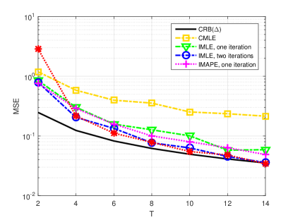
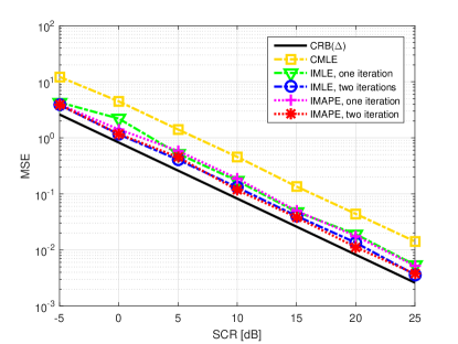
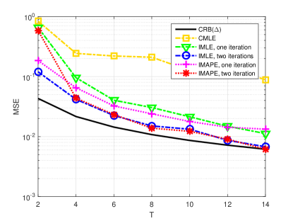
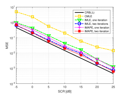
Remark 1: The convergence of the LL function in our algorithm is guaranteed by the fact that the value of the objective function at each step can either improve or maintain but cannot increase[33]. In fact, as the simulations in Section 7 show, the convergence of the estimate of the unknown parameter ΔΔ\Delta can also be observed with only two iteration, a result in accordance with those in [32] and [33]. Here the convergence of ΔΔ\Delta is defined as that Δ^(i+1)Δ^(i)normsuperscript^Δ𝑖1superscript^Δ𝑖\left\|\hat{\Delta}^{(i+1)}-\hat{\Delta}^{(i)}\right\| falls into a small range ϵitalic-ϵ\epsilon, and further iterations do not lead to substantial improvement of performance in terms of the resulting mean square errors (MSEs).

Remark 2: Based on the observation in Remark 1, we can conclude that the computational cost of our algorithm, which lies mainly in the solution of the highly nonlinear optimization problem in Step 2, is only a few times of that of the conventional MLE (CMLE). The latter corresponds to the case where the clutter is assumed to be uniform white Gaussian, such that Eq. (19) degenerate into:

Δ^CMLE=argminΔ{𝚷𝑩(Δ)𝒚}.subscript^ΔCMLEsubscriptΔnormsuperscriptsubscript𝚷𝑩Δbottom𝒚\hat{\Delta}_{\text{CMLE}}=\arg\min_{\Delta}\left\{\left\|\boldsymbol{\Pi}_{{\boldsymbol{B}}(\Delta)}^{\bot}{\boldsymbol{y}}\right\|\right\}. (21)

Remark 3: One should also notice that, in the case where T<N𝑇𝑁T<N, the sample covariance matrix is rank deficient. In this case, the Moore-Penrose pseudoinverse rather than the true inverse should be used for the calculation of 𝚺1superscript𝚺1\boldsymbol{\Sigma}^{-1} in Eqs. (12) and (14), as well as of 𝑮1/2superscript𝑮12\boldsymbol{G}^{-1/2} in the expression of 𝑩ˇ(Δ)ˇ𝑩Δ\check{\boldsymbol{B}}(\Delta) and 𝒚ˇˇ𝒚\check{\boldsymbol{y}}.

4 Iterative Maximum A Posteriori Estimator

The IMLE presented in Section 3, in which we treat the texture as deterministic and thereby ignore information regarding its statistical properties, has the advantage of easier and faster implementation. It is also a natural approach when the texture does not have a closed-form expression of distribution (e.g., in the case of Weibull clutter) or its distribution is unknown. In general cases, however, such approach is suboptimal. In this section, we propose the IMAPE, which is also based on the idea of numerical concentration. Nevertheless, unlike the IMLE, the proposed IMAPE exploits information from the texture’s prior distribution and leads to superior performance.

The maximum a posteriori estimator maximizes the joint LL function, denoted by ΛJsubscriptΛJ\Lambda_{\text{J}}, which is equal to:

ΛJsubscriptΛJ\displaystyle\Lambda_{\text{J}} =lnp𝒚,𝝉(𝒚,𝝉;𝝃)=ln(p𝒚|𝝉(𝒚|𝝉;𝝍)p𝝉(𝝉;a,b))absentsubscript𝑝𝒚𝝉𝒚𝝉𝝃subscript𝑝conditional𝒚𝝉conditional𝒚𝝉𝝍subscript𝑝𝝉𝝉𝑎𝑏\displaystyle=\ln p_{\boldsymbol{y},\boldsymbol{\tau}}\left(\boldsymbol{y},\boldsymbol{\tau};\boldsymbol{\xi}\right)=\ln\left(p_{\boldsymbol{y}|\boldsymbol{\tau}}\left(\boldsymbol{y}|\boldsymbol{\tau};\boldsymbol{\psi}\right)p_{\boldsymbol{\tau}}(\boldsymbol{\tau};a,b)\right) (22)
=ΛC+t=1Tlnpτ(t)(τ(t);a,b)absentsubscriptΛCsuperscriptsubscript𝑡1𝑇subscript𝑝𝜏𝑡𝜏𝑡𝑎𝑏\displaystyle=\Lambda_{\text{C}}+\sum_{t=1}^{T}\ln p_{\tau(t)}(\tau(t);a,b)
={ΛCTlnΓ(a)Talnb+(a1)t=1Tlnτ(t)t=1Tτ(t)b,K-distributed clutter,ΛCTlnΓ(a)+Talnb(a+1)t=1Tlnτ(t)bt=1T1τ(t),t-distributed clutter.\displaystyle=\left\{\begin{aligned} &\Lambda_{\text{C}}-T\ln\Gamma(a)-Ta\ln{b}+(a-1)\sum_{t=1}^{T}\ln\tau(t)\\ &-\frac{\sum_{t=1}^{T}\tau(t)}{b},\quad\text{K-distributed clutter},\\ &\Lambda_{\text{C}}-T\ln\Gamma(a)+Ta\ln{b}-(a+1)\sum_{t=1}^{T}\ln\tau(t)\\ &-b\sum_{t=1}^{T}\frac{1}{\tau(t)},\quad\text{t-distributed clutter}.\end{aligned}\right.

The expression of τ^(t)^𝜏𝑡\hat{\tau}(t), when all the remaining unknown parameters are fixed, can be found by solving ΛJ/τ(t)=0subscriptΛJ𝜏𝑡0\partial\Lambda_{\text{J}}/\partial\tau(t)=0, as:

τ^(t)={12((aN1)b+((aN1)2b2+4b(𝒚(t)𝒗(t))H𝚺1(𝒚(t)𝒗(t)))12),K-distributed clutter,(𝒚(t)𝒗(t))H𝚺1(𝒚(t)𝒗(t))+ba+N+1,t-distributed clutter.\hat{\tau}(t)=\left\{\begin{aligned} &\frac{1}{2}\bigg{(}\left(a-N-1\right)b+\Big{(}\left(a-N-1\right)^{2}b^{2}\\ &+4b\left(\boldsymbol{y}(t)-\boldsymbol{v}(t)\right)^{H}\boldsymbol{\Sigma}^{-1}\left(\boldsymbol{y}(t)-\boldsymbol{v}(t)\right)\Big{)}^{\frac{1}{2}}\bigg{)},\\ &\qquad\qquad\qquad\qquad\qquad\text{K-distributed clutter},\\ &\frac{\left(\boldsymbol{y}(t)-\boldsymbol{v}(t)\right)^{H}\boldsymbol{\Sigma}^{-1}\left(\boldsymbol{y}(t)-\boldsymbol{v}(t)\right)+b}{a+N+1},\\ &\qquad\qquad\qquad\qquad\qquad\text{t-distributed clutter}.\end{aligned}\right. (23)

A comparison between the expressions of τ^(t)^𝜏𝑡\hat{\tau}(t) in Eq. (12) and in Eq. (23) reveals that the latter takes into account the statistical properties of the texture. In these expressions, the parameters a𝑎a and b𝑏b play the roles of scale/translation factors to enhance the estimation of τ(t)𝜏𝑡\tau(t). This is more easily perceptible in the case of a t-distributed clutter, where the expressions for τ^(t)^𝜏𝑡\hat{\tau}(t) in Eq. (12) and (23) have a similar form. For example, the case of large b𝑏b and small a𝑎a corresponds to a more heavily-tailed distribution of the texture. This leads to an increased probability of the realization of τ(t)𝜏𝑡\tau(t) with large values. We note that the estimator in Eq. (23), in contrast to that in Eq. (12), adjusts τ^(t)^𝜏𝑡\hat{\tau}(t) in a way that prevents the occurrence of small values and encourages that of larger ones.

Next, we consider the estimate of the texture parameters a𝑎a and b𝑏b, denoted by a^^𝑎\hat{a} and b^^𝑏\hat{b}. The latter can be obtained by solving ΛJ/b=0subscriptΛJ𝑏0\partial\Lambda_{\text{J}}/\partial b=0, as:

b^={t=1Tτ(t)Ta,K-distributed clutter,Tat=1T1τ(t),t-distributed clutter.\hat{b}=\left\{\begin{aligned} &\frac{\sum_{t=1}^{T}\tau(t)}{Ta},\quad\text{K-distributed clutter},\\ &\frac{Ta}{\sum_{t=1}^{T}\frac{1}{\tau(t)}},\quad\text{t-distributed clutter}.\end{aligned}\right. (24)

On the other hand, calculating ΛJ/asubscriptΛJ𝑎\partial\Lambda_{\text{J}}/\partial a yields:

ΛJa={TΨ(a)Tlnb+t=1Tlnτ(t),K-distributed clutter,TΨ(a)+Tlnbt=1Tlnτ(t),t-distributed clutter,\frac{\partial\Lambda_{\text{J}}}{\partial a}=\left\{\begin{aligned} &-T\Psi(a)-T\ln b+\sum_{t=1}^{T}\ln\tau(t),\quad\text{K-distributed clutter},\\ &-T\Psi(a)+T\ln b-\sum_{t=1}^{T}\ln\tau(t),\quad\text{t-distributed clutter},\end{aligned}\right. (25)

in which Ψ()Ψ\Psi(\cdot) stands for the digamma function. From Eq. (25) it turns out that ΛJ/a=0subscriptΛJ𝑎0\partial\Lambda_{\text{J}}/\partial a=0 does not allow an analytical expression of the root, thus a^^𝑎\hat{a}, unlike b^^𝑏\hat{b} in Eq. (24), can only be calculated numerically. Eqs. (23)-(25) reveal that the estimates of τ(t)𝜏𝑡\tau(t), a𝑎a and b𝑏b are mutually dependent, and further dependent on the parameter vector 𝝍𝝍\boldsymbol{\psi}.

Now, let us approach the estimation of the target parameters and the speckle covariance matrix. The same expressions of 𝚺^^𝚺\hat{\boldsymbol{\Sigma}} and 𝜶^^𝜶\hat{\boldsymbol{\alpha}} in Eqs. (13) and (17), that we obtained for the IMLE, are also valid in the case of the IMAPE, because ΛJ/𝚺=ΛC/𝚺subscriptΛJ𝚺subscriptΛC𝚺\partial\Lambda_{\text{J}}/\partial{\boldsymbol{\Sigma}}=\partial\Lambda_{\text{C}}/\partial{\boldsymbol{\Sigma}} and ΛJ/𝜶=ΛC/𝜶subscriptΛJ𝜶subscriptΛC𝜶\partial\Lambda_{\text{J}}/\partial{\boldsymbol{\alpha}}=\partial\Lambda_{\text{C}}/\partial{\boldsymbol{\alpha}}. Substituting τ^(t)^𝜏𝑡\hat{\tau}(t) in Eq. (23) into Eq. (13), we arrive at the following iterative expression for 𝚺^^𝚺\hat{\boldsymbol{\Sigma}}:

𝚺^(i+1)={2Tt=1T(𝒚(t)𝒗(t))(𝒚(t)𝒗(t))H/((4b(𝒚(t)𝒗(t))H(𝚺^(i))1(𝒚(t)𝒗(t))+(aN1)2b2)12+(aN1)b),K-distributed clutter,a+N+1Tt=1T((𝒚(t)𝒗(t))(𝒚(t)𝒗(t))H)/((𝒚(t)𝒗(t))H(𝚺^(i))1(𝒚(t)𝒗(t))+b),t-distributed clutter,\hat{\boldsymbol{\Sigma}}^{(i+1)}=\left\{\begin{aligned} &\frac{2}{T}\sum_{t=1}^{T}\left(\boldsymbol{y}(t)-\boldsymbol{v}(t)\right)\left(\boldsymbol{y}(t)-\boldsymbol{v}(t)\right)^{H}\\ &\left.\middle/\Bigg{(}\right.\bigg{(}4b\left(\boldsymbol{y}(t)-\boldsymbol{v}(t)\right)^{H}\left(\hat{\boldsymbol{\Sigma}}^{(i)}\right)^{-1}\\ &\cdot\left(\boldsymbol{y}(t)-\boldsymbol{v}(t)\right)+\left(a-N-1\right)^{2}b^{2}\bigg{)}^{\frac{1}{2}}\\ &+\left(a-N-1\right)b\Bigg{)},\quad\text{K-distributed clutter},\\ &\frac{a+N+1}{T}\sum_{t=1}^{T}\Big{(}\left(\boldsymbol{y}(t)-\boldsymbol{v}(t)\right)\\ &\cdot\left(\boldsymbol{y}(t)-\boldsymbol{v}(t)\right)^{H}\Big{)}\\ &\left.\middle/\bigg{(}\right.\left(\boldsymbol{y}(t)-\boldsymbol{v}(t)\right)^{H}\left(\hat{\boldsymbol{\Sigma}}^{(i)}\right)^{-1}\\ &\cdot\left(\boldsymbol{y}(t)-\boldsymbol{v}(t)\right)+b\bigg{)},\quad\text{t-distributed clutter},\end{aligned}\right. (26)

which, similar to the expression of 𝚺^(i+1)superscript^𝚺𝑖1\hat{\boldsymbol{\Sigma}}^{(i+1)} in Eq. (14) for the IMLE, needs to be substituted into Eq. (15) to obtain the normalized 𝚺^(i+1)superscript^𝚺𝑖1\hat{\boldsymbol{\Sigma}}^{(i+1)} denoted as 𝚺^n(i+1)subscriptsuperscript^𝚺𝑖1n\hat{\boldsymbol{\Sigma}}^{(i+1)}_{\text{n}}.

Finally, we address the estimation of ΔΔ\Delta. Adopting the numerical concentration approach similar to that in Section 3, we assume here that 𝚺𝚺\boldsymbol{\Sigma} and 𝝉𝝉\boldsymbol{\tau} to be known from the previous iteration of the algorithm. Furthermore, as the estimates of a𝑎a and b𝑏b are only dependent on 𝝉𝝉\boldsymbol{\tau}, these are also fixed for each iteration. Thus, we may drop in the expression of the joint LL function ΛJsubscriptΛJ\Lambda_{\text{J}} in Eq. (22) those terms that contain only these parameters, transforming it into the same expression as in Eq. (18). This means that ΔΔ\Delta can be obtained, also for the IMAPE, from Eq. (19).

The iterative estimation procedure of the proposed IMAPE also contains three steps and is summarized as follows:

  • Step 1: Initialization. At iteration i=0𝑖0i=0, set τ^(0)(t)=1,t=1,,Tformulae-sequencesuperscript^𝜏0𝑡1𝑡1𝑇\hat{\tau}^{(0)}(t)=1,\ t=1,\dots,T, and 𝚺^n(0)=1/N𝑰Nsubscriptsuperscript^𝚺0n1𝑁subscript𝑰𝑁\hat{\boldsymbol{\Sigma}}^{(0)}_{\text{n}}=1/N\cdot\boldsymbol{I}_{N}.

  • Step 2: Calculate Δ^(i)superscript^Δ𝑖\hat{\Delta}^{(i)} from Eq. (19) using τ^(i)(t)superscript^𝜏𝑖𝑡\hat{\tau}^{(i)}(t) and 𝚺^n(i)subscriptsuperscript^𝚺𝑖n\hat{\boldsymbol{\Sigma}}^{(i)}_{\text{n}}, then 𝜶^(i)superscript^𝜶𝑖\hat{\boldsymbol{\alpha}}^{(i)} from Eq. (17) using Δ^(i)superscript^Δ𝑖\hat{\Delta}^{(i)}, τ^(i)(t)superscript^𝜏𝑖𝑡\hat{\tau}^{(i)}(t) and 𝚺^n(i)subscriptsuperscript^𝚺𝑖n\hat{\boldsymbol{\Sigma}}^{(i)}_{\text{n}}. Next, calculate 𝒗^(i)(t)superscript^𝒗𝑖𝑡\hat{\boldsymbol{v}}^{(i)}(t) from Eq. (16) using Δ^(i)superscript^Δ𝑖\hat{\Delta}^{(i)} and 𝜶^(i)superscript^𝜶𝑖\hat{\boldsymbol{\alpha}}^{(i)}. Finally, substitute Eq. (24) into Eq. (25), and find numerically a^(i)superscript^𝑎𝑖\hat{a}^{(i)} from Eq. (25) using τ^(i)(t)superscript^𝜏𝑖𝑡\hat{\tau}^{(i)}(t), then find b^(i)superscript^𝑏𝑖\hat{b}^{(i)} from Eq. (24) using τ^(i)(t)superscript^𝜏𝑖𝑡\hat{\tau}^{(i)}(t) and a^(i)superscript^𝑎𝑖\hat{a}^{(i)}.

  • Step 3: Use 𝒗^(i)(t)superscript^𝒗𝑖𝑡\hat{\boldsymbol{v}}^{(i)}(t), 𝚺^n(i)subscriptsuperscript^𝚺𝑖n\hat{\boldsymbol{\Sigma}}^{(i)}_{\text{n}}, a^(i)superscript^𝑎𝑖\hat{a}^{(i)} and b^(i)superscript^𝑏𝑖\hat{b}^{(i)} to update 𝚺^n(i+1)subscriptsuperscript^𝚺𝑖1n\hat{\boldsymbol{\Sigma}}^{(i+1)}_{\text{n}} from Eqs. (26) and (15). Then, use 𝒗^(i)(t)superscript^𝒗𝑖𝑡\hat{\boldsymbol{v}}^{(i)}(t), a^(i)superscript^𝑎𝑖\hat{a}^{(i)}, b^(i)superscript^𝑏𝑖\hat{b}^{(i)} and the updated 𝚺^n(i+1)subscriptsuperscript^𝚺𝑖1n\hat{\boldsymbol{\Sigma}}^{(i+1)}_{\text{n}} to find the updated τ^(i+1)(t)superscript^𝜏𝑖1𝑡\hat{\tau}^{(i+1)}(t) from Eq. (23). Set i=i+1𝑖𝑖1i=i+1.

Repeat Step 2 and Step 3 until a stop criterion (convergence or a maximum number of iteration) to obtain the final Δ^^Δ\hat{\Delta}, denoted by Δ^IMAPEsubscript^ΔIMAPE\hat{\Delta}_{\text{IMAPE}}.

Note that Remarks 1-3 of Section 3 also directly apply to the proposed IMAPE.

5 Cramér-Rao-like bounds

The CRLBs provide an essential tool for evaluating the performance of any unbiased estimator. Furthermore, closed-form expressions of the CRLBs are required in the computation of the expression for the ARL in Smith’s sense. In this section, we derive the expressions of various CRLBs w.r.t. ΔΔ\Delta, including the standard CRB, the EMCB, the MCRB and the HCRB, and provides a comparison between them.

5.1 Standard Cramér-Rao Bound

In [34], we have derived the expression for the standard CRB w.r.t. ΔΔ\Delta, denoted by CRB(Δ)CRBΔ\text{CRB}(\Delta), under a K-distributed clutter. This result also holds true for the t-distributed clutter case, except for the factor κ𝜅\kappa (that will be detailed later), which takes another expression under a t-distributed clutter.

CRB(Δ)CRBΔ\text{CRB}(\Delta) considers the parameter vector 𝝃𝝃\boldsymbol{\xi}, and is obtained as the upper-leftmost element of the inverse of the Fisher Information Matrix (FIM), denoted by 𝑭𝑭\boldsymbol{F}. The FIM is calculated from the marginal likelihood p𝒚(𝒚;𝝃)subscript𝑝𝒚𝒚𝝃p_{\boldsymbol{y}}\left(\boldsymbol{y};\boldsymbol{\xi}\right) in Eq. (10). The elements of 𝑭𝑭\boldsymbol{F} are given by:

[𝑭]i,j=E𝒚{ln(p𝒚(𝒚;𝝃))[𝝃]iln(p𝒚(𝒚;𝝃))[𝝃]j},subscriptdelimited-[]𝑭𝑖𝑗subscriptE𝒚subscript𝑝𝒚𝒚𝝃subscriptdelimited-[]𝝃𝑖subscript𝑝𝒚𝒚𝝃subscriptdelimited-[]𝝃𝑗\left[\boldsymbol{F}\right]_{i,j}=\text{E}_{\boldsymbol{y}}\left\{\frac{\partial\ln\left(p_{\boldsymbol{y}}\left(\boldsymbol{y};\boldsymbol{\xi}\right)\right)}{\partial\left[\boldsymbol{\xi}\right]_{i}}\frac{\partial\ln\left(p_{\boldsymbol{y}}\left(\boldsymbol{y};\boldsymbol{\xi}\right)\right)}{\partial\left[\boldsymbol{\xi}\right]_{j}}\right\}, (27)

in which []i,jsubscriptdelimited-[]𝑖𝑗[\cdot]_{i,j} denotes the (i,j)𝑖𝑗(i,j)th entry of a matrix, and []isubscriptdelimited-[]𝑖[\cdot]_{i} denotes the i𝑖ith element of a vector. Derivations show that 𝑭𝑭\boldsymbol{F} takes the following block-diagonal structured form:

𝑭=[𝚽𝟎5×(N2+2)𝟎(N2+2)×5𝚵],𝑭delimited-[]𝚽subscript05superscript𝑁22subscript0superscript𝑁225𝚵\boldsymbol{F}=\left[\begin{array}[]{cc}\boldsymbol{\Phi}&\boldsymbol{0}_{5\times(N^{2}+2)}\\ \boldsymbol{0}_{(N^{2}+2)\times 5}&\boldsymbol{\Xi}\end{array}\right], (28)

in which 𝚽𝚽\boldsymbol{\Phi} denotes the 5×5555\times 5 FIM block w.r.t. the target parameters (those in 𝝁𝝁\boldsymbol{\mu}), whose entries, denoted by ϕijsubscriptitalic-ϕ𝑖𝑗\phi_{ij}, are given by:

ϕij=2κNt=1Ttr{𝒗i(t)𝒗jH(t)𝚺1}¯,i,j=1,,5,formulae-sequencesubscriptitalic-ϕ𝑖𝑗2𝜅𝑁superscriptsubscript𝑡1𝑇¯trsubscript𝒗𝑖𝑡subscriptsuperscript𝒗𝐻𝑗𝑡superscript𝚺1𝑖𝑗15\phi_{ij}=\frac{2\kappa}{N}\sum_{t=1}^{T}\overline{\text{tr}\left\{\boldsymbol{v}_{i}(t)\boldsymbol{v}^{H}_{j}(t)\boldsymbol{\Sigma}^{-1}\right\}},\ i,j=1,\dots,5, (29)

where 𝒗i(t)=𝒗(t)/[𝝁]isubscript𝒗𝑖𝑡𝒗𝑡subscriptdelimited-[]𝝁𝑖\boldsymbol{v}_{i}(t)=\partial\boldsymbol{v}(t)/\partial\left[\boldsymbol{\mu}\right]_{i}. The matrix 𝚵𝚵\boldsymbol{\Xi} in Eq. (28) represents the FIM block w.r.t. the clutter parameters (a𝑎a, b𝑏b and [𝜻]isubscriptdelimited-[]𝜻𝑖\left[\boldsymbol{\zeta}\right]_{i}). As 𝚽𝚽\boldsymbol{\Phi} and 𝚵𝚵\boldsymbol{\Xi} are decoupled, we have:

CRB(Δ)=[𝚽1]1,1.CRBΔsubscriptdelimited-[]superscript𝚽111\text{CRB}\left(\Delta\right)=\left[\boldsymbol{\Phi}^{-1}\right]_{1,1}. (30)

The expression of the positive real factor κ𝜅\kappa in Eq. (29) depends on the distribution of the texture and is given by:

κ={0+xN+a1KaN12(x)KaN(x)dx2N+a2bΓ(N)Γ(a),K-distributed clutter,Na(a+N)b(a+N+1),t-distributed clutter;\kappa=\left\{\begin{aligned} &\frac{\int_{0}^{+\infty}x^{N+a-1}\frac{K_{a-N-1}^{2}(x)}{K_{a-N}(x)}\text{d}x}{2^{N+a-2}b\Gamma(N)\Gamma(a)},\quad\text{K-distributed clutter},\\ &\frac{Na(a+N)}{b(a+N+1)},\quad\text{t-distributed clutter};\end{aligned}\right. (31)

in which Kn(x)subscript𝐾𝑛𝑥K_{n}(x) is the modified Bessel functions of the second kind of order n𝑛n. For a t-distributed clutter, Eq. (31) is a generalization of the result in [26] to the two texture parameter cases. For a K-distributed clutter, we have found a more compact expression of κ𝜅\kappa than [26], which yet still can only be evaluated numerically.

5.2 Extended Miller-Chang Bound

The EMCB was first proposed in [59] as an extension to the conventional Miller-Chang Bound (MCB) [60]. Its general motivation is to first treat the random nuisance parameters (𝝉𝝉\boldsymbol{\tau} in our case) as deterministic and derive the CRB calculated from the conditional likelihood p𝒚|𝝉(𝒚|𝝉;𝝍)subscript𝑝conditional𝒚𝝉conditional𝒚𝝉𝝍p_{\boldsymbol{y}|\boldsymbol{\tau}}\left(\boldsymbol{y}|\boldsymbol{\tau};\boldsymbol{\psi}\right) in Eq. (8). Then in the next step, the assumption of constant 𝝉𝝉\boldsymbol{\tau} is relaxed and the CRB is averaged over different realizations of 𝝉𝝉\boldsymbol{\tau} drawn from the corresponding random distribution. This approach has in common with the proposed IMLE in Section 3, that the latter also treats 𝝉𝝉\boldsymbol{\tau} to be deterministic. The performance of this algorithm, in terms of the averaged MSE resulting from many independent Monte-Carlo trials, can be evaluated by averaging the CRBs calculated for each of the trials. It is clear that such an averaged CRB, when the trial number becomes large, approaches the EMCB.

The parameter vector [𝝍T,𝝉T]Tsuperscriptsuperscript𝝍𝑇superscript𝝉𝑇𝑇[\boldsymbol{\psi}^{T},\boldsymbol{\tau}^{T}]^{T} is considered in the calculation of the EMCB. The entries of the corresponding FIM, denoted by 𝑭Esubscript𝑭E\boldsymbol{F}_{\text{E}}, are calculated by:

[𝑭E]i,j=E𝒚|𝝉{ln(p𝒚|𝝉(𝒚|𝝉;𝝍))[𝝍]iln(p𝒚|𝝉(𝒚,|𝝉;𝝍))[𝝍]j}.\left[\boldsymbol{F}_{\text{E}}\right]_{i,j}=\text{E}_{\boldsymbol{y}|\boldsymbol{\tau}}\left\{\frac{\partial\ln\left(p_{\boldsymbol{y}|\boldsymbol{\tau}}\left(\boldsymbol{y}|\boldsymbol{\tau};\boldsymbol{\psi}\right)\right)}{\partial\left[\boldsymbol{\psi}\right]_{i}}\frac{\partial\ln\left(p_{\boldsymbol{y}|\boldsymbol{\tau}}\left(\boldsymbol{y},|\boldsymbol{\tau};\boldsymbol{\psi}\right)\right)}{\partial\left[\boldsymbol{\psi}\right]_{j}}\right\}. (32)

whose calculation resembles that of the FIM under Gaussian clutter (with the difference that the data are weighted by 1/τ(t)1𝜏𝑡1/\tau(t) varying at each snapshot) and is omitted here for brevity. Similar to 𝑭𝑭\boldsymbol{F}, 𝑭Esubscript𝑭E\boldsymbol{F}_{\text{E}} exhibits a block-diagonal structure, where the blocks for the target and clutter parameters are decoupled from each other. We denote the parameter block of interest by 𝚽Esubscript𝚽E\boldsymbol{\Phi}_{\text{E}}, and its entries by ϕijE,i,j=1,,5formulae-sequencesubscriptsuperscriptitalic-ϕE𝑖𝑗𝑖𝑗15\phi^{\text{E}}_{ij},\ i,j=1,\dots,5. The following expressions are obtained:

ϕijE=2t=1T1τ(t)tr{𝒗i(t)𝒗jH(t)𝚺1}¯.subscriptsuperscriptitalic-ϕE𝑖𝑗2superscriptsubscript𝑡1𝑇1𝜏𝑡¯trsubscript𝒗𝑖𝑡subscriptsuperscript𝒗𝐻𝑗𝑡superscript𝚺1\phi^{\text{E}}_{ij}=2\sum_{t=1}^{T}\frac{1}{\tau(t)}\overline{\text{tr}\left\{\boldsymbol{v}_{i}(t)\boldsymbol{v}^{H}_{j}(t)\boldsymbol{\Sigma}^{-1}\right\}}. (33)

Consequently, the EMCB w.r.t. ΔΔ\Delta , denoted by EMCB(Δ)EMCBΔ\text{EMCB}\left(\Delta\right), is given by:

EMCB(Δ)=E𝝉{[𝚽E1]1,1},EMCBΔsubscriptE𝝉subscriptdelimited-[]superscriptsubscript𝚽E111\text{EMCB}\left(\Delta\right)=\text{E}_{\boldsymbol{\tau}}\left\{\left[\boldsymbol{\Phi}_{\text{E}}^{-1}\right]_{1,1}\right\}, (34)

for which no closed-form expression exists.

5.3 Modified and Hybrid Cramér-Rao Bound

The MCRB [61], like the EMCB, also considers the unknown parameter vector as [𝝍T,𝝉T]Tsuperscriptsuperscript𝝍𝑇superscript𝝉𝑇𝑇[\boldsymbol{\psi}^{T},\boldsymbol{\tau}^{T}]^{T}. Its corresponding FIM, denoted by 𝑭Msubscript𝑭M\boldsymbol{F}_{\text{M}}, is likewise calculated from the conditional likelihood in Eq. (8). The MCRB differs from the EMCB only in that it averages over the random parameters before the FIM inversion, namely:

[𝑭M]i,j=E𝒚,𝝉{ln(p𝒚|𝝉(𝒚|𝝉;𝝍))[𝝍]iln(p𝒚|𝝉(𝒚,|𝝉;𝝍))[𝝍]j}\displaystyle\left[\boldsymbol{F}_{\text{M}}\right]_{i,j}=\text{E}_{\boldsymbol{y},\boldsymbol{\tau}}\left\{\frac{\partial\ln\left(p_{\boldsymbol{y}|\boldsymbol{\tau}}\left(\boldsymbol{y}|\boldsymbol{\tau};\boldsymbol{\psi}\right)\right)}{\partial\left[\boldsymbol{\psi}\right]_{i}}\frac{\partial\ln\left(p_{\boldsymbol{y}|\boldsymbol{\tau}}\left(\boldsymbol{y},|\boldsymbol{\tau};\boldsymbol{\psi}\right)\right)}{\partial\left[\boldsymbol{\psi}\right]_{j}}\right\} (35)
=E𝝉{E𝒚|𝝉{ln(p𝒚|𝝉(𝒚|𝝉;𝝍))[𝝍]iln(p𝒚|𝝉(𝒚,|𝝉;𝝍))[𝝍]j}}\displaystyle=\text{E}_{\boldsymbol{\tau}}\left\{\text{E}_{\boldsymbol{y}|\boldsymbol{\tau}}\left\{\frac{\partial\ln\left(p_{\boldsymbol{y}|\boldsymbol{\tau}}\left(\boldsymbol{y}|\boldsymbol{\tau};\boldsymbol{\psi}\right)\right)}{\partial\left[\boldsymbol{\psi}\right]_{i}}\frac{\partial\ln\left(p_{\boldsymbol{y}|\boldsymbol{\tau}}\left(\boldsymbol{y},|\boldsymbol{\tau};\boldsymbol{\psi}\right)\right)}{\partial\left[\boldsymbol{\psi}\right]_{j}}\right\}\right\}
=E𝝉{[𝑭E]i,j}.absentsubscriptE𝝉subscriptdelimited-[]subscript𝑭E𝑖𝑗\displaystyle=\text{E}_{\boldsymbol{\tau}}\left\{\left[\boldsymbol{F}_{\text{E}}\right]_{i,j}\right\}.

Similar to 𝑭𝑭\boldsymbol{F} and 𝑭Esubscript𝑭E\boldsymbol{F}_{\text{E}}, 𝑭Msubscript𝑭M\boldsymbol{F}_{\text{M}} also has a block-diagonal structure, whose parameter block of interest, denoted by 𝚽Msubscript𝚽M\boldsymbol{\Phi}_{\text{M}}, contains the following entries ϕijM,i,j=1,,5formulae-sequencesubscriptsuperscriptitalic-ϕM𝑖𝑗𝑖𝑗15\phi^{\text{M}}_{ij},\ i,j=1,\dots,5:

ϕijM=E𝝉{[𝚽E1]i,j}=2νt=1Ttr{𝒗i(t)𝒗jH(t)𝚺1}¯,subscriptsuperscriptitalic-ϕM𝑖𝑗subscriptE𝝉subscriptdelimited-[]superscriptsubscript𝚽E1𝑖𝑗2𝜈superscriptsubscript𝑡1𝑇¯trsubscript𝒗𝑖𝑡subscriptsuperscript𝒗𝐻𝑗𝑡superscript𝚺1\phi^{\text{M}}_{ij}=\text{E}_{\boldsymbol{\tau}}\left\{\left[\boldsymbol{\Phi}_{\text{E}}^{-1}\right]_{i,j}\right\}=2\nu\sum_{t=1}^{T}\overline{\text{tr}\left\{\boldsymbol{v}_{i}(t)\boldsymbol{v}^{H}_{j}(t)\boldsymbol{\Sigma}^{-1}\right\}}, (36)

in which

ν=E{1τ(t)}={2b(a1),K-distributed clutter, for a>1,2ab,t-distributed clutter,\nu=\text{E}\left\{\frac{1}{\tau(t)}\right\}=\left\{\begin{aligned} &\frac{2}{b(a-1)},\quad\text{K-distributed clutter, for $a>1$},\\ &\frac{2a}{b},\quad\text{t-distributed clutter},\end{aligned}\right. (37)

and the MCRB w.r.t. ΔΔ\Delta, denoted by MCRB(Δ)MCRBΔ\text{MCRB}\left(\Delta\right), is equal to:

MCRB(Δ)=[𝚽M1]1,1.MCRBΔsubscriptdelimited-[]superscriptsubscript𝚽M111\text{MCRB}\left(\Delta\right)=\left[\boldsymbol{\Phi}_{\text{M}}^{-1}\right]_{1,1}. (38)

The HCRB as defined in [62], on the other hand, considers the unknown parameter vector as [𝝃T,𝝉T]Tsuperscriptsuperscript𝝃𝑇superscript𝝉𝑇𝑇[\boldsymbol{\xi}^{T},\boldsymbol{\tau}^{T}]^{T}. Furthermore, it uses the joint likelihood in Eq. (9), instead of the conditional likelihood in Eq. (8), similar as in the derivation of the EMCB and MCRB, to obtain its FIM, which is denoted by 𝑭Hsubscript𝑭H\boldsymbol{F}_{\text{H}}. The entries of 𝑭Hsubscript𝑭H\boldsymbol{F}_{\text{H}} are calculated by:

ϕijH=E𝒚,𝝉{ln(p𝒚,𝝉(𝒚,𝝉;𝝃))[𝝃]iln(p𝒚,𝝉(𝒚,𝝉;𝝃))[𝝃]j}.subscriptsuperscriptitalic-ϕH𝑖𝑗subscriptE𝒚𝝉subscript𝑝𝒚𝝉𝒚𝝉𝝃subscriptdelimited-[]𝝃𝑖subscript𝑝𝒚𝝉𝒚𝝉𝝃subscriptdelimited-[]𝝃𝑗\phi^{\text{H}}_{ij}=\text{E}_{\boldsymbol{y},\boldsymbol{\tau}}\left\{\frac{\partial\ln\left(p_{\boldsymbol{y},\boldsymbol{\tau}}\left(\boldsymbol{y},\boldsymbol{\tau};\boldsymbol{\xi}\right)\right)}{\partial\left[\boldsymbol{\xi}\right]_{i}}\frac{\partial\ln\left(p_{\boldsymbol{y},\boldsymbol{\tau}}\left(\boldsymbol{y},\boldsymbol{\tau};\boldsymbol{\xi}\right)\right)}{\partial\left[\boldsymbol{\xi}\right]_{j}}\right\}. (39)

Our derivations show that 𝑭Hsubscript𝑭H\boldsymbol{F}_{\text{H}} also has a block structure, and its parameter block of interest is equal to that of the MCRB, 𝚽Msubscript𝚽M\boldsymbol{\Phi}_{\text{M}}. Consequently, we have:

HCRB(Δ)=MCRB(Δ),HCRBΔMCRBΔ\text{HCRB}\left(\Delta\right)=\text{MCRB}\left(\Delta\right), (40)

in which HCRB(Δ)HCRBΔ\text{HCRB}\left(\Delta\right) represents the HCRB w.r.t. ΔΔ\Delta.

5.4 Relationships between the CRLBs

It is theoretically proved in [62] that the standard CRB is always larger than the HCRB. As we also have HCRB(Δ)=MCRB(Δ)HCRBΔMCRBΔ\text{HCRB}\left(\Delta\right)=\text{MCRB}\left(\Delta\right), it follows that:

CRB(Δ)HCRB(Δ)=MCRB(Δ).CRBΔHCRBΔMCRBΔ\text{CRB}\left(\Delta\right)\geq\text{HCRB}\left(\Delta\right)=\text{MCRB}\left(\Delta\right). (41)

This relationship, however, becomes apparent when the clutter follows a t-distribution, where CRB(Δ)CRBΔ\text{CRB}\left(\Delta\right) has a closed-form expression. By comparison of Eqs. (29)-(31) with Eqs. (30), (36) and (40), we have:

CRB(Δ)MCRB(Δ)=CRB(Δ)HCRB(Δ)=a+N+1a+N>1.CRBΔMCRBΔCRBΔHCRBΔ𝑎𝑁1𝑎𝑁1\frac{\text{CRB}\left(\Delta\right)}{\text{MCRB}\left(\Delta\right)}=\frac{\text{CRB}\left(\Delta\right)}{\text{HCRB}\left(\Delta\right)}=\frac{a+N+1}{a+N}>1. (42)

Moreover, since (a+N+1)/(a+N)1𝑎𝑁1𝑎𝑁1(a+N+1)/(a+N)\rightarrow 1 when N𝑁N\rightarrow\infty, it follows that CRB(Δ)MCRB(Δ)=HCRB(Δ)CRBΔMCRBΔHCRBΔ\text{CRB}(\Delta)\rightarrow\text{MCRB}(\Delta)=\text{HCRB}(\Delta) when the number of receiver antennas becomes large.

The relationship between EMCB(Δ)EMCBΔ\text{EMCB}(\Delta) and MCRB(Δ)MCRBΔ\text{MCRB}\left(\Delta\right) (or HCRB(Δ)HCRBΔ\text{HCRB}\left(\Delta\right)) can be revealed by noticing, from Eq. (34), that:

EMCB(Δ)=E𝝉{[𝚽E1]1,1}=[E𝝉{𝚽E1}]1,1,EMCBΔsubscriptE𝝉subscriptdelimited-[]superscriptsubscript𝚽E111subscriptdelimited-[]subscriptE𝝉superscriptsubscript𝚽E111\text{EMCB}(\Delta)=\text{E}_{\boldsymbol{\tau}}\left\{\left[\boldsymbol{\Phi}_{\text{E}}^{-1}\right]_{1,1}\right\}=\left[\text{E}_{\boldsymbol{\tau}}\left\{\boldsymbol{\Phi}_{\text{E}}^{-1}\right\}\right]_{1,1}, (43)

and, according to Eqs. (35) and (38), that:

MCRB(Δ)=[𝚽M1]1,1=[(E𝝉{𝚽E})1]1,1.MCRBΔsubscriptdelimited-[]superscriptsubscript𝚽M111subscriptdelimited-[]superscriptsubscriptE𝝉subscript𝚽E111\text{MCRB}(\Delta)=\left[\boldsymbol{\Phi}_{\text{M}}^{-1}\right]_{1,1}=\left[\left(\text{E}_{\boldsymbol{\tau}}\left\{\boldsymbol{\Phi}_{\text{E}}\right\}\right)^{-1}\right]_{1,1}. (44)

Since 𝚽E1superscriptsubscript𝚽E1\boldsymbol{\Phi}_{\text{E}}^{-1} is a convex function of the entries of 𝚽Esubscript𝚽E\boldsymbol{\Phi}_{\text{E}} [63], by Jensen’s inequality, we have:

E𝝉{𝚽E1}(E𝝉{𝚽E})1𝟎,succeeds-or-equalssubscriptE𝝉superscriptsubscript𝚽E1superscriptsubscriptE𝝉subscript𝚽E10\text{E}_{\boldsymbol{\tau}}\left\{\boldsymbol{\Phi}_{\text{E}}^{-1}\right\}-\left(\text{E}_{\boldsymbol{\tau}}\left\{\boldsymbol{\Phi}_{\text{E}}\right\}\right)^{-1}\succeq\boldsymbol{0}, (45)

Hence [E𝝉{𝚽E1}]1,1[(E𝝉{𝚽E})1]1,1subscriptdelimited-[]subscriptE𝝉superscriptsubscript𝚽E111subscriptdelimited-[]superscriptsubscriptE𝝉subscript𝚽E111\left[\text{E}_{\boldsymbol{\tau}}\left\{\boldsymbol{\Phi}_{\text{E}}^{-1}\right\}\right]_{1,1}\geq\left[\left(\text{E}_{\boldsymbol{\tau}}\left\{\boldsymbol{\Phi}_{\text{E}}\right\}\right)^{-1}\right]_{1,1}, viz.,

EMCB(Δ)MCRB(Δ)=HCRB(Δ).EMCBΔMCRBΔHCRBΔ\text{EMCB}(\Delta)\geq\text{MCRB}(\Delta)=\text{HCRB}(\Delta). (46)

Furthermore, since 𝚽E𝚽Msubscript𝚽Esubscript𝚽M\boldsymbol{\Phi}_{\text{E}}\rightarrow\boldsymbol{\Phi}_{\text{M}} when T𝑇T\rightarrow\infty, we have that EMCB(Δ)MCRB(Δ)=HCRB(Δ)EMCBΔMCRBΔHCRBΔ\text{EMCB}(\Delta)\rightarrow\text{MCRB}(\Delta)=\text{HCRB}(\Delta) as the number of snapshots becomes large.

The relationship between CRB(Δ)CRBΔ\text{CRB}(\Delta) and EMCB(Δ)EMCBΔ\text{EMCB}(\Delta), on the other hand, is indefinite and dependent on T𝑇T and N𝑁N, as will be illustrated by numerical simulations.

5.5 CRLBs and the Texture Parameters

At the end of this section, we investigate the impact of the clutter’s texture parameters, a𝑎a and b𝑏b, on the CRLBs. To achieve this, we first define the signal-to-clutter ratio (SCR) as [26]:

SCR=t=1T𝒔(t)2TE{τ(t)}σ2tr{𝚺ˇ},SCRsuperscriptsubscript𝑡1𝑇superscriptnorm𝒔𝑡2𝑇E𝜏𝑡superscript𝜎2trˇ𝚺\text{SCR}=\frac{\sum_{t=1}^{T}\left\|\boldsymbol{s}(t)\right\|^{2}}{T\text{E}\{\tau(t)\}\sigma^{2}\text{tr}\left\{\check{\boldsymbol{\Sigma}}\right\}}, (47)

in which E{τ(t)}E𝜏𝑡\text{E}\{\tau(t)\} is equal to ab𝑎𝑏ab for a K-distributed clutter and b/(a1)𝑏𝑎1b/(a-1) for a t-distributed clutter (for a>1𝑎1a>1) [64]. It then turns out that for a fixed SCR, we have:

1σ2{a,K-distributed clutter,1a1,t-distributed clutter, for a>1,\frac{1}{\sigma^{2}}\propto\left\{\begin{aligned} &a,\quad\text{K-distributed clutter},\\ &\frac{1}{a-1},\quad\text{t-distributed clutter, for $a>1$},\end{aligned}\right. (48)

and

1σ2b,K-distributed and t-distributed clutters,proportional-to1superscript𝜎2𝑏K-distributed and t-distributed clutters\frac{1}{\sigma^{2}}\propto b,\quad\text{K-distributed and t-distributed clutters}, (49)

in which proportional-to\propto denotes direct proportionality. Furthermore, from Eq. (31), we have:

κ{0+xN+a1KaN12(x)KaN(x)dx2N+a2Γ(a),K-distributed clutter,a(a+N)(a+N+1),t-distributed clutter, for a>1,\kappa\propto\left\{\begin{aligned} &\frac{\int_{0}^{+\infty}x^{N+a-1}\frac{K_{a-N-1}^{2}(x)}{K_{a-N}(x)}\text{d}x}{2^{N+a-2}\Gamma(a)},\quad\text{K-distributed clutter},\\ &\frac{a(a+N)}{(a+N+1)},\quad\text{t-distributed clutter, for $a>1$},\end{aligned}\right. (50)

and

κ1b,K-distributed and t-distributed clutters.proportional-to𝜅1𝑏K-distributed and t-distributed clutters\kappa\propto\frac{1}{b},\quad\text{K-distributed and t-distributed clutters}. (51)

5.5.1 CRLBs vs. a𝑎a

We begin with the standard CRB. The expression in Eq. (29) can be converted to:

ϕij=2κNσ2t=1Ttr{𝒗i(t)𝒗jH(t)𝚺ˇ1}¯,i,j=1,,5,formulae-sequencesubscriptitalic-ϕ𝑖𝑗2𝜅𝑁superscript𝜎2superscriptsubscript𝑡1𝑇¯trsubscript𝒗𝑖𝑡subscriptsuperscript𝒗𝐻𝑗𝑡superscriptˇ𝚺1𝑖𝑗15\phi_{ij}=\frac{2\kappa}{N\sigma^{2}}\sum_{t=1}^{T}\overline{\text{tr}\left\{\boldsymbol{v}_{i}(t)\boldsymbol{v}^{H}_{j}(t)\check{\boldsymbol{\Sigma}}^{-1}\right\}},\ i,j=1,\dots,5, (52)

namely, ϕijκ/σ2proportional-tosubscriptitalic-ϕ𝑖𝑗𝜅superscript𝜎2\phi_{ij}\propto\kappa/\sigma^{2}, to which we apply Eqs. (50) and (48) and have straightforwardly:

ϕij{a0+xN+a1KaN12(x)KaN(x)dx2N+a2Γ(a),K-distributed clutter,a(a+N)(a+N+1)(a1),t-distributed clutter, for a>1.\phi_{ij}\propto\left\{\begin{aligned} &\frac{a\int_{0}^{+\infty}x^{N+a-1}\frac{K_{a-N-1}^{2}(x)}{K_{a-N}(x)}\text{d}x}{2^{N+a-2}\Gamma(a)},\quad\text{K-distributed clutter},\\ &\frac{a(a+N)}{(a+N+1)(a-1)},\quad\text{t-distributed clutter, for $a>1$}.\end{aligned}\right. (53)

For both clutter distributions ϕijsubscriptitalic-ϕ𝑖𝑗\phi_{ij} decreases as a𝑎a increases666This relationship is obvious for t-distributed clutter, for K-distributed clutter, however, for which ϕijsubscriptitalic-ϕ𝑖𝑗\phi_{ij} does not enjoy a closed-form expression, can only be determined numerically.; as a result, CRB(Δ)CRBΔ\text{CRB}\left(\Delta\right) increases with a𝑎a, i.e., the standard CRB is positively correlated with the shape parameter a𝑎a.

Similarly, we deduce from Eqs. (37) and (48) that:

ϕijM=ϕijHaa1,K-distributed and t-distributed clutters,formulae-sequencesubscriptsuperscriptitalic-ϕM𝑖𝑗subscriptsuperscriptitalic-ϕH𝑖𝑗proportional-to𝑎𝑎1K-distributed and t-distributed clutters\phi^{\text{M}}_{ij}=\phi^{\text{H}}_{ij}\propto\frac{a}{a-1},\quad\text{K-distributed and t-distributed clutters}, (54)

also indicating a positive correlation between the MCRB/HCRB and a𝑎a. Furthermore, we notice, as opposed to the standard CRB, which has different proportionalities to a𝑎a for K-distributed and t-distributed clutters respectively, the MCRB/HCRB have the same proportionality for both clutter distributions.

Finally, for the EMCB, we have from Eq. (55) that:

ϕijE=2σ2t=1T1τ(t)tr{𝒗i(t)𝒗jH(t)𝚺ˇ1}¯1σ2t=1T1τ(t).subscriptsuperscriptitalic-ϕE𝑖𝑗2superscript𝜎2superscriptsubscript𝑡1𝑇1𝜏𝑡¯trsubscript𝒗𝑖𝑡subscriptsuperscript𝒗𝐻𝑗𝑡superscriptˇ𝚺1proportional-to1superscript𝜎2superscriptsubscript𝑡1𝑇1𝜏𝑡\phi^{\text{E}}_{ij}=\frac{2}{\sigma^{2}}\sum_{t=1}^{T}\frac{1}{\tau(t)}\overline{\text{tr}\left\{\boldsymbol{v}_{i}(t)\boldsymbol{v}^{H}_{j}(t)\check{\boldsymbol{\Sigma}}^{-1}\right\}}\propto\frac{1}{\sigma^{2}}\sum_{t=1}^{T}\frac{1}{\tau(t)}. (55)

Consequently, it follows from Eq. (34) that:

EMCB(Δ)=σ2E𝝉{1t=1T1τ(t)}.EMCBΔsuperscript𝜎2subscriptE𝝉1superscriptsubscript𝑡1𝑇1𝜏𝑡\text{EMCB}\left(\Delta\right)=\sigma^{2}\text{E}_{\boldsymbol{\tau}}\left\{\frac{1}{\sum_{t=1}^{T}\frac{1}{\tau(t)}}\right\}. (56)

For a t-distributed clutter, τ(t)Inv-Gamma(a,b)similar-to𝜏𝑡Inv-Gamma𝑎𝑏\tau(t)\sim\text{Inv-Gamma}(a,b), 1/τ(t)Gamma(a,1/b)similar-to1𝜏𝑡Gamma𝑎1𝑏1/\tau(t)\sim\text{Gamma}(a,1/b). Thus, as τ(t),t=1,,Tformulae-sequence𝜏𝑡𝑡1𝑇\tau(t),\ t=1,\dots,T are i.i.d. variables, from the property of the gamma distribution arises that 1/t=1T(1/τ(t))Gamma(Ta,1/b)similar-to1superscriptsubscript𝑡1𝑇1𝜏𝑡Gamma𝑇𝑎1𝑏1/\sum_{t=1}^{T}\left(1/\tau(t)\right)\sim\text{Gamma}(Ta,1/b), and consequently,

E𝝉{1t=1T1τ(t)}=Tab,t-distributed clutter,subscriptE𝝉1superscriptsubscript𝑡1𝑇1𝜏𝑡𝑇𝑎𝑏t-distributed clutter\text{E}_{\boldsymbol{\tau}}\left\{\frac{1}{\sum_{t=1}^{T}\frac{1}{\tau(t)}}\right\}=\frac{Ta}{b},\quad\text{t-distributed clutter}, (57)

which, combined with Eqs. (48) and (56), results in EMCB(Δ)a(a1)proportional-toEMCBΔ𝑎𝑎1\text{EMCB}\left(\Delta\right)\propto a(a-1), indicating a positive correlation also between the EMCB and a𝑎a. For a K-distributed clutter an analogous deduction seems, however, impossible or at least complicated, due to the presence of the sum of inverse gamma variables. The relationship between the EMCB and a𝑎a for this case can be numerically ascertained.

5.5.2 CRLBs vs. b𝑏b

Associating Eq. (51) with Eq. (52), yields:

ϕij1bσ2,K-distributed and t-distributed clutters.proportional-tosubscriptitalic-ϕ𝑖𝑗1𝑏superscript𝜎2K-distributed and t-distributed clutters\phi_{ij}\propto\frac{1}{b\sigma^{2}},\quad\text{K-distributed and t-distributed clutters}. (58)

As from Eq. (49) for both clutter distributions b1/σ2proportional-to𝑏1superscript𝜎2b\propto 1/\sigma^{2}, ϕijsubscriptitalic-ϕ𝑖𝑗\phi_{ij} is thus independent of b𝑏b, which means under a fixed SCR, changing b𝑏b does not give rise to any variation in the value of CRB(Δ)CRBΔ\text{CRB}(\Delta). The same also holds true for the MCRB/HCRB for both clutter distributions, and can be established in a similar vein by considering ν𝜈\nu instead of κ𝜅\kappa.

The independence of the EMCB of b𝑏b under t-distributed clutter is straightforwardly confirmable by combining Eqs. (49), (56) and (57). However, under K-distributed clutter, the relationship between the EMCB and b𝑏b can only be determined numerically.

In summary, the performance of the estimation, in terms of the lowest achievable CRLBs, is only related to the shape parameter a𝑎a of the clutter, and decreases as a𝑎a becomes larger, and is independent of the scale paramter b𝑏b. This will also be verified in Section 7 by numerical simulations.

6 Derivation of the ARL

In this section, we address the question of the target resolvability. In order to obtain an analytical expression for the ARL in Smith’s sense, a closed-form (non-matrix) expression for CRB(Δ)CRBΔ\text{CRB}(\Delta) is required. Our above derived CRB(Δ)CRBΔ\text{CRB}(\Delta) in Eq. (30), however, cannot be analytically inverted, due to the nonlinearity of our model in Eq. (1) w.r.t. ΔΔ\Delta. To cope with this difficulty, we first linearize the model [8, 9, 10, 65, 66], and rederive the FIM expression based on it which is feasible for analytical inversion. The ARL obtained from the linearized model approximates the exact ARL obtained from the original model.

6.1 Model Linearization

To linearize the model, we resort to the second order Taylor expansion around Δ=0Δ0\Delta=0 in Eq. (1). This step of approximation is justified by considering the fact that, in asymptotic cases, e.g., those of large SCR or sample size, in which the CRB is a tight bound, the ARL is always very small, i.e., the value of ΔΔ\Delta corresponding to the ARL approaches zero (Δ1much-less-thanΔ1\Delta\ll 1) [39, 40, 66, 36, 67]777This is also supported by the fact that the ML estimator, and generally all high resolution estimators, have asymptotically an infinite resolution capability, leading to the ARL infinitely approaching to 00 [68, 49].. The second order Taylor expansions of 𝒂𝒯(ω2)subscript𝒂𝒯subscript𝜔2\boldsymbol{a}_{\mathcal{T}}\left(\omega_{2}\right) and 𝒂(ω2)subscript𝒂subscript𝜔2\boldsymbol{a}_{\mathcal{R}}\left(\omega_{2}\right) are respectively given by:

𝒂𝒯(ω2)𝒂𝒯(ω1)+jΔ𝒂˙𝒯(ω1)Δ22𝒂¨𝒯(ω1),subscript𝒂𝒯subscript𝜔2subscript𝒂𝒯subscript𝜔1𝑗Δsubscriptbold-˙𝒂𝒯subscript𝜔1superscriptΔ22subscriptbold-¨𝒂𝒯subscript𝜔1\displaystyle\boldsymbol{a}_{\mathcal{T}}\left(\omega_{2}\right)\approx\boldsymbol{a}_{\mathcal{T}}\left(\omega_{1}\right)+j\Delta\boldsymbol{\dot{a}}_{\mathcal{T}}\left(\omega_{1}\right)-\frac{\Delta^{2}}{2}\boldsymbol{\ddot{a}}_{\mathcal{T}}\left(\omega_{1}\right), (59a)
𝒂(ω2)𝒂(ω1)+jΔ𝒂˙(ω1)Δ22𝒂¨(ω1),subscript𝒂subscript𝜔2subscript𝒂subscript𝜔1𝑗Δsubscriptbold-˙𝒂subscript𝜔1superscriptΔ22subscriptbold-¨𝒂subscript𝜔1\displaystyle\boldsymbol{a}_{\mathcal{R}}\left(\omega_{2}\right)\approx\boldsymbol{a}_{\mathcal{R}}\left(\omega_{1}\right)+j\Delta\boldsymbol{\dot{a}}_{\mathcal{R}}\left(\omega_{1}\right)-\frac{\Delta^{2}}{2}\boldsymbol{\ddot{a}}_{\mathcal{R}}\left(\omega_{1}\right), (59b)

where 𝒂˙𝒯()=𝒂𝒯()𝒅𝒯subscriptbold-˙𝒂𝒯direct-productsubscript𝒂𝒯subscript𝒅𝒯\boldsymbol{\dot{a}}_{\mathcal{T}}\left(\cdot\right)=\boldsymbol{a}_{\mathcal{T}}\left(\cdot\right)\odot\boldsymbol{d}_{\mathcal{T}}, 𝒂˙()=𝒂()𝒅subscriptbold-˙𝒂direct-productsubscript𝒂subscript𝒅\boldsymbol{\dot{a}}_{\mathcal{R}}\left(\cdot\right)=\boldsymbol{a}_{\mathcal{R}}\left(\cdot\right)\odot\boldsymbol{d}_{\mathcal{R}}, 𝒂¨𝒯()𝒂𝒯()𝒅𝒯𝒅𝒯subscriptbold-¨𝒂𝒯direct-productsubscript𝒂𝒯subscript𝒅𝒯subscript𝒅𝒯\boldsymbol{\ddot{a}}_{\mathcal{T}}\left(\cdot\right)\triangleq\boldsymbol{a}_{\mathcal{T}}\left(\cdot\right)\odot\boldsymbol{d}_{\mathcal{T}}\odot\boldsymbol{d}_{\mathcal{T}}, 𝒂¨()𝒂()𝒅𝒅subscriptbold-¨𝒂direct-productsubscript𝒂subscript𝒅subscript𝒅\boldsymbol{\ddot{a}}_{\mathcal{R}}\left(\cdot\right)\triangleq\boldsymbol{a}_{\mathcal{R}}\left(\cdot\right)\odot\boldsymbol{d}_{\mathcal{R}}\odot\boldsymbol{d}_{\mathcal{R}}, in which direct-product\odot denotes the Hadamard product, and 𝒅𝒯=[0,d𝒯,,(M1)d𝒯]Tsubscript𝒅𝒯superscript0subscript𝑑𝒯𝑀1subscript𝑑𝒯𝑇\boldsymbol{d}_{\mathcal{T}}=[0,d_{\mathcal{T}},\dots,(M-1)d_{\mathcal{T}}]^{T}, 𝒅=[0,d,,(N1)d]Tsubscript𝒅superscript0subscript𝑑𝑁1subscript𝑑𝑇\boldsymbol{d}_{\mathcal{R}}=[0,d_{\mathcal{R}},\dots,(N-1)d_{\mathcal{R}}]^{T}. One can then approximate Eq. (1) as (omitting all terms containing Δn,n>2superscriptΔ𝑛𝑛2\Delta^{n},\ n>2):

𝒚(t)𝑪(t)𝜼+𝒏(t),t=1,,T;formulae-sequence𝒚𝑡𝑪𝑡𝜼𝒏𝑡𝑡1𝑇\boldsymbol{y}(t)\approx\boldsymbol{C}(t)\boldsymbol{\eta}+\boldsymbol{n}(t),\quad t=1,\dots,T; (60)

where 𝜼=[α1+α2jα2Δα2Δ2]T𝜼superscriptsubscript𝛼1subscript𝛼2𝑗subscript𝛼2Δsubscript𝛼2superscriptΔ2𝑇\boldsymbol{\eta}=\left[\alpha_{1}+\alpha_{2}\quad j\alpha_{2}\Delta\quad-\alpha_{2}\Delta^{2}\right]^{T}, 𝑪(t)=[𝝆1(t)𝝆2(t)𝝆3(t)]𝑪𝑡subscript𝝆1𝑡subscript𝝆2𝑡subscript𝝆3𝑡\boldsymbol{C}(t)=\left[\boldsymbol{\rho}_{1}(t)\quad\boldsymbol{\rho}_{2}(t)\quad\boldsymbol{\rho}_{3}(t)\right], in which 𝝆i(t)=𝑹i𝒔(t),i,j=1,2,3formulae-sequencesubscript𝝆𝑖𝑡subscript𝑹𝑖𝒔𝑡𝑖𝑗123\boldsymbol{\rho}_{i}(t)=\boldsymbol{R}_{i}\boldsymbol{s}(t),\ i,j=1,2,3, where

𝑹1subscript𝑹1\displaystyle\boldsymbol{R}_{1} =\displaystyle= 𝒂(ω1)𝒂𝒯T(ω1),subscript𝒂subscript𝜔1superscriptsubscript𝒂𝒯𝑇subscript𝜔1\displaystyle\boldsymbol{a}_{\mathcal{R}}\left(\omega_{1}\right)\boldsymbol{a}_{\mathcal{T}}^{T}\left(\omega_{1}\right), (61a)
𝑹2subscript𝑹2\displaystyle\boldsymbol{R}_{2} =\displaystyle= 𝒂˙(ω1)𝒂𝒯T(ω1)+𝒂(ω1)𝒂˙𝒯T(ω1),subscriptbold-˙𝒂subscript𝜔1superscriptsubscript𝒂𝒯𝑇subscript𝜔1subscript𝒂subscript𝜔1superscriptsubscriptbold-˙𝒂𝒯𝑇subscript𝜔1\displaystyle\boldsymbol{\dot{a}}_{\mathcal{R}}\left(\omega_{1}\right)\boldsymbol{a}_{\mathcal{T}}^{T}\left(\omega_{1}\right)+\boldsymbol{a}_{\mathcal{R}}\left(\omega_{1}\right)\boldsymbol{\dot{a}}_{\mathcal{T}}^{T}\left(\omega_{1}\right), (61b)
𝑹3subscript𝑹3\displaystyle\boldsymbol{R}_{3} =\displaystyle= 𝒂˙(ω1)𝒂˙𝒯T(ω1)+12𝒂¨(ω1)𝒂𝒯T(ω1)subscriptbold-˙𝒂subscript𝜔1superscriptsubscriptbold-˙𝒂𝒯𝑇subscript𝜔112subscriptbold-¨𝒂subscript𝜔1superscriptsubscript𝒂𝒯𝑇subscript𝜔1\displaystyle\boldsymbol{\dot{a}}_{\mathcal{R}}\left(\omega_{1}\right)\boldsymbol{\dot{a}}_{\mathcal{T}}^{T}\left(\omega_{1}\right)+\frac{1}{2}\boldsymbol{\ddot{a}}_{\mathcal{R}}\left(\omega_{1}\right)\boldsymbol{a}_{\mathcal{T}}^{T}\left(\omega_{1}\right) (61c)
+12𝒂(ω1)𝒂¨𝒯T(ω1).12subscript𝒂subscript𝜔1superscriptsubscriptbold-¨𝒂𝒯𝑇subscript𝜔1\displaystyle+\frac{1}{2}\boldsymbol{a}_{\mathcal{R}}\left(\omega_{1}\right)\boldsymbol{\ddot{a}}_{\mathcal{T}}^{T}\left(\omega_{1}\right).

6.2 Analytical Expression of CRB(Δ)CRBΔ\text{CRB}(\Delta)

We obtain the analytical expression for CRB(Δ)CRBΔ\text{CRB}\left(\Delta\right) by rederiving the FIM expression based on the model Eq. (60) and then invert its 5×5555\times 5 parameter block of interest. The procedure of the derivation, which can be found in Appendix A, leads to the following result:

CRB(Δ)=1ϕ11+Q,CRBΔ1superscriptsubscriptitalic-ϕ11𝑄\text{CRB}\left(\Delta\right)=\frac{1}{\phi_{11}^{\prime}+Q}, (62)

for Q=(ϕ44ϕ122+ϕ44ϕ132+ϕ22ϕ142+ϕ22ϕ1522ϕ24ϕ12ϕ142ϕ25ϕ12ϕ15+2ϕ25ϕ13ϕ152ϕ24ϕ13ϕ15)/(ϕ242+ϕ252ϕ22ϕ44)𝑄superscriptsubscriptitalic-ϕ44superscriptsubscriptitalic-ϕ122superscriptsubscriptitalic-ϕ44superscriptsubscriptitalic-ϕ132superscriptsubscriptitalic-ϕ22superscriptsubscriptitalic-ϕ142superscriptsubscriptitalic-ϕ22superscriptsubscriptitalic-ϕ1522superscriptsubscriptitalic-ϕ24superscriptsubscriptitalic-ϕ12superscriptsubscriptitalic-ϕ142superscriptsubscriptitalic-ϕ25superscriptsubscriptitalic-ϕ12superscriptsubscriptitalic-ϕ152superscriptsubscriptitalic-ϕ25superscriptsubscriptitalic-ϕ13superscriptsubscriptitalic-ϕ152superscriptsubscriptitalic-ϕ24superscriptsubscriptitalic-ϕ13superscriptsubscriptitalic-ϕ15superscriptsubscriptitalic-ϕ242superscriptsubscriptitalic-ϕ252superscriptsubscriptitalic-ϕ22superscriptsubscriptitalic-ϕ44Q=(\phi_{44}^{\prime}\phi_{12}^{\prime 2}+\phi_{44}^{\prime}\phi_{13}^{\prime 2}+\phi_{22}^{\prime}\phi_{14}^{\prime 2}+\phi_{22}^{\prime}\phi_{15}^{\prime 2}-2\phi_{24}^{\prime}\phi_{12}^{\prime}\phi_{14}^{\prime}-2\phi_{25}^{\prime}\phi_{12}^{\prime}\phi_{15}^{\prime}+2\phi_{25}^{\prime}\phi_{13}^{\prime}\phi_{15}^{\prime}-2\phi_{24}^{\prime}\phi_{13}^{\prime}\phi_{15}^{\prime})/(\phi_{24}^{\prime 2}+\phi_{25}^{\prime 2}-\phi_{22}^{\prime}\phi_{44}^{\prime}), and in which ϕij,i,j=1,5formulae-sequencesuperscriptsubscriptitalic-ϕ𝑖𝑗𝑖𝑗15\phi_{ij}^{\prime},\ i,j=1,\dots 5 are the entries of the parameter block of interest of the FIM based on the linearized model, defined in Eqs. (A.73a)-(A.73j).

By the same vein of the derivation procedure for Eq. (62), we can also obtain an analytical expression for MCRB(Δ)MCRBΔ\text{MCRB}\left(\Delta\right) and HCRB(Δ)HCRBΔ\text{HCRB}\left(\Delta\right). The resulting MCRB and HCRB retain the same expression as Eq. (62), yet with ϕijsuperscriptsubscriptitalic-ϕ𝑖𝑗\phi_{ij}^{\prime} calculated by replacing κ/N𝜅𝑁\kappa/N with ν𝜈\nu in Eqs. (A.73a)-(A.73j). The analytical expression for EMCB(Δ)EMCBΔ\text{EMCB}\left(\Delta\right), however, cannot be attained in an analogous way.

6.3 Smith Equation & ARL Expression

Let δ𝛿\delta denote the ARL of the two targets in our model. In light of Smith’s criterion [35], these two targets can be resolved w.r.t. their electrical angles if ΔΔ\Delta is greater than the standard deviation of the estimate of ΔΔ\Delta (denoted by σΔsubscript𝜎Δ\sigma_{\Delta}) 888Here we assume, without loss of generality, that Δ>0Δ0\Delta>0. . Hence, the ARL δ𝛿\delta, being per definitionem the lower limit of ΔΔ\Delta that fulfills the above criterion, is identical to the value of ΔΔ\Delta for which Δ2=σΔ2superscriptΔ2superscriptsubscript𝜎Δ2\Delta^{2}=\sigma_{\Delta}^{2} holds. Furthermore, it is known that under mild conditions [69] σΔCRB(Δ)subscript𝜎ΔCRBΔ\sigma_{\Delta}\approx\sqrt{\mbox{CRB}(\Delta)}, therefore the value of δ𝛿\delta can computed as the solution to the following equation:

Δ2=CRB(Δ),superscriptΔ2CRBΔ\Delta^{2}=\mbox{CRB}(\Delta), (63)

which is referred to, conventionally, as the Smith equation.

The solution of the Smith equation Eq. (63) is given by substituting Eqs. (A.73a)-(A.73j) into Eq. (62) and then combining the latter with Eq. (63). In doing so, we omit all the terms containing Δn,n>4superscriptΔ𝑛𝑛4\Delta^{n},\ n>4, to make the equation easier to solve. Besides, we know from the parameter transformation property of the CRB [70] that CRB(Δ)=CRB(Δ)CRBΔCRBΔ\mbox{CRB}(\Delta)=\mbox{CRB}(-\Delta), meaning if ΔΔ\Delta is a root of (63), then ΔΔ-\Delta will also be a root thereof, thus allowing us to justifiably remove those terms in the equation that contain Δn,n=1,3formulae-sequencesuperscriptΔ𝑛𝑛13\Delta^{n},\ n=1,3 (odd powers of ΔΔ\Delta). As a result, we obtain the following quartic equation of ΔΔ\Delta:

AΔ4BΔ2C=0,𝐴superscriptΔ4𝐵superscriptΔ2𝐶0A\Delta^{4}-B\Delta^{2}-C=0, (64)

where

A=𝐴absent\displaystyle A= 2κ|α2|2N(γ11γ22γ33+2γ13γ12γ23¯\displaystyle\frac{2\kappa|\alpha_{2}|^{2}}{N}\big{(}\gamma_{11}\gamma_{22}\gamma_{33}+2\overline{\gamma_{13}\gamma_{12}^{\ast}\gamma_{23}^{\ast}} (65a)
γ11|γ23|2γ22|γ13|2γ33|γ12|2),\displaystyle-\gamma_{11}|\gamma_{23}|^{2}-\gamma_{22}|\gamma_{13}|^{2}-\gamma_{33}|\gamma_{12}|^{2}\big{)},
B=𝐵absent\displaystyle B= γ11γ33|γ13|2,subscript𝛾11subscript𝛾33superscriptsubscript𝛾132\displaystyle\gamma_{11}\gamma_{33}-|\gamma_{13}|^{2}, (65b)
C=𝐶absent\displaystyle C= γ11γ22|γ12|2;subscript𝛾11subscript𝛾22superscriptsubscript𝛾122\displaystyle\gamma_{11}\gamma_{22}-|\gamma_{12}|^{2}; (65c)

in which ()superscript(\cdot)^{\ast} denotes the complex conjugate, and γij,i,j=1,2,3formulae-sequencesubscript𝛾𝑖𝑗𝑖𝑗123\gamma_{ij},\ i,j=1,2,3 are defined in Eq. (A.74).

The ARL δ𝛿\delta is taken as the positive real root of Eq. (64), namely:

δ=B+B2+4AC2A,𝛿𝐵superscript𝐵24𝐴𝐶2𝐴\delta=\sqrt{\frac{B+\sqrt{B^{2}+4AC}}{2A}}, (66)

while the other roots are trivial and rejected.

6.4 Existence of the Valid Root

We remark that Eq. (65a) can be reformulated as:

A=2κ|α2|2N|𝚪|,𝐴2𝜅superscriptsubscript𝛼22𝑁𝚪A=\frac{2\kappa|\alpha_{2}|^{2}}{N}\left|\boldsymbol{\Gamma}\right|, (67)

in which 𝚪𝚪\boldsymbol{\Gamma} is a 3×3333\times 3 Gramian matrix whose entries are:

[𝚪]i,j=γij=ϱiHϱj,i,j=1,2,3,formulae-sequencesubscriptdelimited-[]𝚪𝑖𝑗subscript𝛾𝑖𝑗superscriptsubscriptbold-italic-ϱ𝑖𝐻subscriptbold-italic-ϱ𝑗𝑖𝑗123\left[\boldsymbol{\Gamma}\right]_{i,j}=\gamma_{ij}=\boldsymbol{\varrho}_{i}^{H}\boldsymbol{\varrho}_{j},\quad i,j=1,2,3, (68)

where ϱi=𝚼12𝝆isubscriptbold-italic-ϱ𝑖superscript𝚼12subscript𝝆𝑖\boldsymbol{\varrho}_{i}=\boldsymbol{\Upsilon}^{\frac{1}{2}}\boldsymbol{\rho}_{i} (𝚼𝚼\boldsymbol{\Upsilon} is defined in Appendix A.) From Eqs. (61a)-(61c) it is clear that ϱi,i,j=1,2,3formulae-sequencesubscriptbold-italic-ϱ𝑖𝑖𝑗123\boldsymbol{\varrho}_{i},\ i,j=1,2,3, are linearly independent from one another, unless when 𝒅𝒯=p1Msubscript𝒅𝒯𝑝subscript1𝑀\boldsymbol{d}_{\mathcal{T}}=p\textbf{1}_{M} and 𝒅=q1Nsubscript𝒅𝑞subscript1𝑁\boldsymbol{d}_{\mathcal{R}}=q\textbf{1}_{N}, where 1Msubscript1𝑀\textbf{1}_{M} and 1Nsubscript1𝑁\textbf{1}_{N} represent the ones vectors of dimension M𝑀M and N𝑁N, respectively, p𝑝p and q𝑞q are constants not both zero, which occurs only when the inter-sensor spacings at both the transmitter and the receiver all become zero, which is an invalid condition in practice. Thus the Gramian matrix 𝚪𝚪\boldsymbol{\Gamma} is positive definite, and A>0𝐴0A>0.

Meanwhile, we can show that B>0𝐵0B>0 and C>0𝐶0C>0 by employing the Cauchy-Schwarz inequality to Eqs. (65b) and (65c); here the equality also holds only under the invalid condition explained above. Now, it follows that B2+4AC>0superscript𝐵24𝐴𝐶0B^{2}+4AC>0, signifying that the quadratic equation Eq. (64) has two distinct real roots, of which our expression in Eq. (66) is the positive one.

6.5 Asymptotic expression of δ𝛿\delta

The expression in Eq. (66) has room for further simplification. Consider the structure of γijsubscript𝛾𝑖𝑗\gamma_{ij} in Eq. (A.74):

γijsubscript𝛾𝑖𝑗\displaystyle\gamma_{ij} =𝝆iH𝚼𝝆j=1σ2t=1T𝒔H(t)𝑹iH𝚺ˇ1𝑹j𝒔(t)absentsuperscriptsubscript𝝆𝑖𝐻𝚼subscript𝝆𝑗1superscript𝜎2superscriptsubscript𝑡1𝑇superscript𝒔𝐻𝑡superscriptsubscript𝑹𝑖𝐻superscriptˇ𝚺1subscript𝑹𝑗𝒔𝑡\displaystyle=\boldsymbol{\rho}_{i}^{H}\boldsymbol{\Upsilon}\boldsymbol{\rho}_{j}=\frac{1}{\sigma^{2}}\sum_{t=1}^{T}\boldsymbol{s}^{H}(t)\boldsymbol{R}_{i}^{H}\check{\boldsymbol{\Sigma}}^{-1}\boldsymbol{R}_{j}\boldsymbol{s}(t) (69)
=1σ2t=1Tn=1Nλn[𝑼𝑹i𝒔(t)]H[𝑼𝑹j𝒔(t)],absent1superscript𝜎2superscriptsubscript𝑡1𝑇superscriptsubscript𝑛1𝑁subscript𝜆𝑛superscriptdelimited-[]𝑼subscript𝑹𝑖𝒔𝑡𝐻delimited-[]𝑼subscript𝑹𝑗𝒔𝑡\displaystyle=\frac{1}{\sigma^{2}}\sum_{t=1}^{T}\sum_{n=1}^{N}\lambda_{n}\left[\boldsymbol{U}\boldsymbol{R}_{i}\boldsymbol{s}(t)\right]^{H}\left[\boldsymbol{U}\boldsymbol{R}_{j}\boldsymbol{s}(t)\right],

in which 𝑼𝑼\boldsymbol{U} is a the matrix containing the singular vectors of 𝚺ˇ1superscriptˇ𝚺1\check{\boldsymbol{\Sigma}}^{-1}, with corresponding eigenvalues denoted as λn,n=1,,Nformulae-sequencesubscript𝜆𝑛𝑛1𝑁\lambda_{n},\ n=1,\dots,N. From Eq. (A.74), it is apparent that in the asymptotic cases, e.g., large T𝑇T, N𝑁N, or high SCR (which signifies large t=1T𝒔(t)2superscriptsubscript𝑡1𝑇superscriptnorm𝒔𝑡2\sum_{t=1}^{T}\left\|\boldsymbol{s}(t)\right\|^{2} or small σ2superscript𝜎2\sigma^{2}), we have γij0much-greater-thansubscript𝛾𝑖𝑗0\gamma_{ij}\gg 0. Furthermore, since from Eqs. (65a)-(65c) we have asymptotically that A=O(γij3)𝐴𝑂superscriptsubscript𝛾𝑖𝑗3A=O(\gamma_{ij}^{3}), B=O(γij2)𝐵𝑂superscriptsubscript𝛾𝑖𝑗2B=O(\gamma_{ij}^{2}), and C=O(γij2)𝐶𝑂superscriptsubscript𝛾𝑖𝑗2C=O(\gamma_{ij}^{2}), thus (B/2A)2=O(γij2)(C/A)=O(γij1)superscript𝐵2𝐴2𝑂superscriptsubscript𝛾𝑖𝑗2much-less-than𝐶𝐴𝑂superscriptsubscript𝛾𝑖𝑗1(B/2A)^{2}=O(\gamma_{ij}^{-2})\ll(C/A)=O(\gamma_{ij}^{-1}), which, applied consecutively to Eq. (66), results in:

δ=B2A+(B2A)2+CACA4,𝛿𝐵2𝐴superscript𝐵2𝐴2𝐶𝐴4𝐶𝐴\delta=\sqrt{\frac{B}{2A}+\sqrt{\left(\frac{B}{2A}\right)^{2}+\frac{C}{A}}}\approx\sqrt[4]{\frac{C}{A}}, (70)

which is our proposed asymptotic expression for δ𝛿\delta.

6.6 ARL and the Texture Parameters

Eq. (70) is not only more concise in form, but allows us to reveal the relationship between the ARL and the texture parameters of the clutter. The derivation follows similar steps as in Subsection 5.5.

First, note that Eq. (A.74) shows γij1/σ2proportional-tosubscript𝛾𝑖𝑗1superscript𝜎2\gamma_{ij}\propto 1/\sigma^{2}, which, applied to Eqs. (65a) and (65c), leads to Aκ/(σ2)3proportional-to𝐴𝜅superscriptsuperscript𝜎23A\propto\kappa/(\sigma^{2})^{3} and C1/(σ2)2proportional-to𝐶1superscriptsuperscript𝜎22C\propto 1/(\sigma^{2})^{2}. With Eq. (70) it then follows that:

δσ2/κ4,proportional-to𝛿4superscript𝜎2𝜅\delta\propto\sqrt[4]{\sigma^{2}/\kappa}, (71)

and further, by invoking Eqs. (48) and (50), that:

δ{2N+a2Γ(a)a0+xN+a1KaN12(x)KaN(x)dx4,K-distributed clutter,(a+N+1)(a1)a(a+N)4,t-distributed clutter, for a>1.\delta\propto\left\{\begin{aligned} &\sqrt[4]{\frac{2^{N+a-2}\Gamma(a)}{a\int_{0}^{+\infty}x^{N+a-1}\frac{K_{a-N-1}^{2}(x)}{K_{a-N}(x)}\text{d}x}},\quad\text{K-distributed clutter},\\ &\sqrt[4]{\frac{(a+N+1)(a-1)}{a(a+N)}},\quad\text{t-distributed clutter, for $a>1$}.\end{aligned}\right. (72)

In both cases δ𝛿\delta decreases as a𝑎a increases999Again, this relationship for a K-distributed clutter can only be determined numerically., viz., the ARL is positively correlated with a𝑎a.

Furthermore, by combining Eqs. (71), (49) and (51), we observe the independence of the ARL of the scale parameter b𝑏b under both forms of clutter.

The impact of the texture parameters on the ARL is thus in accordance to that on the CRLBs, and will likewise be certified by our simulation.

6.7 ARL Based on other CRLBs

Apart from the ARL based on the standard CRB, one can also obtain its variants based on each of the other CRLBs discussed in Section 5, by equating Δ2superscriptΔ2\Delta^{2} to the specific CRLB and finding its valid root. For the ARL based on the EMCB, no closed-form expression seems attainable, and its value can be numerically evaluated by the procedure we used in [34]. For the ARL based on the MCRB/HCRB, on the other hand, one can use the analytical expression of MCRB(Δ)MCRBΔ\text{MCRB}\left(\Delta\right) or HCRB(Δ)HCRBΔ\text{HCRB}\left(\Delta\right) proposed at the end of Subsection 6.2 and obtain an analytical expression for δ𝛿\delta by following the same procedure as that in Subsection 6.3. In this case, δ𝛿\delta retains the expression as Eqs. (66) and (70), with only the difference that in the expression of A𝐴A in Eq. (65a) κ/N𝜅𝑁\kappa/N is replaced by ν𝜈\nu.

7 Numerical Illustrations

In our simulations we consider, unless otherwise stipulated, a collocated MIMO radar comprising M=5𝑀5M=5 sensors at the transmitter and N=4𝑁4N=4 at the receiver, both with half-wave length inter-element spacing. The DOD/DOA of the first target is 60superscript6060^{\circ}, and the angular spacing ΔΔ\Delta between the targets has the value of 111. Furthermore, the coefficients α1subscript𝛼1\alpha_{1} and α2subscript𝛼2\alpha_{2} are chosen to be 2+0.5j20.5𝑗2+0.5j and 13j13𝑗1-3j, respectively. The snapshot number T=6𝑇6T=6. Both the real and imaginary parts of the entries of the target source vectors 𝒔(t)𝒔𝑡\boldsymbol{s}(t) are generated within the interval [1,1]11[-1,1]. For K-distributed clutter, we choose a=2𝑎2a=2 and b=10𝑏10b=10; and for t-distributed clutter, a=1.1𝑎1.1a=1.1 and b=2𝑏2b=2. The entries of the speckle covariance matrix 𝚺𝚺\boldsymbol{\Sigma} are generated by [𝚺]m,n=σ20.9|mn|ejπ2(mn),m,n=1,,Nformulae-sequencesubscriptdelimited-[]𝚺𝑚𝑛superscript𝜎2superscript0.9𝑚𝑛superscript𝑒𝑗𝜋2𝑚𝑛𝑚𝑛1𝑁[\boldsymbol{\Sigma}]_{m,n}=\sigma^{2}\cdot 0.9^{|m-n|}e^{j\frac{\pi}{2}(m-n)},\ m,n=1,\dots,N [71]. The SCR is 00 dB and the number of Monte-Carlo trials is 500500500.

In Figs. 1 and 2, we plot the MSEs of the estimation of ΔΔ\Delta under a K-distributed clutter, and in Figs. 3 and 4 under a t-distributed clutter, versus the snapshot number T𝑇T and the SCR, respectively. The MSEs are obtained by implementing the CMLE in Eq. (21) and our proposed IMLE and IMAPE, and are compared with CRB(Δ)CRBΔ\text{CRB}(\Delta) derived in Subsection 5.1. From these four figures, it becomes apparent that the conventional algorithm becomes poor when the clutter is follows a SIRP, and the proposed algorithms lead to far superior performance. The figures also show that as few as two iterations are sufficient for both of our algorithms to have a satisfactory performance in terms of a resulting MSE appropriately close to CRB(Δ)CRBΔ\text{CRB}(\Delta), in asymptotic T𝑇T and SCR cases.

Refer to caption

Figure 1: MSE(Δ)MSEΔ\text{MSE}(\Delta) vs. T𝑇T under K-distributed clutter, SCR=10SCR10\text{SCR}=10 dB.

Refer to caption

Figure 2: MSE(Δ)MSEΔ\text{MSE}(\Delta) vs. SCR under K-distributed clutter.

Refer to caption

Figure 3: MSE(Δ)MSEΔ\text{MSE}(\Delta) vs. T𝑇T under t-distributed clutter, SCR=10SCR10\text{SCR}=10 dB.

Refer to caption

Figure 4: MSE(Δ)MSEΔ\text{MSE}(\Delta) vs. SCR under t-distributed clutter.

In Fig. 5, we plot the CRLBs derived in Section 3 under K-distributed clutter, and in Fig. 6 under t-distributed clutter, versus T𝑇T and N𝑁N, respectively. In both figures, we add, for comparison, the CRB under Gaussian clutter assumption (denoted by CRBG(Δ)subscriptCRBGΔ\text{CRB}_{\text{G}}(\Delta), for which κ=N𝜅𝑁\kappa=N). From the figures, we notice that these bounds exhibit exactly the same relationships as were explained in Subsection 5.4, namely, that both the EMCB and the standard CRB is larger than the MCRB/HCRB, to which the EMCB approaches as T𝑇T gets larger, or the CRB approaches as N𝑁N does. Furthermore, the EMCB is indifferent to the change of N𝑁N, and the CRB to that of T𝑇T, in terms of their relative distance to the MCRB/HCRB. Which of the two is larger is then indefinite and depends on the specific choice of T𝑇T and N𝑁N. Furthermore, one can see that the CRB under a SIRP clutter assumption is lower than that under the Gaussian one, which is in accordance with the result in [72], where it was proved that the CRB under the Gaussian data assumption is the worst-case one.
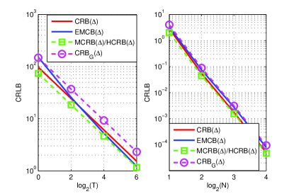
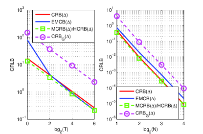
Refer to caption

Figure 5: Left: CRLBs vs. T𝑇T, M=6𝑀6M=6, N=3𝑁3N=3; right: CRLBs vs. N𝑁N, M=6𝑀6M=6, T=2𝑇2T=2. Both under K-distributed clutter.

Refer to caption

Figure 6: Left: CRLBs vs. T𝑇T, M=6𝑀6M=6, N=3𝑁3N=3; right: CRLBs vs. N𝑁N, M=6𝑀6M=6, T=2𝑇2T=2. Both under t-distributed clutter.

In Fig. 7, we inspect the impact of the texture parameters on the CRLBs under K-distributed clutter, and in Fig. 8 under t-distributed clutter, by plotting, in the left part of both figures, the CRLBs versus a𝑎a under fixed b𝑏b, and in the right versus b𝑏b under fixed a𝑎a (CRBG(Δ)subscriptCRBGΔ\text{CRB}_{\text{G}}(\Delta) is also plotted in all the four cases for comparison). The results are in exact accordance with what we have discussed in Subsection 5.5, that for both clutter distributions, the CRLBs increase with a𝑎a and remain indifferent to the change of b𝑏b. It is notable that the EMCB under K-distributed clutter, whose relationship with a𝑎a and b𝑏b has not been analytically established, also follows the same rule as the other CRLBs.
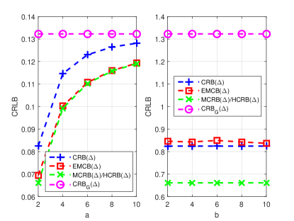
Refer to caption

Figure 7: Left: CRLBs vs. a𝑎a; right: CRLBs vs. b𝑏b. Both under K-distributed clutter.

Refer to caption

Figure 8: Left: CRLBs vs. a𝑎a; right: CRLBs vs. b𝑏b. Both under t-distributed clutter.

In Fig. 9, we verify, under both K-distributed and t-distributed clutters, our proposed analytical expressions of the ARL in Eqs. (66) and (70) (denoted in the figure by δ2subscript𝛿2\delta_{2} and δ3subscript𝛿3\delta_{3}, respectively) by plotting them versus the SCR together with the exact ARL (denoted in the figure by δ1subscript𝛿1\delta_{1}), which is numerically obtained by the approach that we proposed in [34] without any approximation. The figure shows clearly that the values of the three curves essentially coincide in asymptotic cases (above 0 dB in the context) for both distributions of clutter.
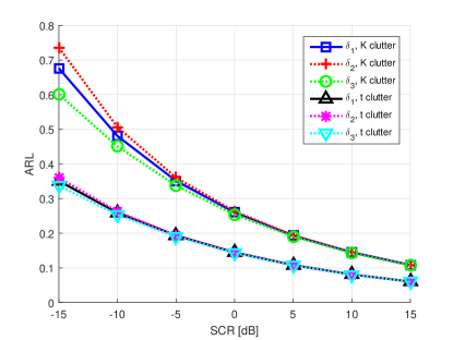
Refer to caption

Figure 9: ARL vs. SCR, M=6, N=8, under K-distributed and t-distributed clutters.

In Figs. 10 and 11, we investigate the impact of the texture parameters a𝑎a and b𝑏b on the ARL under K-distributed and t-distributed clutters, respectively. Again, we fix one of the two parameters and vary the other, and compare the resulting ARLs. One can see from these figures that δ𝛿\delta increases with a𝑎a, but remains invariant w.r.t. changes in b𝑏b, as discussed in Subsection 6.6. We also plot the ARL under Gaussian clutter for comparison, which upper-bounds all the ARL results obtained under the various SIRP clutter models considered. In fact we can say, as a direct generalization to the conclusion in [72], that for given noise power, the targets under Gaussian noise are the most difficult to be correctly resolved.
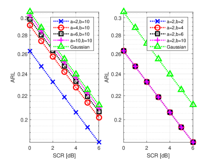
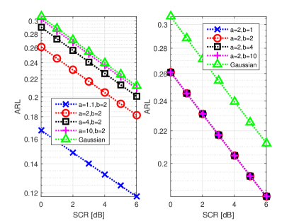
Refer to caption

Figure 10: ARL vs. SCR. Left: varying a𝑎a, fixed b𝑏b; right: varying b𝑏b, fixed a𝑎a. Both with M=6𝑀6M=6 and N=8𝑁8N=8 under K-distributed clutter.

Refer to caption

Figure 11: ARL vs. SCR. Left: varying a𝑎a, fixed b𝑏b; right: varying b𝑏b, fixed a𝑎a. Both with M=6𝑀6M=6 and N=8𝑁8N=8 under t-distributed clutter.

Finally, in Fig. 12 we inspect the respective impact of the power of the two targets on the ARL, by plotting the exact ARL (denoted by δ1subscript𝛿1\delta_{1}) and the analytical ARL in Eqs. (66) (denoted by δ2subscript𝛿2\delta_{2}) for both distributions of clutter, with the power (represented by the absolute value of the RCS factor) of one of the sources fixed and the other varying. From the figure one may observe that, while the ARL decreases with an increasing |α2|subscript𝛼2|\alpha_{2}|, it is independent of the value of |α1|subscript𝛼1|\alpha_{1}|. One may also gain insight into this from our expression in Eq. (65a), which is only dependent on |α2|subscript𝛼2|\alpha_{2}|. This follows from the fact that in our model we consider the DOD/DOA of the first source to be known, and the second unknown. Thus, increasing the power of the known source is of no avail in meliorating the resolvability of the sources, and the ARL depends solely on the concrete value of the power of the unknown source, rather than the relative ratio between the power of the two sources.
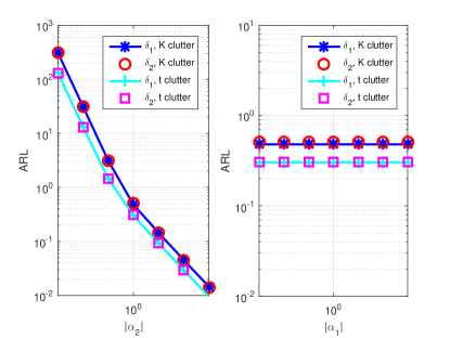
Refer to caption

Figure 12: Left: ARL vs. |α2|subscript𝛼2|\alpha_{2}|, |α1|=1subscript𝛼11|\alpha_{1}|=1; right: ARL vs. |α1|subscript𝛼1|\alpha_{1}|, |α2|=1subscript𝛼21|\alpha_{2}|=1. Both with M=6𝑀6M=6 and N=8𝑁8N=8, under K-distributed and t-distributed clutters.

8 Conclusion

This paper is dedicated to a systematical investigation into the target estimation and target resolvability problem in a MIMO context under SIRP clutter. We first devised, employing the stepwise numerical concentration approach, two independent but interconnected algorithms, the IMLE and the IMAPE, to deal with the estimation problem of the target spacing. Simulations show that both of our algorithms require only a few iterations to attain convergence, and lead to significantly superior performance than the conventional ML approach.

Next, we derived various CRLBs w.r.t. the target spacing as measures of performance for our algorithms, and analytically compared their relationships. Furthermore, by analytically investigating the effects of the texture parameters on the CRLBs, we found that they all have a positive correlation with the shape parameter, but are all independent of the scale parameter.

We then turned to the resolvability problem, namely, the ARL of two closely-spaced targets. Based on the non-matrix form expression of the CRB w.r.t. the target spacing, which was derived as a by-product, we obtained two analytical expressions for the ARL. We then analyzed the effects of the texture parameters on the ARL, which is analogous to their effect on the CRLBs. Our analytical findings on the CRLBs and the ARL are also numerically corroborated by simulations.

Appendix A Derivation of the Analytical CRB(Δ)CRBΔ\text{CRB}(\Delta)

We follow the same procedure as in Subsection 5.1 to rederive CRB(Δ)CRBΔ\text{CRB}(\Delta) based on the model Eq. (60), from which the FIM obtained has exactly the same block structure as shown in Eq. (27). The elements of its parameter block of interest 𝚽superscript𝚽\boldsymbol{\Phi}^{\prime} have the following expressions:

ϕ11superscriptsubscriptitalic-ϕ11\displaystyle\phi_{11}^{\prime} =\displaystyle= 2κ|α2|2N(γ224Δγ~23+4Δ2γ33)2𝜅superscriptsubscript𝛼22𝑁subscript𝛾224Δsubscript~𝛾234superscriptΔ2subscript𝛾33\displaystyle\frac{2\kappa|\alpha_{2}|^{2}}{N}\left(\gamma_{22}-4\Delta\widetilde{\gamma}_{23}+4\Delta^{2}\gamma_{33}\right) (A.73a)
ϕ22superscriptsubscriptitalic-ϕ22\displaystyle\phi_{22}^{\prime} =\displaystyle= ϕ33=2κNγ11,superscriptsubscriptitalic-ϕ332𝜅𝑁subscript𝛾11\displaystyle\phi_{33}^{\prime}=\frac{2\kappa}{N}\gamma_{11}, (A.73b)
ϕ44superscriptsubscriptitalic-ϕ44\displaystyle\phi_{44}^{\prime} =\displaystyle= ϕ55=2κN(γ112Δγ~12+Δ2γ22\displaystyle\phi_{55}^{\prime}=\frac{2\kappa}{N}\big{(}\gamma_{11}-2\Delta\widetilde{\gamma}_{12}+\Delta^{2}\gamma_{22} (A.73c)
2Δ2γ¯132Δ3γ~23+Δ4γ33),\displaystyle-2\Delta^{2}\overline{\gamma}_{13}-2\Delta^{3}\widetilde{\gamma}_{23}+\Delta^{4}\gamma_{33}\big{)},
ϕ12superscriptsubscriptitalic-ϕ12\displaystyle\phi_{12}^{\prime} =\displaystyle= ϕ21=2κN(α¯2γ~12α~2γ¯122Δα¯2γ¯13\displaystyle\phi_{21}^{\prime}=\frac{2\kappa}{N}\big{(}-\overline{\alpha}_{2}\widetilde{\gamma}_{12}-\widetilde{\alpha}_{2}\overline{\gamma}_{12}-2\Delta\overline{\alpha}_{2}\overline{\gamma}_{13} (A.73d)
+2Δα~2γ~13),\displaystyle+2\Delta\widetilde{\alpha}_{2}\widetilde{\gamma}_{13}\big{)},
ϕ13superscriptsubscriptitalic-ϕ13\displaystyle\phi_{13}^{\prime} =\displaystyle= ϕ31=2κN(α¯2γ¯12α~2γ~122Δα¯2γ~13\displaystyle\phi_{31}^{\prime}=\frac{2\kappa}{N}\big{(}\overline{\alpha}_{2}\overline{\gamma}_{12}-\widetilde{\alpha}_{2}\widetilde{\gamma}_{12}-2\Delta\overline{\alpha}_{2}\widetilde{\gamma}_{13} (A.73e)
2Δα~2γ¯13),\displaystyle-2\Delta\widetilde{\alpha}_{2}\overline{\gamma}_{13}\big{)},
ϕ14superscriptsubscriptitalic-ϕ14\displaystyle\phi_{14}^{\prime} =\displaystyle= ϕ41=2κN(α¯2γ~12α~2γ¯12+Δα¯2γ22\displaystyle\phi_{41}^{\prime}=\frac{2\kappa}{N}\big{(}-\overline{\alpha}_{2}\widetilde{\gamma}_{12}-\widetilde{\alpha}_{2}\overline{\gamma}_{12}+\Delta\overline{\alpha}_{2}\gamma_{22} (A.73f)
2Δα¯2γ¯13+2Δα~2γ~13Δ2α~2γ¯232Δsubscript¯𝛼2subscript¯𝛾132Δsubscript~𝛼2subscript~𝛾13superscriptΔ2subscript~𝛼2subscript¯𝛾23\displaystyle-2\Delta\overline{\alpha}_{2}\overline{\gamma}_{13}+2\Delta\widetilde{\alpha}_{2}\widetilde{\gamma}_{13}-\Delta^{2}\widetilde{\alpha}_{2}\overline{\gamma}_{23}
3Δ2α¯2γ~23+2Δ3α¯2γ33),\displaystyle-3\Delta^{2}\overline{\alpha}_{2}\widetilde{\gamma}_{23}+2\Delta^{3}\overline{\alpha}_{2}\gamma_{33}\big{)},
ϕ15superscriptsubscriptitalic-ϕ15\displaystyle\phi_{15}^{\prime} =\displaystyle= ϕ51=2κN(α¯2γ¯12α~2γ~12+Δα~2γ22\displaystyle\phi_{51}^{\prime}=\frac{2\kappa}{N}\big{(}\overline{\alpha}_{2}\overline{\gamma}_{12}-\widetilde{\alpha}_{2}\widetilde{\gamma}_{12}+\Delta\widetilde{\alpha}_{2}\gamma_{22} (A.73g)
2Δα¯2γ~132Δα~2γ¯13+Δ2α¯2γ¯232Δsubscript¯𝛼2subscript~𝛾132Δsubscript~𝛼2subscript¯𝛾13superscriptΔ2subscript¯𝛼2subscript¯𝛾23\displaystyle-2\Delta\overline{\alpha}_{2}\widetilde{\gamma}_{13}-2\Delta\widetilde{\alpha}_{2}\overline{\gamma}_{13}+\Delta^{2}\overline{\alpha}_{2}\overline{\gamma}_{23}
3Δ2α~2γ~23+2Δ3α~2γ33),\displaystyle-3\Delta^{2}\widetilde{\alpha}_{2}\widetilde{\gamma}_{23}+2\Delta^{3}\widetilde{\alpha}_{2}\gamma_{33}\big{)},
ϕ23superscriptsubscriptitalic-ϕ23\displaystyle\phi_{23}^{\prime} =\displaystyle= ϕ32=ϕ45=ϕ54=0,superscriptsubscriptitalic-ϕ32superscriptsubscriptitalic-ϕ45superscriptsubscriptitalic-ϕ540\displaystyle\phi_{32}^{\prime}=\phi_{45}^{\prime}=\phi_{54}^{\prime}=0, (A.73h)
ϕ24superscriptsubscriptitalic-ϕ24\displaystyle\phi_{24}^{\prime} =\displaystyle= ϕ42=ϕ35=ϕ53superscriptsubscriptitalic-ϕ42superscriptsubscriptitalic-ϕ35superscriptsubscriptitalic-ϕ53\displaystyle\phi_{42}^{\prime}=\phi_{35}^{\prime}=\phi_{53}^{\prime} (A.73i)
=\displaystyle= 2κN(γ11Δγ~12Δ2γ¯13),2𝜅𝑁subscript𝛾11Δsubscript~𝛾12superscriptΔ2subscript¯𝛾13\displaystyle\frac{2\kappa}{N}\left(\gamma_{11}-\Delta\widetilde{\gamma}_{12}-\Delta^{2}\overline{\gamma}_{13}\right),
ϕ25superscriptsubscriptitalic-ϕ25\displaystyle\phi_{25}^{\prime} =\displaystyle= ϕ52=ϕ34=ϕ43superscriptsubscriptitalic-ϕ52superscriptsubscriptitalic-ϕ34superscriptsubscriptitalic-ϕ43\displaystyle\phi_{52}^{\prime}=-\phi_{34}^{\prime}=-\phi_{43}^{\prime} (A.73j)
=\displaystyle= 2κN(Δγ¯12+Δ2γ~13),2𝜅𝑁Δsubscript¯𝛾12superscriptΔ2subscript~𝛾13\displaystyle\frac{2\kappa}{N}\left(-\Delta\overline{\gamma}_{12}+\Delta^{2}\widetilde{\gamma}_{13}\right),

in which

γij=𝝆iH𝚼𝝆j,i,j=1,2,3,formulae-sequencesubscript𝛾𝑖𝑗superscriptsubscript𝝆𝑖𝐻𝚼subscript𝝆𝑗𝑖𝑗123\gamma_{ij}=\boldsymbol{\rho}_{i}^{H}\boldsymbol{\Upsilon}\boldsymbol{\rho}_{j},\quad i,j=1,2,3, (A.74)

where 𝝆i=[𝝆iT(1),,𝝆iT(T)]Tsubscript𝝆𝑖superscriptsuperscriptsubscript𝝆𝑖𝑇1superscriptsubscript𝝆𝑖𝑇𝑇𝑇\boldsymbol{\rho}_{i}=[\boldsymbol{\rho}_{i}^{T}(1),\dots,\boldsymbol{\rho}_{i}^{T}(T)]^{T}, 𝝆j=[𝝆jT(1),,𝝆jT(T)]Tsubscript𝝆𝑗superscriptsuperscriptsubscript𝝆𝑗𝑇1superscriptsubscript𝝆𝑗𝑇𝑇𝑇\boldsymbol{\rho}_{j}=[\boldsymbol{\rho}_{j}^{T}(1),\dots,\boldsymbol{\rho}_{j}^{T}(T)]^{T}, and 𝚼=𝑰T𝚺1𝚼tensor-productsubscript𝑰𝑇superscript𝚺1\boldsymbol{\Upsilon}=\boldsymbol{I}_{T}\otimes\boldsymbol{\Sigma}^{-1}. The symbols 𝚽superscript𝚽\boldsymbol{\Phi}^{\prime} and ϕijsuperscriptsubscriptitalic-ϕ𝑖𝑗\phi_{ij}^{\prime} are used for these to be distinguished from their parallels 𝚽𝚽\boldsymbol{\Phi} and ϕijsubscriptitalic-ϕ𝑖𝑗\phi_{ij} derived in Subsection 5.1 based on the original model.

Let us introduce the following compact block matrix representation of 𝚽superscript𝚽\boldsymbol{\Phi}^{\prime}:

𝚽=[ϕ11𝝋T𝝋𝛀],superscript𝚽bold-′delimited-[]superscriptsubscriptitalic-ϕ11superscript𝝋𝑇𝝋𝛀\boldsymbol{\boldsymbol{\Phi}^{\prime}}=\left[\begin{array}[]{cc}\phi_{11}^{\prime}&\boldsymbol{\varphi}^{T}\\ \boldsymbol{\varphi}&\boldsymbol{\Omega}\end{array}\right], (A.75)

in which 𝝋=[ϕ12,ϕ13,ϕ14,ϕ15]T𝝋superscriptsuperscriptsubscriptitalic-ϕ12superscriptsubscriptitalic-ϕ13superscriptsubscriptitalic-ϕ14superscriptsubscriptitalic-ϕ15𝑇\boldsymbol{\varphi}=[\phi_{12}^{\prime},\ \phi_{13}^{\prime},\ \phi_{14}^{\prime},\ \phi_{15}^{\prime}]^{T}, and

𝛀=[𝛀1𝛀2𝛀2T𝛀3],𝛀delimited-[]subscript𝛀1subscript𝛀2superscriptsubscript𝛀2𝑇subscript𝛀3\boldsymbol{\Omega}=\left[\begin{array}[]{cc}\boldsymbol{\Omega}_{1}&\boldsymbol{\Omega}_{2}\\ \boldsymbol{\Omega}_{2}^{T}&\boldsymbol{\Omega}_{3}\end{array}\right], (A.76)

where 𝛀1=ϕ22𝑰2subscript𝛀1superscriptsubscriptitalic-ϕ22subscript𝑰2\boldsymbol{\Omega}_{1}=\phi_{22}^{\prime}\boldsymbol{I}_{2}, 𝛀3=ϕ44𝑰2subscript𝛀3superscriptsubscriptitalic-ϕ44subscript𝑰2\boldsymbol{\Omega}_{3}=\phi_{44}^{\prime}\boldsymbol{I}_{2}, and

𝛀2=[ϕ24ϕ25ϕ25ϕ24].subscript𝛀2delimited-[]superscriptsubscriptitalic-ϕ24superscriptsubscriptitalic-ϕ25superscriptsubscriptitalic-ϕ25superscriptsubscriptitalic-ϕ24\boldsymbol{\Omega}_{2}=\left[\begin{array}[]{cc}\phi_{24}^{\prime}&\phi_{25}^{\prime}\\ -\phi_{25}^{\prime}&\phi_{24}^{\prime}\end{array}\right]. (A.77)

By employing the block matrix inversion lemma [73] on 𝚽superscript𝚽\boldsymbol{\Phi}^{\prime} and on 𝛀𝛀\boldsymbol{\Omega} consecutively, we obtain:

CRB(Δ)=[𝚽1]1,1=ϕ111ϕ11𝝋T𝛀1𝝋,CRBΔsubscriptdelimited-[]superscript𝚽111superscriptsubscriptitalic-ϕ111superscriptsubscriptitalic-ϕ11superscript𝝋𝑇superscript𝛀1𝝋\text{CRB}\left(\Delta\right)=\left[\boldsymbol{\Phi}^{\prime-1}\right]_{1,1}=\frac{\phi_{11}^{\prime}}{1-\phi_{11}^{\prime}\boldsymbol{\varphi}^{T}\boldsymbol{\Omega}^{-1}\boldsymbol{\varphi}}, (A.78)

in which

𝛀1=[𝚯1𝚯2𝚯3𝚯4],superscript𝛀1delimited-[]subscript𝚯1subscript𝚯2subscript𝚯3subscript𝚯4\boldsymbol{\Omega}^{-1}=\left[\begin{array}[]{cc}\boldsymbol{\Theta}_{1}&\boldsymbol{\Theta}_{2}\\ \boldsymbol{\Theta}_{3}&\boldsymbol{\Theta}_{4}\end{array}\right], (A.79)

where

𝚯1=subscript𝚯1absent\displaystyle\boldsymbol{\Theta}_{1}= (𝛀1𝛀2𝛀31𝛀2T)1,superscriptsubscript𝛀1subscript𝛀2superscriptsubscript𝛀31superscriptsubscript𝛀2𝑇1\displaystyle\left(\boldsymbol{\Omega}_{1}-\boldsymbol{\Omega}_{2}\boldsymbol{\Omega}_{3}^{-1}\boldsymbol{\Omega}_{2}^{T}\right)^{-1}, (A.80a)
𝚯2=subscript𝚯2absent\displaystyle\boldsymbol{\Theta}_{2}= 𝛀11𝛀2(𝛀3𝛀2T𝛀11𝛀2)1,superscriptsubscript𝛀11subscript𝛀2superscriptsubscript𝛀3superscriptsubscript𝛀2𝑇superscriptsubscript𝛀11subscript𝛀21\displaystyle-\boldsymbol{\Omega}_{1}^{-1}\boldsymbol{\Omega}_{2}\left(\boldsymbol{\Omega}_{3}-\boldsymbol{\Omega}_{2}^{T}\boldsymbol{\Omega}_{1}^{-1}\boldsymbol{\Omega}_{2}\right)^{-1}, (A.80b)
𝚯3=subscript𝚯3absent\displaystyle\boldsymbol{\Theta}_{3}= 𝛀31𝛀2T(𝛀1𝛀2𝛀31𝛀2T)1,superscriptsubscript𝛀31superscriptsubscript𝛀2𝑇superscriptsubscript𝛀1subscript𝛀2superscriptsubscript𝛀31superscriptsubscript𝛀2𝑇1\displaystyle-\boldsymbol{\Omega}_{3}^{-1}\boldsymbol{\Omega}_{2}^{T}\left(\boldsymbol{\Omega}_{1}-\boldsymbol{\Omega}_{2}\boldsymbol{\Omega}_{3}^{-1}\boldsymbol{\Omega}_{2}^{T}\right)^{-1}, (A.80c)
𝚯4=subscript𝚯4absent\displaystyle\boldsymbol{\Theta}_{4}= (𝛀3𝛀2T𝛀11𝛀2)1;superscriptsubscript𝛀3superscriptsubscript𝛀2𝑇superscriptsubscript𝛀11subscript𝛀21\displaystyle\left(\boldsymbol{\Omega}_{3}-\boldsymbol{\Omega}_{2}^{T}\boldsymbol{\Omega}_{1}^{-1}\boldsymbol{\Omega}_{2}\right)^{-1}; (A.80d)

are 2×2222\times 2 matrices, and 𝛀11superscriptsubscript𝛀11\boldsymbol{\Omega}_{1}^{-1} and 𝛀31superscriptsubscript𝛀31\boldsymbol{\Omega}_{3}^{-1} are simply 1/ϕ22𝑰21superscriptsubscriptitalic-ϕ22subscript𝑰21/\phi_{22}^{\prime}\boldsymbol{I}_{2} and 1/ϕ44𝑰21superscriptsubscriptitalic-ϕ44subscript𝑰21/\phi_{44}^{\prime}\boldsymbol{I}_{2}, respectively.

After calculation, we obtain the analytical expression for CRB(Δ)CRBΔ\text{CRB}\left(\Delta\right) from Eq. (30) as:

CRB(Δ)=1ϕ11+Q,CRBΔ1superscriptsubscriptitalic-ϕ11𝑄\text{CRB}\left(\Delta\right)=\frac{1}{\phi_{11}^{\prime}+Q}, (A.81)

in which Q=(ϕ44ϕ122+ϕ44ϕ132+ϕ22ϕ142+ϕ22ϕ1522ϕ24ϕ12ϕ142ϕ25ϕ12ϕ15+2ϕ25ϕ13ϕ152ϕ24ϕ13ϕ15)/(ϕ242+ϕ252ϕ22ϕ44)𝑄superscriptsubscriptitalic-ϕ44superscriptsubscriptitalic-ϕ122superscriptsubscriptitalic-ϕ44superscriptsubscriptitalic-ϕ132superscriptsubscriptitalic-ϕ22superscriptsubscriptitalic-ϕ142superscriptsubscriptitalic-ϕ22superscriptsubscriptitalic-ϕ1522superscriptsubscriptitalic-ϕ24superscriptsubscriptitalic-ϕ12superscriptsubscriptitalic-ϕ142superscriptsubscriptitalic-ϕ25superscriptsubscriptitalic-ϕ12superscriptsubscriptitalic-ϕ152superscriptsubscriptitalic-ϕ25superscriptsubscriptitalic-ϕ13superscriptsubscriptitalic-ϕ152superscriptsubscriptitalic-ϕ24superscriptsubscriptitalic-ϕ13superscriptsubscriptitalic-ϕ15superscriptsubscriptitalic-ϕ242superscriptsubscriptitalic-ϕ252superscriptsubscriptitalic-ϕ22superscriptsubscriptitalic-ϕ44Q=(\phi_{44}^{\prime}\phi_{12}^{\prime 2}+\phi_{44}^{\prime}\phi_{13}^{\prime 2}+\phi_{22}^{\prime}\phi_{14}^{\prime 2}+\phi_{22}^{\prime}\phi_{15}^{\prime 2}-2\phi_{24}^{\prime}\phi_{12}^{\prime}\phi_{14}^{\prime}-2\phi_{25}^{\prime}\phi_{12}^{\prime}\phi_{15}^{\prime}+2\phi_{25}^{\prime}\phi_{13}^{\prime}\phi_{15}^{\prime}-2\phi_{24}^{\prime}\phi_{13}^{\prime}\phi_{15}^{\prime})/(\phi_{24}^{\prime 2}+\phi_{25}^{\prime 2}-\phi_{22}^{\prime}\phi_{44}^{\prime}).

References

References

  • [1] E. Fishler, MIMO radar: an idea whose time has come, in: Proc. IEEE Radar Conference, Philadelphia, PA, 2004, pp. 71–78.
  • [2] J. Li, P. Stoica, MIMO radar Signal Processing, Wiley-Interscience, New York, 2008.
  • [3] I. Bekkerman, J. Tabrikian, Target detection and localization using MIMO radars and sonars, IEEE Trans. Signal Processing 54 (10) (2006) 3873–3883.
  • [4] C.-Y. Chen, P. P. Vaidyanathan, MIMO radar space-time adaptive processing using prolate spheroidal wave functions, IEEE Trans. Signal Processing 56 (2) (2008) 623–635.
  • [5] A. Haimovich, R. Blum, L. Cimini, MIMO radar with widely separated antennas, IEEE Signal Processing Magazine 25 (2008) 116–129.
  • [6] J. Li, P. Stoica, MIMO radar with colocated antennas, IEEE Signal Processing Magazine 24 (5) (2007) 106–114.
  • [7] M. Jin, G. Liao, J. Li, Joint DOD and DOA estimation for bistatic MIMO radar, Signal Processing 89 (2) (2009) 244–251.
  • [8] R. Boyer, Performance bounds and angular resolution limit for the moving co-located MIMO radar, IEEE Trans. Signal Processing 59 (4) (2011) 1539–1552.
  • [9] M. N. El Korso, R. Boyer, A. Renaux, S. Marcos, Statistical resolution limit for source localization with clutter interference in a MIMO radar context, IEEE Trans. Signal Processing 60 (5) (2012) 987–992.
  • [10] M. N. El Korso, F. Pascal, M. Pesavento, On the resolvability of closely spaced targets using a colocated MIMO radar, in: Proc. 46th Asilomar Conference on Signals, Systems and Computers, Pacific Grove, 2012, invited paper.
  • [11] T.-Q. Xia, Joint diagonalization based DOD and DOA estimation for bistatic MIMO radar, Signal Processing 108 (2015) 159–166.
  • [12] M. Einemo, H. C. So, Weighted least squares algorithm for target localization in distributed MIMO radar, Signal Processing 115 (2015) 144–150.
  • [13] S. Hong, X. Wan, H. Ke, Spatial difference smoothing for coherent sources location in MIMO radar, Signal Processing 109 (2015) 69–83.
  • [14] Y.-H. Tang, X.-F. Ma, W.-X. Sheng, Y. Han, Transmit beamforming for DOA estimation based on Cramer-Rao bound optimization in subarray MIMO radar, Signal Processing 101 (2014) 42–51.
  • [15] J. B. Billingsley, Ground clutter measurements for surface-sited radar, Tech. Rep. 780, Massachusetts Inst. Technol., Cambridge, MA (Feb. 1993).
  • [16] F. Gini, M. V. Greco, M. Diani, L. Verrazzani, Performance analysis of two adaptive radar detectors against non-Gaussian real sea clutter data, IEEE Trans. Aerosp. Electron. Syst. 36 (4) (2000) 1429–1439.
  • [17] K. Yao, Spherically invariant random processes: Theory and applications, in: V. K. B. et al. (Ed.), Communications, Information and Network Security, 2002, pp. 315–332.
  • [18] K. Yao, A representation theorem and its applications to spherically invariant random processes, IEEE Trans. Inf. Theory 19 (5) (1973) 600–608.
  • [19] M. Rangaswamy, D. D. Weiner, A. Ozturk, Non-Gaussian vector identification using spherically invariant random processes, IEEE Trans. Aerosp. Electron. Syst. 29 (1) (1993) 111–124.
  • [20] E. Jakeman, P. N. Pusey, A model for non-Rayleigh sea echo, IEEE Trans. Antennas Propag. 24 (6) (1976) 806–814.
  • [21] E. Conte, G. Ricci, Performance prediction in compound-Gaussian clutter, IEEE Trans. Aerosp. Electron. Syst. 30 (2) (1994) 611–616.
  • [22] F. Gini, Sub-optimum coherent radar detection in a mixture of K-distributed and Gaussian clutter, IEE Proceedings - Radar, Sonar and Navigation 114 (1) (1997) 39–48.
  • [23] M. Greco, F. Bordoni, F. Gini, X-band see-clutter nonstationarity: Influence of long waves, IEEE J. Ocean. Eng. 29 (2) (2004) 269–283.
  • [24] C. Liu, D. B. Rubin, ML estimation of the t distribution using EM and its extensions, ECM and ECME, Statistica Sinica 5 (1995) 19–39.
  • [25] F. Pascal, Y. Chitour, J.-P. Ovarlez, P. Forster, Covariance structure maximum-likelihood estimates in compound Gaussian noise: Existence and algorithm analysis, IEEE Trans. Signal Processing 56 (1) (2008) 34–48.
  • [26] J. Wang, A. Dogandžić, A. Nehorai, Maximum likelihood estimation of compound Gaussian clutter and taget parameters, IEEE Trans. Signal Processing 54 (10) (2006) 3884–3897.
  • [27] Y. Chitour, F. Pascal, Exact maximum-likelihood estimates for SIRV covariance matrix: Existence and algorithm analysis, IEEE Trans. Signal Processing 56 (10) (2008) 4563–4573.
  • [28] P. Lombardo, C. J. Oliver, Estimation of texture parameters in K-distributed clutter, IEE Proceedings - Radar, Sonar and Navigation 141 (4) (1994) 196–204.
  • [29] M. Akcakaya, A. Nehorai, Adaptive MIMO radar design and detection in compound-Gaussian clutter, IEEE Trans. Aerosp. Electron. Syst. 47 (3) (2011) 2200–2207.
  • [30] A. Dogandžić, A. Nehorai, Generalized multivariate analysis of variance: A unified framework for signal processing in correlated noise, IEEE Signal Processing Magazine 20.
  • [31] M. Haardt, M. Pesavento, F. Röemer, M. N. El Korso, Subspace Methods and Exploitation of Special Array Structures, Electronic Reference in Signal Processing: Array and Statistical Signal Processing (M. Viberg, ed.), Vol. 3, Academic Press Library in Signal Processing, Elsevier Ltd., 2014.
  • [32] M. Pesavento, A. B. Gershman, Maximum-likelihood direction-of-arrival estimation in the presence of unknown nonuniform noise, IEEE Trans. Signal Processing 49 (7) (2001) 1310–1324.
  • [33] S. A. Vorobyov, A. B. Gershman, K. M. Wong, Maximum likelihood direction-of-arrival estimation in unknown noise fields using sparse sensor arrays, IEEE Trans. Signal Processing 53 (1) (2005) 34–43.
  • [34] X. Zhang, M. N. El Korso, M. Pesavento, MIMO radar performance analysis under K-distributed clutter, in: Proc. ICASSP, Florence, Italy, 2014, pp. 5287–5291.
  • [35] S. T. Smith, Statistical resolution limits and the complexified Cramér Rao bound, IEEE Trans. Signal Processing 53 (5) (2005) 1597–1609.
  • [36] M. Shahram, P. Milanfar, On the resolvability of sinusoids with nearby frequencies in the presence of noise, IEEE Trans. Signal Processing 53 (7) (2005) 2579–2588.
  • [37] M. N. El Korso, R. Boyer, A. Renaux, S. Marcos, Statistical resolution limit for multiple parameters of interest and for multiple signals, in: Proc. ICASSP, Dallas, TX, 2010, pp. 3602–3605.
  • [38] H. Cox, Resolving power and sensitivity to mismatch of optimum array processors, J. Acoust. Soc. 54 (3) (1973) 771–785.
  • [39] M. Shahram, P. Milanfar, Imaging below the diffraction limit: A statistical analysis, IEEE Trans. Image Processing 13 (5) (2004) 677–689.
  • [40] Z. Liu, A. Nehorai, Statistical angular resolution limit for point sources, IEEE Trans. Signal Processing 55 (11) (2007) 5521–5527.
  • [41] M. N. El Korso, R. Boyer, A. Renaux, S. Marcos, Statistical analysis of achievable resolution limit in the near field source localization context, Signal Processing 92 (2) (2012) 547–552.
  • [42] M. N. El Korso, R. Boyer, A. Renaux, S. Marcos, On the asymptotic resolvability of two point sources in known subspace interference using a GLRT-based framework, Signal Processing 92 (10) (2012) 2471–2483.
  • [43] H. B. Lee, The Cramér-Rao bound on frequency estimates of signals closely spaced in frequency, IEEE Trans. Signal Processing 40 (6) (1992) 1507–1517.
  • [44] M. N. El Korso, R. Boyer, A. Renaux, S. Marcos, Statistical resolution limit of the uniform linear cocentered orthogonal loop and dipole array, IEEE Trans. Signal Processing 59 (1) (2011) 425–431.
  • [45] X. Zhang, M. N. El Korso, M. Pesavento, On the asymptotic resolvability of far-field stochastic sources, in: Proc. EUSIPCO, Bucharest, Romania, 2012, pp. 889–893.
  • [46] X. Zhang, M. N. El Korso, M. Pesavento, Angular resolution limit for deterministic correlated sources, in: Proc. ICASSP, Vancouver, Canada, 2013, pp. 5539–5543.
  • [47] H. B. Lee, The Cramér-Rao bound on frequency estimates of signals closely spaced in frequency (unconditional case), IEEE Trans. Signal Processing 42 (6) (1994) 1569–1572.
  • [48] E. Dilaveroglu, Nonmatrix Cramér-Rao bound expressions for high-resolution frequency estimators, IEEE Trans. Signal Processing 46 (2) (1998) 463–474.
  • [49] M. Kaveh, A. J. Barabell, The statistical performance of the MUSIC and the minimum-norm algorithms in resolving plane waves in noise, IEEE Trans. Acoust., Speech, Signal Processing 34 (2) (1986) 331–341.
  • [50] S. Watts, Radar detection prediction in sea clutter using the compound K-distribution model, Proc. Inst. Electr. Eng. F 132 (7) (1985) 613–620.
  • [51] T. Nohara, S. Haykin, Canada east coast trials and the K-distribution, Proc. Inst. Electr. Eng. F 138 (2) (1991) 82–88.
  • [52] K. J. Sangston, K. R. Gerlach, Coherent detection of radar targets in a non-Gaussian background, IEEE Trans. Aerosp. Electron. Syst. 30 (2) (1994) 330–340.
  • [53] K. L. Lange, R. J. A. Little, J. M. G. Taylor, Robust statistical modeling using the t distribution, J. Amer. Stat. Assoc. 84 (408) (1989) 881–896.
  • [54] E. Jay, J.-P. Ovarlez, D. Declercq, P. Duvaut, Bayesian optimum radar detector in non-Gaussian noise, in: Proc. ICASSP, Orlando, FL, 2002, pp. 1289–1292.
  • [55] E. Jay, J.-P. Ovarlez, D. Declercq, P. Duvaut, BORD: Bayesian optimum radar detector, Signal Processing 83 (6) (2003) 1151–1162.
  • [56] E. Conte, A. D. Maio, G. Ricci, Recursive estimation of the covariance matrix of a compound-Gaussian process and its application to adaptive CFAR detection, IEEE Trans. Signal Processing 50 (8) (2002) 1908–1915.
  • [57] T. W. Anderson, An Introduction to Multivariate Statistical Analysis, 3rd Edition, Wiley-Interscience, New York, 2003.
  • [58] F. Gini, M. Greco, Covariance matrix estimation for CFAR detection in correlated heavy tailed clutter, Signal Processing 82 (12) (2002) 1847–1859.
  • [59] F. Gini, R. Reggiannini, On the use of Cramér-Rao-like bounds in the presence of random nuisance parameters, IEEE Trans. Commun. 48 (12) (2000) 2120–2126.
  • [60] R. W. Miller, C. B. Chang, A modified Cramér-Rao bound and its applications, IEEE Trans. Inform. Theory 24 (3) (1978) 398–400.
  • [61] F. Gini, R. Reggiannini, U. Mengali, The modified Cramér-Rao bound in vector parameter estimation, IEEE Trans. Commun. 46 (1) (1998) 52–60.
  • [62] I. Reuven, H. Messer, A Barankin-type lower bound on the estimation error of a hybrid parameter vector, IEEE Trans. Inform. Theory 43 (3) (1997) 1084–1093.
  • [63] T. Groves, T. Rothenberg, A note on the expected value of an inverse matrix, Biometrika 56 (3) (1969) 690–691.
  • [64] A. Papoulis, S. U. Pillai, Probability, random variables, and stochastic processes, McGraw-Hill, New York, 1965.
  • [65] M. Shahram, P. Milanfar, On the resolvability of sinusoids with nearby frequencies in the presence of noise, IEEE Trans. Signal Processing 53 (7) (2005) 2579–2585.
  • [66] A. Amar, A. Weiss, Fundamental limitations on the resolution of deterministic signals, IEEE Trans. Signal Processing 56 (11) (2008) 5309–5318.
  • [67] H. L. V. Trees, Optimum Array Processing: Part IV of Detection, Estimation, and Modulation Theory, John Wiley & Sons Inc., New York, 2002.
  • [68] P. Stoica, A. Nehorai, MUSIC, maximum likelihood and Cramer-Rao bound, IEEE Trans. Acoust., Speech, Signal Processing 37 (5) (1989) 720–741.
  • [69] E. L. Lehmann, Theory of Point Estimation, Wiley, New York, 1983.
  • [70] S. M. Kay, Fundamentals of Statistical Signal Processing : Estimation Theory, Vol. 1, Prentice Hall, NJ, 1993.
  • [71] M. Viberg, P. Stoica, B. Ottersten, Maximum likelihood array processing in spatially correlated noise fields using parameterized signals, IEEE Trans. Signal Processing 45 (4) (1997) 996–1004.
  • [72] P. Stoica, P. Babu, The Gaussian data assumption leads to the largest Cramér-Rao bound [lecture notes], IEEE Signal Processing Magazine 28 (3) (2011) 132–133.
  • [73] K. Petersen, M. Pedersen, The matrix cookbook, Citeseer.