Continuous 3D Label Stereo Matching using
Local Expansion Moves
Abstract
We present an accurate stereo matching method using local expansion moves based on graph cuts. This new move-making scheme is used to efficiently infer per-pixel 3D plane labels on a pairwise Markov random field (MRF) that effectively combines recently proposed slanted patch matching and curvature regularization terms. The local expansion moves are presented as many -expansions defined for small grid regions. The local expansion moves extend traditional expansion moves by two ways: localization and spatial propagation. By localization, we use different candidate -labels according to the locations of local -expansions. By spatial propagation, we design our local -expansions to propagate currently assigned labels for nearby regions. With this localization and spatial propagation, our method can efficiently infer MRF models with a continuous label space using randomized search. Our method has several advantages over previous approaches that are based on fusion moves or belief propagation; it produces submodular moves deriving a subproblem optimality; it helps find good, smooth, piecewise linear disparity maps; it is suitable for parallelization; it can use cost-volume filtering techniques for accelerating the matching cost computations. Even using a simple pairwise MRF, our method is shown to have best performance in the Middlebury stereo benchmark V2 and V3.
Index Terms:
Stereo Vision, 3D Reconstruction, Graph Cuts, Markov Random Fields, Discrete-Continuous Optimization.1 Introduction
Stereo vision often struggles with a bias toward reconstructing fronto-parallel surfaces, which can stem from matching cost, smoothness regularization, or even inference [5, 45].
Segment-based stereo [4] that represents disparity maps by disparity plane segments, could ease the bias issue but recovered surfaces are constrained to be piecewise planar. Recently, two breakthroughs have been independently made that overcome the fronto-parallel bias while surpassing the limitation of segment-based stereo.
One breakthrough is matching cost using slanted patch matching [5]. In this approach, the disparity of each pixel is over-parameterized by a local disparity plane
| (1) |
defined on the image domain , and the triplet is estimated for each pixel instead of directly estimating . The matching window is then slanted according to Eq. (1), which produces linearly-varying disparities within the window and thereby measures patch dissimilarity accurately even with large matching windows.
Another key invention is curvature regularization [33, 27] by tangent plane labels. Unlike second-order smoothness [45] that forms a higher-order term, this curvature regularization is nicely represented by pairwise terms like conventional (fronto-parallel) linear [19] and truncated linear models, and can handle smooth surfaces beyond planes.
Given slanted patch matching [5] and tangent-based curvature regularization [33], the use of 3D plane labels allows us to establish a new stereo model using a pairwise Markov random field (MRF) [12] that is free from the fronto-parallel bias. However, while stereo with standard 1D discrete disparity labels [42, 23, 8] can be directly solved by discrete optimizers such as graph cuts (GC) [24, 7] and belief propagation (BP) [47, 11], such approaches cannot be directly used for continuous 3D labels due to the huge or infinite label space .
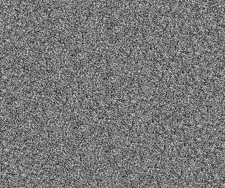
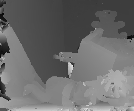
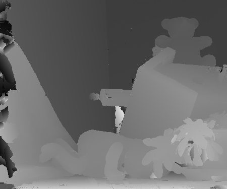
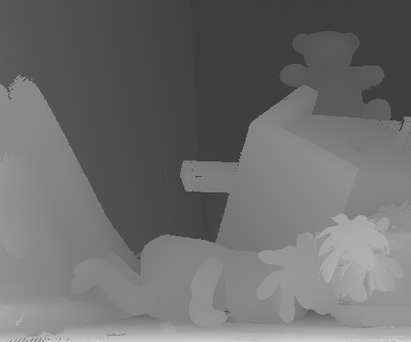
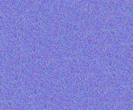
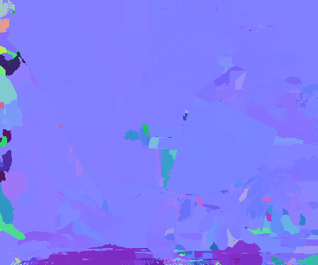
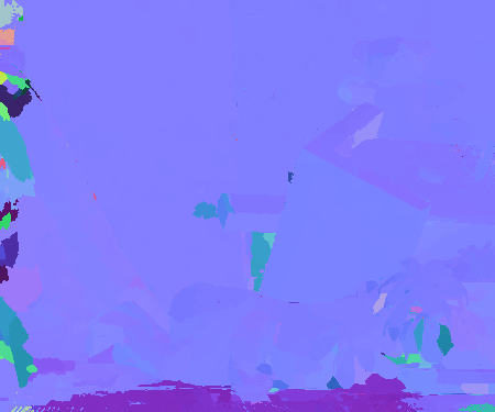

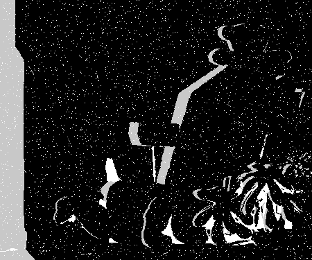
Random init.
iteration
iterations
Post-processing
To efficiently infer 3D labels, recent successful methods [5, 3, 32, 14] use PatchMatch [1, 2], an inference algorithm using spatial label propagation. In PatchMatch, each pixel is updated in raster-scan order and its refined label is propagated to next pixels as their candidate labels. Further in [3], this sequential algorithm is combined with BP yielding an efficient optimizer PMBP for pairwise MRFs. In terms of MRF optimization, however, BP is considered a sequential optimizer, which improves each variable individually keeping others conditioned at the current state. In contrast, GC improves all variables simultaneously by accounting for interactions across variables, and this global property helps optimization avoid bad local minimums [38, 45]. In order to take advantage of this and efficiently infer 3D planes by GC, it is important to use spatial propagation. Nevertheless, incorporating such spatial propagation into GC-based optimization is not straightforward, because inference using GC rather processes all nodes simultaneously, not one-by-one sequentially like PatchMatch and BP.
In this paper, we introduce a new move making scheme, local expansion moves, that enables spatial propagation in GC optimization. The local expansion moves are presented as many -expansions [8] defined for a small extent of regions at different locations. Each of this small or local -expansion tries to improve the current labels in its local region in an energy minimization manner using GC. Here, those current labels are allowed to move to a candidate label , which is given uniquely to each local -expansion in order to achieve efficient label searching. At the same time, this procedure is designed to propagate a current label in a local region for nearby pixels. For natural scenes that often exhibit locally planar structures, the joint use of local expansion moves and GC has a useful property. It allows multiple pixels in a local region to be assigned the same disparity plane by a single min-cut in order to find a smooth solution. Being able to simultaneously update multiple variables also helps to avoid being trapped at a bad local minimum.
For continuous MRF inference, fusion-based approaches using GC [25] are often employed with some heuristics to generate disparity map proposals [45, 33, 34]. Our work bridges between apparently different inference approaches of PatchMatch and GC, and can take advantage of those heuristics used in both PatchMatch and fusion based approaches leading to higher efficiency and accuracy.
The advantages of our method are as follows. 1) Our local expansion move method produces submodular moves that guarantee the optimal labeling at each min-cut (subproblem optimal), which in contrast is not guaranteed in general fusion moves [25]. 2) This optimality and spatial propagation allow randomized search, rather than employ external methods to generate plausible initial proposals as done in fusion approaches [25, 45], which may limit the possible solutions. 3) Our method achieves greater accuracy than BP [3] thanks to the good properties of GC and local expansion moves. 4) Unlike other PatchMatch based methods [5, 3, 14], our method can incorporate the fast cost filtering technique of [32]. In this manner, we can efficiently reduce the computation complexity of unary terms from to approximately , removing dependency from support window size . 5) Unlike PMBP [3], our method is well suited for parallelization using both CPU and GPU.111Although BP is usually parallelizable, PMBP differs from BP’s standard settings in that it defines label space dynamically for each pixel and propagates it; both make parallelization indeed non-trivial. With multiple CPU cores, each of our local -expansions (i.e., min-cut computations) can be individually performed in parallel. With a GPU implementation, computations of unary terms can be more efficiently performed in a parallel manner for further acceleration.
This paper is an extended version of our conference paper [39]. The extensions are summarized as follows. We add theoretical verifications on the preferability of our method for piecewise planar scenes in Sec. 3.1, and also on the subproblem optimality of our algorithm in Sec. 3.3. Furthermore, the efficiency of our algorithm is improved by two ways; In Sec. 3.3 we show the parallelizablity of our local expansion move algorithm; In Sec. 3.5 we show that the fast cost filtering technique of [32] can be used in our method. The effectiveness of both extensions is thoroughly evaluated in the experiments, and we show that even a CPU implementation of the proposed method achieves about 2.1x faster running times than our previous GPU implementation [39], with comparable or even greater accuracy. Finally, we add experimental evaluations in Sec. 4 showing that our method outperforms a fusion-based approach [33] and all the state-of-the-art methods registered in the latest Middlebury benchmark V3. Our code is publicly available online (https://github.com/t-taniai/LocalExpStereo).
2 Related work
2.1 MRF stereo methods
MRF stereo methods can be categorized into thee approaches: discrete stereo, segment-based stereo, and continuous stereo.
Discrete stereo [42, 23, 8] formulates stereo matching as a discrete multi-labeling problem, where each pixel is individually assigned one of pre-defined discrete disparity values. For this problem, many powerful discrete optimizers, such as BP [47, 11], TRW [21], and GC [24, 7], can be directly used. Successful results are shown using GC with expansion moves [8, 38]. In expansion moves, the multi-labeling problem is reduced to a sequence of binary-labeling problems, each of which can be exactly solved by GC, if only pairwise potentials meet the following submodularity of expansion moves [22, 8]:
| (2) |
Segment-based stereo [4, 41, 15, 43] assigns a 3D disparity plane for each of over-segmented image regions. Although this approach yields continuous-valued disparities, it strictly limits the reconstruction to a piecewise planar representation and is subject to the quality of initial segmentation. More recent methods alleviate these limitations by using a complex layered MRF [6], multi-scale segmentation [26], or jointly estimating segmentation [46].
The last group, to which our method belongs, is continuous stereo [45, 5, 3, 33, 32, 14], where each pixel is assigned a distinct continuous disparity value. Some methods [45, 33] use fusion moves [25], an operation that combines two solutions to make better one (binary fusion) by solving a non-submodular binary-labeling problem using QPBO-GC [22]. In this approach, a number of continuous-valued disparity maps (or so-called proposals in the literature [25]) are first generated by other external methods (e.g., segment-based stereo [45]), which are then combined as a sequence of binary fusions. Our method differs from this fusion-based approach in that we use spatial propagation and randomization search during inference, by which we only require a randomized initial solution instead of those generated by external methods. Also, binary energies produced in our method are always submodular allowing exact inference via GC (subproblem optimal). More importantly, we rather provide an efficient inference mechanism that is conceptually orthogonal to proposal generation. Thus, conventional proposal generation schemes used in fusion approaches [45, 33, 34] can be incorporated in our method for further improvements. A stereo method by Bleyer et al. [5] proposes accurate photo-consistency measures using 3D disparity planes that are inferred by PatchMatch [1, 2]. Heise et al. [14] incorporate Huber regularization into [5] using convex optimization. Besse et al. [3] point out a close relationship between PatchMatch and BP and present a unified method called PatchMatch BP (PMBP) for pairwise continuous MRFs. PMBP is probably the closest approach to ours in spirit, but we use GC instead of BP for the inference. Therefore, our method is able to take advantage of better convergence of GC [38] for achieving greater accuracy. In addition, our method allows efficient parallel computation of unary matching costs and even min-cut operations.
2.2 Cost-volume filtering
Patch-based stereo methods often use cost-volume filtering for fast implementations. Generally, computing a matching cost for a patch requires of computation, where is the size of the patch. However, given a cost-volume slice that represents pixelwise raw matching costs for a certain disparity label , the patch-based matching costs can be efficiently computed by applying a filtering to the cost map as . Here, the filter kernel represents the matching window at . If we use a constant-time filtering, each matching cost is efficiently computed in .
The box filtering can achieve by using integral image but such simple filtering flattens object boundaries. For this boundary issue, Yoon and Kweon [48] propose an adaptive support-window technique that uses the joint bilateral filtering [35] for cost filtering. Although this adaptive window technique successfully deals with the boundary issue [16], it involves of computation because of the complexity of the bilateral filtering. Recently, He et al. [13] propose a constant-time edge-aware filtering named the guided image filtering. This filtering is employed in a cost-volume filtering method of [36, 17], achieving both edge-awareness and of matching-cost computation.
In principle, stereo methods using PatchMatch inference [5, 3, 14] cannot take advantage of the cost filtering acceleration, since in those methods the candidate disparity labels are given dynamically to each pixel and we cannot make a consistent-label cost-volume slice . To this issue, Lu et al. [32] extend PatchMatch [5] to use superpixels as a unit of cost calculations. In their method, called PatchMatch filter (PMF), fast cost-volume filtering of [36, 17] is applied in small subregions and that approximately achieves of complexity. We will show in Sec. 3.5 that their subregion filtering technique can be effectively incorporated into our method, and we achieve greater accuracy than their local stereo method [32].
3 Proposed method
This section describes our proposed method. Given two input images and , our purpose is to estimate the disparities of both images.
In Sec. 3.1, we first discuss a geometric property of our model. We then define our energy function in Sec. 3.2, and describe the fundamental idea of our optimizing strategy and its properties in Sec. 3.3. The whole optimization procedure is presented in Sec. 3.4, and we further discuss a fast implementation in Sec. 3.5.
3.1 Geometric interpretation to slanted patch matching
Slanted patch matching [5] by Eq. (1) implicitly assumes that the true disparity maps are approximately piecewise linear. While it is not discussed in [5], linear disparity is exactly related to motion by planar surfaces [4, 33]. Formally, if there exists a plane in the 3D world coordinates
| (3) |
parameterized by , then motion due to this geometric plane is represented by a disparity plane
| (4) |
where and are the baseline and focal length of the stereo cameras.222Derived easily by using the perspective projection and , and the depth-disparity relation in rectified stereo. This piecewise planar assumption is reasonable as many natural scenes approximately exhibit locally planar surfaces. As we will discuss later, this fact also supports our method design as our model and inference both softly prefer piecewise linear disparity maps while having the ability to express arbitrary curved surfaces.
3.2 Formulation
We use the 3D plane label formulation to take advantage of the powerful slanted patch matching [5] and curvature regularization [33]. Here, each pixel ’s disparity is over-parameterized by a 3D plane . Therefore, we seek a mapping that assigns a disparity plane for every pixel in the left and right images. Following conventional MRF stereo methods [33, 42, 23, 8], we estimate by minimizing the following energy function based on a pairwise MRF.
| (5) |
The first term, called the data term or unary term, measures the photo-consistency between matching pixels. The disparity plane defines a warp from a pixel in one image to its correspondence in the other image. The second term is called the smoothness term or pairwise term, which penalizes discontinuity of disparities between neighboring pixel pairs . We define these terms below.
Data term
To measure photo-consistencies, we use the slanted patch matching term that has been recently proposed by [5]. The data term of in the left image is defined as
| (6) |
Here, is a square window centered at . The weight implements the adaptive support window proposed in [48]. For this we replace the bilateral filter weight used in [48, 5] with more advanced guided image filtering [13] as below.
| (7) |
Here, is a normalized color vector, and are the mean and co-variance matrix of in a local regression window , and is an identity matrix with a small positive coefficient for avoiding over-fitting. We will discuss how to efficiently compute this filtering in Sec. 3.5.
Given a disparity plane , the function in Eq. (6) measures the pixel dissimilarity between a support pixel in the window and its matching point in the right image
| (8) |
as
| (9) |
Here, represents the -component of the gray-value gradient of image , and is a factor that balances the weights of color and gradient terms. The two terms are truncated by and to increase the robustness for occluded regions. We use linear interpolation for , and a sobel filter kernel of for . When the data term is defined on the right image, we swap and in Eqs. (7) and (9), and add the disparity value in Eq. (8).
Smoothness term
For the smoothness term, we use a curvature-based, second-order smoothness regularization term [33] defined as
| (10) |
Here, is a contrast-sensitive weight defined as
| (11) |
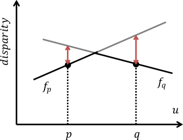
where is a user-defined parameter. The is a small constant value that gives a lower bound to the weight to increase the robustness to image noise. The function penalizes the discontinuity between and in terms of disparity as
| (12) |
where . The first term in Eq. (12) measures the difference between and by their disparity values at , and the second term is defined similarly at . We visualize as red arrows in Fig. 2 (a). The is truncated at to allow sharp jumps in disparity at depth edges.

(a)
(b)
Notice that when is forced; therefore, the smoothness term naturally extends the traditional truncated linear model [8], although the latter has a fronto-parallel bias and should be avoided [45, 33]. Also, as shown in Fig. 2 (b), this term becomes zero when . This enforces piecewise linear disparity maps and so piecewise planar object surfaces. Furthermore, this term satisfies the following property for taking advantage of GC.

Proof.
See [33] and also Appendix A. ∎
3.3 Local expansion moves
In this section, we describe the fundamental idea of our method, local expansion moves, as the main contribution of this paper. We first briefly review the original expansion move algorithm [8], and then describe how we extend it for efficiently optimizing continuous MRFs.
The expansion move algorithm [8] is a discrete optimization method for pairwise MRFs of Eq. (5), which iteratively solves a sequence of the following binary labeling problems
| (13) |
for all possible candidate labels . Here, the binary variable for each pixel is assigned either its current label or a candidate label . If all the pairwise terms in meet the condition of Eq. (2), then the binary energies in Eq. (13) are submodular and this minimization can thus be exactly solved via GC [8] (subproblem optimal). Here, it is guaranteed that the energy does not increase: . However, the label space in our setting is a three dimensional continuous space ; therefore, such an exhaustive approach cannot be employed.
Our local expansion moves extend traditional expansion moves by two ways; localization and spatial propagation. By localization, we use different candidate labels depending on the locations of pixels in Eq. (13), rather than using the same label for all pixels. This is reasonable because the distributions of disparities should be different from location to location, therefore the selection of candidate labels should be accordingly different. By spatial propagation, we incorporate label propagation similar to the PatchMatch inference [1, 2, 5] into GC optimization, and propagate currently assigned labels to nearby pixels via GC. The assumption behind this propagation is that, if a good label is assigned to a pixel, this label is likely a good estimate for nearby pixels as well. The localization and spatial propagation together make it possible for us to use a powerful randomized search scheme, where we no longer need to produce initial solution proposals as usually done in the fusion based approach [25]. Below we provide the detailed descriptions of our algorithm.
Local -expansions for spatial propagation
We first define a grid structure that divides the image domain into grid regions , which are indexed by 2D integer coordinates . We refer to each of these grid regions as a cell. We in this paper simply assume regular square cells, but this could be extended to use superpixels [18, 29, 40]. At a high level, the size of cells balances between the level of localization and the range of spatial propagation. Smaller sizes of cells can achieve finer localization but result in shorter ranges of spatial propagation. Later in Sec 3.4 we introduce different sizes of multiple grid structures for balancing these two factors well, but for now let us focus on using one grid structure.
Given a grid structure, we define a local -expansion at each cell , which we specifically denote as -expansion. We further define two types of regions for each -expansion: its center region and expansion region
| (14) |
i.e., cells consisting of the center region and its eight neighbor cells.
In the middle part of Fig. 3, we focus on an expansion region and illustrate how an -expansion works. We first randomly select a pixel from the center region , and take its currently assigned label as . We then make a candidate label by perturbing this current label as . Finally, we update the current labels of pixels in the expansion region , by choosing either their current labels or the candidate label . Here, similarly to Eq. (13), we update the partial labeling by minimizing with binary variables: for , and for . Consequently, we obtain an improved solution as its minimizer with a lower or equal energy.
Notice that making the expansion region larger than the label selection region is the key idea for achieving spatial propagation. We can see this since, in an -expansion without perturbation (), a current label in the center region can be propagated for its nearby pixels in as the candidate label .
We use this -expansion iteratively as shown in Algorithm 1. Similarly to the PatchMatch algorithm [1], this iterative algorithm has propagation (lines 1–4) and refinement (lines 9–14) steps. In the propagation step, we apply -expansions without perturbation to propagate labels from for . In the refinement step, we apply -expansions with an exponentially decreasing perturbation-size to refine the labels. Here, propagation and refinement can be seen as heuristic proposers of a candidate label that is expectedly a good estimate for the region or even its neighborhood . Our local expansion move method is conceptually orthogonal to any such heuristics for generating . As such an example, we in lines 5–8 use a RANSAC proposer by following conventional proposal generation schemes used in fusion-based methods [45, 33]. Here, we generate by fitting a plane to the current disparity map in the region using LO-RANSAC [9]. We perform this iterative -expansion at every cell .
This local -expansion method has the following useful properties. Piecewise linearity: It helps to obtain smooth solutions. In each -expansion, multiple pixels in the expansion region are allowed to move-at-once to the same candidate label at one binary-energy minimization, which contrasts to BP that updates only one pixel at once. Since a label represents a disparity plane here, our method helps to obtain piecewise linear disparity maps and thus piecewise planar surfaces as we have discussed in Sec 3.1. Cost filtering acceleration: We can accelerate the computation of matching costs in Eq. (6) by using cost-volume filtering techniques. We discuss this more in Sec 3.5. Optimality and parallelizability: With our energy formulation, it is guaranteed that each binary-energy minimization in Algorithm 1 can be optimally solved via GC. In addition, we can efficiently perform many -expansions in a parallel manner. We discuss these matters in the following sections.
![[Uncaptioned image]](/html/1603.08328/assets/x4.png)
Mutually-disjoint local -expansions
While the previous section shows how each local -expansion behaves, here we discuss the scheduling of local -expansions. We need a proper scheduling, because local -expansions cannot be simultaneously performed due to the overlapping expansion regions.
To efficiently perform local -expansions, we divide them into groups such that the local -expansions in each group are mutually disjoint. Specifically, we assign each -expansion a group index given by
| (15) |
and perform the iterative -expansions in one group and another. As illustrated in Fig. 6, this grouping rule picks -expansions at every four vertical and horizontal cells into the same group, and it amounts to 16 groups of mutually-disjoint local -expansions. We visualize a group of disjoint local -expansions as orange regions in Fig. 6, and also as a single layer of stacks in the right part of Fig. 3 with three different grid structures.
Notice that in each group, we leave gaps of one cell width between neighboring local -expansions. These gaps are to guarantee submodularity and independence for local -expansions. By the submodularity, we can show that our local -expansions always produce submodular energies and can thus be optimally solved via GC. Because of this submodularity, we can use a standard GC algorithm [7] instead of an expensive QPBO-GC algorithm [22], which is usually required in the fusion based approach. By the independence, we can show that the local -expansions in the same group do not interfere with each other. Hence, we can perform them simultaneously in a parallel manner. The parallelization of GC algorithms are of interest in computer vision [30, 37]. Our scheme is simple and can directly use existing GC implementations. The proof of this submodularity and independence is presented in the next section.
Submodularity and independence
To formally address the submodularity and independence of local -expansions, we discuss it using the form of fusion moves [25]. Let us assume a current solution and a group of mutually-disjoint -expansions to be applied. Simultaneously applying these -expansions is equivalent to the following fusion-energy minimization:
| (16) |
where the proposal solution is set to if belongs to any of expansion regions in this group; otherwise, is in gaps so we assign an infinite unary cost for forcing . This proposal disparity map is visualized as a single layer of stacks in the right part of Fig. 3. We prove the following lemmas:
Lemma 2.
Proof.
Omitted.333We outline proof. For inside an expansion region such as in Fig. 6, Eq. (17) is relaxed to Eq. (2). For the other cases, e.g., or , pairwise terms and become unary or constant terms. Therefore, when implementing an -expansion using min-cut in , we create nodes for and add as unary potentials of nodes at the inner edge of . See also [8] for the conversion of into edge capacities under expansion moves. ∎
Lemma 3.
Independence: the assignments to and do not influence each other, if and are in different expansion regions.
Proof.
The and have interactions if and only if there exists a chain of valid pairwise interactions connecting and . But there is no such chain because inevitably contains constant or unary terms at a gap ( and in Fig. 6). ∎
3.4 Optimization procedure
Using the local expansion moves shown in the previous section, we present the overall optimization procedure in this section and summarize it in Algorithm 2.
This algorithm begins with defining grid structures. Here, we use thee different sizes of grid structures for better balancing localization and spatial propagation.
At line 2 of Algorithm 2, the solution is randomly initialized. To evenly sample the allowed solution space, we take the initialization strategy described in [5]. Specifically, for each we select a random disparity in the allowed disparity range . Then, a random unit vector and are converted to the plane representation by , , and .
In the main loop through lines 4–13, we select one grid level from the pre-defined grid structures (line 5), and apply the iterative expansions of Algorithm 1 for each cell of the selected structure (lines 6–10). As discussed in Sec. 3.3, we perform the iterative expansions by dividing into disjoint groups defined by Eq. (15). Because of this grouping, the expansions in the loop at lines 7–9 are mutually independent and can be performed in parallel.
The perturbation at line 9 of Algorithm 1 is implemented as described in [5]. Namely, each candidate label is converted to the form of a disparity and normal vector . We then add a random disparity and a random vector of size to them, respectively, to obtain and . Finally, and are converted to the plane representation to obtain a perturbed candidate label. The values and define an allowed change of disparity planes. We initialize them by setting and at line 3 of Algorithm 2, and update them by and at line 12 of Algorithm 2 and line 13 of Algorithm 1.
Finally, we perform post-processing using left-right consistency check and weighted median filtering as described in [5] for further improving the results. This step is widely employed in recent methods [5, 3, 32, 14].
Note that there are mainly two differences between this algorithm and our previous version [39]. For one thing, we have removed a per-pixel label refinement step of [39]. This step is required for updating a special label space structure named locally shared labels (LSL) used in [39], but can be removed in our new algorithm by using local -expansions instead. For the other, the previous algorithm proceeds rather in a batch cycle; i.e., it produces all local -expansions with all grid structures at once and then applies them to the current solution in one iteration. This leads to slower convergence than our new algorithm that produces each local -expansion always from the latest current solution .
3.5 Fast implementation
Our method has two major computation parts: the calculations of matching costs of Eq. (6), and application of GC in Algorithm 1. In Sec. 3.3 and Sec. 3.4, we have shown that the latter part can be accelerated by performing disjoint local expansions in parallel. In this section, we discuss the former part.
The calculations of the matching costs are very expensive, since they require of computation for each term, where is the size of the matching window. In our previous algorithm [39], we accelerate this part by using GPU. The use of GPU is reasonable for our method because of all pixels can be individually computed in parallel during the inference, which contrasts to PMBP [3] that can only sequentially process each pixel. Still, the computation complexity is and it becomes very inefficient if we only use CPU [39].
In the following part, we show that we can approximately achieve of complexity for computing each . The key observation here is that, we only need to compute this matching cost during the -expansions in Algorithm 1, where is computed as for all . With this consistent-label property, we can effectively incorporate the fast subregion cost-filtering technique used in [32], by which for all are efficiently computed at once.
To more specifically discuss it, we first separate the computation of into two steps: the calculations of raw matching costs
| (18) |
for the support pixels , and the aggregation of the raw matching costs using an edge-aware filter kernel
| (19) |
We also define a filtering region as the joint matching windows in as
| (20) |
As shown in Fig. 6, this is typically a square region margining with pixels of width around , where is the radius of the matching windows.
In the raw matching part of Eq. (18), the calculations of the raw costs , for all generally require of total computation. However, with the consistent-label property (i.e., for all ), they can be computed at once in by computing for . Here, the computation complexity for each unary term is . Therefore, if , we can approximately achieve [32].
4 Experiments
In the experiments, we first evaluate our method on the Middlebury benchmark V2 and V3. While the latest V3 benchmark allows us to compare with state-of-the-art methods, we also use the older V2 as there are more related methods [5, 3, 14, 32, 39] registered only in this version.
We further assess the effect of sizes of grid-cells and also the effectiveness of the proposed acceleration schemes in comparison to our previous method [39]. Our method is further compared with the PMBP [3], PMF [32] and Olsson et al. [33] methods that are closely related to our approach. Additional results for these analyses and comparisons on more image pairs are provided in the supplementary material.
Settings
We use the following settings throughout the experiments. We use a desktop computer with a Core i7 CPU (3.5 GHz physical cores) and NVIDIA GeForce GTX Titan Black GPU. All methods are implemented using C++ and OpenCV.
The parameters of our data term are set as following [32, 36] and [5]. The size of matching windows is set to (i.e., the size of local regression windows in Eq. (7) is set to ), which is the same setting with PMBP [3] and [5, 14]. For the smoothness term, we use and eight neighbors for .
For our algorithm, we use three grid structures with cell sizes of , , and pixels. The iteration numbers in Algorithm 1 are set to for the first grid structure, and (only propagation step) for the other two. Except in Sec. 4.2 and 4.7 we disable the RANSAC proposer for fair comparisons with related methods or for avoiding cluttered analysis. When enabled, we set for all the grid structures. We iterate the main loop ten times. We use a GC implementation of [7].
We use two variants of our method. LE-GF uses guided image filtering [13] for as proposed in Sec. 3.2. We only use a CPU implementation for this method. LE-BF uses bilateral filtering for defined similarly to Eq. (11) and so that the energy function corresponds to one we used in [39]. The computation of matching costs is thus as slow as . In a GPU implementation, we accelerate this calculation by computing each unary term individually in parallel on GPU. For both LE-BF and LE-GF, we perform disjoint local -expansions in parallel using four CPU cores.
4.1 Evaluation on the Middlebury benchmark V2
We show in Table I selected rankings on the Middlebury stereo benchmark V2 for -pixel accuracy, comparing with other PatchMatch-based methods [5, 3, 32, 14, 39]. The proposed LE-GF method achieves the current best average rank () and bad-pixel-rate () amongst more than stereo methods including our previous method (GC+LSL) [39]. Even without post-processing, our LE-GF method still outperforms the other methods in average rank, despite that all the methods in Table I use the post-processing. On the other hand, the proposed LE-BF method achieves comparable accuracy with our previous algorithm [39], since both methods optimize the same energy function in very similar ways.
![[Uncaptioned image]](/html/1603.08328/assets/x5.png)
![[Uncaptioned image]](/html/1603.08328/assets/x6.png)
4.2 Evaluation on the Middlebury benchmark V3
As major differences from the older version, the latest Middlebury benchmark introduces more challenging difficulties such as high-resolution images, different exposure and lighting between an image pair, imperfect rectification, etc. Since our model, especially our data term borrowed from [5], does not consider such new difficulties, we here slightly modify our model for adapting it to the latest benchmark. To this end, we incorporate the state-of-the-art CNN-based matching cost function by Zbontar and LeCun [49], by following manners of current top methods [28, 29, 10, 20] on the latest benchmark. Here, we only replace our pixelwise raw matching cost function of Eq. (9) with their matching cost function as follows.
| (21) |
The function computes a matching cost between left and right image patches of -size centered at and , respectively, using a neural network (called MC-CNN-acrt in [49]).444Using the authors’ code and pre-trained model, we pre-compute the matching costs at all allowed integer disparities using fronto-parallel patches. During the inference, we linearly interpolate the function at non-integer coordinates . MC-CNN learns a patch similarity metric invariantly to the left-right patch distortion. Thus, the bias due to using fronto-parallel patches in is small. In our method we truncate the matching cost values at and aggregate them for the support window pixels using slanted patch matching of Eq. (6). In addition to the change in Eq. (9), the widths of square cells of three grid structures are changed proportionally to , , and of the image width. Since only one submission is allowed for the test data by the new benchmark regulation, we here only use our LE-GF method with and . We keep all the other parameters (i.e., ) as default.
Table II shows selected rankings for the bad 2.0 metric (i.e., percentage of bad pixels by the error threshold of 2.0 pixels at full resolution) for non-occluded regions as the default metric. Our method outperforms all existing 63 methods on the table not only for the default metric but for all combinations of except for bad 4.0 - all. In Table 8 we analyze effects of our post-processing and RANSAC proposer using training data. Again, our method is ranked first even without post-processing for the default and all other bad nonocc metrics. Also, the RANSAC proposer reduces errors by one point (see Sec. 4.7 for more analysis). The avr and stdev show that our inference is stable by different random initializations.
4.3 Effect of grid-cell sizes
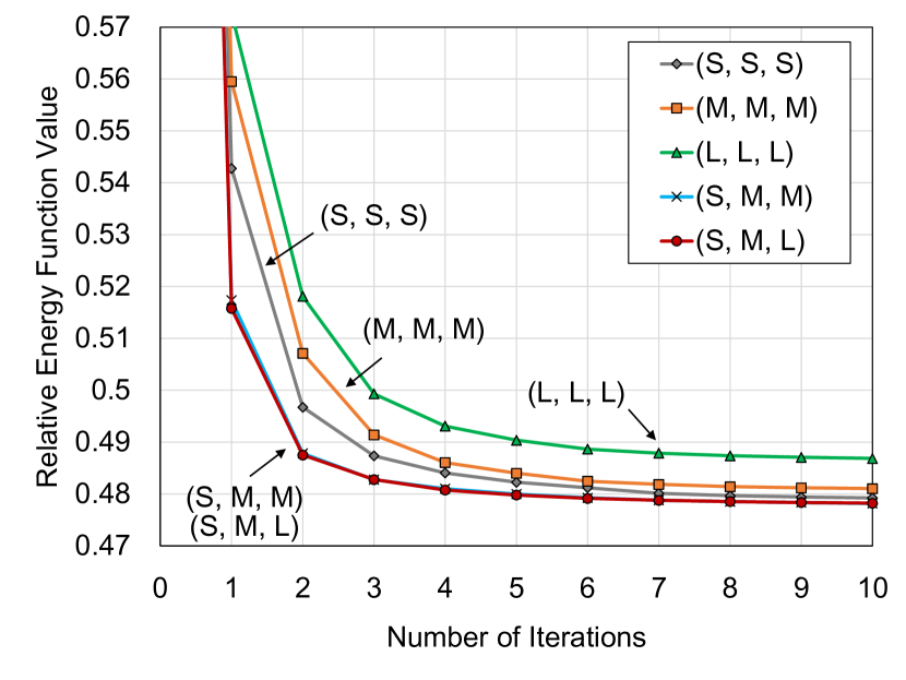
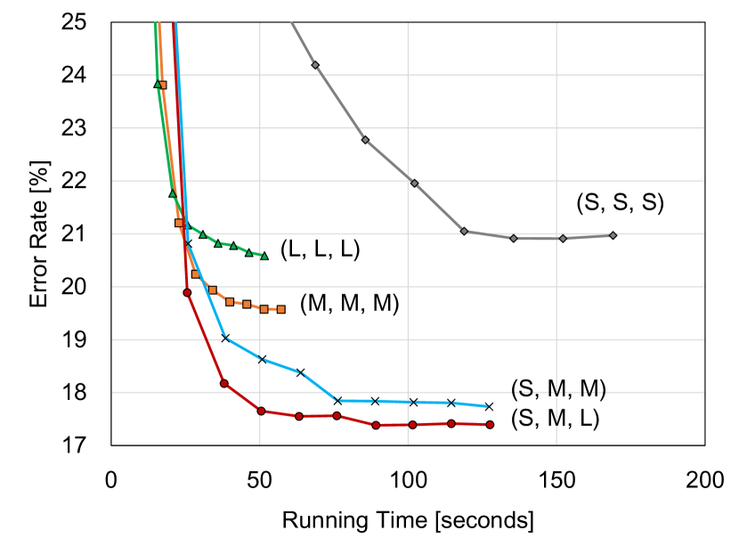
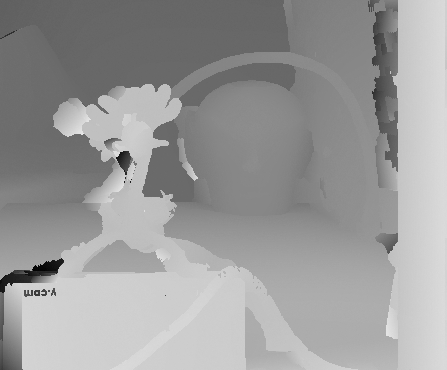
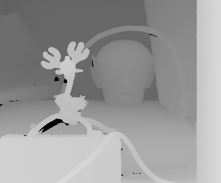
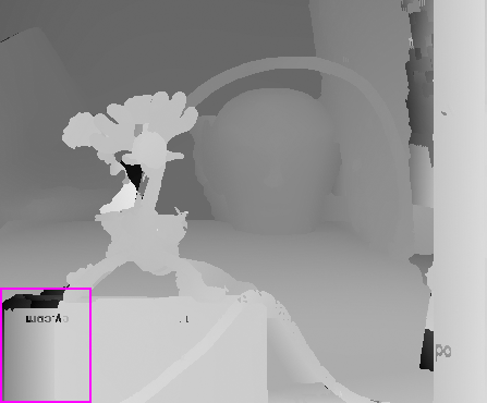
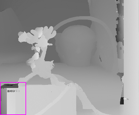
To observe the effect of grid-cell sizes, we use the three sizes of grid-cells, pixels (denoted as “S”mall), pixels (denoted as “M”edium), pixels (denoted as “L”arge), in different combinations and assess the performance using the following five different settings; (S, S, S): the small-size cells for all grid-structures; (M, M, M): the medium-size cells for all grid-structures; (L, L, L): the large-size cells for all grid-structures; (S, M, M): the small and medium-size cells for the first and the other two grid-structures, respectively; (S, M, L): the small, medium, and large-size cells for the first, second, and third grid-structures, respectively (the default setting for our method described above). Here, the iteration numbers for the first to third grid-structures are kept as default. We use the LE-GF method so as to access the effect on cost filtering acceleration as well. We use but keep the other parameters as default. Using these settings, we observe the performance variations by estimating the disparities of only the left image of the Reindeer dataset without post-processing.
The plots in Fig. 8 (a) show the transitions of the energy function values over iterations. The plots in Fig. 8 (b) show the temporal transitions of error rates with subpixel accuracy. As shown, the joint use of multiple cell sizes improves the performance in both energy reduction and accuracy. Although (S, M, M) and (S, M, L) show almost the same energy transitions, the proposed combination (S, M, L) shows faster and better convergence in accuracy.
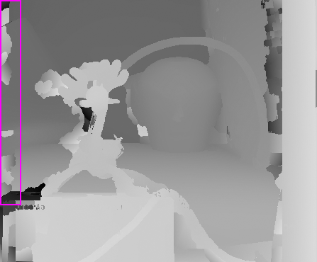
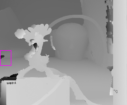
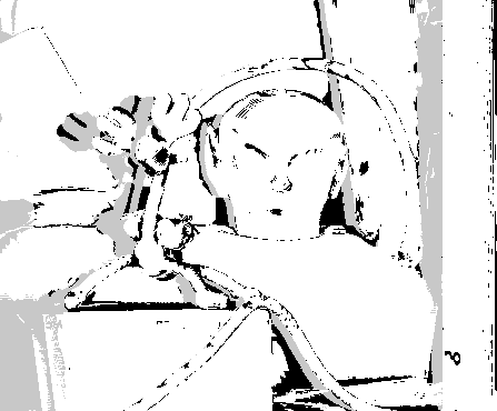
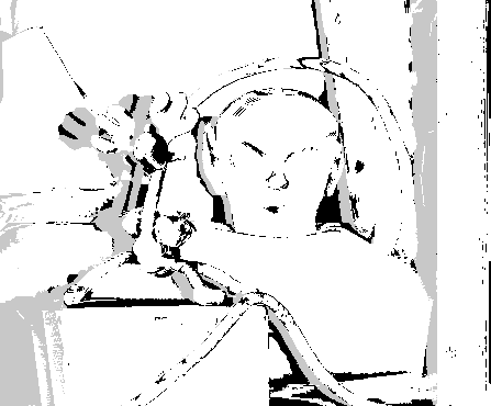
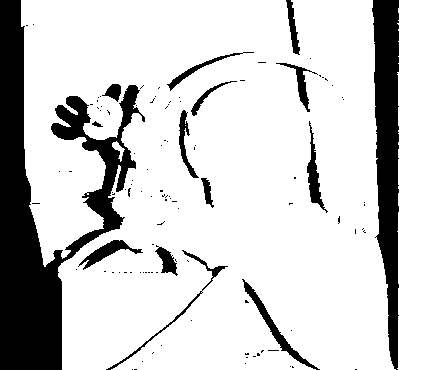
Figure 8 compares the results of the five settings with error maps for (S, M, M) and (S, M, L). The use of larger grid-cells helps to obtain smoother disparities, and it is especially effective for occluded regions.
Comparing the running times in Fig. 8 (b), the use of the small-size cells is inefficient due to the increased overhead in cost filtering, whereas the use of the medium and large-size cells achieves almost the same efficiency.
Effect of our post-processing (PP) and RANSAC proposer (RP). We show weighted average bad 2.0 scores of our LE-GF method with 3DMST [28] that ranks second following ours. We use 15 training image pairs from Middlebury V3. We also show average (avr) and standard deviation (stdev) by ten sets of different random initializations. See also Sec. 4.7 for more analysis on the RANSAC proposer.
| PP | RP | nonocc | all | |
| ✓ | ✓ | 6.52 | 12.1 | |
| Ours | ✓ | 6.65 | 13.6 | |
| 7.72 | 14.6 | |||
| avr stdev | ✓ | ✓ | 6.63 | 12.3 |
| 0.12 | 0.2 | |||
| ref. 3DMST [28] | ✓ | 7.08 | 12.9 |
(a) Energy function values w.r.t. iterations
(b) Temporal error-rate transitions

Reindeer
(S, S, S)
(S, M, M)
(S, M, L)
Ground truth
(M, M, M)
(L, L, L)
Error map of (S, M, M)
Error map of (S, M, L)
Visibility map
(a) Time-energy transitions (full)
(b) Time-energy transitions (zoomed)
(c) Error rate transitions
4.4 Efficiency evaluation in comparison to our previous algorithm [39]
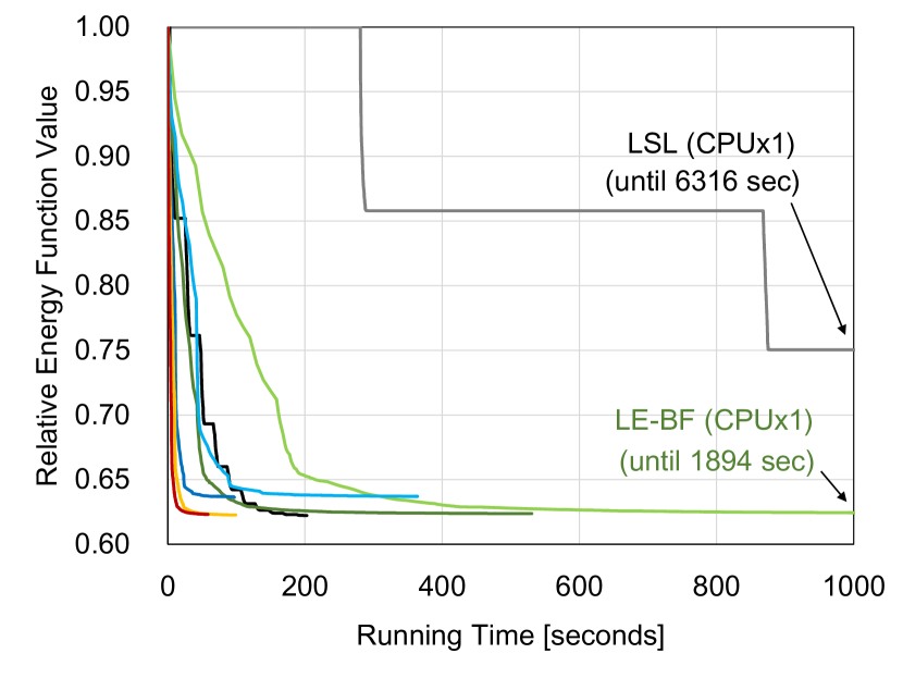
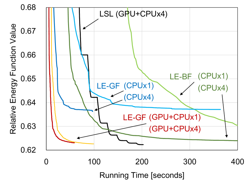
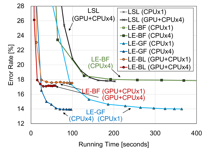
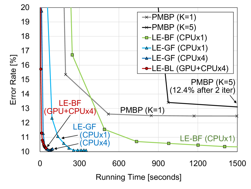
We evaluate the effectiveness of the three acceleration techniques: 1) parallelization of disjoint -expansions, and 2) acceleration of unary cost computation by GPU and 3) by cost filtering. For this, we compare following six variants of our method: LE-BF and LE-GF using one or four CPU cores (denoted as CPUx1 and CPUx4), and LE-BF using GPU and one or four CPU cores (denoted as GPU+CPUx1 and GPU+CPUx4). Additionally, we compare with our previous algorithm of [39] with CPU and GPU implementations (denoted as LSL with CPUx1 and GPU+CPUx4). We use the Rocks1 dataset by estimating the disparities of only the left image without post-processing. Figures 9 (a)–(c) show the temporal transitions of the energy values in the full and zoomed scales, and the subpixel error rates, respectively. Note that energy values in Fig. 9 are evaluated by the energy function of LE-BF and LSL for better visualization.
Parallelization of local -expansions on CPU: Comparing CPUx1 and CPUx4, we observe about 3.5x of speed-up for both LE-BF and LE-GF. Note that the converged energy values of LE-GF are relatively higher than the others because it optimizes a different energy function. However, if we see Fig. 9 (c), it actually finds better solutions in this example. On the other hand, speed-up for LE-BF from GPU+CPUx1 to GPU+CPUx4 is limited to about 1.7x. This is because the unary cost computation is already parallelized by GPU and this speed-up is accounted for by the parallelization of other parts, e.g., the computation of pairwise terms and min-cut.
Parallelization of unary cost computation on GPU: By comparing GPU+CPUx1 and CPUx1 of LE-BF, we obtain about 19x of speed-up. This is relatively smaller than 32x of speed-up in our previous LSL method, mainly due to the larger overhead of GPU data transferring.
Fast cost filtering: By comparing LE-GF and LE-BF methods, we observe about 5.3x speed-up for both CPUx1 and CPUx4 versions. Notably, even a CPU implementation of LE-GF (CPUx4) achieves almost comparable efficiency with a GPU implementation of LE-BF (GPU+CPUx1).
Comparison to our previous method [39]: In comparison to our previous LSL method [39], our LE-BF shows much faster convergence than LSL in the same single-core results (CPUx1). We consider there are mainly three factors contributing to this speed-up; First, the batch-cycle algorithm adopted in [39] makes its convergence slower; Second, we use cost filtering and compute its first step of Eq. (18) in , while [39] computes each unary term individually in ; Finally, we have removed a per-pixel label refinement step of [39] which requires additional unary-cost computations. Similar speed-up can be observed from LSL (GPU+CPUx4) to LE-BF (GPU+CPUx4).
4.5 Comparison with PMBP [3]
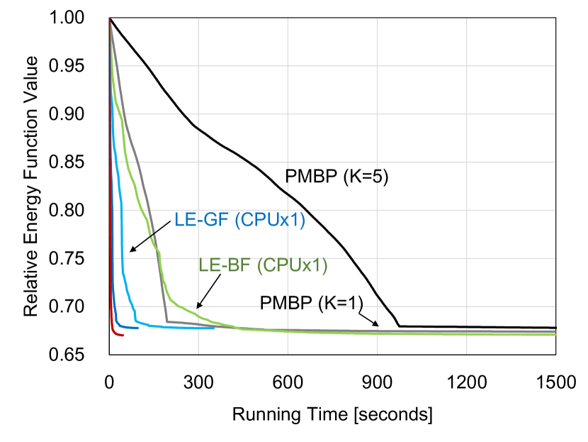
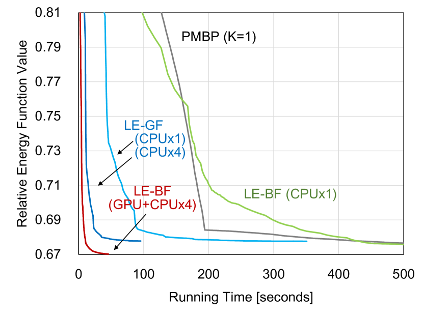
We compare our method with PMBP [3] that is the closest method to ours. For a fair comparison, we use four neighbors for in Eq. (5) as the same setting with PMBP. For a comparable smoothness weight with the default setting (eight-neighbor ), we use for LE-BF and for LE-GF, and keep the other parameters as default. For PMBP, we use the same model as ours; the only difference from the original PMBP is the smoothness term, which does not satisfy the submodularity of Eq. (2). In PMBP, it defines candidate labels for each pixel, for which we set and (original paper uses ). We show the comparison using the Cones dataset by estimating the disparities of only the left image without post-processing.
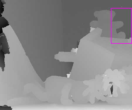
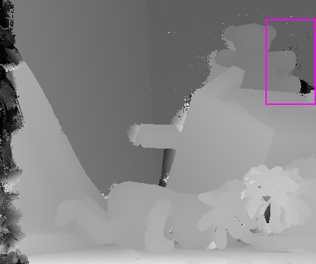
Figures 11 (a)–(c) show the temporal transitions of the energy values in the full and zoomed scales, and the subpixel error rates, respectively. We show the performance of our method using its GPU and CPU (one or four CPU cores) implementations. For PMBP, we also implemented the unary cost computation on GPU, but it became rather slow, due to the overhead of data transfer. Efficient GPU implementations for PMBP are not available in literature.555 GPU-parallelization schemes of BP are not directly applicable due to PMBP’s unique settings. The “jump flooding” used in the original PatchMatch [1] reports x speed-ups by GPU. However, because it propagates candidate labels to distant pixels, it is not applicable to PMBP that must propagate messages to neighbors, and is not as efficient as our x, either. Therefore, the plots show PMBP results that use a single CPU core. Figures 11 (a) and (b) show that, even with a single CPU-core implementation, our LE-BF and LE-GF show comparable or even faster convergence than PMBP. With CPU and GPU parallelization, our methods achieve much faster convergence than PMBP. Furthermore, our methods reach lower energies with greater accuracies than PMBP at the convergence. In Fig. 11 we compare the results of our LE-GF method and PMBP with . While PMBP yields noisy disparities, our method finds smoother and better disparities around edges and at occluded regions.
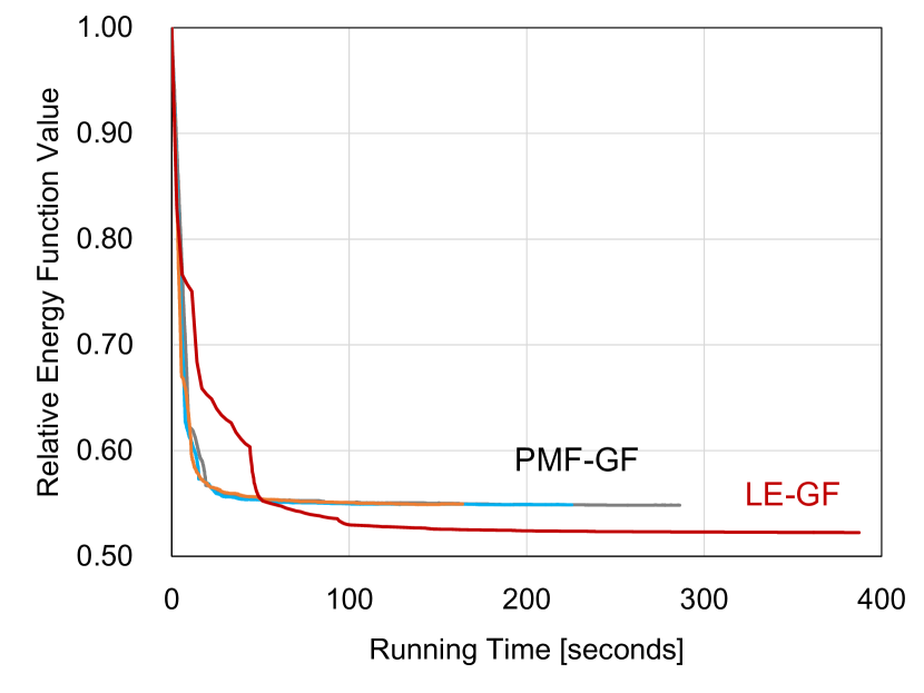
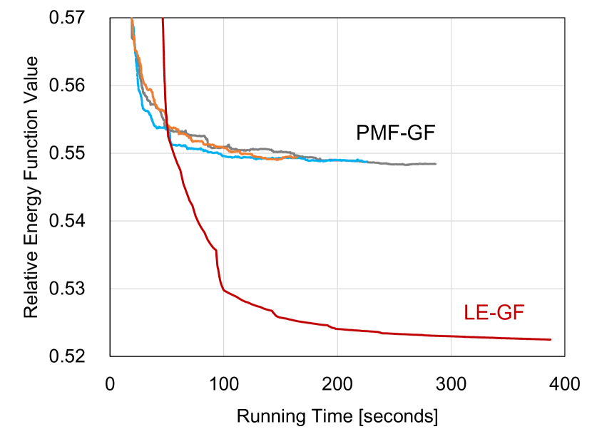
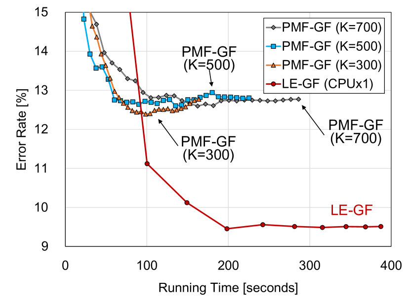
4.6 Comparison with PMF [32]
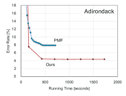
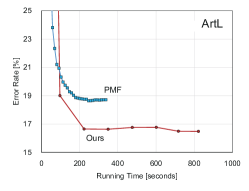
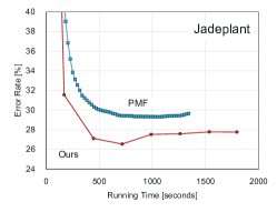
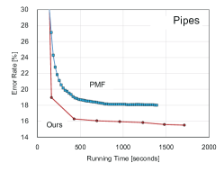
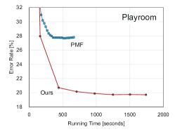
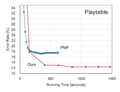
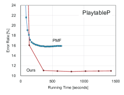
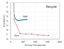
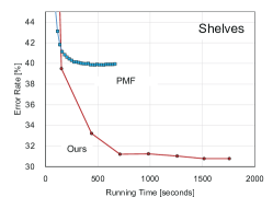
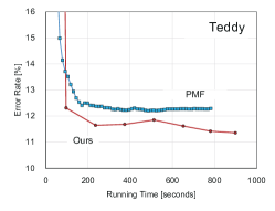
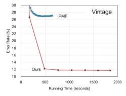
We also compare our LE-GF method with PMF [32] using the same data term as ours. For PMF, the number of superpixels is set to , , and as used in [32] ( is the default in [32]), and we sufficiently iterate 30 times. Both LE-GF and PMF are run using a single CPU core.
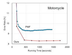
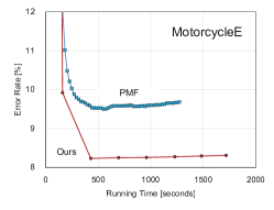
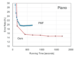
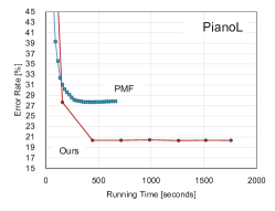
Figures 13 (a)–(c) show the temporal transitions of the energy values in the full and zoomed scales, and the subpixel error rates, respectively. As shown in Figs. 13 (a) and (b), PMF converges at higher energies than ours, since it cannot explicitly optimize pairwise smoothness terms because it is a local method. Furthermore, although energies are reduced almost monotonically in PMF, the transitions of accuracies are not stable and even degrade after many iterations. This is also because of the lack of explicit smoothness regularizer, and PMF converges at a bad local minimum. Figure 13 compares the results of our method and PMF with . Again, our methods find smoother and better disparities around edges and at occluded regions.
(a) Time-energy transitions (full)
(b) Time-energy transitions (zoomed)
(c) Error rate transitions
(a) Time-energy transitions (full)
(b) Time-energy transitions (zoomed)
(c) Error rate transitions
| Options | Teddy (from V2) | Adirondack | ArtL | Vintage | |||||||
| Reg. | Optimization | nonocc | all | disc | nonocc | all | nonocc | all | nonocc | all | |
| Ours (proposed LE-GF) | [33] | LE+RANSAC | 3.98 | 9.46 | 12.8 | 1.19 | 4.36 | 3.97 | 15.5 | 5.65 | 11.7 |
| Ours w/o RANSAC | [33] | LE | 4.26 | 9.19 | 13.6 | 1.20 | 4.63 | 3.98 | 15.3 | 13.7 | 18.7 |
| Ours w/o regularization | None | LE+RANSAC | 5.47 | 13.0 | 16.0 | 2.56 | 7.74 | 4.12 | 17.6 | 22.8 | 27.9 |
| Olsson et al. [33] + 3DPM | [33] | Fusion+RANSAC | 5.21 | 9.98 | 15.8 | 2.74 | 5.42 | 4.41 | 15.8 | 5.94 | 11.8 |
4.7 Comparison with Olsson et al. [33]
We compare with a stereo method by Olsson et al. [33], from which we borrow our smoothness term. As differences from our method, their data term does not use accurate slanted patch matching and they use conventional fusion-based optimization using planar proposals generated by RANSAC-based local plane fitting (see [33] for details). To compare optimization approaches of ours and [33], we replace the data term of [33] with ours so that the two methods use the same energy function as ours. We here use two variants of our LE-GF method that remove the RANSAC proposer and the regularization term, which are components closely related to [33]. We disable post-processing in all methods.
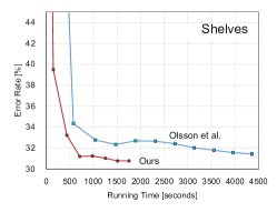
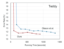
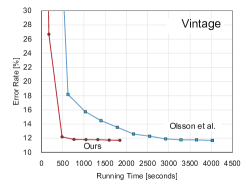
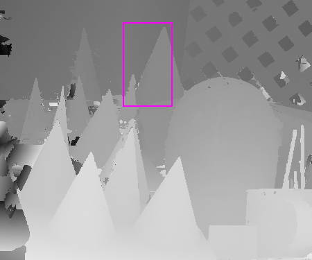
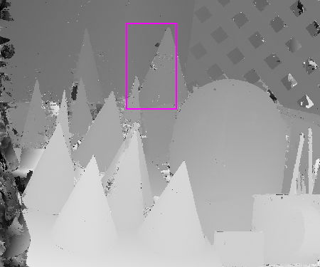
Table III shows error rates for Teddy from Middlebury V2 and three more datasets from V3, where the proposed method outperforms [33] and others. As shown in Figs. 16 and 16, our method has faster convergence and produces qualitatively better smooth surfaces than [33]. Spatial label propagation not only accelerates inference but also introduces an implicit smoothness effect [5], which helps our method to find smoother surfaces. Our method mostly performs comparably well regardless of the RANSAC proposer, outperforming [33]. On the other hand, the RANSAC proposer promotes convergence (see Fig. 16) and also effectively recovers large texture-less planes in Vintage (Fig. 16). Using a more advanced proposer [34] may lead to further improvements. Also note that, except for Vintage in Table III, our method performs well for non-occluded regions even without regularization (as comparable to [33]). The slanted patch matching term alone has an implicit second-order smoothness effect [5], and the regularizer of [33] further enforces it especially for occluded or texture-less regions.
5 Conclusions
In this paper, we have presented an accurate and efficient stereo matching method for continuous 3D plane label estimation. Unlike previous approaches that use fusion moves [25, 33, 45], our method is subproblem optimal and only requires a randomized initial solution. By comparing with a recent continuous MRF stereo method, PMBP [3], our method has shown an advantage in efficiency and comparable or greater accuracy. The use of a GC-based optimizer makes our method advantageous.
Acknowledgments
The authors would like to thank the anonymous reviewers including those of the conference paper. This work was supported by JSPS KAKENHI Grant Number 14J09001 and Microsoft Research Asia Ph.D. Fellowship.
References
- [1] C. Barnes, E. Shechtman, A. Finkelstein, and D. B. Goldman. PatchMatch: a randomized correspondence algorithm for structural image editing. Proc. of SIGGRAPH (ACM Trans. on Graph.), 28(3):24:1–24:11, 2009.
- [2] C. Barnes, E. Shechtman, D. B. Goldman, and A. Finkelstein. The generalized patchmatch correspondence algorithm. In Proc. of European Conf. on Computer Vision (ECCV), pages 29–43, 2010.
- [3] F. Besse, C. Rother, A. Fitzgibbon, and J. Kautz. PMBP: PatchMatch Belief Propagation for Correspondence Field Estimation. In Proc. of British Machine Vision Conf. (BMVC), pages 132.1–132.11, 2012.
- [4] S. Birchfield and C. Tomasi. Multiway cut for stereo and motion with slanted surfaces. In Proc. of Int’l Conf. on Computer Vision (ICCV), volume 1, pages 489–495, 1999.
- [5] M. Bleyer, C. Rhemann, and C. Rother. PatchMatch Stereo - Stereo Matching with Slanted Support Windows. In Proc. of British Machine Vision Conf. (BMVC), pages 14.1–14.11, 2011.
- [6] M. Bleyer, C. Rother, and P. Kohli. Surface stereo with soft segmentation. In Proc. of IEEE Conf. on Computer Vision and Pattern Recognition (CVPR), pages 1570–1577, 2010.
- [7] Y. Boykov and V. Kolmogorov. An experimental comparison of min-cut/max- flow algorithms for energy minimization in vision. IEEE Trans. Pattern Anal. Mach. Intell., 26(9):1124–1137, 2004.
- [8] Y. Boykov, O. Veksler, and R. Zabih. Fast approximate energy minimization via graph cuts. IEEE Trans. Pattern Anal. Mach. Intell., 23(11):1222–1239, 2001.
- [9] O. Chum, J. Matas, and J. Kittler. Locally Optimized RANSAC. In DAGM-Symposium, volume 2781, pages 236–243, 2003.
- [10] S. Drouyer, S. Beucher, M. Bilodeau, M. Moreaud, and L. Sorbier. Sparse Stereo Disparity Map Densification using Hierarchical Image Segmentation. In Proc. of Int’l Symp. on Mathematical Morphology, pages 172–184, 2017.
- [11] P. Felzenszwalb and D. Huttenlocher. Efficient belief propagation for early vision. In Proc. of IEEE Conf. on Computer Vision and Pattern Recognition (CVPR), volume 1, pages 261–268, 2004.
- [12] S. Geman and D. Geman. Stochastic Relaxation, Gibbs Distributions, and the Bayesian Restoration of Images. IEEE Trans. Pattern Anal. Mach. Intell., 6(6):721–741, 1984.
- [13] K. He, J. Sun, and X. Tang. Guided image filtering. IEEE Trans. Pattern Anal. Mach. Intell., 35(6):1397–1409, 2013.
- [14] P. Heise, S. Klose, B. Jensen, and A. Knoll. PM-Huber: PatchMatch with Huber Regularization for Stereo Matching. In Proc. of Int’l Conf. on Computer Vision (ICCV), pages 2360–2367, 2013.
- [15] L. Hong and G. Chen. Segment-based stereo matching using graph cuts. In Proc. of IEEE Conf. on Computer Vision and Pattern Recognition (CVPR), volume 1, pages 74–81, 2004.
- [16] A. Hosni, M. Gelautz, and M. Bleyer. Accuracy-Efficiency Evaluation of Adaptive Support Weight Techniques for Local Stereo Matching. In Proc. DAGM/OAGM Symposium, pages 337–346, 2012.
- [17] A. Hosni, C. Rhemann, M. Bleyer, C. Rother, and M. Gelautz. Fast cost-volume filtering for visual correspondence and beyond. IEEE Trans. Pattern Anal. Mach. Intell., 35(2):504–511, 2013.
- [18] J. Hur and S. Roth. MirrorFlow: Exploiting Symmetries in Joint Optical Flow and Occlusion Estimation. In Proc. of Int’l Conf. on Computer Vision (ICCV), 2017. (to appear).
- [19] H. Ishikawa. Exact optimization for Markov random fields with convex priors. IEEE Trans. Pattern Anal. Mach. Intell., 25(10):1333–1336, 2003.
- [20] K. R. Kim and C. S. Kim. Adaptive smoothness constraints for efficient stereo matching using texture and edge information. In Proc. of Int’l Conf. on Image Processing (ICIP), pages 3429–3433, 2016.
- [21] V. Kolmogorov. Convergent Tree-Reweighted Message Passing for Energy Minimization. IEEE Trans. Pattern Anal. Mach. Intell., 28(10):1568–1583, 2006.
- [22] V. Kolmogorov and C. Rother. Minimizing Nonsubmodular Functions with Graph Cuts – A Review. IEEE Trans. Pattern Anal. Mach. Intell., 29(7):1274–1279, 2007.
- [23] V. Kolmogorov and R. Zabih. Computing visual correspondence with occlusions using graph cuts. In Proc. of Int’l Conf. on Computer Vision (ICCV), volume 2, pages 508–515, 2001.
- [24] V. Kolmogorov and R. Zabin. What energy functions can be minimized via graph cuts? IEEE Trans. Pattern Anal. Mach. Intell., 26(2):147–159, 2004.
- [25] V. Lempitsky, C. Rother, S. Roth, and A. Blake. Fusion Moves for Markov Random Field Optimization. IEEE Trans. Pattern Anal. Mach. Intell., 32(8):1392–1405, 2010.
- [26] A. Li, D. Chen, Y. Liu, and Z. Yuan. Coordinating multiple disparity proposals for stereo computation. In Proc. of IEEE Conf. on Computer Vision and Pattern Recognition (CVPR), pages 4022–4030, 2016.
- [27] G. Li and S. W. Zucker. Differential geometric inference in surface stereo. IEEE Trans. Pattern Anal. Mach. Intell., 32(1):72–86, 2010.
- [28] L. Li, X. Yu, S. Zhang, X. Zhao, and L. Zhang. 3d cost aggregation with multiple minimum spanning trees for stereo matching. Appl. Opt., 56(12):3411–3420, 2017.
- [29] L. Li, S. Zhang, X. Yu, and L. Zhang. PMSC: PatchMatch-Based Superpixel Cut for Accurate Stereo Matching. IEEE Transactions on Circuits and Systems for Video Technology, PP(99):1–1, 2017.
- [30] J. Liu and J. Sun. Parallel graph-cuts by adaptive bottom-up merging. In Proc. of IEEE Conf. on Computer Vision and Pattern Recognition (CVPR), pages 2181–2188, 2010.
- [31] J. Lu, K. Shi, D. Min, L. Lin, and M. Do. Cross-based local multipoint filtering. In Proc. of IEEE Conf. on Computer Vision and Pattern Recognition (CVPR), pages 430–437, 2012.
- [32] J. Lu, H. Yang, D. Min, and M. N. Do. Patch Match Filter: Efficient Edge-Aware Filtering Meets Randomized Search for Fast Correspondence Field Estimation. In Proc. of IEEE Conf. on Computer Vision and Pattern Recognition (CVPR), pages 1854–1861, 2013.
- [33] C. Olsson, J. Ulen, and Y. Boykov. In Defense of 3D-Label Stereo. In Proc. of IEEE Conf. on Computer Vision and Pattern Recognition (CVPR), pages 1730–1737, 2013.
- [34] C. Olsson, J. Ulén, and A. Eriksson. Local Refinement for Stereo Regularization. In Proc. of Int’l Conf. on Pattern Recognition (ICPR), pages 4056–4061, 2014.
- [35] G. Petschnigg, R. Szeliski, M. Agrawala, M. Cohen, H. Hoppe, and K. Toyama. Digital photography with flash and no-flash image pairs. ACM Trans. on Graph., 23(3):664–672, 2004.
- [36] C. Rhemann, A. Hosni, M. Bleyer, C. Rother, and M. Gelautz. Fast cost-volume filtering for visual correspondence and beyond. In Proc. of IEEE Conf. on Computer Vision and Pattern Recognition (CVPR), pages 3017–3024, 2011.
- [37] P. Strandmark and F. Kahl. Parallel and distributed graph cuts by dual decomposition. In Proc. of IEEE Conf. on Computer Vision and Pattern Recognition (CVPR), pages 2085–2092, 2010.
- [38] R. Szeliski, R. Zabih, D. Scharstein, O. Veksler, V. Kolmogorov, A. Agarwala, M. Tappen, and C. Rother. A Comparative Study of Energy Minimization Methods for Markov Random Fields with Smoothness-Based Priors. IEEE Trans. Pattern Anal. Mach. Intell., 30(6):1068–1080, 2008.
- [39] T. Taniai, Y. Matsushita, and T. Naemura. Graph Cut based Continuous Stereo Matching using Locally Shared Labels. In Proc. of IEEE Conf. on Computer Vision and Pattern Recognition (CVPR), pages 1613–1620, 2014.
- [40] T. Taniai, S. N. Sinha, and Y. Sato. Joint Recovery of Dense Correspondence and Cosegmentation in Two Images. In Proc. of IEEE Conf. on Computer Vision and Pattern Recognition (CVPR), pages 4246–4255, 2016.
- [41] H. Tao, H. Sawhney, and R. Kumar. A global matching framework for stereo computation. In Proc. of Int’l Conf. on Computer Vision (ICCV), volume 1, pages 532–539, 2001.
- [42] L. Wang and R. Yang. Global stereo matching leveraged by sparse ground control points. In Proc. of IEEE Conf. on Computer Vision and Pattern Recognition (CVPR), pages 3033–3040, 2011.
- [43] Z.-F. Wang and Z.-G. Zheng. A region based stereo matching algorithm using cooperative optimization. In Proc. of IEEE Conf. on Computer Vision and Pattern Recognition (CVPR), 2008.
- [44] Y. Wei and L. Quan. Asymmetrical Occlusion Handling Using Graph Cut for Multi-View Stereo. In Proc. of IEEE Conf. on Computer Vision and Pattern Recognition (CVPR), pages 902–909, 2005.
- [45] O. Woodford, P. Torr, I. Reid, and A. Fitzgibbon. Global Stereo Reconstruction under Second-Order Smoothness Priors. IEEE Trans. Pattern Anal. Mach. Intell., 31(12):2115–2128, 2009.
- [46] K. Yamaguchi, T. Hazan, D. McAllester, and R. Urtasun. Continuous markov random fields for robust stereo estimation. In Proc. of European Conf. on Computer Vision (ECCV), pages 45–58, 2012.
- [47] J. S. Yedidia, W. T. Freeman, and Y. Weiss. Generalized Belief Propagation. In Advances in Neural Information Processing Systems (NIPS), volume 13, pages 689–695, 2000.
- [48] K.-J. Yoon and I.-S. Kweon. Locally adaptive support-weight approach for visual correspondence search. In Proc. of IEEE Conf. on Computer Vision and Pattern Recognition (CVPR), volume 2, pages 924–931, 2005.
- [49] J. Zbontar and Y. LeCun. Stereo matching by training a convolutional neural network to compare image patches. Journal of Machine Learning Research, 17:1–32, 2016.
Supplementary Material for
Continuous 3D Label Stereo Matching using
Local Expansion Moves
Appendix A Proof of Lemma 1
Proof.
For the completeness, we repeat the original proof given in [33] with our notations. Regarding ,
Thus, satisfies the submodularity of expansion moves. For its truncated function,
Therefore, also satisfies the submodularity. ∎
Appendix B Additional results
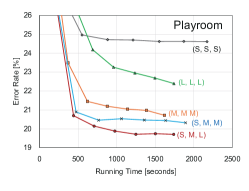
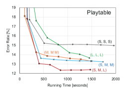
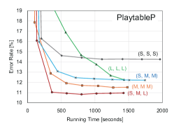
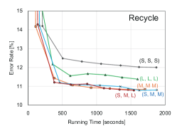
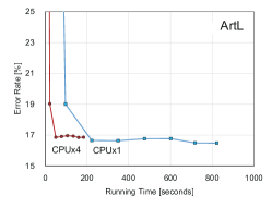
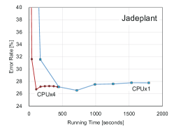
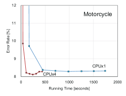
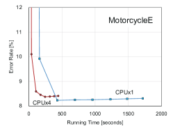
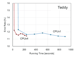
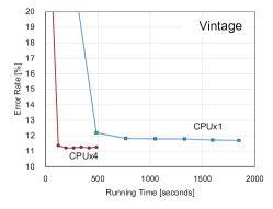
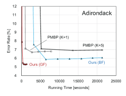
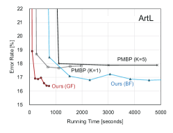
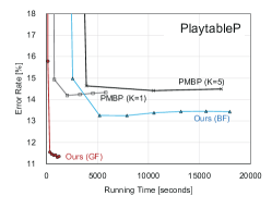
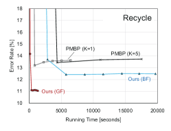
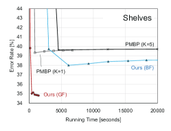
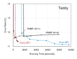
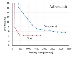
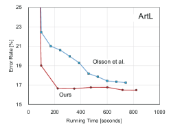
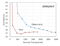
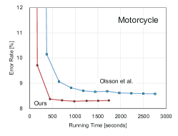
We here provide additional results for the analyses on effects of grid-cell sizes (Sec. 4.3) and parallelization (Sec. 4.4) as well as the comparisons with the methods of PMBP [3] (Sec. 4.5), PMF [32] (Sec. 4.6) and Olsson et al. [33] (Sec. 4.7). We evaluate performances by showing plots of error rate transitions over running time, where error rates are evaluated by the bad 2.0 metric for all regions. To provide diverse examples, we use 15 image pairs from the Middlebury V3 training dataset.
Unless noted otherwise, all methods are run on a single CPU core to optimize the same energy function that we use in Sec. 4.2 for the benchmark V3 evaluation. Settings of our method are also the same as we use in Sec. 4.2. Post-processing is disabled in all methods.
Effect of grid-cell sizes
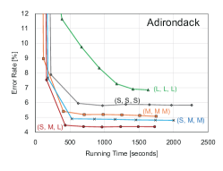
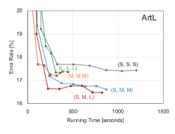
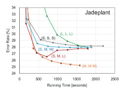
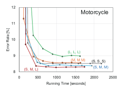
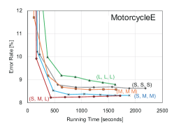
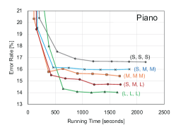
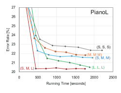
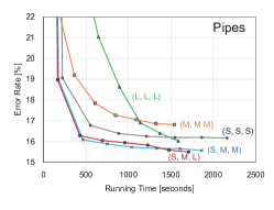
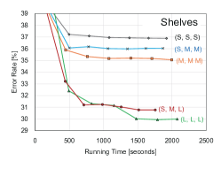
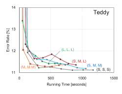
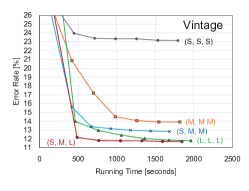
Figure A1 shows analyses on effects of grid-cell sizes. Similarly to Sec. 4.3, we compare the proposed grid-cell combination (S, M, L) with other four combinations (L, L, L), (M, M, M), (S, S, S), and (S, M, M). Here, the sizes of “S”mall, “M”edium, and “L”arge grid-cells are proportionally set to , and of the image width, respectively. For most of the image pairs, the proposed combination (S, M, L) performs best among the five combinations.
Efficiency comparison by parallelization
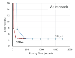
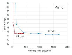
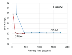
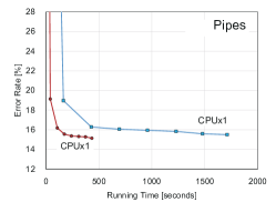
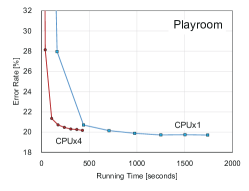
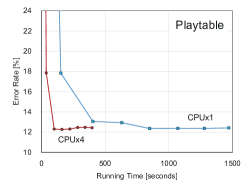
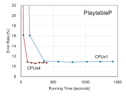
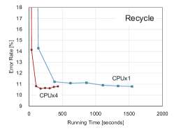
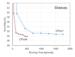
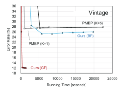
Figure A2 shows analyses on parallelization of our local expansion move algorithm. When our method is performed in parallel on four CPU cores, we observe about 3.8x of average speed-up among the 15 image pairs.
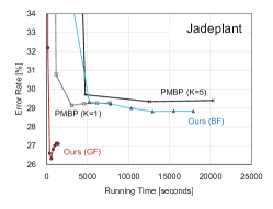
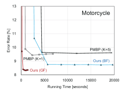
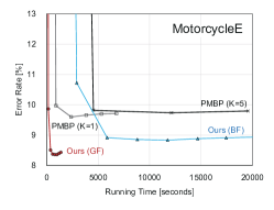
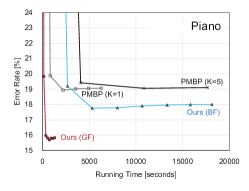
Comparison with PMBP [3]
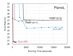
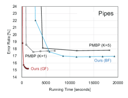
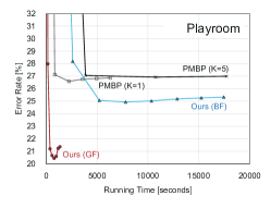
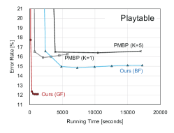
Figure A3 compares our method with PMBP [3]. Similarly to Sec. 4.4, we compare PMBP (using and ) with two variants of our method using guided image filtering (GF) and bilateral filtering (BF). Because PMBP cannot use the cost-map filtering acceleration of GF, we use only BF for PMBP. Therefore, our method using BF optimizes the same energy function with PMBP, while ours using GF optimizes a different function. All methods use four neighbors of pairwise terms as the same setting with PMBP.
Comparison with PMF [32]
Comparison with Olsson et al. [33]
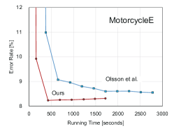
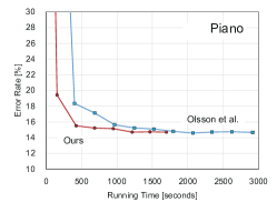
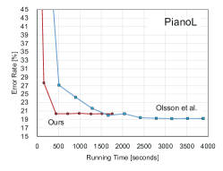
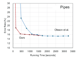
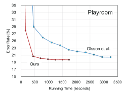
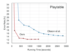
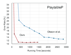
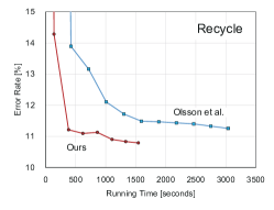
Figure A5 compares our method with the method by Olsson et al. [33]. Both methods use the same energy function but optimize it differently. For most of the image pairs, our method is about 6x faster to reach comparable or better accuracies than [33]. Our method can be further accelerated by parallelization as demonstrated in Fig. A2.




![[Uncaptioned image]](/html/1603.08328/assets/x26.png)
![[Uncaptioned image]](/html/1603.08328/assets/figure/comp_olsson/art_3d/ours.png)
![[Uncaptioned image]](/html/1603.08328/assets/figure/comp_olsson/art_3d/olsson.png)
![[Uncaptioned image]](/html/1603.08328/assets/figure/comp_olsson/Vintage/im0.png)
![[Uncaptioned image]](/html/1603.08328/assets/figure/comp_olsson/Vintage/ours.png)
![[Uncaptioned image]](/html/1603.08328/assets/figure/comp_olsson/Vintage/ours_noransac.png)
![[Uncaptioned image]](/html/1603.08328/assets/figure/comp_olsson/Vintage/olsson.png)