Image Super-Resolution Based on Sparsity Prior via Smoothed $l_{0}$ Norm

Abstract

In this paper we aim to tackle the problem of reconstructing a high-resolution image from a single low-resolution input image, known as single image super-resolution. In the literature, sparse representation has been used to address this problem, where it is assumed that both low-resolution and high-resolution images share the same sparse representation over a pair of coupled jointly trained dictionaries. This assumption enables us to use the compressed sensing theory to find the jointly sparse representation via the low-resolution image and then use it to recover the high-resolution image. However, sparse representation of a signal over a known dictionary is an ill-posed, combinatorial optimization problem. Here we propose an algorithm that adopts the smoothed $l_{0}$-norm (SL0) approach to find the jointly sparse representation. Improved quality of the reconstructed image is obtained for most images in terms of both peak signal-to-noise-ratio (PSNR) and structural similarity (SSIM) measures.

I INTRODUCTION

Image super-resolution provides a low cost, software-based technique to improve the spatial resolution of an image beyond the limitations of the imaging hardware devices. The areas of application include medical imaging [1] and satellite imaging [2] and high-definition television (HDTV). In such cases, it is standard to assume that the observed low-resolution image(s) is a blurred and downsampled version of the high-resolution image. The goal is then to recover the high-resolution image using its low-resolution observation(s). Meanwhile, with the growing capabilities of high-resolution displays, effective image super-resolution algorithms is essential for us to make the best use of such devices.

The most typical super-resolution methods require multiple low-resolution images, with sub-pixel accuracy alignment. In this approach super-resolution can be considered as an inverse problem, where it is essential to assume a prior on the solution to regularize the ill-posed nature of the problem and avoid infinitely many solutions [3, 4].

In some applications, the number of low-resolution images is limited and it is desired to reconstruct the high resolution image from a single low-resolution image. One approach to overcome this limitation is to use interpolation methods [5, 6, 7], where unknown pixels of the high-resolution image are estimated using nearby known pixels from the low-resolution image based on some assumptions on the relation between pixels. Simple interpolation methods such as bilinear and bicubic interpolations result in blued images with ringing artifacts near edges. While more advanced methods [6, 7] try to avoid this problem by exploiting natural image priors, they are often limited in accounting for the complexity of images which have regions with fine textures or smooth shadings. As a result, watercolor-like artifacts are often observed in some regions.

A more successful class of methods for single input image super-resolution are learning based methods. Here a co-occurrence prior between the high-resolution and low-resolution images is used to reconstruct the high-resolution image [8, 9, 10, 11]. The learning procedure has been done via different schemes such as Markov Random Field (MRF), Primal Sketch and Locally Linear Embedding (LLE) [8, 9, 10]. These algorithms require enormous databases to handle the learning stage and thus are computationally expensive. One of the recently developed successful methods [11] uses sparsity as the co-occurrence prior between the high-resolution and low-resolution images. This approach reduces the size of the training database and consequently the computational load. In this method it is assumed that both images share the same sparse representation over a pair of jointly trained dictionaries. Using this assumption we can find the jointly sparse representation via the low-resolution image and then use it to recover the high-resolution image. Finding the jointly sparse representation properly, is important and influences the quality of the reconstruction result. In the current paper our intention is to improve the performance of this algorithm to find the jointly sparse representation more accurately and thus to improve the quality of the reconstructed high-resolution image.

Sparse representation of a vector over a known dictionary is an ill-posed, combinatorial optimization problem [12]. Several relaxation approaches have been used to convexify this problem. The most common approaches are Matching Pursuit (MP)[13], Basis Pursuit (BP) [14], and Focal Underdetermined System Solution (FOCUSS) [15]. In this paper, we adopt a recently proposed Smoothed $l_{0}$-norm (SL)) algorithm [16], a faster solver for sparse representation, to lessen the computational load and to improve the quality of the reconstructed high-resolution image.

The rest of the paper is organized as follows. In section II, we briefly present the approach that is used to decompose a signal on an overcomplete dictionary. Section III is devoted to the super-resolution algorithm and its alternation. Section VI summarizes experimental results. The paper is finally concluded in section V.

II SPARSE REPRESENTATION VIA SMOOTHED $l_{0}$ NORM

Finding the sparsest representation of a source signal over an overcomplete dictionary is formulated under the topic of compressed sensing (CS) theory [12, 17]. Let ${\bf x}\in\mathbb{R}^{n}$ be the source signal, and $D\in\mathbb{R}^{m\times n}$ the dictionary ($n>m$). Our goal is to find the sparsest solution of the following linear system:

$${\bf x}=D\alpha,$$ (1)

where $\alpha\in\mathbb{(}R)^{m}$. The recovery of $\alpha$ from ${\bf x}$ based on (1) is impossible to implement in a unique and stable way, unless it is known that $\alpha$ is sparse enough to have a relatively low value of $\|\alpha\|_{0}$ [12]. This assumption is only valid if the dictionary is chosen or learned properly. Several algorithms have been provided to design such dictionaries [18, 19, 20].

Equivalently (1) can be formulated as the following optimization problem:

$$(P_{0})\hskip 14.22636pt\min\|\alpha\|_{0},\hskip 8.53581pt\text{s.t.}\hskip 8.53581pt{\bf x}=D\alpha$$ (2)

Due to the highly nonconvex nature of $l_{0}$-norm, this problem is ill-posed and intractable. In conventional CS theory [12, 17] it is proven that if the dictionary $D$ satisfies the restricted isometry property (RIP) [12, 17] with respect to a certain class of sparse signals to which $\alpha$ is assumed to belong, then $\alpha$ can be recovered as a solution to [21, 22]

$$(P_{1})\hskip 14.22636pt\min\|\alpha\|_{1},\hskip 8.53581pt\text{s.t.}\hskip 8.53581pt{\bf x}=D\alpha$$ (3)

which is a convex minimization problem. It is straightforward to reformulate this equivalent problem in terms of linear programming. This approach results in a tractable problem but is still time-consuming for large scale systems. It is also important to note that the equivalence between $l_{0}$-norm and $l_{1}$-norm is only valid asymptotically and does not always hold [23]. In a different approach, the $l_{0}$-norm is approximated directly by a smooth convex function [16]. This approach has proved to be faster with possibility of resulting in sparser representation [16].

Consider the smooth function, $f_{\sigma}(x)=e^{-x^{2}/\sigma^{2}}$. As $\sigma$ approaches zero, we have the following equivalence:

$$\|{\bf x}\|_{0}=n-\sum_{i=0}^{n}\lim_{\sigma\to 0^{+}}f_{\sigma}(x_{i})=n-\sum_{i=0}^{n}f_{0^{+}}(x_{i})$$ (4)

This equivalence does not help us in practice. However, one can assume that if $\sigma$ is set to be nonzero and sufficiently small then we can approximate the $l_{0}$-norm of a vector by

$$\|{\bf x}\|_{0}\approx n-\sum_{i=0}^{n}f_{\sigma}(x_{i})$$ (5)

This enables us to approximate the $l_{0}$-norm with a smooth, differentiable function. This is the key fact that enables us to replace the $l_{0}$-norm minimization with a convex problem, so that we can take advantage of common techniques, such as steepest descent, to tackle the optimization problem. The value of $\sigma$ controls the trade-off between the closeness to the $l_{0}$-norm and the smoothness of the approximation. Now if we define $F_{\sigma}({\bf x})=\sum_{i=0}^{n}f_{\sigma}(x_{i})$, then the minimization of $\|{\bf x}\|_{0}$ can be done by maximizing $F_{\sigma}$ by choosing a proper value for $\sigma$. Due to the nonconvex nature of the $l_{0}$-norm, $F_{\sigma}$ will archive a lot of local extreme points for small values of $\sigma$. Consequently, finding the global maxima will become difficult. On the other hand, if the value of $\sigma$ is chosen to be sufficiently large, there will be no local maxima [16] and asymptotically the solution for $\sigma=\infty$ is equivalent to the $l_{2}$-norm solution. Considering these facts, the authors of [16] provided Algorithm 1 to solve the optimization problem $P_{0}$.

1. Initialization:

a. Choose an arbitrary solution from the feasible set, e.g., the minimum $l_{2}$-norm solution of $D\alpha={\bf x}$, i.e., $\alpha=D^{T}(DD^{T})^{-1}{\bf x}$.

b. Choose a decreasing sequence for $\sigma$, $[\sigma_{1},...,\sigma_{K}]$.

for $k=1,...,K$:

a. Let $\sigma=\sigma_{k}$.

b. Maximize the function $F_{\sigma}$ using $L$ iterations of the steepest ascent algorithm and call it $v_{k}$.

Final answer is $\alpha=v_{K}$.

Algorithm 1 Sparse Representation using smoothed $l_{0}$-norm

Here, the final estimation of each step is used for the initialization of the next steepest ascent. By a proper selection of the sequence of $\sigma$, we may avoid being trapped in the local maxima. Compared to conventional CS solvers, this algorithms proves to be faster with the possibility of recovering a sparser solution [16].

III IMAGE SUPER-RESOLUTION BASED ON SPARSE REPRESENTATION

Sparse representation has been applied to multiple inverse problems in image processing such as denoising [24], restoration [25] and super-resolution [11, 4]. Generally sparsity is used as a prior on source signal to avoid ill-posed nature of inverse problems. In such applications, there exist a stage, which involves expansion of a source signal over an overcomplete dictionary, sparsely. The output quality of these algorithms depends on the accuracy in finding the sparse representation. In this section, SL0 algorithm is employed in a super-resolution algorithm to improve quality of the output high-resolution image.

Assume that the low-resolution image $\mathbf{Y}$ is produced from a high resolution image $\mathbf{X}$ by

$$\mathbf{Y}=SH\mathbf{X}$$ (6)

where $H$ represents a blurring matrix, and $S$ is a downsampling matrix. The recovered high-resolution output image must be consistent with the low-resolution input image. This problem is highly ill-posed and infinitely many solutions satisfy (6) and are consistent with low-resolution image. To provide a unique solution, local sparsity model maybe applied as a prior. We assume that there exist two dictionaries, $D_{l}$ and $D_{h}$, for which each patch of low, $y$, and high, $x$, resolution images can be represented sparsely simultaneously and jointly as follows:

$$\begin{split}x=D_{h}\alpha\\ y=D_{l}\alpha\end{split}$$ (7)

These coupled dictionaries are trained simultaneously and jointly over a set of low/high resolution images such that both low/high resolution images result in the same sparse representation coefficients. Having the dictionaries trained, for each patch of our low resolution image we need to calculate the sparse representation. The authors of [11] used $l_{1}$-norm minimization method for this propose. Here Algorithm 1 is adopted. Having the sparse representation, calculated using the low-resolution patch, we reconstruct the high resolution image patches using the high resolution dictionary, $D_{h}$. The patches are chosen to overlap so as to reduce the artifacts in patch boundaries. Next we regularize and merge the patches to produce an entire image using the reconstruction constraint (6). These procedure can be formulated as the following optimization problems:

$$\bm{\hat{\alpha}}_{ij}=\underset{\bm{\alpha}}{\operatorname{argmin}}\;\mu_{ij}||\bm{\alpha}||_{0}+||D_{l}\bm{\alpha}-\mathbf{R}_{ij}\mathbf{Y}||^{2}_{2},$$ (8)

$$\hat{\mathbf{X}}=\underset{\mathbf{X}}{\operatorname{argmin}}\;\;||\mathbf{X}-\mathbf{X}_{0}||^{2}_{2}+\lambda||SH\mathbf{X}-\mathbf{Y}||^{2}_{2},$$ (9)

where $\mathbf{R}_{ij}$ is a matrix that extracts the ($ij$) block from the image, $D_{l}\in\mathbb{R}^{m\times n}$ is the dictionary with $n>m$, $\lambda$ is the regularization parameter, $\mathbf{X}_{0}$ is the image obtained by averaging the blocks obtained using sparse representation, and $\bm{\alpha}_{ij}$ is the sparse vector of coefficients corresponding to the ($ij$) block of the image. Here, (8) refers to the sparse coding of local image patches with bounded prior, hence building a local model from sparse representations. On the other hand, (9) demands the proximity between the low-resolution image, $\mathbf{Y}$, and the output image $\mathbf{X}$, thus enforcing the global reconstruction constraint. In [11], $l_{1}$-norm minimization is used to solve (8) , whereas we use SL0 algorithm to solve this stage. The solution to (9) can be done iteratively using a gradient descent algorithm as follows:

$$\begin{split}\mathbf{X}_{t+1}=\mathbf{X}_{t}+\nu[H^{T}S^{T}(\mathbf{Y})-SH\mathbf{X}_{t}+\lambda(\mathbf{X}-\mathbf{X}_{0})]\end{split}$$ (10)

where $\mathbf{X}_{t}$ is the estimation of the high-resolution image after the $t$-th iteration, and $\nu$ is the step size.

The proposed image super-resolution algorithm is summarized in Algorithm 2.

1. Dictionary Training Phase: train high/low resolution dictionaries $D_{l}$, $D_{h}$, [11]

Reconstruction Phase

• Sparse coding stage: use Algorithm 1 to compute

the representation vectors $\alpha_{ij}$ for all the patches of low resolution image

High resolution patches reconstruction: using the found coefficients, $\alpha_{ij}$, the high resolution patches are reconstructed by multiplying them by$D_{h}$

Global Reconstruction: merge high-resolution patches by averaging over the overlapped region and then use (10) to result the high resolution image.

Algorithm 2 Image super resolution based on sparsity prior via smoothed $l_{0}$-norm

Compared to the original algorithm in [11], reduction in the computational complexity and the possibility of improving the output quality are expected.

IV EXPERIMENTAL RESULTS

In this section we compare the proposed super-resolution algorithm with bicubic interpolation and the method given in [11]. The image super resolution methods are tested on various images. To be consistent with [11], patches of $5\times 5$ pixels were used on the low resolution image and the scaling factor was set to $2$. Each patch is converted to a vector with length $25$. The trained dictionaries, provided by authors of [11], with the sizes of $25\times 1024$ and $100\times 1024$ for the low and the high resolution dictionaries were used, respectively. To remove artifacts on the patch boundaries we set a overlap of one pixel in the patches.

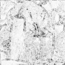
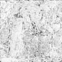
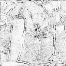
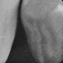
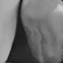
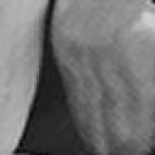
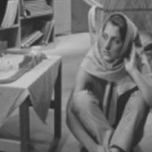
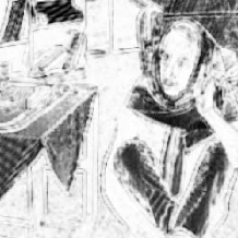
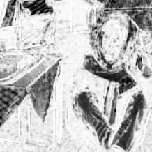
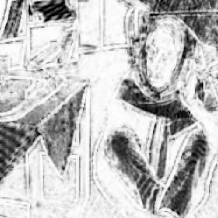
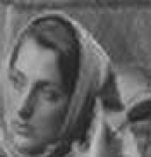
Fig. 1 and Fig. 2 (subplots (a) and (e)) depict the original Pepper and Barbara images and their corresponding low-resolution versions. In the same figures subplots (b-d) depict reconstructed high-resolution images using the proposed methods. Subplots (f-h) depict the corresponding SSIM maps [26]. A close look on the reconstructed images, enlarged image regions (subplots (i-l)), and the corresponding SSIM maps shows that while bicubic method works pretty well in smooth regions, significant blurring occurs on edges. The method of [11] is able to recover the edges better but does not work as well in smooth regions. Compared to [11] our approach is able to recover the edges and meanwhile it works better in smooth regions. One possible approach for further improving the image quality might be using a combination of bicubic and our approach. The quantitative results for different images reconstructed from different algorithms are shown in Table 1.

Figure 1: Original Pepper image (subplot (a)), its low-resolution version (subplot (e)), high-resolution images reconstructed by (subplot (b)) Bicubic, (subplot (c)) Yang et. al., (subplot (d)) proposed method, the corresponding SSIM maps (subplots (f-h)), and enlarged region (subplots (i-l))..

TABLE I: SSIM and PSNR comparisons of image super resolution results

Image	Barbara	Lena	Baboon	House	Watch	Pepper	Parthenon	Splash	Aeroplane	Tree	Girl	Bird	Average
	PSNR comparison (in dB)
Bicubic	27.08	32.70	26.34	33.97	26.94	30.84	28.07	33.58	28.50	29.41	35.12	29.49	30.17
Yang et al.	27.15	33.33	26.41	34.00	27.32	30.41	28.41	33.87	29.02	29.60	34.52	29.63	30.31
Proposed	27.13	33.45	26.52	33.97	27.41	30.55	28.68	34.13	29.24	29.67	35.25	29.82	30.49
	SSIM comparison
Bicubic	0.744	0.876	0.700	0.870	0.790	0.869	0.763	0.871	0.857	0.852	0.925	0.877	0.832
Yang et al.	0.747	0.884	0.702	0.873	0.806	0.850	0.765	0.918	0.868	0.857	0.901	0.882	0.837
Proposed	0.746	0.894	0.727	0.886	0.808	0.857	0.770	0.922	0.892	0.861	0.925	0.886	0.847

TABLE II: Execution Time comparisons of image super resolution results (S)

Image	Barbara	Lena	Baboon	House	Watch	Pepper	Parthenon	Splash	Aeroplane	Tree	Girl	Bird	Average
Yang et al.	13.79	12.07	12.07	12.07	15.81	13.26	26.90	11.14	13.23	13.95	15.08	12.54	14.33
Proposed	1.48	1.39	1.38	1.39	1.49	1.53	2.87	1.36	1.87	1.44	1.43	1.39	1.67
Time saving	89.3 %	86.2 %	86.2 %	86.2 %	90.6 %	88.5 %	89.3 %	88.1 %	85.9 %	89.7 %	90.5 %	88.9 %	88.3 %

All the high-resolution output images have been compared with their original counterparts in terms of PSNR as well as of the structural similarity index (SSIM) of [26], which is believed to be a better indicator of perceptual image quality [27]. It can be observed that the proposed method outperforms the other methods in terms of both SSIM and PSNR in most cases and on average it outperforms both methods.

We have also included execution times for Yang et. al and our approach in Table 2. Comparison of execution times also confirms that our approach is about an order faster than the method in [11]. This result is expected, SL0 is estimated to be about one to two-order faster than $l_{1}$-norm based minimization methods.

Figure 2: Original Barbara image (subplot (a)), its low-resolution version (subplot (e)), high-resolution images reconstructed by (subplot (b)) Bicubic, (subplot (c)) Yang et. al., (subplot (d)) proposed method, the corresponding SSIM maps (subplots (f-h)), and enlarged region (subplots (i-l)).

V CONCLUSION

In this paper, we attempt to take advantage of the SL0 sparse coding solver in order to improve one of the-state-of-the-art single input image super-resolution algorithms based on sparse signal representation. Compared with the method in [11], our approach significantly reduces computational complexity, and yet improves the output perceptual quality. Our simulations demonstrate the potential of the SL0 algorithm in improving the current image processing algorithms that use sparse coding in one of their stages. In the future, the algorithm maybe further improved by advanced design of the dictionary.

References

- [1] H. Greenspan, “Super-resolution in medical imaging,” Computer Journal, vol. 52, no. 1, pp. 43–63, 2009.
- [2] F. Zhu, J. Li, B. Zhu, D. Li, and X. Yang, “Super-resolution image reconstruction based on rbf neural network,” Opt. Precis. Eng., vol. 18, no. 6, pp. 1444–1451, 2010.
- [3] R. C. Hardie, K. J. Barnard, and E. A. Armstrong, “Joint map registration and high-resolution image estimation using a sequence of undersampled images,” IEEE Transactions on Image Processing, vol. 6, pp. 1621–1633, 1997.
- [4] S. Farsiu, M. D. Robinson, M. Elad, and P. Milanfar, “Fast and robust multiframe super-resolution,” IEEE Transactions on Image Processing, vol. 13, pp. 1327–1344, 2004.
- [5] H. S. Hou and H. C. Andrews, “Cubic spline for image interpolation and digital filtering,” IEEE Transactionson Signal Processing, vol. 26, pp. 508–517, 1987.
- [6] S.Dai, M. Han, W. Xu, Y. Wu, and Y. Gong, “Soft edge smoothness prior for alpha channel superresolution,” in in IEEE Conference on Computer Vision and Pattern Classification (CVPR), 2007, pp. 1–8.
- [7] J.Sun, Z. Xu, and H. Shum, “Image super-resolution using gradient profile prior,” in in IEEE Conference on Computer Vision and Pattern Classification (CVPR), 2008, pp. 1–8.
- [8] J.Sun, Z. Xu, and H. Shum, “Learning low-level vision,” in IJCV, 2000.
- [9] C. Liu, H. Y. Shum, and W. T. Freeman, “Face hallucination: theory and practice,” IEEE Transactionson Signal Processing, vol. 75, pp. 115–134, 2007.
- [10] Q. Wang, X. Tang, and H. Shum, “Patch based blind image super resolution,” in Proc. ICCV, 2005.
- [11] J. Yang, J. Wright, T. S. Huang, and Y. Ma, “Image super-resolution via sparse representation,” IEEE Transactions on Image Processing, vol. 19, pp. 2861–2873, 2010.
- [12] E. J. Candés, J. Romberg, and T. Tao, “Robust uncertainty principles: exact signal reconstruction from highly incomplete frequency information,” IEEE Trans. Info. Theory, vol. 52, no. 2, pp. 489–509, 2006.
- [13] S. Mallat and Z. Zhang, “Matching pursuits with time-frequency dictionaries,” IEEE Transactions on Signal Processing, vol. 41, pp. 3397–3415, 1993.
- [14] C. E. Shannon, “Communication in the presence of noise,” Proceedings of the IRE, vol. 37, no. 1, pp. 10–21, 1949.
- [15] S. Mallat and Z. Zhang, “Sparse signal reconstruction from limited data using focuss:a re-weighted minimum norm algorithm,” IEEE Transactions on Signal Processing, vol. 45, pp. 600–616, 1997.
- [16] G. Hosein Mohimani, Massoud Babaie-Zadeh, and Christian Jutten, “A fast approach for overcomplete sparse decomposition based on smoothed l0 norm,” IEEE Transactions on Signal Processing, vol. 57, pp. 289–301, 2009.
- [17] Y. Tsaig and D. L. Donoho, “Compressed sensing,” IEEE Trans. Inform. Theory, vol. 52, pp. 1289–1306, 2006.
- [18] M. Aharon, M. Elad, and A. Bruckstein, “K-svd: An algorithm for designing overcomplete dictionaries for sparse representation,” EEE Transactions on In Signal Processing, vol. 54, pp. 4311–4322, 2006.
- [19] Z. Szabo, B. Poczos, and A. Lorincz, “Online group-structured dictionary learning,” in IEEE Conf. on Computer Vision and Pattern Recognition (CVPR), 2011.
- [20] M. Aharon, M. Elad, and A. Bruckstein, “Dictionary learning algorithms for sparse representation,” Neural computation, vol. 15, pp. 349–396, 2003.
- [21] D. L. Donoho and Y. Tsaig, “Fast solution of -norm minimization problems when the solution may be sparse,” 2006.
- [22] W. Yin, S. Osher, D. Goldfarb, and J. Darbon, “Bregman iterative algorithms for -minimization with applications to compressed sensing,” SIAM J. Imaging Sciences, vol. 1, no. 1, pp. 143–168, 2008.
- [23] E. J. Candés, M. B. Wakin, and M. B. Boyd, “Enhancing sparsity by reweighted l1 minimization,” Journal of Fourier Analysis and Applications, pp. 877–905, October 2008.
- [24] M. Elad and M. Aharon, “Image denoising via sparse and redundant representations over learned dictionaries,” IEEE Transactions on Image Processing, vol. 17, pp. 3736–3745, 2006.
- [25] IJ. Mairal, G. Sapiro, and M. Elad, “Learning multiscale sparse representations for image and video restoration,” Multiscale Modeling and Simulation, vol. 7, pp. 214–241, 2008.
- [26] Z. Wang, A. C. Bovik, H. R. Sheikh, and E. P. Simoncelli, “Image quality assessment: From error visibility to structural similarity,” IEEE Trans. Image Processing, vol. 13, no. 4, pp. 600–612, 2004.
- [27] Z. Wang and A. C. Bovik, “Mean squared error: love it or leave it? - a new look at signal fidelity measures,” IEEE Signal Processing Magazine, vol. 26, no. 1, pp. 98–117, 2009.