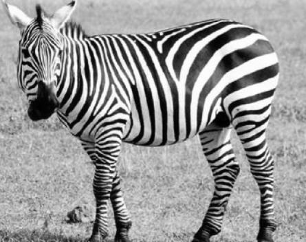
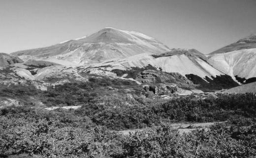
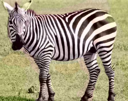
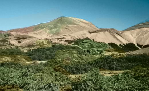
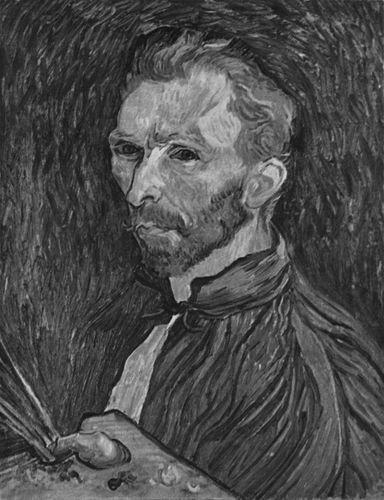
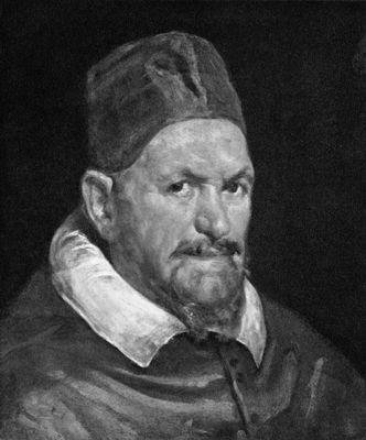
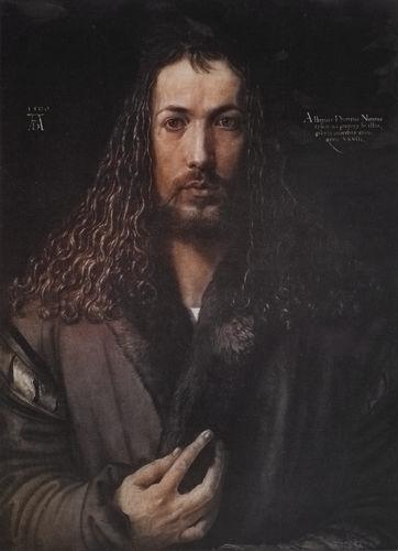
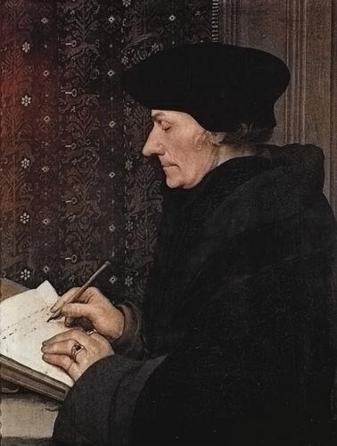
larsson@cs.uchicago.edu, {mmaire,greg}@ttic.edu
Learning Representations for Automatic Colorization
Abstract
We develop a fully automatic image colorization system. Our approach leverages recent advances in deep networks, exploiting both low-level and semantic representations. As many scene elements naturally appear according to multimodal color distributions, we train our model to predict per-pixel color histograms. This intermediate output can be used to automatically generate a color image, or further manipulated prior to image formation. On both fully and partially automatic colorization tasks, we outperform existing methods. We also explore colorization as a vehicle for self-supervised visual representation learning.
1 Introduction
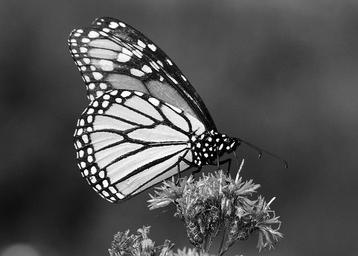
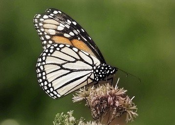
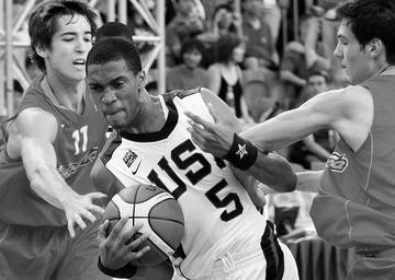
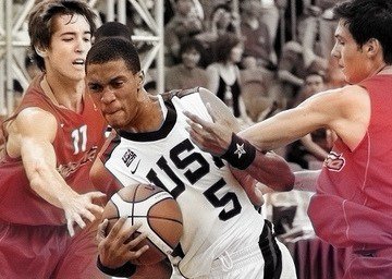
Colorization of grayscale images is a simple task for the human imagination. A human need only recall that sky is blue and grass is green; for many objects, the mind is free to hallucinate several plausible colors. The high-level comprehension required for this process is precisely why the development of fully automatic colorization algorithms remains a challenge. Colorization is thus intriguing beyond its immediate practical utility in graphics applications. Automatic colorization serves as a proxy measure for visual understanding. Our work makes this connection explicit; we unify a colorization pipeline with the type of deep neural architectures driving advances in image classification and object detection.
Both our technical approach and focus on fully automatic results depart from past work. Given colorization’s importance across multiple applications (e.g. historical photographs and videos [41], artist assistance [38, 32]), much research strives to make it cheaper and less time-consuming [42, 22, 20, 3, 27, 6, 14, 7, 5]. However, most methods still require some level of user input [22, 34, 20, 3, 6, 14]. Our work joins the relatively few recent efforts on fully automatic colorization [27, 7, 5]. Some [7, 5] show promising results on typical scenes (e.g. landscapes), but their success is limited on complex images with foreground objects.
[trim=0.1cm 0.1cm 0.1cm 0.1cm]figures/overview
At a technical level, existing automatic colorization methods often employ a strategy of finding suitable reference images and transferring their color onto a target grayscale image [27, 7]. This works well if sufficiently similar reference images can be found, but is difficult for unique grayscale input images. Such a strategy also requires processing a large repository of reference images at test time. In contrast, our approach is free of database search and fast at test time. Section 2 provides a complete view of prior methods, highlighting differences.
Our approach to automatic colorization converts two intuitive observations into design principles. First, semantic information matters. In order to colorize arbitrary images, a system must interpret the semantic composition of the scene (what is in the image: faces, cars, plants, …) as well as localize objects (where things are). Deep convolutional neural networks (CNNs) can serve as tools to incorporate semantic parsing and localization into a colorization system.
Our second observation is that while some scene elements can be assigned a single color with high confidence, others (e.g. clothes or cars) may draw from many suitable colors. Thus, we design our system to predict a color histogram, instead of a single color, at every image location. Figure 2 sketches the CNN architecture we use to connect semantics with color distributions by exploiting features across multiple abstraction levels. Section 3 provides details.
Section 4 experimentally validates our algorithm against competing methods [42, 7] in two settings: fully (grayscale input only) and partially (grayscale input with reference global color histogram) automatic colorization. Across every metric and dataset [43, 31, 33], our method achieves the best performance. Our system’s fully automatic output is superior to that of prior methods relying on additional information such as reference images or ground-truth color histograms. To ease the comparison burden for future research, we propose a new colorization benchmark on ImageNet [33]. We also experiment with colorization itself as an objective for learning visual representations from scratch, thereby replacing use of ImageNet pretraining in a traditional semantic labeling task.
Section 5 summarizes our contributions: (1) a novel technical approach to colorization, bringing semantic knowledge to bear using CNNs, and modeling color distributions; (2) state-of-the-art performance across fully and partially automatic colorization tasks; (3) a new ImageNet colorization benchmark; (4) proof of concept on colorization for self-supervised representation learning.
2 Related work
Previous colorization methods broadly fall into three categories: scribble-based [22, 16, 32, 45, 25], transfer [42, 20, 39, 3, 27, 6, 14], and automatic direct prediction [7, 5].
Scribble-based methods, introduced by Levin et al. [22], require manually specifying desired colors of certain regions. These scribble colors are propagated under the assumption that adjacent pixels with similar luminance should have similar color, with the optimization relying on Normalized Cuts [36]. Users can interactively refine results via additional scribbles. Further advances extend similarity to texture [32, 25], and exploit edges to reduce color bleeding [16].
Transfer-based methods rely on availability of related reference image(s), from which color is transferred to the target grayscale image. Mapping between source and target is established automatically, using correspondences between local descriptors [42, 3, 27], or in combination with manual intervention [20, 6]. Excepting [27], reference image selection is at least partially manual.
In contrast to these method families, our goal is fully automatic colorization. We are aware of two recent efforts in this direction. Deshpande et al. [7] colorize an entire image by solving a linear system. This can be seen as an extension of patch-matching techniques [42], adding interaction terms for spatial consistency. Regression trees address the high-dimensionality of the system. Inference requires an iterative algorithm. Most of the experiments are focused on a dataset (SUN-6) limited to images of a few scene classes, and best results are obtained when the scene class is known at test time. They also examine another partially automatic task, in which a desired global color histogram is provided.
The work of Cheng et al. [5] is perhaps most related to ours. It combines three levels of features with increasing receptive field: the raw image patch, DAISY features [40], and semantic features [24]. These features are concatenated and fed into a three-layer fully connected neural network trained with an loss. Only this last component is optimized; the feature representations are fixed.
Unlike [7, 5], our system does not rely on hand-crafted features, is trained end-to-end, and treats color prediction as a histogram estimation task rather than as regression. Experiments in Section 4 justify these principles by demonstrating performance superior to the best reported by [7, 5] across all regimes.
Two concurrent efforts also present feed-forward networks trained end-to-end for colorization. Iizuka & Simo-Serra et al. [17] propose a network that concatenates two separate paths, specializing in global and local features, respectively. This concatenation can be seen as a two-tiered hypercolumn; in comparison, our 16-layer hypercolumn creates a continuum between low- and high-level features. Their network is trained jointly for classification (cross-entropy) and colorization ( loss in Lab). We initialize, but do not anchor, our system to a classification-based network, allowing for fine-tuning of colorization on unlabeled datasets.
Zhang et al. [46] similarly propose predicting color histograms to handle multi-modality. Some key differences include their usage of up-convolutional layers, deep supervision, and dense training. In comparison, we use a fully convolutional approach, with deep supervision implicit in the hypercolumn design, and, as Section 3 describes, memory-efficient training via spatially sparse samples.
3 Method
We frame the colorization problem as learning a function . Given a grayscale image patch , predicts the color of its center pixel. The patch size is the receptive field of the colorizer. The output space depends on the choice of color parameterization. We implement according to the neural network architecture diagrammed in Figure 2.
Motivating this strategy is the success of similar architectures for semantic segmentation [11, 24, 4, 15, 28] and edge detection [26, 12, 1, 35, 44]. Together with colorization, these tasks can all be viewed as image-to-image prediction problems, in which a value is predicted for each input pixel. Leading methods commonly adapt deep convolutional neural networks pretrained for image classification [33, 37]. Such classification networks can be converted to fully convolutional networks that produce output of the same spatial size as the input, e.g. using the shift-and-stitch method [24] or the more efficient à trous algorithm [4]. Subsequent training with a task-specific loss fine-tunes the converted network.
Skip-layer connections, which directly link low- and mid-level features to prediction layers, are an architectural addition beneficial for many image-to-image problems. Some methods implement skip connections directly through concatenation layers [24, 4], while others equivalently extract per-pixel descriptors by reading localized slices of multiple layers [26, 28, 15]. We use this latter strategy and adopt the recently coined hypercolumn terminology [15] for such slices.
Though we build upon these ideas, our technical approach innovates on two fronts. First, we integrate domain knowledge for colorization, experimenting with output spaces and loss functions. We design the network output to serve as an intermediate representation, appropriate for direct or biased sampling. We introduce an energy minimization procedure for optionally biasing sampling towards a reference image. Second, we develop a novel and efficient computational strategy for network training that is widely applicable to hypercolumn architectures.
3.1 Color spaces
We generate training data by converting color images to grayscale according to . This is only one of many desaturation options and chosen primarily to facilitate comparison with Deshpande et al. [7]. For the representation of color predictions, using RGB is overdetermined, as lightness is already known. We instead consider output color spaces with (or a closely related quantity) conveniently appearing as a separate pass-through channel:
-
•
Hue/chroma. Hue-based spaces, such as HSL, can be thought of as a color cylinder, with angular coordinate (hue), radial distance (saturation), and height (lightness). The values of and are unstable at the bottom (black) and top (white) of the cylinder. HSV describes a similar color cylinder which is only unstable at the bottom. However, is no longer one of the channels. We wish to avoid both instabilities and still retain as a channel. The solution is a color bicone, where chroma () takes the place of saturation. Conversion to HSV is given by .
-
•
Lab and . Lab (or L*a*b) is designed to be perceptually linear. The color vector defines a Euclidean space where the distance to the origin determines chroma. Deshpande et al. [7] use a color space somewhat similar to Lab, denoted “ab”. To differentiate, we call their color space .
3.2 Loss
For any output color representation, we require a loss function for measuring prediction errors. A first consideration, also used in [5], is regression in Lab:
| (1) |
where describes the vector space. However, regression targets do not handle multimodal color distributions well. To address this, we instead predict distributions over a set of color bins, a technique also used in [3]:
| (2) |
where describes a histogram over bins, and is the KL-divergence. The ground-truth histogram is set as the empirical distribution in a rectangular region of size around the center pixel. Somewhat surprisingly, our experiments see no benefit to predicting smoothed histograms, so we simply set . This makes a one-hot vector and Equation (2) the log loss. For histogram predictions, the last layer of neural network is always a softmax.
There are several choices of how to bin color space. We bin the Lab axes by evenly spaced Gaussian quantiles (). They can be encoded separately for and (as marginal distributions), in which case our loss becomes the sum of two separate terms defined by Equation (2). They can also be encoded as a joint distribution over and , in which case we let the quantiles form a 2D grid of bins. In our experiments, we set for marginal distributions and for joint. We determined these numbers, along with , to offer a good compromise of output fidelity and output complexity.
For hue/chroma, we only consider marginal distributions and bin axes uniformly in . Since hue becomes unstable as chroma approaches zero, we add a sample weight to the hue based on the chroma:
| (3) |
where and is the sample pixel’s chroma. We set , roughly the inverse expectation of , thus equally weighting hue and chroma.
3.3 Inference
Given network trained according to a loss function in the previous section, we evaluate it at every pixel in a test image: . For the loss, all that remains is to combine each with the respective lightness and convert to RGB. With histogram predictions, we consider options for inferring a final color:
-
•
Sample Draw a sample from the histogram. If done per pixel, this may create high-frequency color changes in areas of high-entropy histograms.
-
•
Mode Take the as the color. This can create jarring transitions between colors, and is prone to vote splitting for proximal centroids.
-
•
Median Compute cumulative sum of and use linear interpolation to find the value at the middle bin. Undefined for circular histograms, such as hue.
-
•
Expectation Sum over the color bin centroids weighted by the histogram.
For Lab output, we achieve the best qualitative and quantitative results using expectations. For hue/chroma, the best results are achieved by taking the median of the chroma. Many objects can appear both with and without chroma, which means is a particularly common bin. This mode draws the expectation closer to zero, producing less saturated images. As for hue, since it is circular, we first compute the complex expectation:
| (4) |
We then set hue to the argument of remapped to lie in .
In cases where the estimate of the chroma is high and is close to zero, the instability of the hue can create artifacts. A simple, yet effective, fix is chromatic fading: downweight the chroma if the absolute value of is too small. We thus re-define the predicted chroma by multiplying it by a factor of . In our experiments, we set (obtained via cross-validation).
3.4 Histogram transfer from ground-truth
So far, we have only considered the fully automatic color inference task. Deshpande et al. [7], test a separate task where the ground-truth histogram in the two non-lightness color channels of the original color image is made available.111 Note that if the histogram of the channel were available, it would be possible to match lightness to lightness exactly and thus greatly narrow down color placement. In order to compare, we propose two histogram transfer methods. We refer to the predicted image as the source and the ground-truth image as the target.
Lightness-normalized quantile matching. Divide the RGB representation of both source and target by their respective lightness. Compute marginal histograms over the resulting three color channels. Alter each source histogram to fit the corresponding target histogram by quantile matching, and multiply by lightness. Though it does not exploit our richer color distribution predictions, quantile matching beats the cluster correspondence method of [7] (see Table 4).
Energy minimization. We phrase histogram matching as minimizing energy:
| (5) |
where is the number of pixels, are the predicted and posterior distributions, respectively. The target histogram is denoted by . The first term contains unary potentials that anchor the posteriors to the predictions. The second term is a symmetric distance to promote proximity between source and target histograms. Weight defines relative importance of histogram matching. We estimate the source histogram as . We parameterize the posterior for all pixels as: , where the vector can be seen as a global bias for each bin. It is also possible to solve for the posteriors directly; this does not perform better quantitatively and is more prone to introducing artifacts. We solve for using gradient descent on and use the resulting posteriors in place of the predictions. In the case of marginal histograms, the optimization is run twice, once for each color channel.
3.5 Neural network architecture and training
Our base network is a fully convolutional version of VGG-16 [37] with two changes: (1) the classification layer (fc8) is discarded, and (2) the first filter layer (conv1_1) operates on a single intensity channel instead of mean-subtracted RGB. We extract a hypercolumn descriptor for a pixel by concatenating the features at its spatial location in all layers, from data to conv7 (fc7), resulting in a channel descriptor. We feed this hypercolumn into a fully connected layer with channels (h_fc1 in Figure 2), to which we connect output predictors.
Processing each pixel separately in such manner is quite costly. We instead run an entire image through a single forward pass of VGG-16 and approximate hypercolumns using bilinear interpolation. Even with such sharing, densely extracting hypercolumns requires significant memory ( GB for input).
Input

Our Method
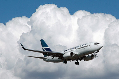
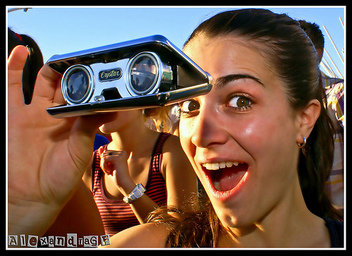
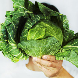
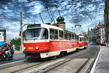
Ground-truth
Input
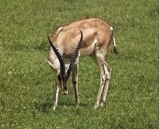


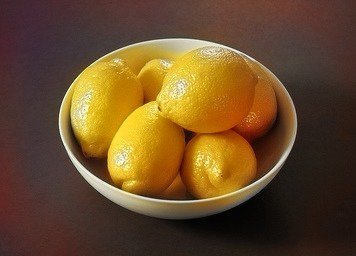
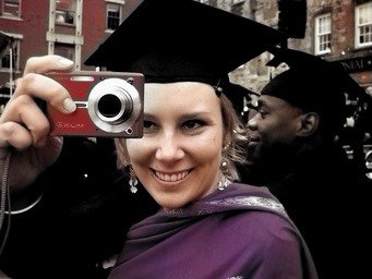
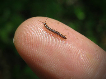
Our Method
Ground-truth
To fit image batches in memory during training, we instead extract hypercolumns at only a sparse set of locations, implementing a custom Caffe [21] layer to directly compute them.222 https://github.com/gustavla/autocolorize Extracting batches of only hypercolumn descriptors per input image, sampled at random locations, provides sufficient training signal. In the backward pass of stochastic gradient descent, an interpolated hypercolumn propagates its gradients to the four closest spatial cells in each layer. Locks ensure atomicity of gradient updates, without incurring any performance penalty. This drops training memory for hypercolumns to only MB per image.
We initialize with a version of VGG-16 pretrained on ImageNet, adapting it to grayscale by averaging over color channels in the first layer and rescaling appropriately. Prior to training for colorization, we further fine-tune the network for one epoch on the ImageNet classification task with grayscale input. As the original VGG-16 was trained without batch normalization [18], scale of responses in internal layers can vary dramatically, presenting a problem for learning atop their hypercolumn concatenation. Liu et al. [23] compensate for such variability by applying layer-wise normalization. We use the alternative of balancing hypercolumns so that each layer has roughly unit second moment (); Appendix (Section 0.A.1) provides additional details.








Grayscale only
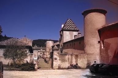

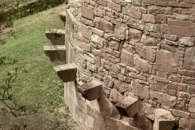
GT Histogram
Our Method
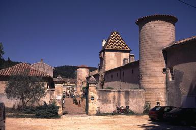

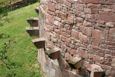
Ground-truth
4 Experiments
Starting from pretrained VGG-16-Gray, described in the previous section, we attach h_fc1 and output prediction layers with Xavier initialization [13], and fine-tune the entire system for colorization. We consider multiple prediction layer variants: Lab output with loss, and both Lab and hue/chroma marginal or joint histogram output with losses according to Equations (2) and (3). We train each system variant end-to-end for one epoch on the million images of the ImageNet training set, each resized to at most pixels in smaller dimension. A single epoch takes approximately 17 hours on a GTX Titan X GPU. At test time, colorizing a single pixel image takes seconds.
| ModelMetric | RMSE | PSNR |
|---|---|---|
| No colorization | 0.343 | 22.98 |
| Lab, | 0.318 | 24.25 |
| Lab, | 0.321 | 24.33 |
| Lab, | 0.328 | 24.30 |
| Hue/chroma, | 0.342 | 23.77 |
| + chromatic fading | 0.299 | 24.45 |
| ModelMetric | RMSE | PSNR |
|---|---|---|
| data..fc7 | 0.299 | 24.45 |
| data..conv5_3 | 0.306 | 24.13 |
| conv4_1..fc7 | 0.302 | 24.45 |
| conv5_1..fc7 | 0.307 | 24.38 |
| fc6..fc7 | 0.323 | 24.22 |
| fc7 | 0.324 | 24.19 |
We setup two disjoint subsets of the ImageNet validation data for our own use: validation images (cval1k) and test images (ctest10k). Each set has a balanced representation for ImageNet categories, and excludes any images encoded as grayscale, but may include images that are naturally grayscale (e.g. closeup of nuts and bolts), where an algorithm should know not to add color. Category labels are discarded; only images are available at test time. We propose ctest10k as a standard benchmark with the following metrics:
-
•
RMSE: root mean square error in averaged over all pixels [7].
- •
By virtue of comparing to ground-truth color images, quantitative colorization metrics can penalize reasonable, but incorrect, color guesses for many objects (e.g. red car instead of blue car) more than jarring artifacts. This makes qualitative results for colorization as important as quantitative; we report both.
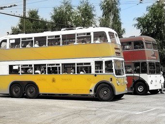
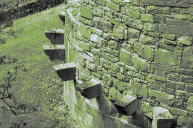
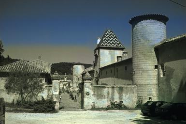
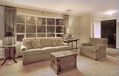
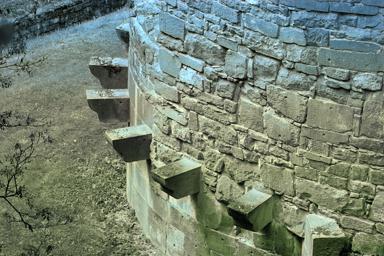
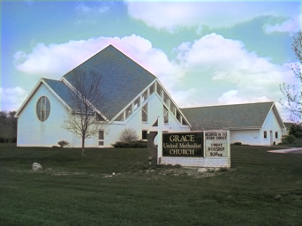
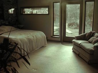
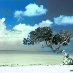
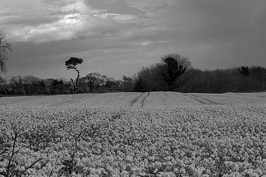
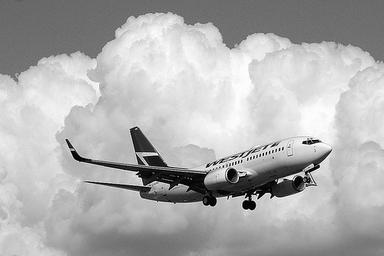
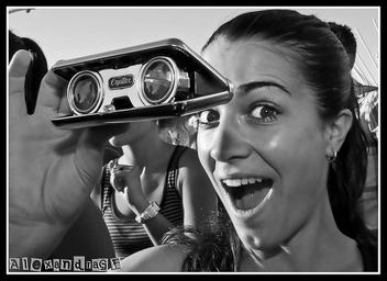
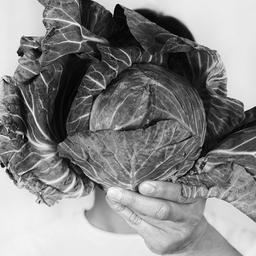
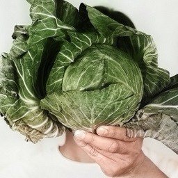
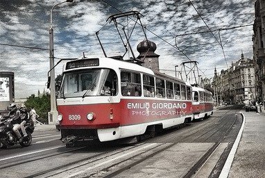
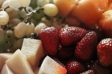
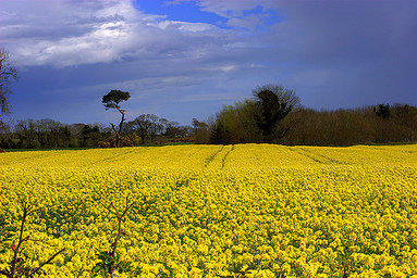
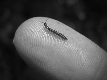
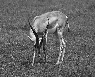
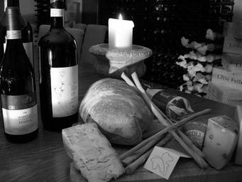
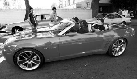
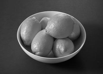
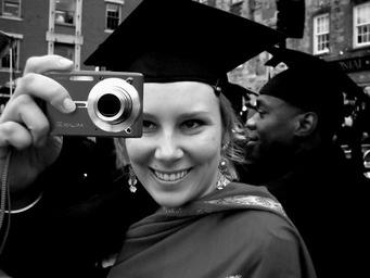
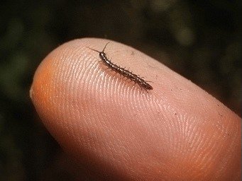
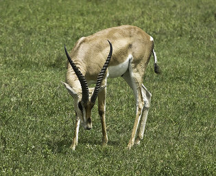
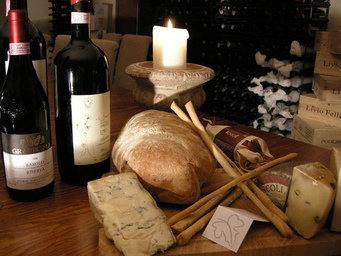
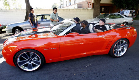
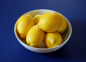
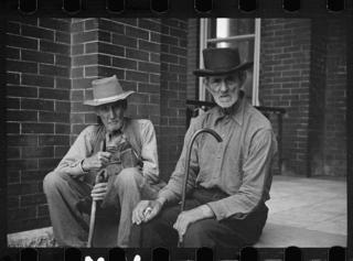
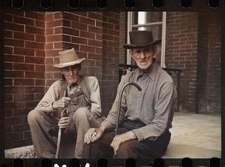
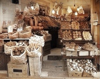
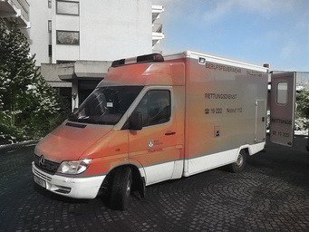
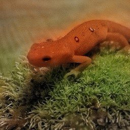
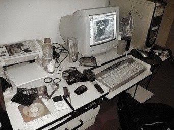
Figures Learning Representations for Automatic Colorization, 3, and 4 show example test results of our best system variant, selected according to performance on the validation set and trained for a total of epochs. This variant predicts hue and chroma and uses chromatic fading during image generation. Table 2 provides validation benchmarks for all system variants, including the trivial baseline of no colorization. On ImageNet test (ctest10k), our selected model obtains (RMSE, , avg/px) and dB (PSNR, RGB, avg/im), compared to and dB for the baseline.
Table 2 examines the importance of different neural network layers to colorization; it reports validation performance of ablated systems that include only the specified subsets of layers in the hypercolumn used to predict hue and chroma. Some lower layers may be discarded without much performance loss, yet higher layers alone (fc6..fc7) are insufficient for good colorization.
Our ImageNet colorization benchmark is new to a field lacking an established evaluation protocol. We therefore focus on comparisons with two recent papers [7, 5], using their self-defined evaluation criteria. To do so, we run our ImageNet-trained hue and chroma model on two additional datasets:
-
•
SUN-A [31] is a subset of the SUN dataset [43] containing object categories. Cheng et al. [5] train a colorization system on images and report results on test images. We were unable to obtain the list of test images, and therefore report results averaged over five random subsets of SUN-A images. We do not use any SUN-A images for training.
-
•
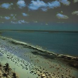
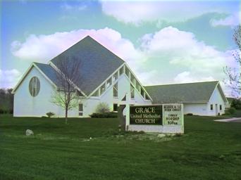
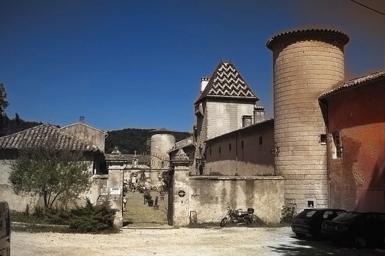
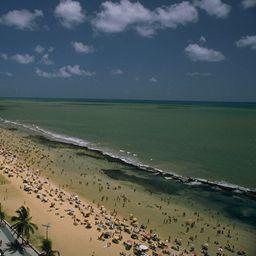
SUN-6, another SUN subset, used by Deshpande et al. [7], includes images from scene categories (beach, castle, outdoor, kitchen, living room, bedroom). We compare our results on test images to those reported in [7] for their method as well as for Welsh et al. [42] with automatically matched reference images as in [27]. Following [7], we consider another evaluation regime in which ground-truth target color histograms are available.
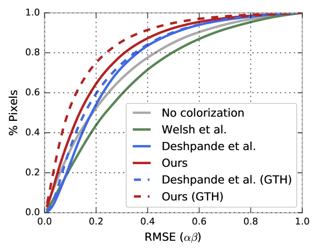
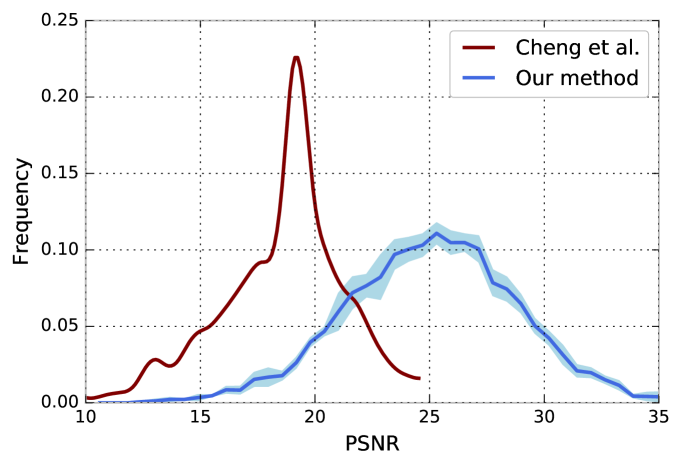
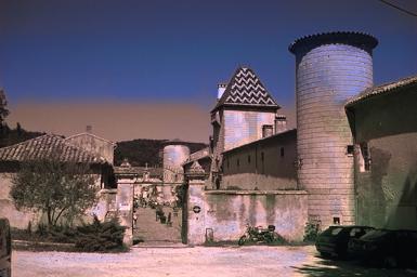
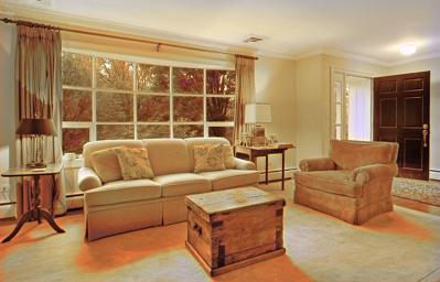
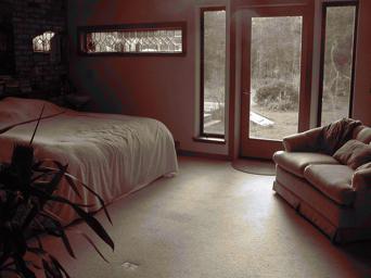
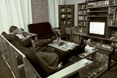
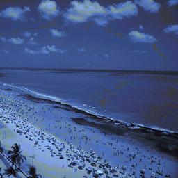
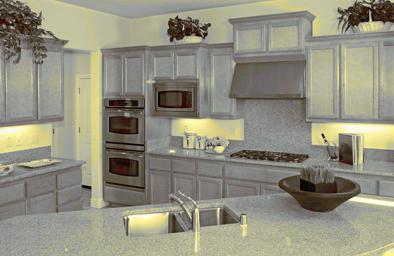
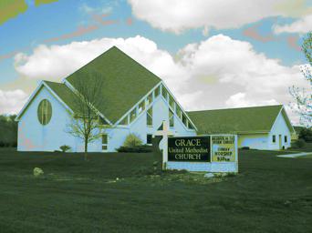
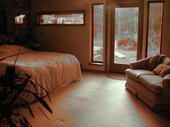
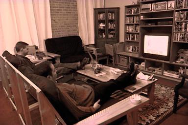
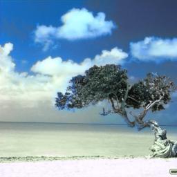
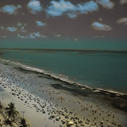
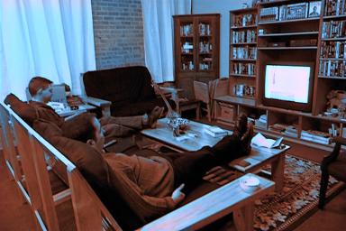
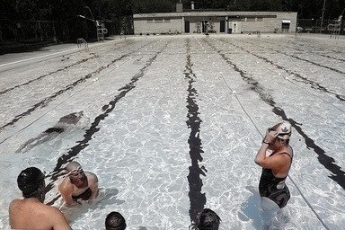
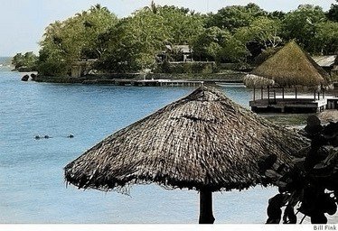
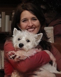
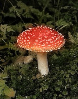
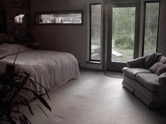
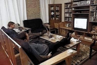
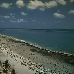
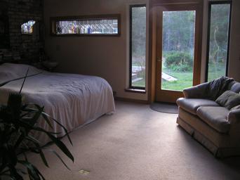
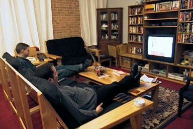
Figure 5 shows a comparison of results on SUN-6. Forgoing usage of ground-truth global histograms, our fully automatic system produces output qualitatively superior to methods relying on such side information. Tables 4 and 4 report quantitative performance corroborating this view. The partially automatic systems in Table 4 adapt output to fit global histograms using either: (C) cluster correspondences [7], (Q) quantile matching, or (E) our energy minimization described in Section 3.4. Our quantile matching results are superior to those of [7] and our new energy minimization procedure offers further improvement.
Figures 7 and 7 compare error distributions on SUN-6 and SUN-A. As in Table 4, our fully automatic method dominates all competing approaches, even those which use auxiliary information. It is only outperformed by the version of itself augmented with ground-truth global histograms. On SUN-A, Figure 7 shows clear separation between our method and [5] on per-image PSNR.
The Appendix (Figures 14 and 15) provides anecdotal comparisons to one additional method, that of Charpiat et al. [2], which can be considered an automatic system if reference images are available. Unfortunately, source code of [2] is not available and reported time cost is prohibitive for large-scale evaluation ( minutes per image). We were thus unable to benchmark [2] on large datasets.
With regard to concurrent work, Zhang et al. [46] include a comparison of our results to their own. The two systems are competitive in terms of quantitative measures of colorization accuracy. Their system, set to produce more vibrant colors, has an advantage in terms of human-measured preferences. In contrast, an off-the-shelf VGG-16 network for image classification, consuming our system’s color output, more often produces correct labels, suggesting a realism advantage. We refer interested readers to [46] for the full details of this comparison.
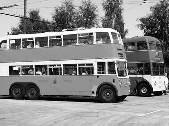
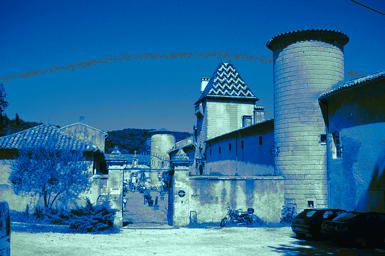
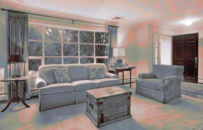
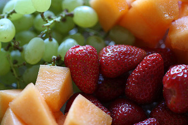
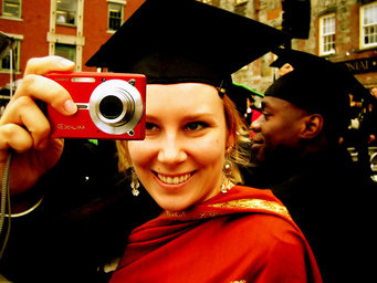
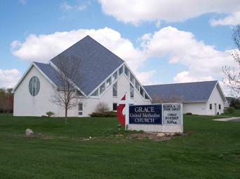
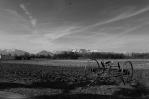
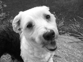
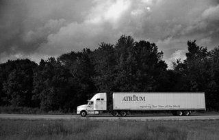
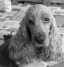
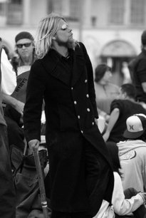
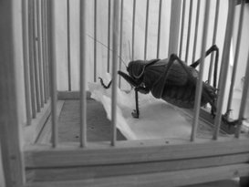
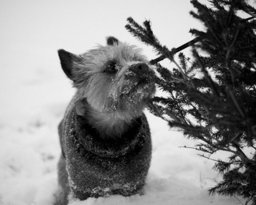
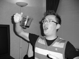
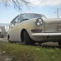
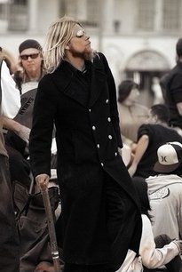
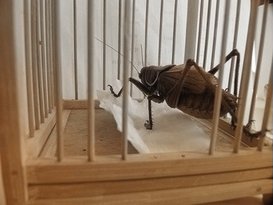
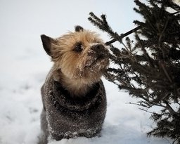
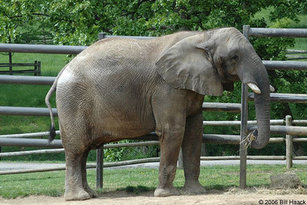
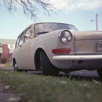
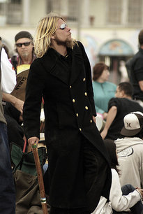
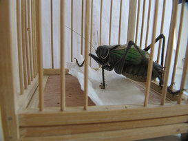
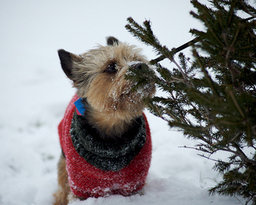
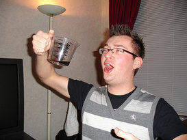
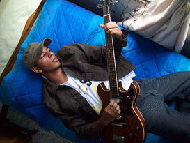
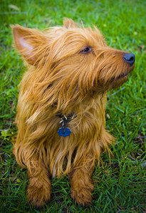
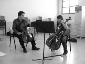
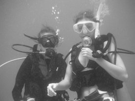
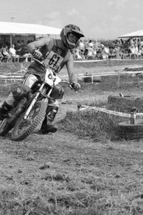
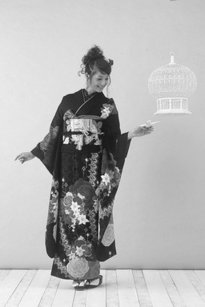
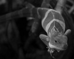
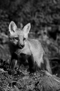
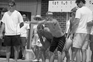
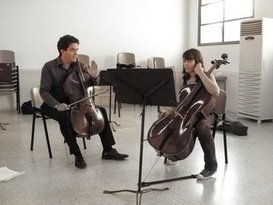
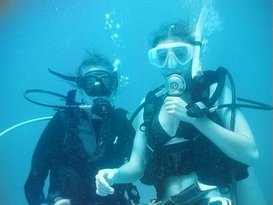
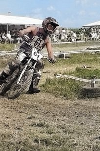
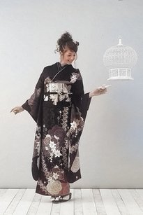
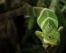
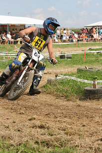
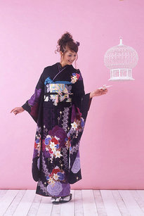
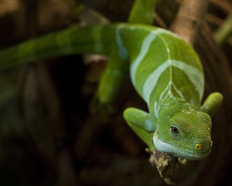
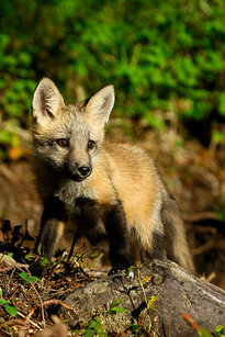
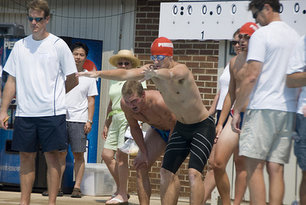
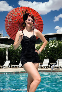
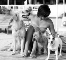
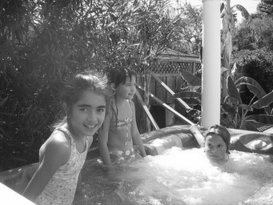
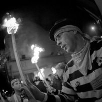
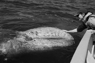
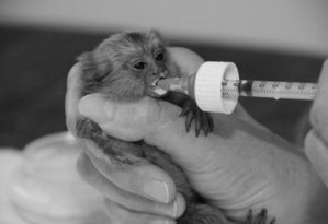
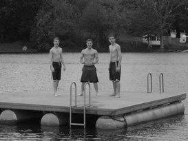
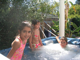
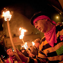
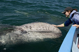
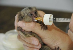
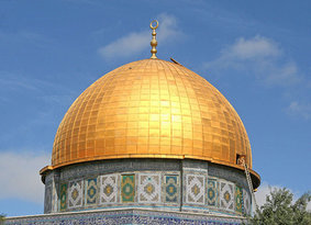
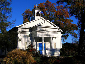
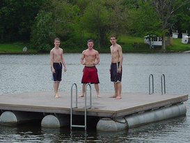
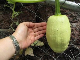
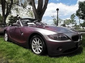
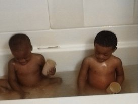
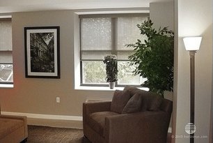
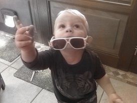
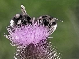
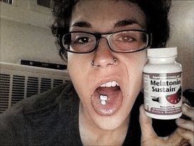
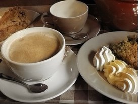
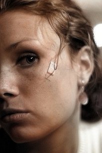
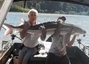
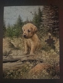
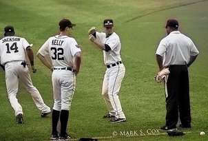
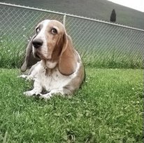
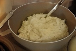
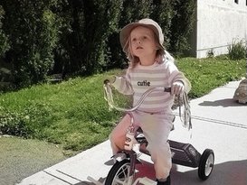
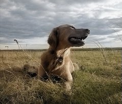
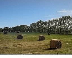
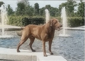
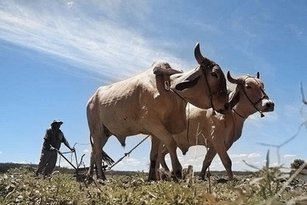
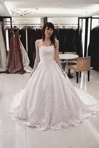
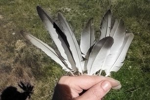
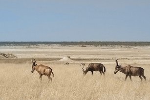
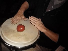
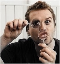
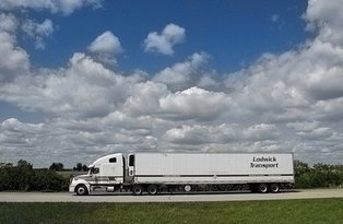
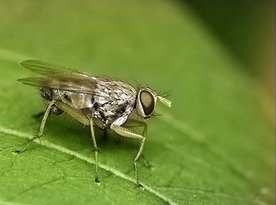
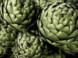
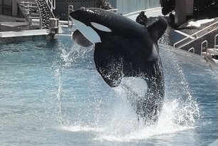
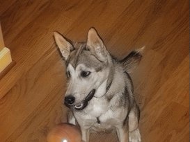
Though we achieve significant improvements over prior state-of-the-art, our results are not perfect. Figure 8 shows examples of significant failures. Minor imperfections are also present in some of the results in Figures 3 and 4. We believe a common failure mode correlates with gaps in semantic interpretation: incorrectly identified or unfamiliar objects and incorrect segmentation. In addition, there are “mistakes” due to natural uncertainty of color – e.g. the graduation robe at the bottom right of Figure 3 is red, but could as well be purple.
Since our method produces histograms, we can provide interactive means of biasing colorizations according to user preferences. Rather than output a single color per pixel, we can sample color for image regions and evaluate color uncertainty. Specifically, solving our energy minimization formulation (Equation (5)) with global biases that are not optimized based on a reference image, but simply “rotated” through color space, induces changed color preferences throughout the image. The uncertainty in the predicted histogram modulates this effect.
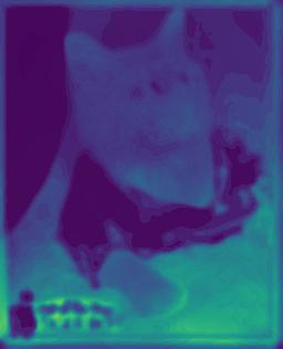
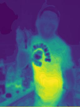
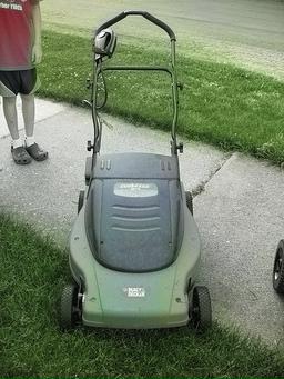
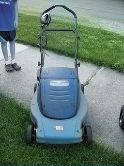
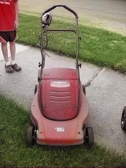
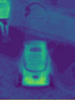
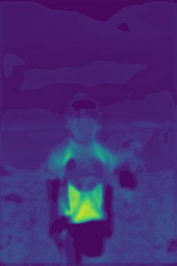
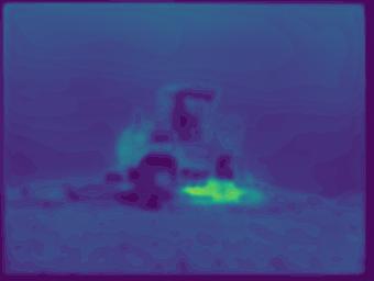
Figure 9 shows multiple sampled colorizations, together with a visualization of uncertainty. Here, uncertainty is the entropy of the predicted hue multiplied by the chroma. Our distributional output and energy minimization framework open the path for future investigation of human-in-the-loop colorization tools.
4.1 Representation learning
 |
 |
 |
 |
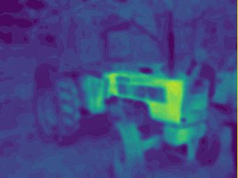 |
High-level visual understanding is essential for the colorization of grayscale images, motivating our use of an ImageNet pretrained network as a starting point. But with enough training data, perhaps we can turn this around and use colorization as means of learning networks for capturing high-level visual representations. Table 6 shows that a colorization network, trained from scratch using only unlabeled color images, is surprisingly competitive. It converges slower, but requires not more than twice the number of epochs.
Our preliminary work shows that the networks learned via training colorization from scratch generalize well to other visual tasks. This is significant because such training requires no human annotation effort. It follows a recent trend of learning representations through self-supervision (e.g. context prediction [8], solving jigsaw puzzles [29], inpainting [30], adversarial feature learning [9, 10]).
We examine self-supervised colorization as a replacement for supervised ImageNet pretraining on the Pascal VOC 2012 semantic segmentation task, with results on grayscale validation set images. We train colorization from scratch on ImageNet (Table 6) and fine-tune for Pascal semantic segmentation. We make the one adjustment of employing cross-validated early stopping to avoid overfitting. Table 6 shows this strategy to be promising as a drop-in replacement for supervised ImageNet pretraining. Self-supervised colorization more than halfway bridges the gap between random initialization and supervised pretraining.
As VGG-16 is a more performant architecture, comparison with prior work is not straightforward. Yet, Table 6 still indicates that colorization is a front-runner among the self-supervision methods, leading to an 18-point improvement in mIU over the baseline. To our knowledge, 50.2% is the highest reported result that does not supplement training with additional annotated data [19].
| Initialization | RMSE | PSNR |
|---|---|---|
| Classifier | 0.299 | 24.45 |
| Random | 0.311 | 24.25 |
| Initialization | Architecture | mIU (%) | |||
| Classifier | VGG-16 | ✓ | ✓ | 64.0 | |
| Colorizer | VGG-16 | ✓ | 50.2 | ||
| Random | VGG-16 | 32.5 | |||
| Classifier [9, 30] | AlexNet | ✓ | ✓ | ✓ | 48.0 |
| BiGAN [9] | AlexNet | ✓ | ✓ | 34.9 | |
| Inpainter [30] | AlexNet | ✓ | ✓ | 29.7 | |
| Random [30] | AlexNet | ✓ | 19.8 |
5 Conclusion
We present a system that demonstrates state-of-the-art ability to automatically colorize grayscale images. Two novel contributions enable this progress: a deep neural architecture that is trained end-to-end to incorporate semantically meaningful features of varying complexity into colorization, and a color histogram prediction framework that handles uncertainty and ambiguities inherent in colorization while preventing jarring artifacts. Our fully automatic colorizer produces strong results, improving upon previously leading methods by large margins on all datasets tested; we also propose a new large-scale benchmark for automatic image colorization, and establish a strong baseline with our method to facilitate future comparisons. Our colorization results are visually appealing even on complex scenes, and allow for effective post-processing with creative control via color histogram transfer and intelligent, uncertainty-driven color sampling. We further reveal colorization as a promising avenue for self-supervised visual learning.
Acknowledgements. We thank Ayan Chakrabarti for suggesting lightness-normalized quantile matching and for useful discussions, and Aditya Deshpande and Jason Rock for discussions on their work. We gratefully acknowledge the support of NVIDIA Corporation with the donation of GPUs for this research.
References
- [1] Bertasius, G., Shi, J., Torresani, L.: Deepedge: A multi-scale bifurcated deep network for top-down contour detection. In: CVPR (2015)
- [2] Charpiat, G., Bezrukov, I., Altun, Y., Hofmann, M., Schölkopf, B.: Machine learning methods for automatic image colorization. In: Computational Photography: Methods and Applications. CRC Press (2010)
- [3] Charpiat, G., Hofmann, M., Schölkopf, B.: Automatic image colorization via multimodal predictions. In: ECCV (2008)
- [4] Chen, L.C., Papandreou, G., Kokkinos, I., Murphy, K., Yuille, A.L.: Semantic image segmentation with deep convolutional nets and fully connected crfs. In: ICLR (2015)
- [5] Cheng, Z., Yang, Q., Sheng, B.: Deep colorization. In: ICCV (2015)
- [6] Chia, A.Y.S., Zhuo, S., Gupta, R.K., Tai, Y.W., Cho, S.Y., Tan, P., Lin, S.: Semantic colorization with internet images. ACM Transactions on Graphics (TOG) 30(6) (2011)
- [7] Deshpande, A., Rock, J., Forsyth, D.: Learning large-scale automatic image colorization. In: ICCV (2015)
- [8] Doersch, C., Gupta, A., Efros, A.A.: Unsupervised visual representation learning by context prediction. In: Proceedings of the IEEE International Conference on Computer Vision. pp. 1422–1430 (2015)
- [9] Donahue, J., Krähenbühl, P., Darrell, T.: Adversarial feature learning. In: ICLR (2017)
- [10] Dumoulin, V., Belghazi, I., Poole, B., Lamb, A., Arjovsky, M., Mastropietro, O., Courville, A.: Adversarially learned inference. arXiv preprint arXiv:1606.00704 (2016)
- [11] Farabet, C., Couprie, C., Najman, L., LeCun, Y.: Learning hierarchical features for scene labeling. Pattern Analysis and Machine Intelligence, IEEE Transactions on 35(8) (2013)
- [12] Ganin, Y., Lempitsky, V.S.: N-fields: Neural network nearest neighbor fields for image transforms. In: ACCV (2014)
- [13] Glorot, X., Bengio, Y.: Understanding the difficulty of training deep feedforward neural networks. In: AISTATS (2010)
- [14] Gupta, R.K., Chia, A.Y.S., Rajan, D., Ng, E.S., Zhiyong, H.: Image colorization using similar images. In: ACM international conference on Multimedia (2012)
- [15] Hariharan, B., an R. Girshick, P.A., Malik, J.: Hypercolumns for object segmentation and fine-grained localization. CVPR (2015)
- [16] Huang, Y.C., Tung, Y.S., Chen, J.C., Wang, S.W., Wu, J.L.: An adaptive edge detection based colorization algorithm and its applications. In: ACM international conference on Multimedia (2005)
- [17] Iizuka, S., Simo-Serra, E., Ishikawa, H.: Let there be Color!: Joint End-to-end Learning of Global and Local Image Priors for Automatic Image Colorization with Simultaneous Classification. ACM Transactions on Graphics (Proc. of SIGGRAPH 2016) 35(4) (2016)
- [18] Ioffe, S., Szegedy, C.: Batch normalization: Accelerating deep network training by reducing internal covariate shift. In: ICML (2015)
- [19] Ion, A., Carreira, J., Sminchisescu, C.: Probabilistic joint image segmentation and labeling by figure-ground composition. International journal of computer vision 107(1), 40–57 (2014)
- [20] Irony, R., Cohen-Or, D., Lischinski, D.: Colorization by example. In: Eurographics Symp. on Rendering (2005)
- [21] Jia, Y., Shelhamer, E., Donahue, J., Karayev, S., Long, J., Girshick, R., Guadarrama, S., Darrell, T.: Caffe: Convolutional architecture for fast feature embedding. arXiv preprint arXiv:1408.5093 (2014)
- [22] Levin, A., Lischinski, D., Weiss, Y.: Colorization using optimization. ACM Transactions on Graphics (TOG) 23(3) (2004)
- [23] Liu, W., Rabinovich, A., Berg, A.C.: Parsenet: Looking wider to see better. arXiv preprint arXiv:1506.04579 (2015)
- [24] Long, J., Shelhamer, E., Darrell, T.: Fully convolutional networks for semantic segmentation. In: CVPR (2015)
- [25] Luan, Q., Wen, F., Cohen-Or, D., Liang, L., Xu, Y.Q., Shum, H.Y.: Natural image colorization. In: Eurographics conference on Rendering Techniques (2007)
- [26] Maire, M., Yu, S.X., Perona, P.: Reconstructive sparse code transfer for contour detection and semantic labeling. In: ACCV (2014)
- [27] Morimoto, Y., Taguchi, Y., Naemura, T.: Automatic colorization of grayscale images using multiple images on the web. In: SIGGRAPH: Posters (2009)
- [28] Mostajabi, M., Yadollahpour, P., Shakhnarovich, G.: Feedforward semantic segmentation with zoom-out features. In: CVPR (2015)
- [29] Noroozi, M., Favaro, P.: Unsupervised learning of visual representations by solving jigsaw puzzles. In: ECCV (2016)
- [30] Pathak, D., Krahenbuhl, P., Donahue, J., Darrell, T., Efros, A.A.: Context encoders: Feature learning by inpainting. In: CVPR (2016)
- [31] Patterson, G., Xu, C., Su, H., Hays, J.: The sun attribute database: Beyond categories for deeper scene understanding. International Journal of Computer Vision 108(1-2) (2014)
- [32] Qu, Y., Wong, T.T., Heng, P.A.: Manga colorization. ACM Transactions on Graphics (TOG) 25(3) (2006)
- [33] Russakovsky, O., Deng, J., Su, H., Krause, J., Satheesh, S., Ma, S., Huang, Z., Karpathy, A., Khosla, A., Bernstein, M., Berg, A.C., Fei-Fei, L.: ImageNet Large Scale Visual Recognition Challenge. International Journal of Computer Vision (IJCV) 115(3) (2015)
- [34] Sapiro, G.: Inpainting the colors. In: ICIP (2005)
- [35] Shen, W., Wang, X., Wang, Y., Bai, X., Zhang, Z.: Deepcontour: A deep convolutional feature learned by positive-sharing loss for contour detection. In: CVPR (2015)
- [36] Shi, J., Malik, J.: Normalized cuts and image segmentation. Pattern Analysis and Machine Intelligence, IEEE Transactions on 22(8) (2000)
- [37] Simonyan, K., Zisserman, A.: Very deep convolutional networks for large-scale image recognition. In: ICLR (2015)
- [38] Sỳkora, D., Buriánek, J., Žára, J.: Unsupervised colorization of black-and-white cartoons. In: International symposium on Non-photorealistic animation and rendering (2004)
- [39] Tai, Y.W., Jia, J., Tang, C.K.: Local color transfer via probabilistic segmentation by expectation-maximization. In: CVPR (2005)
- [40] Tola, E., Lepetit, V., Fua, P.: A fast local descriptor for dense matching. In: CVPR (2008)
- [41] Tsaftaris, S.A., Casadio, F., Andral, J.L., Katsaggelos, A.K.: A novel visualization tool for art history and conservation: Automated colorization of black and white archival photographs of works of art. Studies in Conservation 59(3) (2014)
- [42] Welsh, T., Ashikhmin, M., Mueller, K.: Transferring color to greyscale images. ACM Transactions on Graphics (TOG) 21(3) (2002)
- [43] Xiao, J., Hays, J., Ehinger, K.A., Oliva, A., Torralba, A.: Sun database: Large-scale scene recognition from abbey to zoo. In: CVPR (2010)
- [44] Xie, S., Tu, Z.: Holistically-nested edge detection. In: ICCV (2015)
- [45] Yatziv, L., Sapiro, G.: Fast image and video colorization using chrominance blending. Image Processing, IEEE Transactions on 15(5) (2006)
- [46] Zhang, R., Isola, P., Efros, A.A.: Colorful image colorization. In: ECCV (2016)
figures/field
Appendix 0.A provides additional training and evaluation details. This is followed by more results and examples in Appendix 0.B.
Appendix 0.A Supplementary details
0.A.1 Re-balancing
To adjust the scale of the activations of layer by factor , without changing any other layer’s activation, the weights and the bias are updated according to:
| (6) |
The activation of becomes:
| (7) |
The inside the ReLU will not affect whether or not a value is rectified, so the two cases remain the same: (1) negative: the activation will be the corresponding feature in regardless of , and (2) positive: the ReLU becomes the identity function and and cancel to get back the original activation.
We set , estimated for each layer separately.
0.A.2 Color space
0.A.3 Error metrics
For images, each image with pixels, we calculate the error metrics as:
| (9) | ||||
| (10) |
Where and for all .
figures/parrot
0.A.4 Lightness correction
Ideally the lightness is an unaltered pass-through channel. However, due to subtle differences in how is defined, it is possible that the lightness of the predicted image, , does not agree with the input, . To compensate for this, we add to all color channels in the predicted RGB image as a final corrective step.
Appendix 0.B Supplementary results
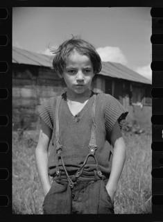
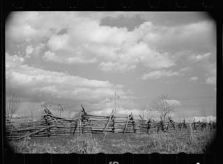
0.B.1 Validation
A more detailed list of validation results for hue/chroma inference methods is seen in Table 7.
[\capbeside\thisfloatsetup capbesideposition=right,top,capbesidewidth=5cm]figure[\FBwidth] Hue Chroma CF RMSE PSNR Sample Sample 0.426 21.41 Mode Mode 0.304 23.90 Expectation Expectation 0.374 23.13 Expectation Expectation ✓ 0.307 24.35 Expectation Median 0.342 23.77 Expectation Median ✓ 0.299 24.45
0.B.2 Examples
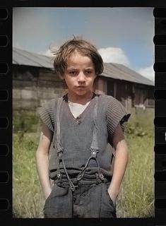
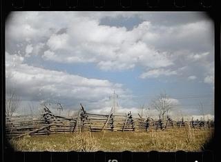
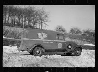
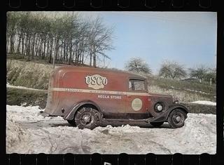
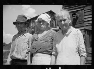
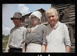
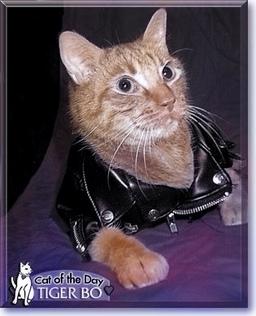
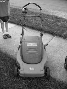
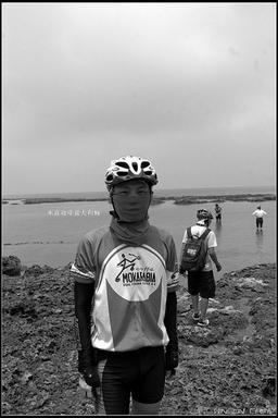
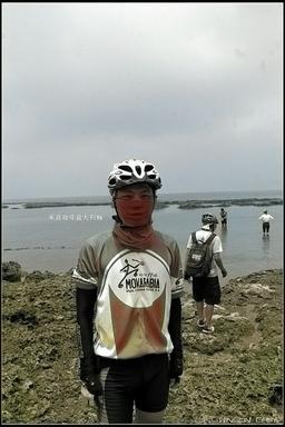
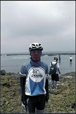
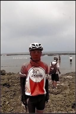
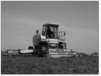
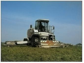
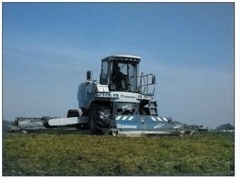
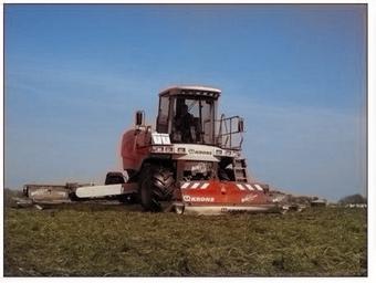
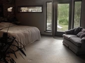
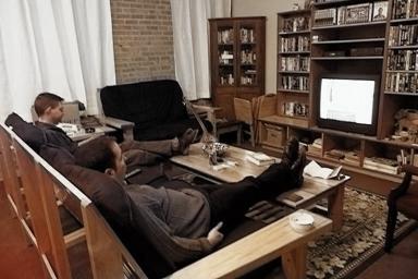
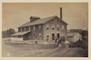
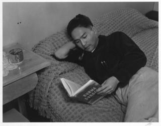
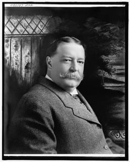
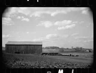
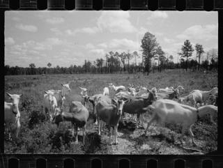
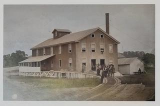
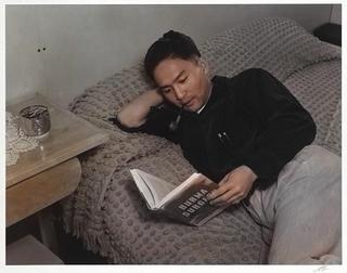
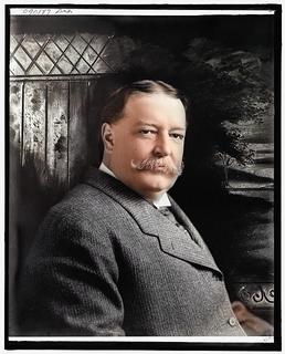
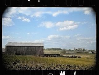
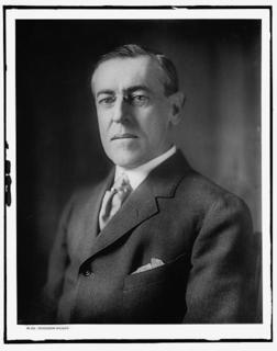
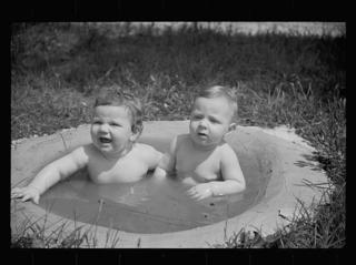
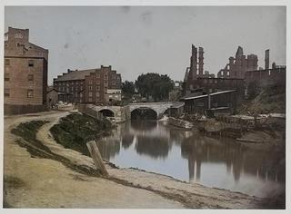
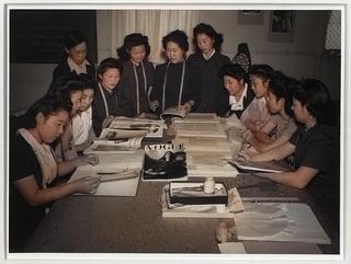
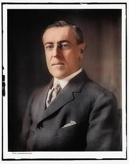
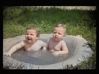
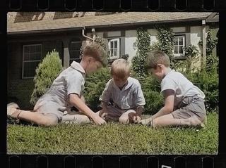
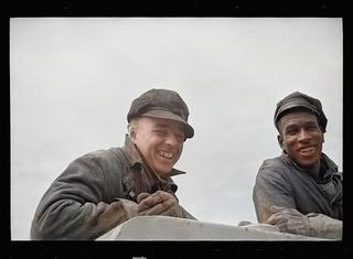
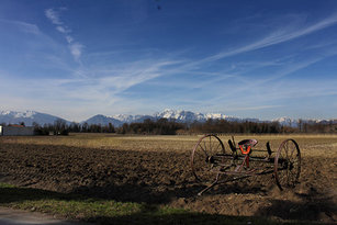
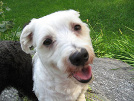
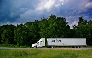
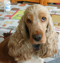
We provide additional samples for global biasing (Figure 12) and SUN-6 (Figure 13). Comparisons with Charpiat et al. [2] appear in Figures 14 and 15. Examples of how our algorithm can bring old photographs to life in Figure 16. More examples on ImageNet (ctest10k) in Figures 17 to 20 and Figure 21 (failure cases). Examples of histogram predictions in Figures 10 and 11.
 |
 |
 |
 |
 |
 |
 |
 |
 |
 |
 |
 |
 |
 |
 |
 |
 |
 |
 |
 |
 |
 |
 |
 |
 |


Grayscale only



GT Histogram
Our Method


Ground-truth

Input
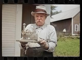
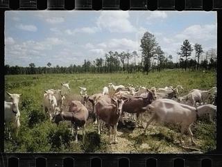
Our Method
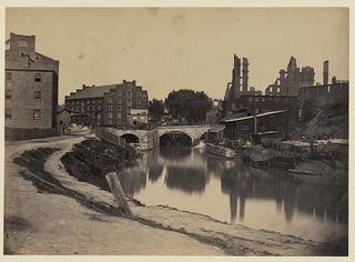
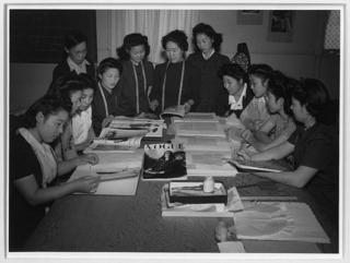


Input
Our Method


Input
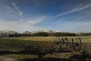
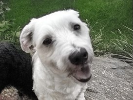
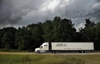
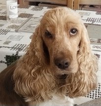


Our Method
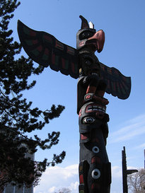
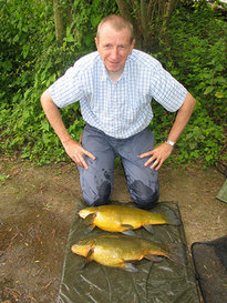
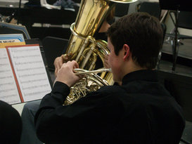
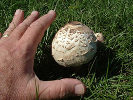
Ground-truth

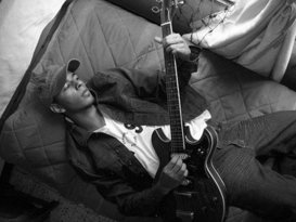
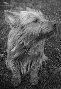
Input
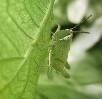
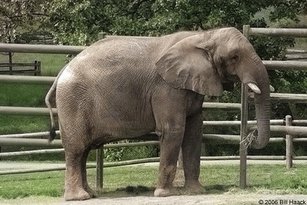
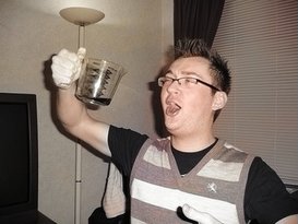
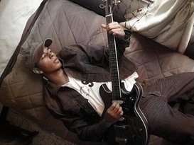
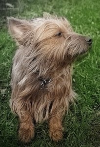
Our Method
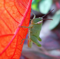
Ground-truth

Input

Our Method
Ground-truth



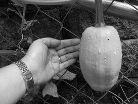

Input
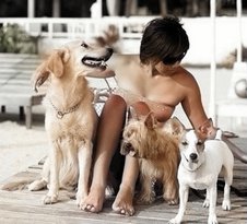


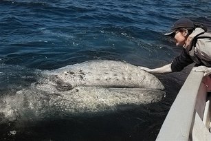
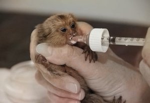



Our Method


Ground-truth
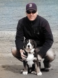
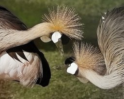
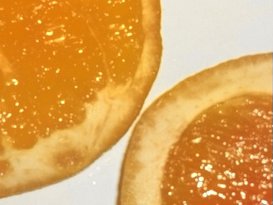

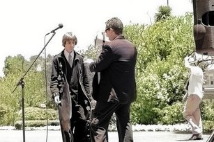
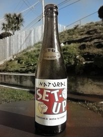
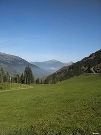
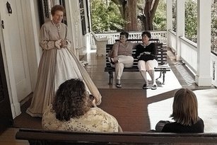
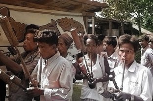
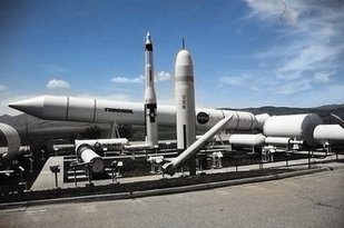


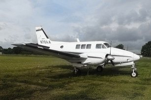
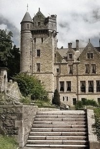
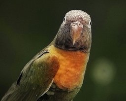
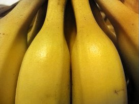
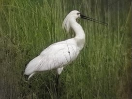
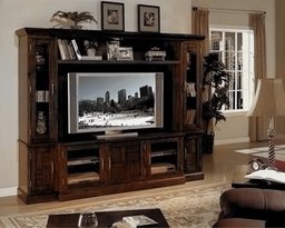
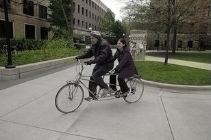
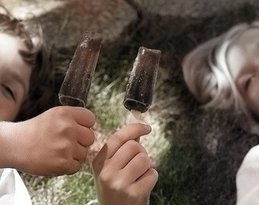
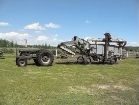
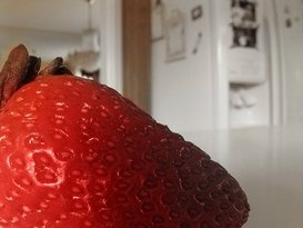
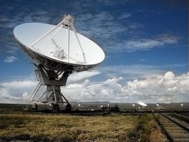
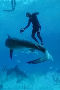


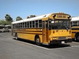
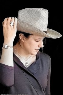
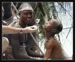
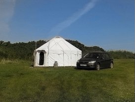
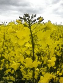
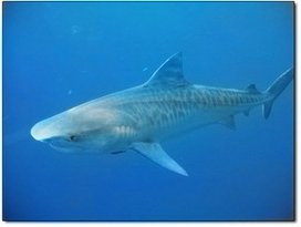
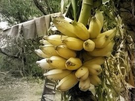
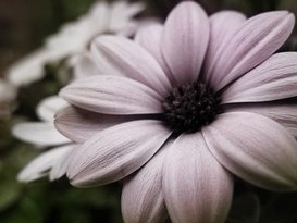
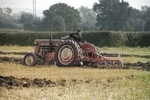
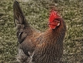
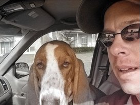

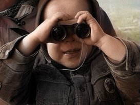
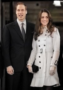
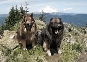
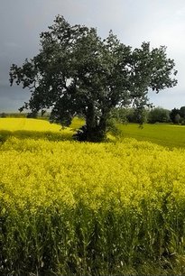
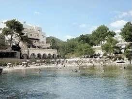
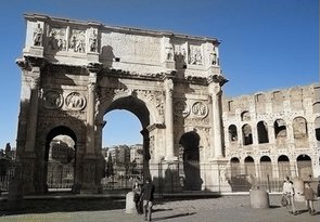

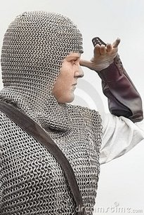
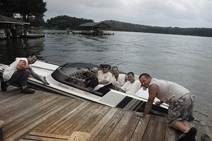


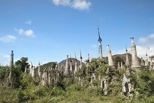
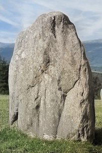

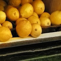


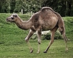
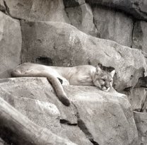
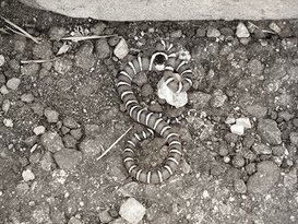
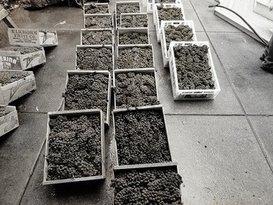
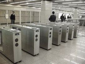
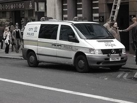
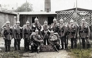

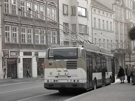
Too Desaturated
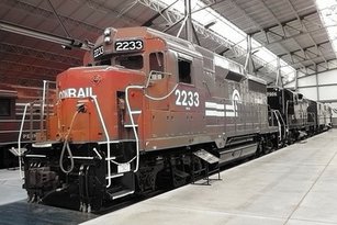
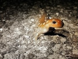
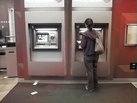
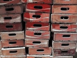
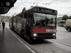

Inconsistent Chroma
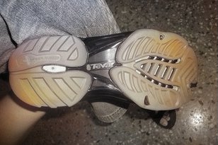
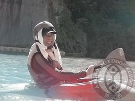

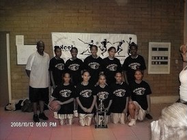
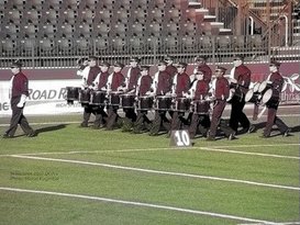
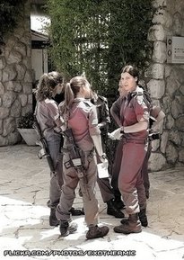
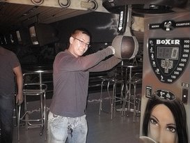
Inconsistent Hue
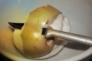

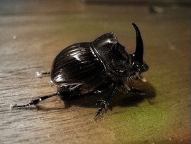
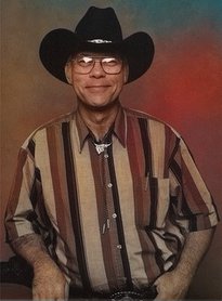
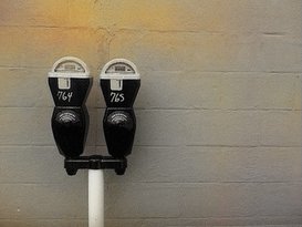

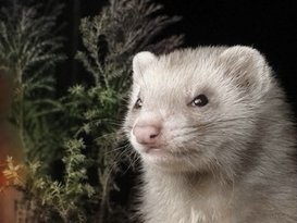
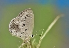
Edge Pollution



Color Bleeding
Appendix 0.C Document changelog
Overview of document revisions:
-
v1
Initial release.
-
v2
ECCV 2016 camera-ready version. Includes discussion about concurrent work and new experiments using colorization to learn visual representations (Section 4.1).
-
v3
Added overlooked reference.
