Properties of Carbon-Oxygen White Dwarfs From Monte Carlo Stellar Models

Abstract

We investigate properties of carbon-oxygen white dwarfs with respect to the composite uncertainties in the reaction rates using the stellar evolution toolkit, Modules for Experiments in Stellar Astrophysics (MESA) and the probability density functions in the reaction rate library STARLIB. These are the first Monte Carlo stellar evolution studies that use complete stellar models. Focusing on 3 M_⊙ models evolved from the pre main-sequence to the first thermal pulse, we survey the remnant core mass, composition, and structure properties as a function of 26 STARLIB reaction rates covering hydrogen and helium burning using a Principal Component Analysis and Spearman Rank-Order Correlation. Relative to the arithmetic mean value, we find the width of the 95% confidence interval to be $\Delta M_{{\rm 1TP}}$ $\approx$ 0.019 M_⊙ for the core mass at the first thermal pulse, $\Delta$$t_{\rm{1TP}}$ $\approx$ 12.50 Myr for the age, $\Delta\log(T_{{\rm c}}/{\rm K})\approx$ 0.013 for the central temperature, $\Delta\log(\rho_{{\rm c}}/{\rm g\ cm}^{-3})\approx$ 0.060 for the central density, $\Delta Y_{\rm{e,c}}\approx$ 2.6$\times$10^-5 for the central electron fraction, $\Delta X_{\rm c}(^{22}\rm{Ne})\approx$ 5.8$\times$10^-4, $\Delta X_{\rm c}(^{12}\rm{C})\approx$ 0.392, and $\Delta X_{\rm c}(^{16}\rm{O})\approx$ 0.392. Uncertainties in the experimental ¹²C($\alpha,\gamma)^{16}\rm{O}$, triple-$\alpha$, and ¹⁴N($p,\gamma)^{15}\rm{O}$ reaction rates dominate these variations. We also consider a grid of 1 to 6 M_⊙ models evolved from the pre main-sequence to the final white dwarf to probe the sensitivity of the initial-final mass relation to experimental uncertainties in the hydrogen and helium reaction rates.

1. Introduction

Thermonuclear reaction rates are at the core of every stellar model. Experimental rates are complex quantities derived from several nuclear physics properties meticulously extracted from laboratory measurements of resonance energies and strengths, non-resonant cross sections, spectroscopic factors, and others (Caughlan & Fowler, 1988; Angulo et al., 1999; Iliadis et al., 2001; Cyburt et al., 2010b). Although stellar reaction rate libraries champion experimental rates over theoretical rates and cull their experimental data from the above evaluations, all of the common libraries currently exclude an estimate of the probability density function for each reaction rate.

However, the probability density functions are essential for defining the “theoretical error bars” on the nuclear energy generation, nucleosynthesis, and stellar structure profiles in models of stellar phenomena. In the past, compiling reaction rates without uncertainties was standard practice in part because the additional resources needed to explore the impacts of the reaction rate uncertainties in stellar models was prohibitive and in part because it was unclear how to proceed in evaluating a limited number of stellar models in a statistically rigorous manner. To produce realistic nucleosynthesis and stellar structure it is necessary for stellar models to access a reaction rate library that incorporates probability density functions for each reaction rate at a given temperature (e.g., Iliadis et al., 2015).

STARLIB is a tabular reaction rate library that provides the necessary probability density functions (Sallaska et al., 2013). All of the measured nuclear physics properties entering into a reaction rate calculation are randomly sampled according to their individual probability density functions. The sampling is repeated many times and thus provides a Monte Carlo (MC) reaction rate probability density. The associated cumulative distribution is used to derive reaction rates and their uncertainties with a quantifiable coverage probability (Longland et al., 2010; Iliadis et al., 2010b, a). For example, for a coverage probability of 68%, the low, recommended, and high Monte Carlo based reaction rates can be defined as the 16th, 50th, and 84th percentiles, respectively, of the cumulative reaction rate distribution.

Monte Carlo nucleosynthesis studies have been performed previously (Iliadis et al., 2002; Stoesz & Herwig, 2003; Roberts et al., 2006; Parikh et al., 2008, 2013), but did not use statistically meaningful rate probability density functions derived from experimental nuclear physics input. Instead, arbitrary and temperature independent multiplicative factors are assigned to a reaction rate or a group of reaction rates (e.g., Magkotsios et al., 2010). However, reaction rate uncertainties display a strong temperature-dependence arising from different resonance contributions and hence the temperature dependence must be considered carefully in the reaction rate sampling procedure (Longland, 2012).

This paper is novel in three ways. One, we construct the first Monte Carlo stellar evolution studies of a 3 M_⊙ model evolved from the pre main-sequence (pre-MS) to a carbon-oxygen white dwarf (CO WD). We focus on a solar metallicity 3 M_⊙ model because they produce CO WD masses near the M $\approx$ 0.6 M_⊙ peak of the observed DA and DB WD mass distributions (Eisenstein et al., 2006; Kepler et al., 2007, 2015, 2016). Two, we quantify the variations in the WD mass, composition, and structure properties as a function of 26 STARLIB reaction rates covering hydrogen (H) and helium (He) burning using a Principal Component Analysis (PCA) and Spearman Rank-Order Correlation (SRC). Three, we investigate the evolution of 1 to 6 M_⊙ zero-age main-sequence (ZAMS) models to probe the sensitivity of the initial-final mass relation (IFMR) to experimental uncertainties in the H and He nuclear reaction rates. The IFMR maps the ZAMS mass to the WD remnant mass (e.g, Weidemann, 2000; Dobbie et al., 2006; Catalán et al., 2008; Williams et al., 2009). The IFMR encapsulates the amount of material recycled back to the interstellar medium (e.g., Zhao et al., 2012; Cummings et al., 2016; Raddi et al., 2016) and provides constraints on star formation scenarios in galaxies (Leitner & Kravtsov, 2011; Agertz & Kravtsov, 2015), exoplanet hosts (Kilic et al., 2009), ages of clusters (Kalirai et al., 2008, 2009), age of the Galactic halo (Kalirai, 2012), and supernova Type Ia rates (Pritchet et al., 2008; Greggio, 2010; Kistler et al., 2013).

In §2 we describe the input physics and model choices. In §3 we describe the characteristics of the 3 M_⊙ model using the nominal reaction rates. In §4 we discuss the Monte Carlo sampling procedure of the stellar reaction rates. In §5 and §6 we build the Monte Carlo stellar evolution models and analyze the statistical properties of the results. In §7 we discuss the impact of our results on the IFMR from a grid of MESA models.

2. Input Physics

Models of 1-6 M_⊙ masses in 0.1 M_⊙ increments are evolved using the Modules for Experiments in Stellar Astrophysics software instrument (henceforth MESA, version 7624, Paxton et al., 2011, 2013, 2015). All models begin with a metallicity of $Z$=0.02 and a solar distribution from Grevesse & Sauval (1998). The models are evolved with the Reimer mass loss prescription (Reimers, 1975) with $\eta$=0.5 on the Red Giant Branch (RGB) and a Blöcker mass loss prescription (Blöcker, 1995) with $\eta$=0.1 on the Asymptotic Giant Branch (AGB). The effects of rotation and magnetic fields are neglected for this study. Each stellar model is evolved from the pre-MS until the envelope mass on the CO WD remnant is less than 0.01 M_⊙.

MESA has a variety of controls to specify the mass resolution of a stellar model. Sufficient mass resolution is required to prevent gradients of the stellar structure from becoming under-resolved, but an excessive number of grid cells impacts performance. One method of changing the mass resolution is the mesh_delta_coeff ($\delta_{\rm{mesh}}$) parameter, which acts a global scale factor limiting the change in stellar properties between two grid points. A smaller value of $\delta_{\rm{mesh}}$ will increase the number of grid points. Another method of controlling the mass resolution is to set the minimum number of cells in a model independent of any remeshing through the max_dq parameter. We use $\delta_{\rm{mesh}}$ = 0.5 and max_dq = 0.01. There are $\approx$ 3000 cells in the stellar models at ZAMS and $\approx$ 5700 cells during the thermally-pulsing AGB phase.

MESA also offers a rich set of timestep controls. The parameter varcontrol_target, $w_{\rm{t}}$, broadly controls the temporal resolution by modulating the relative variation in the structure from one model to the next. We use the default $w_{\rm{t}}$ =10^-4. At a finer level of granularity, timestep controls such as delta_lg_XH_cntr_min=10^-6 regulate depletion of H fuel in the core which aids resolving evolution from the ZAMS to the terminal-age main sequence (TAMS), while the timestep control delta_HR_limit=0.0025 limits the path length in the Hertzsprung-Russell (HR) diagram between timesteps. For our chosen temporal resolution parameters, a timestep of $\Delta t$ $\approx$ 1-40 yr is achieved during the TP-AGB phase. The sensitivity of our results to the choice of spatial and temporal parameters is discussed further in §3. We also adopt the baseline mixing parameters described in Farmer et al. (2015): convective overshoot of $f_{\rm{ov}}$ = 0.016, thermohaline mixing of $\alpha_{\rm{th}}$= 1.0, and semiconvection mixing of $\alpha_{\rm{sc}}$= 0.01. All the MESA inlists and many of the stellar models are available.

Figure 1.— The mesa_49.net reaction network used to quantify the variance of CO WD properties. This network uses 405 reaction rates to couple 49 isotopes to track hydrogen (pp, CNO-, NeNa-, MgAl-cycles) and helium burning. Reactions between isotopes that use the STARLIB probability functions are shown in red while reactions that use the JINA REACLIB are shown in gray.

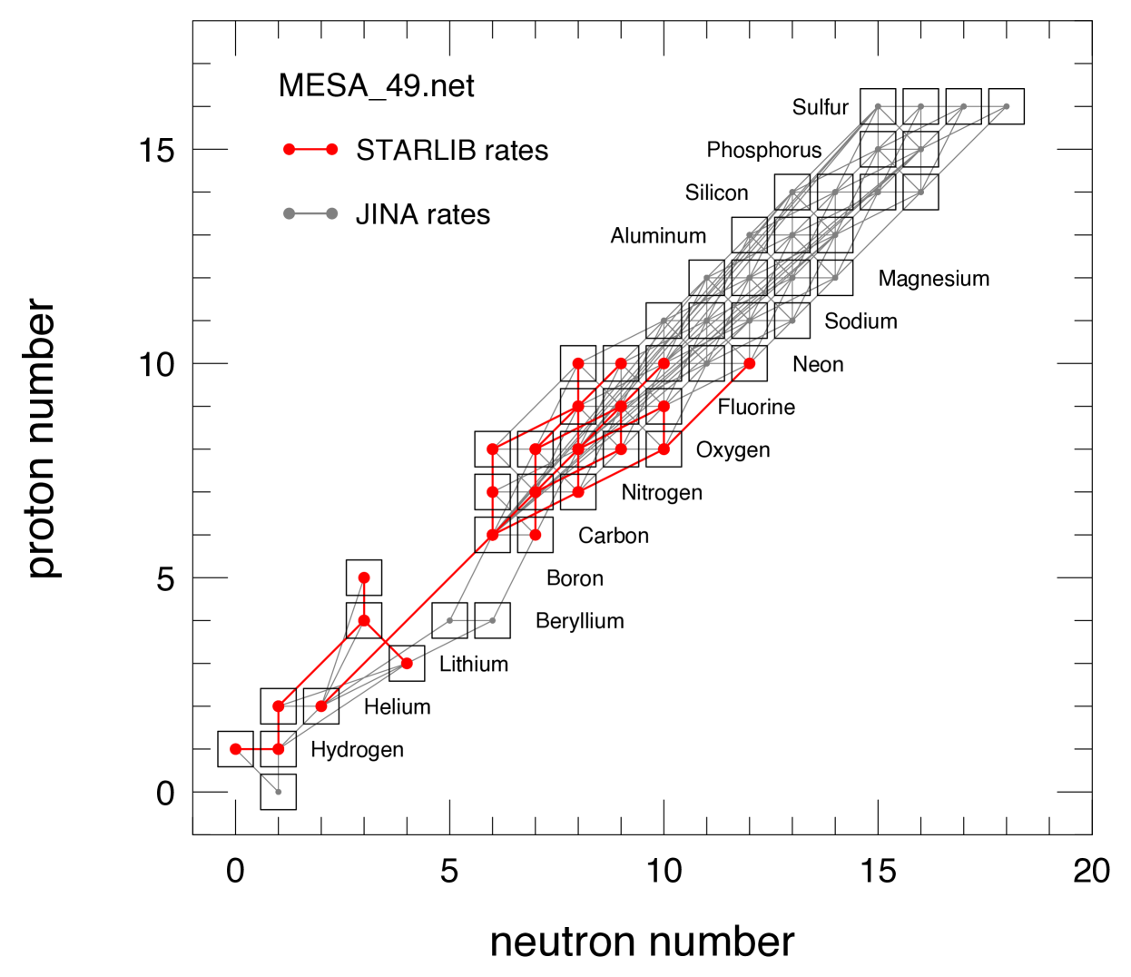
!htb Nuclear Reaction Reference Rate Identifier ¹H(p,$\gamma$)²H nacr (Exp.) 1 ²H(p,$\gamma$)³He de04 (Exp.) 2 ³He($\alpha$,$\gamma$)⁷Be cy08 (Exp.) 3 ⁷Li(p,n)⁷Be de04 (Exp.) 4 ⁷Be(p,$\gamma$)⁸B nacr (Exp.) 5 ¹²C(p,$\gamma$)¹³N nacr (Exp.) 6 ¹³C(p,$\gamma$)¹⁴N nacr (Exp.) 7 ¹³N(p,$\gamma$)¹⁴O nacr (Exp.) 8 ¹⁴N(p,$\gamma$)¹⁵O im05 (Exp.) 9 ¹⁵N(p,$\alpha$)¹²C nacr (Exp.) 10 ¹⁵N(p,$\gamma$)¹⁶O nacr (Exp.) 11 ¹⁴O($\alpha$,p)¹⁷F taly (Theory) 12 ¹⁵O($\alpha$,$\gamma$)¹⁹Ne mc10 (MC) 13 ¹⁶O(p,$\gamma$)¹⁷F mc10 (MC) 14 ¹⁷O(p,$\alpha$)¹⁴N bu15 (Exp.) 15 ¹⁷O(p,$\gamma$)¹⁸F bu15 (Exp.) 16 ¹⁸O(p,$\alpha$)¹⁵N mc13 (MC) 17 ¹⁸O(p,$\gamma$)¹⁹F mc13 (MC) 18 ¹⁷F(p,$\gamma$)¹⁸Ne mc10 (MC) 19 ¹⁸F(p,$\alpha$)¹⁵O mc10 (MC) 20 ¹⁹F(p,$\alpha$)¹⁶O nacr (Exp.) 21 ¹⁶O($\alpha$,$\gamma$)²⁰Ne mc10 (MC) 22 ¹⁴N($\alpha$,$\gamma$)¹⁸F mc10 (MC) 23 ¹⁸O($\alpha$,$\gamma$)²²Ne mc10 (MC) 24 ¹²C($\alpha$,$\gamma$)¹⁶O ku02 (Exp.) 25 Triple-$\alpha$ nacr (Exp.) 26

Table 1Sampled Nuclear Reaction Rates

Note. — Experimental reaction rates with approximate uncertainties are labeled ”Exp”, while experimental reaction rates with statistically rigorous uncertainties are labeled ”MC”. References are denoted as follows: nacr - Angulo et al. (1999), de04 - Descouvemont et al. (2004), cy08 - Cyburt & Davids (2008), im05 - Imbriani et al. (2005), taly - Sallaska et al. (2013), mc10 - Iliadis et al. (2010b), bu15 - Buckner et al. (2015), mc13 - Sallaska et al. (2013), and ku02 - Kunz et al. (2002). Rate identifiers (RI) in column 3 are assigned for later reference.

We evolve each stellar model with MESA’s mesa_49.net, a nuclear reaction network that follows 49 isotope from ¹H to ³⁴S. In Table 1, we list 26 forward nuclear reaction rates known to have an impact on the final state of the CO WD (Salaris et al., 1997; Metcalfe et al., 2002; Straniero et al., 2003). For detailed reviews on the structural and evolutionary properties of white dwarfs, see Koester (2002); Hansen & Liebert (2003); Althaus et al. (2010). For each stellar model, these 26 forward rates are sampled simultaneously and independently according to their experimental uncertainties. Otherwise, all forward thermonuclear reaction rates are from the JINA reaclib version V2.0 2013-04-02 (Cyburt et al., 2010a). We adopted this hybrid approach of using 26 Monte Carlo from STARLIB with the remaining rates from JINA reaclib because STARLIB is not yet fully integrated with MESA, requiring each STARLIB rate and uncertainty specification to be manually cast into MESA’s tabular format. The 405 reaction rates linking the 49 isotopes are shown in Figure 1.

Inverse rates are calculated directly from the forward rates (those with positive $Q$-value) using detailed balance, rather than using fitted rates. This is important for H and He burning processes approaching equilibrium (e.g., Hansen et al., 2004; Iliadis, 2007). The nuclear partition functions used to calculate the inverse rates are taken from Rauscher & Thielemann (2000). Thermal neutrino energy-losses are taken from the fitting formula of Itoh et al. (1996). Electron screening factors for both weak and strong thermonuclear reactions are taken from Alastuey & Jancovici (1978) with plasma parameters from Itoh et al. (1979). All the weak rates are based (in order of precedence) on the tabulations of Langanke & Martínez-Pinedo (2000), Oda et al. (1994), and Fuller et al. (1985).

3. Characteristics of the baseline 3 M_⊙ stellar model

In this section we present characteristics of the solar metallicity, non-rotating 3 M_⊙ model evolved with the STARLIB rates.

Figure 2.— Baseline 3 M_⊙ model with the nominal set of reaction rates in the HR diagram. Key events and ages are labeled.

Figure 3.— Kippenhahn diagram of the baseline 3 M_⊙ model from the MS to formation of a $\approx$ 0.645 M_⊙ WD.

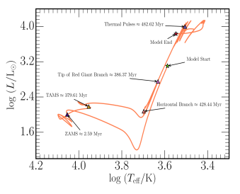
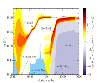
Figure 2 shows the model star in the HR diagram. Core H burning is initiated at $t\approx$ 2.59 Myr with a central pulse that lasts $t\approx$ 0.12 Myr while the star continues to contract from log($R/R_{\odot}$) $\approx$ 0.43 to 0.37. At $t\approx$ 3.26 Myr a subsequent H pulse halts further contraction and causes a decrease in the surface temperature and luminosity. This secondary pulse is quenched at $t\approx$ 3.48 Myr causing the star to expand to log($R/R_{\odot}$) $\approx$ 0.35. These unstable H pulses at the core of the stellar model cause the fluctuations near the labeled ZAMS location in Figure 2. Following the first two failed H pulses, burning in the core continues at $t\approx$ 3.80 Myr initiating a further contraction of the star from log($R/R_{\odot}$) $\approx$ 0.35 to 0.30. At this configuration, the stellar model proceeds through stable H burning until reaching the TAMS at $t\approx$ 379.6 Myr.

Once H is depleted in the core, the core contracts, the envelope expands, and the star ascends the RGB. The model star reaches log($R/R_{\odot}$) $\approx$ 1.65 at the tip of the RGB at an age of $t\approx$ 386.37 Myr. Helium burning begins in the core. The stellar model maintains core He burning while contracting to a radius of log($R/R_{\odot}$) $\approx$ 1.20. The star populates horizontal branch at an age of $t\approx$ 428.44 Myr. Once the supply of He fuel in the core is depleted, the star leaves the horizontal branch due to further core contraction and expansion of the envelope. The star ascends the AGB (e.g., Lattanzio, 1991; Iben, 1991; Karakas & Lattanzio, 2007; Shingles et al., 2015).

On the AGB, He burning continues in a thin shell above the newly formed CO core and the H burning shell. Figure 3 shows a Kippenhahn diagram of our 3 M_⊙ non-rotating stellar model. The color bar represents the net nuclear energy generation rate. Dark red-orange regions denote regions of strong nuclear burning such as the H and He burning shells annotated in the diagram. Regions of purple indicate a logarithmic increase in the cooling rate, such as in the CO core. Convective regions are shown in light blue. For simplicity, regions undergoing semi-convective, thermohaline, or convective boundary mixing are not shown.

Figure 4.— Helium burning luminosity during the thermal pulses relative to time at first thermal pulse at approximately 482.47 Myr.

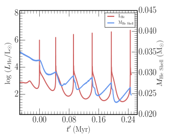
The geometrically thin He shell grows as material from H burning shell is processed, causing the He shell to increase in temperature and pressure. Once the mass in the He shell reaches a critical value, helium is reignited and causes a He shell flash. This flash causes an extraordinary release of energy and expansion of the intershell region. The first thermal pulse is achieved in our baseline model at an age of $t\approx$ 482.47 Myr. Figure 4 depicts the subsequent thermal pulses by showing He burning luminosity as a function of stellar age. The time between pulse is often referred to as the interpulse period and has been shown to be well described by

$$\textup{log}~{}\Delta t_{\rm{TP}}=4.5(1.689-M_{\rm{CO}})~{}\rm{yr}$$ (1)

for $Z$ = 0.02 (Boothroyd & Sackmann, 1988).

Our solar metallicity 3 M_⊙ model goes through a series of six thermal pulses, $n_{\rm{TP}}=6$, with a recurrence time of log($\Delta t_{\rm{TP}}/{\rm yr})\approx$ 4.66. This value agrees to within a factor of two of Equation (1). The difference is due to the He abundance used in our model, $Y=0.28$, and the strong dependence of Equation (1) on the He abundance (Boothroyd & Sackmann, 1988).

The luminosity of a Red Supergiant with a degenerate CO core and H and He shell sources may be approximated by the core mass - luminosity relationship

$$\begin{split}L/L_{\odot}=&\ 2.38\times 10^{5}\mu^{3}Z^{0.04}\\ &\times(M_{\rm{CO}}^{2}-0.0305M_{\rm{CO}}-0.1802)\end{split}$$ (2)

for core masses 0.5 M_⊙ $\lesssim$ $M_{\rm{CO}}$ $\lesssim$ 0.66 M_⊙ (Marigo et al., 1996, 1998). At the peak luminosity of the final thermal pulse our stellar model reaches log($L/L_{\odot}$) $\approx$ 4.14. This value agrees to within $\approx$ 5% using Equation (2) with $\mu\approx$ 0.621, $Z$=0.02, and $M_{\rm{CO}}\approx$ 0.585 M_⊙.

Figure 5.— Density and abundance profiles in the 0.64 M_⊙ CO WD remnant produced by the 3 M_⊙ model. The MESA density structure (dashed purple curve) is compared to polytropic density profiles for $n$ = 3/2, 2, 5/2, 3, and 7/2.

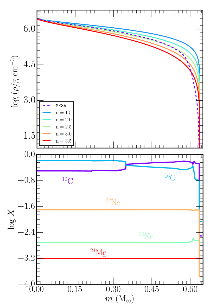
Figure 5 shows the density and abundance profiles of the CO WD remnant. The upper panel shows the density profile of the MESA model (dashed line) and polytropic density of varying indices $n$. For the nearly isothermal core temperature of $T\approx 1\times 10^{8}$ K, the MESA density profile is best fitted by a density profile of a $n$=5/2 polytrope.

In the baseline 3 M_⊙ model, ⁴He initially burns to ¹²C via the triple-$\alpha$ reaction in the core on a timescale of $\approx$ 50 Myr. Once an abundance of carbon builds up, ¹²C can capture an alpha particle to become ¹⁶O. For the 3 M_⊙ model, this occurs on longer timescales of $\approx$ 100 Myr (e.g., Iben, 2013a, b). Late in core He burning, the rising abundance of ¹²C allows alpha capture to compete with and eventually dominate the triple-$\alpha$ flow, which thus causes the ¹²C to decrease. By the end of core He burning the mass fractions are X(_c¹²C) = 0.3151 and X_c(¹⁶O) = 0.6585. The remaining $\approx$ 2.6% of the original He is mostly in isotopes of Ne and Mg.

Figure 6.— Mass of the CO core (purple), age (blue-green), central temperature $T_{\mathrm{\!c}}$ (gold), and central density $\rho_{\mathrm{c}}$ (red) at the first thermal pulse, normalized to the values from our baseline choice of ($\delta_{\rm{mesh}}$ =0.5,$w_{\rm{t}}$ =10^-4). The other spatial and temporal combinations shown are ($\delta_{\rm{mesh}}$ =1.0,$w_{\rm{t}}$ =10^-2), ($\delta_{\rm{mesh}}$ =0.75,$w_{\rm{t}}$ =10^-3), and ($\delta_{\rm{mesh}}$ =0.25,$w_{\rm{t}}$ =10^-5).

The isotope ²²Ne is perhaps the most interesting of these remaining isotopes as it carries all of the available neutrons, which can have significant consequences on the peak luminosity of any subsequent explosion of the CO WD as a supernova Type Ia (e.g., Townsley et al., 2009; Howell et al., 2009; Neill et al., 2009; Childress et al., 2013; Moreno-Raya et al., 2015). Most of a main-sequence star’s initial metallicity $Z$ comes from the CNO and ⁵⁶Fe nuclei inherited from its ambient interstellar medium. The slowest step in the hydrogen burning CNO cycle is proton capture onto ¹⁴N. This results in all the CNO catalysts piling up into ¹⁴N when hydrogen burning on the main sequence is completed. During He burning the reactions ${}^{14}{\rm N}(\alpha,\gamma)^{18}{\rm F}(,\beta^{+}\nu_{e})^{18}{\rm O}(\alpha,\gamma)^{22}{\rm Ne}$ convert all of the ¹⁴N into ²²Ne. Thus, the final mass fraction of ²²Ne in the CO remnant

$$X(^{22}{\rm Ne})=22\left(\frac{X(^{12}{\rm C})}{12}+\frac{X(^{14}{\rm N})}{14}+\frac{X(^{16}{\rm O})}{16}\right)$$ (3)

is determined by the birth abundances of CNO. For the solar mass fractions used in constructing the initial 3 M_⊙ model, Equation (3) gives ${\rm X}(^{22}{\rm Ne})$=0.021 gives the same value shown in Figure 5. In Figure 5 we also see a notable feature at the chemical transition region from ¹⁶O to ¹²C. These transition regions were found to be caused by extra mixing episodes during core He burning and have implications for the Brunt-V$\ddot{\rm{a}}$is$\ddot{\rm{a}}$l$\ddot{\rm{a}}$ frequency profile (Romero et al., 2012, 2013).

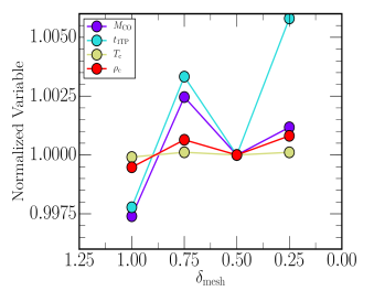
To assess the convergence of our 3 M_⊙ model to the choice of spacetime resolution parameters we evolve a series of models from the pre-MS to the first thermal pulse and varying the spatial resolution parameter mesh_delta_coeff, $\delta_{\rm{mesh}}$, and temporal resolution parameter varcontrol_target, $w_{\rm{t}}$. The spatial and temporal resolutions explored are ($\delta_{\rm{mesh}}$ =1.0,$w_{\rm{t}}$ =10^-2), ($\delta_{\rm{mesh}}$ =0.75,$w_{\rm{t}}$ =10^-3), ($\delta_{\rm{mesh}}$ =0.5,$w_{\rm{t}}$ =10^-4), and ($\delta_{\rm{mesh}}$ =0.25,$w_{\rm{t}}$ =10^-5). Changing $\delta_{\rm{mesh}}$ by a factor of two, changes the number of cells by roughly a factor of two, and changing $w_{\rm{t}}$ by a factor of ten changes the timestep by a factor of roughly two.

Figure 6 shows the mass of the CO core, age, $T_{\mathrm{\!c}}$, and $\rho_{\mathrm{c}}$ at the first thermal pulse. Each of these quantities is normalized to the values from our baseline choice of ($\delta_{\rm{mesh}}$ =0.5,$w_{\rm{t}}$ =10^-4). Figure 6 suggests these key end-of-evolution quantities are converged with regard to the mass grid and timestep to within 3 to 4 significant figures.

4. Reaction Rate Sampling

Figure 7.— The ¹²C$(\alpha,\gamma)^{16}$O nuclear reaction rate, normalized by the rate given in JINA-REACLIB, for Caughlan & Fowler (1988, CF88), Angulo et al. (1999, NACR), Cyburt et al. (2010b, JINA-REACLIB), Sallaska et al. (2013, STARLIB Median), and a sampled rate distribution (STARLIB Sampled) computed for a specific Gaussian deviate of $p_{i}$ = 0.849741. The JINA-REACLIB rate is based on Buchmann (1996) and STARLIB on Kunz et al. (2002). Note: The CF88 rate used in MESA is 1.7 times the original CF88, see Weaver & Woosley (1993).

The STARLIB rate library provides the median nuclear reaction rate, $\textup{Rate}_{\rm{med}}$, and the associated factor uncertainty, henceforth $f.u.$, at temperature ranges from $10^{6}$ K to $10^{10}$ K (Sallaska et al., 2013). Following Longland et al. (2010), all reaction and decay rates given in STARLIB are assumed to follow a log-normal probability distribution. Such a distribution is described by the location and spread parameters, $\mu$ and $\sigma$, respectively. These parameters can be obtained using the median rate and $f.u.$ tabulated in STARLIB, where $\sigma=\textup{ln}~{}f.u.$, $\mu=\textup{ln}~{}\textup{Rate}_{\rm{med}}$. These two parameters give a complete description of the reaction rate probability density at any temperature.

The relationship between these parameters form the basis of our sampling scheme. Following Evans et al. (2000), for a log-normal distribution of an arbitrary quantity, $x$, samples are drawn as,

$$x_{i}=e^{\mu+\sigma p_{i}}\equiv e^{\mu}(e^{\sigma})^{p_{i}}~{}.$$ (4)

Using the relations for $\mu$ and $\sigma$, we can obtain a sampled rate distribution as a function of temperature from

$$\textup{Rate}_{\rm{samp}}=e^{\mu}(e^{\sigma})^{p_{i,j}}=\textup{Rate}_{\rm{med}}(f.u.)^{p_{i,j}}~{},$$ (5)

where $p_{i,j}$ is standard Gaussian deviate with mean of zero and standard deviation of unity for the $j$th sampled reaction rate.

We refer to $p_{i,j}$ as the rate variation factor for the $j$th reaction, following the $j$ rate identifiers given in Table 1. The rate variation factor $p_{i,j}$ differs from the factor uncertainty $f.u.$. For a rate variation factor of $p_{i,j}$=0, the median Monte Carlo rate provided by STARLIB is recovered. Since the factor uncertainty $f.u.$ is a function of temperature, a sampled rate distribution follows the temperature dependence of the uncertainty in the rate.

In this study, we independently sample 26 forward thermonuclear reaction rates (see Table 1) that describe the main H and He burning processes relevant to the evolution and subsequent formation of CO WDs. Because MESA calculates inverse rates directly from the forward rates (those with positive $Q$-value) using detailed balance, we also implicitly, but not independently, sample the corresponding 26 inverse rates.

Figure 8.— The factor uncertainty, f.u., for the triple-$\alpha$, ¹²C($\alpha$,$\gamma$)¹⁶O, ¹⁶O($\alpha$,$\gamma$)²⁰Ne, and ¹⁴N($p$,$\gamma$)¹⁵O reaction rates over stellar H and He burning temperatures. STARLIB data points are shown by the filled dots, while the lines represent interpolations of the data.

Experimentally-based Monte Carlo reaction rate distributions are available for 9 out of 26 of the reactions rates included in our sampling scheme. For 16 reactions, such as ${}^{12}\textup{C}(\alpha,\gamma)\rm{{}^{16}O}$ and ${}^{14}\textup{N}(p,\gamma)\rm{{}^{15}O}$, Monte Carlo based rate distributions do not yet exist. This is due in part to these reaction rates being determined by broad amplitudes rather than narrow resonances. For such reactions, median rate values and $f.u.$ are obtained from estimates of experimental uncertainty where available. In the absence of experimental nuclear physics input, such as the ${}^{14}\textup{O}(\alpha,p)\rm{{}^{17}F}$ reaction, theoretical median rate values are obtained using the statistical (Hauser-Feshbach) model of nuclear reactions and computed using the nuclear reaction software instrument TALYS (Goriely et al., 2008).

Following Iliadis et al. (2015), we assume that the deviate is independent of temperature, $p_{i}(T)=$ constant. This simplification was shown to reproduce the same uncertainties in isotopic abundances as more complex sampling schemes (Longland, 2012). Despite this assumption for our rate variation factors, the $f.u.$ provided by STARLIB is temperature dependent. This allows us to closely follow changes in the rate uncertainty that have been shown to occur from different resonance contributions.

To initialize a grid of Monte Carlo stellar models we generate 26 independent random Gaussian distributions of rate variation factors, $p_{i,j}$, where $j$ corresponds to the rate identifiers listed in Table 1. A set of N stellar models is then constructed by using the $n^{\rm{th}}$ set of random numbers, the $p_{i,j}$, and Equation (5) to generate sampled reaction rate distributions.

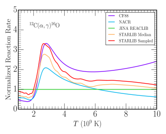
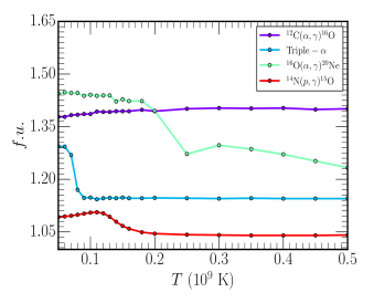
Once these 26 independently sampled STARLIB rate distributions are constructed, they are provided in tabular form to MESA. The data are used by MESA to perform an interpolation over a reaction rate defined by 10,000 points. Figure 7 shows a comparison of a sampled reaction rate distribution for the ¹²C$(\alpha,\gamma)^{16}$O reaction with $p_{i}$ = 0.849741 to fixed reaction rates from previous studies. Figure 8 plots the $f.u.$ for the the triple-$\alpha$, ¹²C($\alpha$,$\gamma$)¹⁶O, ¹⁶O($\alpha$,$\gamma$)²⁰Ne, and ¹⁴N($p$,$\gamma$)¹⁵O reaction rates over H and He burning temperatures. In broad terms, $f.u.$ represents the amount a reaction rate is shifted relative to the median reaction rate at each temperature.

5. Monte Carlo Stellar Models

Figure 9.— Histograms of the 1,000 3 M_⊙ Monte Carlo stellar model grid sampling 26 STARLIB reaction rates. Global and core properties shown include the mass of the CO core (A), age (B), central temperature (C), central density (D), central electron fraction (E), central ²²Ne mass fraction (F), central ¹²C mass fraction (G), and central ¹⁶O mass fraction (H), all at first thermal pulse. The green dashed lines and the dot dashed red lines denote the 68% and 95% confidence intervals, respectively. The mean values for the eight quantities shown here, are enumerated in Table 2.

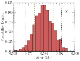
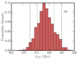
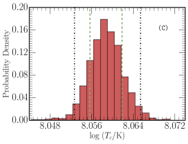
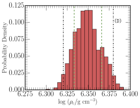
We evolve 1,000 3 M_⊙ models from the pre-MS to the first thermal pulse (1TP), with each model using a different set of sampled nuclear reaction rates from STARLIB. MESA defines the 1TP as the evolutionary point at which the central He mass fraction, X${}_{\rm c}(^{4}\rm{He})$, is depleted, the He shell mass is $\leq$ 0.2 M_⊙, and their is presence of a convective zone with helium burning. Once a 3 M_⊙ model has reached this evolutionary point, the newly formed convective core is composed primarily of CO. Evolution to this key event allows a robust grid of 1,000 stellar models to be computationally feasible; each stellar model in the grid took $\approx$ 24 core-hours to reach the 1TP. Additionally, stopping the stellar model at the 1TP allows an unbiased means to identify critical reaction rates in the H and He burning processes leading to the formation of a CO WD. For a Gaussian distribution with standard deviation of unity, we expect a standard error of $\sigma/\sqrt{1000}\approx 3\%$ for each independently sampled reaction rate.

!htb Variable Mean 68% C.I. 95% C.I. % Change $M_{\rm{1TP}}$ (M_⊙) 5.838(-1) 9.582(-3) 1.884(-2) 3.227 $t_{\rm{1TP}}$ (Myr) 4.786(2) 6.611 1.250(1) 2.612 log($T_{{\rm c}}/{\rm K})$ 8.059 6.164(-3) 1.269(-2) 0.157 log($\rho_{{\rm c}}/{\rm g\ cm}^{-3}$) 6.349 3.252(-2) 5.938(-2) 0.935 $Y_{\rm{e,c}}$ 4.990(-1) 1.277(-5) 2.557(-5) 0.005 X${}_{\rm{c}}(^{22}$Ne) 1.997(-2) 2.898(-4) 5.812(-4) 2.910 X${}_{\rm{c}}(^{12}$C) 3.365(-1) 2.076(-1) 3.916(-1) 116.4 X${}_{\rm{c}}(^{16}$O) 6.372(-1) 2.076(-1) 3.920(-1) 61.52

Table 2Variations in core quantities

Note. — The ($n$) after a given value, A, denotes A $\times$ 10ⁿ.

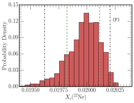
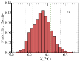
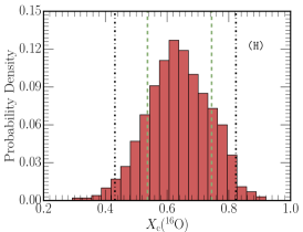
Figure 9 shows histograms of $M_{\rm{1TP}}$ (A), $t_{{\rm 1TP}}$ (B), $T_{\mathrm{\!c}}$(C), $\rho_{\mathrm{c}}$ (D), $Y_{\rm e,c}$ (E), X_c(²²Ne) (F), X_c(¹²C) (G), and X_c(¹⁶O) (H), all at the 1TP. The number of bins is chosen according to the Rice Rule, $k=[2n^{1/3}]$, where $k$ is the number of bins and $n$ is the number of data points (Lane, 2013). The green dashed lines and the dot dashed black lines denote the 68% and 95% confidence intervals (C.I.), respectively. Relative to the arithmetic mean value, we find the width of the 95% confidence interval to be $\Delta M_{{\rm 1TP}}$ $\approx$ 0.019 M_⊙ for the core mass at the 1TP, $\Delta$$t_{\rm{1TP}}$ $\approx$ 12.50 Myr for the age, $\Delta\log(T_{{\rm c}}/{\rm K})\approx$ 0.013 for the central temperature, $\Delta\log(\rho_{{\rm c}}/{\rm g\ cm}^{-3})\approx$ 0.060 for the central density, $\Delta Y_{\rm{e,c}}\approx$ 2.6$\times$10^-5 for the central electron fraction, $\Delta X_{\rm{c}}(^{22}\rm{Ne})\approx$ 5.8$\times$10^-4, $\Delta X_{\rm{c}}(^{12}\rm{C})\approx$ 0.392, and $\Delta X_{\rm{c}}(^{16}\rm{O})\approx$ 0.392. In Table 2 we compile the arithmetic mean values of the eight quantities shown in Figure 9, the width of the 68% and 95% confidence intervals, and the percentage change from the arithmetic mean using the 95% confidence interval. To find the main sources of these global variations we use a Principal Component Analysis and Spearman Rank-Order Correlation.

5.1. Principal Component Analysis

Figure 10.— PCA correlation matrix for the 26 STARLIB reaction rates and 8 quantities of the CO remnant for the 1,000 MC 3 M_⊙ stellar models. Labeled are the reaction rates whose experimental uncertainties show a significant correlation with the 8 quantities measured at the 1TP. The colored box to the left to a vertical line is the labeled quantity.

Principal Component Analysis (PCA) is a statistical method used to transform a set of possibly correlated observations to a set linearly uncorrelated variables, referred to as principal components (Jolliffe, 2002; Jackson, 2005). Among numerous applications, a PCA has been used to analyze large scale spectra of the Interstellar Medium (Heyer & Schloerb, 1997), to classify optical stellar spectra of O to M type stars (Singh et al., 1998), and investigate the far infrared spectral density of simulated galaxies (Safarzadeh et al., 2016). Our goal with a PCA is to determine which reaction rate uncertainties account for most of the global variability in the 3 M_⊙ MC stellar evolution models. We consider 34 quantities in total $-$ the 26 STARLIB reaction rate variation factors in the order listed in Table 1, $M_{{\rm 1TP}}$, $t_{\rm 1TP}$, $T_{\rm{c}}$, $\rho_{\mathrm{c}}$, $Y_{\rm e,c}$, X_c(¹²C), X_c(¹⁶O), and X_c(²²Ne) all at the 1TP.

We use the Python NumPy module corrcoef (Walt et al., 2011) to calculate the 34x34 correlation matrix ${\bf C}$ of the 34x1000 data matrix ${\bf A}$, where the correlation matrix is related to the covariance matrix ${\bf Cov}$ by ${\bf C}_{ij}={\bf Cov}_{ij}/(\sigma_{i}\sigma_{j})$ where $\sigma_{i}$ and $\sigma_{j}$ are the standard deviations. Figure 10 shows the symmetric correlation matrix. Reaction rate uncertainties which show a significant correlation (red) or anti-correlation (blue) are labeled along with the 8 quantities of the CO remnant at the 1TP. Most of the lower left part of the correlation matrix shows no correlation showing the reaction rates are generally independent of each other. We note here that $M_{{\rm 1TP}}$ and $t_{\rm 1TP}$ are correlated with ¹²C($\alpha$,$\gamma$), $\rho_{\mathrm{c}}$, and X_c(¹⁶O) while being anti-correlated with 3$\alpha$ $T_{\rm{c}}$, and X_c(¹²C). The stellar age $t_{\rm 1TP}$ is correlated with the slowest reaction rate of the CNO-cycle ¹⁴N($p,\gamma$), and $Y_{e}$ is correlated with ¹⁴N($p,\gamma$), ¹⁵N($p,\alpha$), ¹⁵N($p,\gamma$), and to a lesser extent ¹⁶O($p,\gamma$). In addition $T_{\rm{c}}$ and $\rho_{\mathrm{c}}$ are anti-correlated as is $Y_{\rm{e}}$ and X_c(²²Ne). We defer a more detailed physical interpretation of these trends to §5.3.

b Component Eigenvalue Proportion Cumulative 1 5.5917 0.1645 0.1645 2 3.0743 0.0904 0.2549 3 1.6734 0.0492 0.3041 4 1.2910 0.0380 0.3421 5 1.2502 0.0368 0.3789

Table 3Principal Component Analysis

We use the Python NumPy module, linalg.eig (Walt et al., 2011), to calculate the eigenvectors and eigenvalues of the correlation matrix shown in Figure 10. A principal component is constructed using the eigenvector coefficients of a given eigenvalue. The first principal component takes the form,

$$Y_{\rm{1}}=e_{1,1}X_{1}+e_{1,2}X_{2}+\ldots e_{1,34}X_{34}~{},$$ (6)

where $X_{1}$ is the first row in the data matrix A, and $e_{\rm{i,j}}$ is the coefficient of the eigenvector for the $i^{\rm{th}}$ principal component and $j^{\rm{th}}$ quantity. The proportion of variation explained by the $i^{\rm{th}}$ principal component can be characterized by the ratio $i^{\rm{th}}$ eigenvalue to that of the summation of all eigenvalues. In Table 3 we show the eigenvalues, proportion of total variation, and cumulative proportion of total variation for the first five principal components of our correlation matrix, ${\bf C}$. The first five components account for $\approx$ 38% of the total variation with only $\approx$ 16% accounted for by the first component.

To determine which quantities have the most impact on the total variation we consider the relative contributions of each coefficient. The largest coefficient in the first principal component, with a value of +0.517, corresponds to $T_{\mathrm{\!c}}$. The two subsequent coefficients that are largest in magnitude are (-0.428, -0.404), corresponding to X_c(¹²C) and X_c(¹⁶O), respectively. Next, we consider the effect of the sampled reaction rates in individual physical quantities using the method of Spearman Rank-Order Correlation.

5.2. Spearman Rank-Order Correlation

Figure 11.— Spearman rank correlation coefficients for the 26 independently sampled nuclear reaction rates for 1,000 Monte Carlo stellar models with a ZAMS mass of 3 M_⊙. The rate identifiers correspond to those listed in Table 1. Each sampled rate is compared individually against the final mass of the CO core ($M_{{\rm 1TP}}$, A), age of stellar model ($t_{{\rm 1TP}}$, B), central temperature ($T_{{\rm c}}$, C), central density ($\rho_{{\rm c}}$, D), central electron fraction ($Y_{{\rm e,c}}$, E), central neon 22 mass fraction (X_c(²²Ne), F), central ¹²C mass fraction (X_c(¹²C), G), and central ¹⁶O mass fraction (X_c(¹⁶O), H) at the 1TP.

Spearman Rank-Order Correlation determines if there is a monotonically increasing or decreasing relationship between two scalar quantities. The Spearman correlation coefficient, $r_{\rm{s}}$, is defined as the Pearson’s correlation coefficient between ranked variables. For a sample size $N$, the data are converted to ranks and $r_{\rm{s}}$ is computed as,

$$r_{\mathrm{s}}=1-\frac{6}{N(N^{2}-1)}\sum\limits_{i=1}^{N}d_{\rm{i}}^{2}~{},$$ (7)

where $d_{\rm{i}}$ is the difference between the ranks of two scalar quantities. A value of $r_{\mathrm{s}}$= +1 would represent a perfectly monotonically increasing relationship, $r_{\mathrm{s}}$= 0, perfectly uncorrelated, and $r_{\mathrm{s}}$=-1, monotonically decreasing.

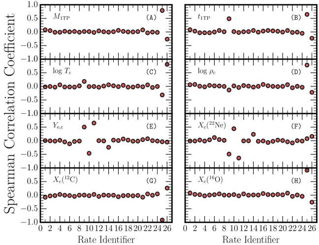
In Figure 11, we show the Spearman coefficients against the 26 independently sampled rate variation factors for $M_{{\rm 1TP}}$ (A), $t_{{\rm 1TP}}$ (B), $T_{{\rm c}}$ (C), $\rho_{{\rm c}}$ (D), $Y_{{\rm e,c}}$ (E), X_c(²²Ne) (F), X_c(¹²C) (G), and X_c(¹⁶O) (H) at the 1TP.

The uncertainties in the nuclear reaction rates that have the largest effect on $M_{{\rm 1TP}}$ are ${}^{12}\textup{C}(\alpha,\gamma)$ with $r_{\mathrm{s}}$=+0.79 and triple-$\alpha$ with $r_{\mathrm{s}}$=-0.26. The uncertainties in the remaining rates have a negligible effect on $M_{{\rm 1TP}}$, $-0.03\lesssim r_{\mathrm{s}}\lesssim+0.08$. The same uncertainties in the reaction rates have the largest impact on the stellar age. However, the reaction ${}^{14}\textup{N}(p,\gamma)$ also plays a significant role with $r_{\mathrm{s}}$=+0.49. For $T_{\rm{c}}$ the uncertainties in the rates that show the largest coefficients are ${}^{12}\textup{C}(\alpha,\gamma)$ with $r_{\mathrm{s}}$=-0.32, triple-$\alpha$ with $r_{\mathrm{s}}$=+0.81, and ¹⁴N(p,$\gamma$) with $r_{\mathrm{s}}$=+0.18. For $\rho_{\mathrm{c}}$, the same uncertainties in the reaction rates dominate with $r_{\mathrm{s}}$=(+0.78, -0.22, -0.13), respectively. The largest coefficients for $Y_{\rm{e,c}}$ correspond to the uncertainties in ¹⁴N(p,$\gamma$) with $r_{\mathrm{s}}$=+0.50, ¹⁵N(p,$\alpha$) with $r_{\mathrm{s}}$=-0.46, and ¹⁵N(p,$\gamma$) with $r_{\mathrm{s}}$=+0.65. Similarly, variations in X_c(²²Ne) depend mostly on the uncertainties in the same three reactions, where we find $r_{\mathrm{s}}$=(-0.49, +0.44, -0.64) respectively. Related, X_c(${}^{12}\textup{C})$ and X_c(${}^{16}\textup{O}$) are dominated only by ${}^{12}\textup{C}(\alpha,\gamma)\rm{{}^{16}O}$ and triple-$\alpha$. For X_c(¹²C), the coefficients are $r_{\mathrm{s}}$=(-0.91, +0.26) respectively, while for X_c(¹²O) we find $r_{\mathrm{s}}$=(+0.91, -0.26) respectively. These trends in the Spearman coefficients verify the PCA results of §5.1.

5.3. Properties of Carbon-Oxygen White Dwarfs

Here we discuss the individual nuclear reaction rates which have been identified to have the most significant impact on the WD composition and structural properties. In the previous section we identified ¹⁴N(p,$\gamma$), ¹⁵N(p,$\alpha$), ¹⁵N(p,$\gamma$), triple-$\alpha$, and ${}^{12}\textup{C}(\alpha,\gamma)$ as having the largest impact on the physical properties of the WD.

5.3.1 ¹⁴N(p,$\gamma$)¹⁵O

The ¹⁴N($p,\gamma$)¹⁵O was identified as having a significant impact on the age, $T_{\mathrm{\!c}}$, $Y_{\rm e,c}$ , and X_c(²²Ne). As noted previously in §3 and §5.1, this reaction is the slowest reaction in the CNO cycle. This result was confirmed in the seminal first direct measurements at astrophysical energies (LUNA Collaboration et al., 2006).

In Figure 12 we show the stellar age versus the effective rate variation factor. Each of the 1,000 3 M_⊙ MC stellar models is a data point in the figure. Also shown are the 1$\sigma$ (68%, red), 2$\sigma$ (95%, green) and 3$\sigma$ (99.7%, blue) deviations about the mean. Orientation of the uncertainty ellipsoid is determined by the unit eigenvectors of the 2x2 covariance matrix, and the lengths of the semi-major and semi-minor axes of the ellipsoid correspond to the positive square roots of the two eigenvalues.

To quantify how well the rate variation factor can account for the increase in age, we perform a linear regression analysis. The coefficient of determination ($R^{2}$ value) is the squared Pearson product-moment correlation coefficient. For two quantities with a perfectly linear relationship, $R^{2}$=1. The lower the $R^{2}$ value, the less that the corresponding linear fit can account for the data. For perfectly uncorrelated data, an $R^{2}$=0. For the stellar age data, the regression analysis yields $R^{2}$=0.257. This suggests that although we find a relatively large Spearman coefficient for the rate variation factor and the age, other rates play a significant factor in this quantity as well.

Figure 12.— Rate variation factor for ¹⁴N($p,\gamma$)¹⁵O versus stellar age at the 1TP, see Equation (5). Each of the 1,000 Monte Carlo 3 M_⊙ models produces a data point in the figure. Overlaying the data points are the 1$\sigma$ (68%, red), 2$\sigma$ (95%, green) and 3$\sigma$ (99.7%, blue) deviations about the mean of the data points. A linear regression is performed on the raw data (gold solid line), yielding an $R^{2}$=0.257.

Figure 13.— Same as in Figure 12 but for ¹⁵N($p,\alpha$)¹²C versus X_c(²²Ne) at the 1TP. The linear regression yields $R^{2}$ = 0.207.

Figure 14.— Same as in Figure 13 but for triple-$\alpha$ versus $T_{\rm{c}}$. The linear regression performed yields an $R^{2}$=0.680.

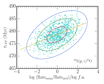
The first principal component can be represented by the line, the major axis of the uncertainty ellipse, which minimizes the summed squared distance of closest approach, i.e. the distance perpendicular to the major axis line. Linear least squares regression minimizes the summed square distance in the one direction only. Thus, although the two methods use a similar error metric, linear least squares treats one dimension of the data preferentially, while PCA treats all dimensions equally. Hence the major axis in Figure 12 is not aligned with the least squares regression line.

For $T_{\rm{c}}$, $Y_{\rm{e,c}}$, and X_c(²²Ne) we find $R^{2}$=0.017, 0.246, and 0.239, respectively. The central $Y_{\rm e,c}$ and X_c(²²Ne) are anti-correlated because X_c(²²Ne) largely determines $Y_{\rm e,c}$

$$Y_{\rm e,c}=\frac{1}{2}-\frac{X_{\rm c}(^{22}{\rm Ne})}{22}\ ~{}.$$ (8)

An increase in X_c(²²Ne) decrease $Y_{e}$, accounting for the similar magnitudes of $R^{2}$.

5.3.2 ¹⁵N(p,$\alpha$)¹²C

Formed from the ¹⁴N(p,$\gamma$)¹⁵O reaction, ¹⁵O has a half-life of $\tau_{1/2}\approx$122 seconds undergoing beta decay to form ¹⁵N. The creation of ¹⁵N signals the end of the catalytic CNO cycle to form ⁴He and ¹²C. We previously identified the ¹⁵N(p,$\alpha$)¹²C reaction as having a significant impact on $Y_{\rm e,c}$ and X_c(²²Ne) - see Equation (8).

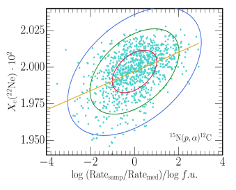
Figure 13 shows the rate variation factor for the ¹⁵N(p,$\alpha$)¹²C reaction versus the scaled X_c(²²Ne). The ellipsoid width suggests the uncertainties from multiple reactions impact X_c(²²Ne). The regression fit gives $R^{2}$ = 0.207. For 3$\sigma$ changes in the ¹⁵N(p,$\alpha$)¹²C rate variation factor, only small changes in X_c(²²Ne) are induced, with $\Delta$X_c(²²Ne)$\approx\pm 4\times 10^{-4}$ and $\Delta Y_{\rm{e}}\approx\pm 4\times 10^{-4}$.

5.3.3 ¹⁵N(p,$\gamma$)¹⁶O

The central $Y_{\rm e,c}$ and X_c(²²Ne) pair depends on the efficiency of the ¹⁵N(p,$\gamma$)¹⁶O reaction. In §3, X_c(²²Ne) was shown to be well approximated by Equation (3). The Spearman correlation coefficient between the rate variation factor for ¹⁵N(p,$\gamma$)¹⁶O and X_c(²²Ne) suggested that for a decrease in rate efficiency, there would be a decrease in X_c(²²Ne). This is confirmed through Equation (3). As a result, we have a larger $Y_{\rm e,c}$, as suggested by Figure 11.

5.3.4 Triple-$\alpha$

The triple-$\alpha$ reaction is one of the key nuclear reactions for the synthesis of the elements and is the main energy source during He burning. The reaction rate is dominated by resonances, the best known being the Hoyle state at 7.65 MeV (Hoyle, 1954), but there remains considerable interest in determining all resonances with high precision (Chernykh et al., 2010). The triple-$\alpha$ rate directly affects $M_{{\rm 1TP}}$, $t_{{\rm 1TP}}$, $T_{\mathrm{\!c}}$, $\rho_{\mathrm{c}}$, X_c(¹²C) and X_c(¹⁶O).

Triple-$\alpha$ rate variation factors of $\approx$ 1, 2, and 3 produce variations of $\approx$ 0.008, 0.0192, and 0.03 M_⊙ in the mass of the CO remnant. Increasing the triple-$\alpha$ rate generally leads to smaller CO core masses. This is largely due to larger triple-$\alpha$ rates depleting He fuel faster during shell He burning, leading to thinner He shell masses with shorter shell He lifetimes and thus less massive CO cores (see Figure 3). For the stellar age, the mean trend is for larger triple-$\alpha$ rates to produce shorter evolutionary times from the pre-MS to the 1TP, due to larger triple-$\alpha$ rates depleting the available core He fuel faster. A rate variation factor between -2.0 and 2.0 produces a $\approx$ 12 Myr change in the evolutionary time to reach the 1TP relative to the 478 Myr using the median reaction rate in our 3 M_⊙ model. For the triple-$\alpha$ rate versus $M_{{\rm 1TP}}$ and $t_{{\rm 1TP}}$, we find $R^{2}$=0.080 and 0.060, respectively. While the Spearman correlation coefficients obtained suggested a monotonically decreasing relationship for these two quantities, the majority of the variation cannot be accounted for by the triple-$\alpha$ reaction.

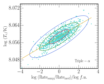
Figure 14 shows the strongly correlated relation between $T_{\rm{c}}$ at the 1TP and the triple-$\alpha$ rate. Larger rates tend to produce larger $T_{\rm{c}}$, although the magnitude of the effect is relatively small, with a rate variation factor between -3.0 and 3.0 (corresponding to the extrema loci of the 3$\sigma$ ellipse), producing a $\approx$ 5.5$\times$10⁶ K change in $T_{\rm{c}}$.

The central density $\rho_{\mathrm{c}}$ at the 1TP is less correlated with triple-$\alpha$ rate than $T_{\rm{c}}$. Larger rates tend to yield smaller $\rho_{\mathrm{c}}$. A rate variation factor between -3.0 and 3.0 produces a $\approx$ 5.1$\times$10⁵ g cm^-3 change in $\rho_{\mathrm{c}}$, a 23% difference.

Figure 15.— Same as in Figure 14 but for triple-$\alpha$ versus X_c(¹²C). The linear regression yields $R^{2}$ = 0.072.

Figure 16.— Same as in Figure 15 but for ¹²C($\alpha$,$\gamma$)¹⁶O versus $\rho_{\mathrm{c}}$ at the 1TP. The linear regression yields $R^{2}$ = 0.618.

Figure 17.— Same as in Figure 16 but for ¹²C($\alpha$,$\gamma$)¹⁶O versus X_c(¹²C0 at the 1TP. The linear regression yields $R^{2}$ = 0.854.

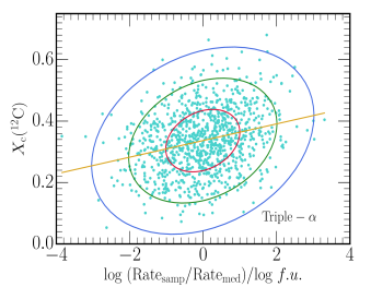
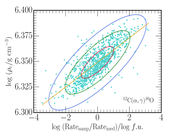
The central X_c(¹²C) and X_c(¹⁶O) have 1$\sigma$ variations of $\Delta X_{\rm{c}}$(${}^{12}\textup{C}$)$\approx\pm$0.12 and $\Delta X_{\rm{c}}$(¹⁶O)$\approx\pm$ 0.15. Figure 15 shows the rate variation factor for triple-$\alpha$ versus X_c(¹²C) at the 1TP. The linear regression provides an $R^{2}$=0.072. We see large scatter in the data about the linear fit suggesting that other reactions have larger affects on the final ¹²C abundance.

5.3.5 ¹²C($\alpha$,$\gamma$)¹⁶O

The ¹²C($\alpha$,$\gamma$)¹⁶O reaction is one of the most fundamental yet complex reactions. Experimental uncertainties arise from difficulties in measuring the astrophysical S-factor due to the small cross section at He burning temperatures and the complicated level structure of the ¹⁶O nucleus (deBoer et al., 2013; An et al., 2015). Moreover, a lack of resonances near the Gamow window and strong interference between the ground state captures introduce further uncertainties.

Our Monte Carlo stellar models utilize the Kunz et al. (2002) rate distribution for ¹²C($\alpha$,$\gamma$)¹⁶O. Previous studies have investigated the effect of varying this rate using a multiplicative factor of $\pm$ 3 in the context of nucleosynthesis of X-Ray Bursts (Parikh et al., 2008). Our study differs in that we vary our rate according to Equation (5). The median rate value at a given temperature is multiplied by $f.u.^{p_{\rm{i}}}$, allowing us to account for temperature dependent changes in experimental uncertainty.

In general, an increase of the ¹²C($\alpha$,$\gamma$)¹⁶O reaction leads to a more massive core, prolonged stellar lifetimes, and a decrease in $T_{\rm{c}}$ at the 1TP. In contrast, $\rho_{\mathrm{c}}$ increases with the ⁴He abundance. In Figure 16 we show the rate variation factor for ¹²C($\alpha$,$\gamma$)¹⁶O versus $\rho_{\mathrm{c}}$ at the 1TP, and find $R^{2}$=0.618. We find that $\approx$ 62% of a 3$\sigma$ change in the efficiency of the rate can alter the central density by $\Delta\log$($\rho_{\mathrm{c}}$/g cm^-3) $\approx$ $\pm$ 0.05.

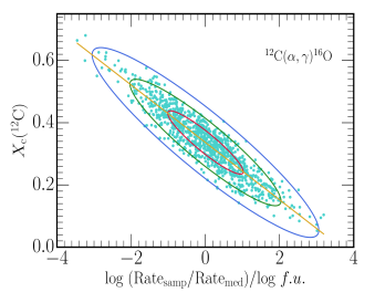
Helium burning is initiated by the triple-$\alpha$ reaction. As isotopes of ¹²C are formed, the proportion of carbon to oxygen is determined by the competition between the carbon-producing triple-$\alpha$ reaction and the carbon-depleting, oxygen-producing radiative capture reaction. The central X_c(¹²C) and X_c(¹⁶O) are strongly anti-correlated with ¹²C($\alpha$,$\gamma$)¹⁶O reaction. In Figure 17 we show the rate variation factor versus the final ¹²C mass fraction at the 1TP. The linear regression yields $R^{2}$=0.854. The production of ¹²C favors a larger $\rho_{\mathrm{c}}$ while the opposite is true for ¹⁶O.

In most cases, the ${}^{12}\textup{C}(\alpha,\gamma)\rm{{}^{16}O}$ reaction dominates the CO core properties. It is only challenged by the triple-$\alpha$ reaction in a vicious battle to consume the remaining He fuel in the final stages of He burning. The relative strength of these channels directly affects the amount ⁴He processed either to ¹²C or ¹⁶O. Recent studies have investigated the affect of altering ${}^{12}\textup{C}(\alpha,\gamma)\rm{{}^{16}O}$ in massive stars using multiplicative rate enhancement factors (West et al., 2013; Tur et al., 2007). Because of the overwhelming impact of this reaction rate, the effect of other H and He burning rates may be overlooked in the assessment of uncertainties in low mass stars. To address this possibility, we consider a grid of Monte Carlo stellar models with a fixed rate distribution for ${}^{12}\textup{C}(\alpha,\gamma)\rm{{}^{16}O}$.

6. With ¹²C($\alpha,\gamma$)¹⁶O Fixed

We evolve an additional grid of 1,000 3 M_⊙ stellar models from the pre-MS to the 1TP, using the same input physics as the grid in §5. Each model uses a fixed rate distribution for ${}^{12}\textup{C}(\alpha,\gamma)\rm{{}^{16}O}$ reaction, the STARLIB median rate distribution, while sampling the 25 remaining reaction rates listed in Table 1.

Figure 18.— Histogram of the 1,000 3 M_⊙ Monte Carlo stellar model grid sampling 25 STARLIB reaction rates. Global and core properties shown include the mass of the CO core (A), age (B), central temperature (C), central density (D), central electron fraction (E), central ²²Ne mass fraction (F), central ¹²C mass fraction (G), and central ¹⁶O mass fraction (H), all at the 1TP. The green dashed lines and the dot dashed red lines denote the 68% and 95% confidence intervals, respectively. The red dashed line denotes the mean value obtained from Table 2 for comparison. The x-axis ranges are the same as in Figure 9.

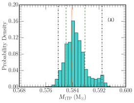
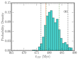
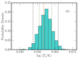
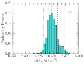
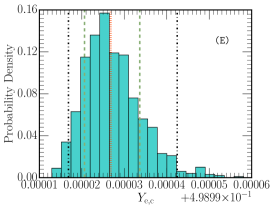
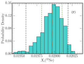
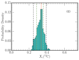
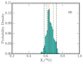
Figure 18 shows histograms of the the mass of the CO core (A), age (B), $T_{\mathrm{\!c}}$ (C), $\rho_{\mathrm{c}}$ (D), $Y_{\rm e,c}$ (E), X_c(²²Ne) (F), X_c(¹²C) (G), and X_c(¹⁶O) (H) at the 1TP. The green dashed lines and the dot-dashed black lines denote the same intervals as in Figure 9. Relative to the arithmetic mean value, we find the width of the 95% confidence interval to be $\Delta M_{{\rm 1TP}}$ $\approx$ 0.013 M_⊙ for the core mass, $\Delta t_{{\rm 1TP}}\approx$ 10.69 Myr for the age, $\Delta\log(T_{{\rm c}}/K)\approx$ 0.011 for the central temperature, $\Delta\log(\rho_{{\rm c}}/{\rm gcm}{-3})\approx$ 0.038 for the central density, $\Delta$$Y_{\rm{e,c}}$ $\approx$ 2.6$\times$10^-5 for the central electron fraction, $\Delta$$X_{\rm{c}}(^{22}\rm{Ne})$ $\approx$ 6.0$\times$10^-4 $\Delta$$X_{\rm{c}}(^{12}\rm{C})$ $\approx$ 0.145, and $\Delta$$X_{\rm{c}}(^{16}\rm{O})$ $\approx$ 0.145. Table 4 lists the arithmetic mean values of the eight quantities shown in Figure 18, the width of the 68% and 95% confidence intervals, and the percentage change from the arithmetic mean using the 95% confidence interval. We use the same methods as in §5 to compare the differences.

!htb Variable Mean 68% C.I. 95% C.I. % Change $M_{\rm{1TP}}$ (M_⊙) 5.850(-1) 5.672(-3) 1.315(-2) 2.248 $t_{\rm{1TP}}$ (Myr) 4.814(2) 5.110 1.069(1) 2.221 log $T_{\rm{c}}$ (K) 8.060 5.723(-3) 1.150(-2) 0.143 log $\rho_{\rm{c}}$ (g cm^-3) 6.351 1.754(-2) 3.790(-2) 0.597 $Y_{\rm{e,c}}$ 4.990(-1) 1.301(-5) 2.562(-5) 0.005 X${}_{\rm{c}}(^{22}$Ne) 1.996(-2) 2.891(-4) 5.961(-4) 2.986 X${}_{\rm{c}}(^{12}$C) 3.235(-1) 7.597(-2) 1.451(-1) 44.85 X${}_{\rm{c}}(^{16}$O) 6.501(-1) 7.610(-2) 1.452(-1) 22.34

Table 4Variations in core quantities - Fixed ¹²C($\alpha,\gamma$)

We compute the eigenvalues and eigenvectors of the correlation matrix as in §5.1. Here we consider 33 quantities in total $-$ the 25 STARLIB reaction rate variation factors in the order listed in Table 1, $M_{{\rm 1TP}}$, $t_{\rm 1TP}$, $T_{\rm{c}}$, $\rho_{\mathrm{c}}$, $Y_{\rm e,c}$, X_c(¹²C), X_c(¹⁶O), and X_c(²²Ne) at the 1TP.

b Component Eigenvalue Proportion Cumulative 1 4.782 0.1449 0.1449 2 3.045 0.0923 0.2372 3 1.802 0.0546 0.2918 4 1.408 0.0427 0.3345 5 1.246 0.0378 0.3722

Table 5Principal Component Analysis - Fixed ¹²C($\alpha,\gamma$)

In Table 5 we show the eigenvalues, proportion of total variation, and cumulative proportion of total variation for the first five principal components. The first five components account for $\approx$ 37% of the total variation with only $\approx$ 14% accounted for by the first component. The amount of variation attributed to the first component is less than that accounted for when the ¹²C($\alpha,\gamma$)¹⁶O is included in the sampling scheme (see Table 3). With a fixed rate distribution, we find less variation. The magnitude of the decrease explained by the first principal component for this grid compared to that found in Table 3 further suggests that the ¹²C($\alpha,\gamma$)¹⁶O dominates the WD composition and structural properties properties. In the limit that all 33 physical quantities are perfectly uncorrelated, the amount of variation accounted for by the first principal component would approach zero. The contrary is true for a system of 33 quantities in which variation among all the quantities can be accounted for by one variable in the set.

The largest positive coefficients in the first principal component are the ¹⁸O($\alpha,\gamma$)²²Ne rate variation factor with a value of +0.473, ¹⁸O($p,\alpha$)¹⁵N with +0.330, and X_c(¹⁶O) with +0.308. The largest negative coefficients are -0.335 for ¹⁸F($p,\alpha$)¹⁵O and -0.326 for ¹⁵O($\alpha,\gamma$)¹⁹Ne. For the second principal component, the largest positive coefficients are +0.413 for X_c(¹²C), +0.412 for X_c(¹⁶O) and +0.371 for ¹⁸F($p,\alpha$)¹⁵O. The largest negative coefficients are -0.214 for $\rho_{\mathrm{c}}$ and -0.156 for ¹⁶O($p,\gamma$)¹⁷F.

We also consider a subset of the data and use a PCA to visualize the differences between the two grids. For example, we consider X_c(¹²C) and the rate variation factor for the triple-$\alpha$ reaction. Using the same steps as in §5.1 we construct a feature vector, w, with the obtained eigenvectors as the columns. Next, we create a new matrix, x, containing our standardized data, where a vector $a$ is transformed to a standardized vector $a^{\prime}$, where $\textbf{a\textprime}=[\textbf{a}-\bar{a}]/\sigma_{a}$, where $\bar{a}$ is the arithmetic mean and $\sigma_{a}$ is the standard deviation of the vector a. We then compute the transformed data using

$$\textbf{y}=\textbf{w}^{\rm{T}}\times\textbf{x}~{}.$$ (9)

Figure 19.— Transformed data for X_c(¹²C) versus the rate variation factor for triple-$\alpha$ for the grid of 1,000 3 M_⊙ Monte Carlo stellar models sampling 26 STARLIB reaction rates shown along the first and second principal components. The dashed lines denote the eigenvectors of the correlation matrix.

Figure 20.— Same as in Figure 19 but for the grid of Monte Carlo stellar models sampling 25 STARLIB reaction rates and fixed rate distribution for ¹²C($\alpha,\gamma$)¹⁶O.

Figure 21.— Spearman rank correlation coefficients for the 25 independently sampled nuclear reaction rates for 1,000 Monte Carlo stellar models with a ZAMS mass of 3 M_⊙. The rate identifiers correspond to those listed in Table 1. Each sampled rate is compared individually against the final mass of the CO core ($M_{{\rm 1TP}}$, A), age of stellar model ($t_{{\rm 1TP}}$, B), central temperature ($T_{{\rm c}}$, C), central density ($\rho_{{\rm c}}$, D), central electron fraction ($T_{{\rm e,c}}$, E), central ²²Ne mass fraction (X_c(²²Ne), F), central ¹²C mass fraction (X_c(¹²C), G), and central ¹⁶O mass fraction (X_c(¹⁶O), H) at the 1TP.

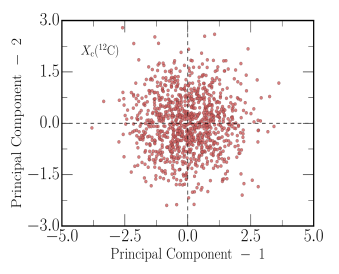
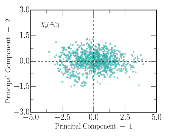
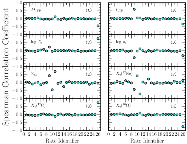
Figure 19 shows the linear transformation for the rate variation factor for the triple-$\alpha$ reaction and X_c(¹²C) for the grid of stellar models that sampled 26 STARLIB rates (including the ¹²C($\alpha,\gamma$)¹⁶O reaction). We find considerable variation along the first and second principal component. The proportion of variation explained by the first component shown is $\approx$ 63%.

Figure 20 shows the linear transformation for the triple-$\alpha$ rate variation factor and X_c(¹²C) for the grid of stellar models that sampled 25 STARLIB rates while using the median STARLIB rate distribution for ¹²C($\alpha,\gamma$)¹⁶O. In contrast to Figure 19, the first principal component holds the majority of the variation, $\approx$ 88%. This result suggests that when the ¹²C($\alpha,\gamma$)¹⁶O reaction is considered in the sampling scheme, it can overpower triple-$\alpha$. Specifically, the first principal component accounts for only a $\approx$ 63% proportion of variation between the triple-$\alpha$ reaction and X_c(¹²C) - see Figure 20.

Figure 22.— IFMR of 153 stellar models evolved from the pre-MS to the final WD stage. Initial masses ranged between 1-6 M_⊙ in steps of 0.1 M_⊙ utilizing the low, median, and high reaction rate distributions for the 26 STARLIB sampled rates given in Table 1. Filled circles show the median final mass value, while the error bars denote the low and upper limits found from the remaining two models. Progenitor masses from the observations were inferred from PARSEC isochrones. See Bressan et al. (2012) and Dotter (2016) for details.

Figure 23.— IFMR residuals for 4.0 M_⊙ $\lesssim$ $M_{i}\lesssim$ 6.6 M_⊙. The legend is the same as in Figure 22.

In Figure 21, we show the Spearman coefficients against the 25 independently sampled rate variation factors for $M_{{\rm 1TP}}$, $t_{{\rm 1TP}}$, $T_{{\rm c}}$, $\rho_{{\rm c}}$, $Y_{\rm e,c}$, X_c(²²Ne), X_c(¹²C), and X_c(¹⁶O), at the 1TP. In the previous section, $M_{{\rm 1TP}}$ was dominated by the uncertainties in the ${}^{12}\textup{C}(\alpha,\gamma)\rm{{}^{16}O}$ and triple-$\alpha$ reaction. Here, the mass of the CO core at the 1TP is still affected by the triple-$\alpha$ reaction with a Spearman coefficient of $r_{\mathrm{s}}$=-0.45. However, we also find that the ${}^{15}\textup{N}(p,\gamma)\rm{{}^{16}O}$, has a larger effect in the absence of the ${}^{12}\textup{C}(\alpha,\gamma)\rm{{}^{16}O}$ reaction, with a coefficient of $r_{\mathrm{s}}$=+0.12.

For $t_{{\rm 1TP}}$, it is still dominated by the uncertainties in ${}^{14}\textup{N}(p,\gamma)\rm{{}^{15}O}$ and triple-$\alpha$, but for a fixed ${}^{12}\textup{C}(\alpha,\gamma)\rm{{}^{16}O}$ distribution we find increases in Spearman coefficients $r_{\mathrm{s}}$=(+0.60,-0.33), an increase of $\approx$ 22% and $\approx$ 43%, respectively.

$T_{{\rm c}}$ is again most affected by ${}^{14}\textup{N}(p,\gamma)\rm{{}^{15}O}$ and triple-$\alpha$ with $r_{\mathrm{s}}$=(0.18,+0.76) respectively. Previously unidentified, $\rho_{{\rm c}}$ is correlated with ${}^{14}\textup{N}(p,\gamma)\rm{{}^{15}O}$ with $r_{\mathrm{s}}$=-0.43. Additionally, we see a dependence triple-$\alpha$ with $r_{\mathrm{s}}$=-0.31. $Y_{{\rm e,c}}$, was dominated by individual reactions of the CNO cycle in the previous section. Here we find similar results with $r_{\mathrm{s}}$= (+0.44,-0.44,+0.70) corresponding to ${}^{14}\textup{N}(p,\gamma)\rm{{}^{15}O}$, ${}^{15}\textup{N}(p,\alpha)\rm{{}^{12}C}$, and ${}^{15}\textup{N}(p,\gamma)\rm{{}^{16}O}$, respectively. X_c(²²Ne) is again anti-correlated with $Y_{{\rm e,c}}$ with similar coefficients of $r_{\mathrm{s}}$=(-0.42,+0.43,-0.70), corresponding to the same CNO reactions.

The central X_c(¹²C) and X_c(¹⁶O) show the largest change for a fixed ${}^{12}\textup{C}(\alpha,\gamma)\rm{{}^{16}O}$. Previously, we found large Spearman coefficients between the ${}^{12}\textup{C}(\alpha,\gamma)\rm{{}^{16}O}$ reaction and X_c(¹²C) and X_c(¹⁶O) with $r_{\mathrm{s}}$=(-0.91, +0.91), respectively. This suggested X_c(¹²C) and X_c(¹⁶O) could be mostly determined by one reaction. However, for a fixed ${}^{12}\textup{C}(\alpha,\gamma)\rm{{}^{16}O}$ rate distribution, the triple-$\alpha$ reaction dominates the variation. For X_c(¹²C) and X_c(¹⁶O) and triple-$\alpha$ we find $r_{\mathrm{s}}$= (+0.75,-0.75), respectively. This represents an approximately 300% increase in magnitude of the Spearman coefficients found in the first grid sampling the 26 STARLIB rates. Moreover, a value of $r_{\mathrm{s}}$=0.1 is found for the rate variation factor for ${}^{15}\textup{N}(p,\gamma)\rm{{}^{16}O}$ and X_c(¹²C) and $r_{\mathrm{s}}$=-0.1 for ${}^{15}\textup{N}(p,\gamma)\rm{{}^{16}O}$ and X_c(¹⁶O). This suggests that when neglecting the dominant effect of the main radiative alpha capture reaction, ${}^{12}\textup{C}(\alpha,\gamma)\rm{{}^{16}O}$, the proton capture rate, ${}^{15}\textup{N}(p,\gamma)\rm{{}^{16}O}$ can have an effect on the final ¹²C and ¹⁶O abundances.

7. Initial-Final Mass Relationship

The question then naturally arises: what is the impact of the uncertainties in the nuclear reaction rates on the IFMR? To address this question, we evolved a third grid of MESA models from the pre-MS through the thermally pulsing AGB phase to the final formation of the CO WD. Our grid consists of 153 models from 1-6 M_⊙ in steps of 0.1 M_⊙ using the STARLIB low, med, and high rate distributions for the 26 sampled rates, for a total of 3 models at each mass point. Our goal is to quantify the effect of composite uncertainties in thermonuclear reaction rates on the properties of the final CO WD. The models are evolved from the pre-MS until the mass of the H-rich envelope has reached a minimum value of $M_{\rm{env}}=0.01$ M_⊙. The grid uses the same input physics as in §2, with the exception that we increase the efficiency of mass loss on the RBG and AGB to $\eta$=0.7. This increase in mass loss efficiency allows our grid to evolve to the our specified MESA stopping condition in a computationally efficient manner. Moreover, increased efficiency in the mass loss has been shown to alter characteristics of the TP phase, but yield only modest affects on the final WD (Andrews et al., 2015). Each model required $\approx$ 96 hours on 12 cores for each of the 153 models to go from the pre-MS to the final WD, a total of $\approx$ 176,000 core-hours.

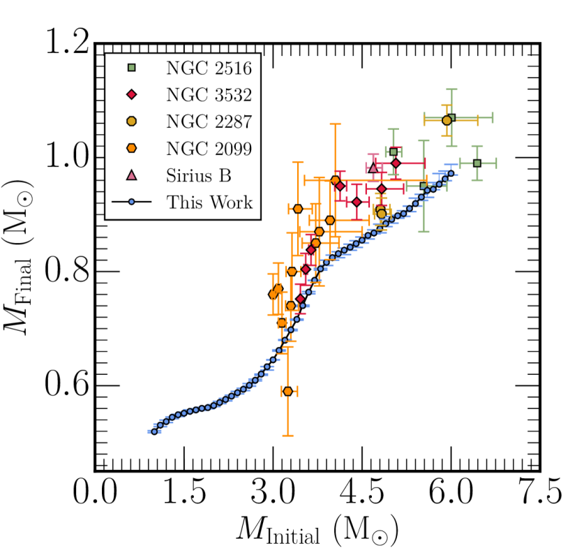
In Figure 22 we show the IFMR resulting from our grid of stellar models. The filled circles shown in Figure 22, are the median STARLIB values, while the lower and upper STARLIB limits are denoted by the blue error bars. We compare our models to observational data for the solar metallicity cluster NGC 2516 (Catalán et al., 2008), NGC 2099 (Cummings et al., 2015), NGC 3532, NGC 2287, and Sirius B (assuming solar metallicity) from Cummings et al. (2016). The observational data focuses on WD candidates with inferred solar metallicity. However, the IFMR has been shown to depend significantly on the initial progenitor metallicity, shifting the trend towards higher final WD masses (Meng et al., 2008; Romero et al., 2015). The observational data for inferred initial progenitor WD masses below 3 M_⊙ have been excluded from this comparison as the majority these WDs are from supersolar metallicity clusters such as NGC 6791 or the host environments remain largely uncertain (Kalirai et al., 2008; Zhao et al., 2012, and references therein).

In most cases, the most massive WD model for a chosen initial mass has the low reaction rate distributions. For decreased nuclear burning efficiency, the He burning shell has a prolonged lifetime allowing for a more massive CO core to grow. For all three models at each mass point, the final CO masses agree within $\approx$ $\pm$ 0.003 M_⊙.

A noticeable feature of Figure 22 is that the mean trend of our models tend to lie below the observational trend. This discrepancy is likely due to our choices for the mixing parameters. The largest assumption is probably the efficiency of convective overshoot being uniform at all boundary layers. To address this discrepancy, we evolved an additional 3 M_⊙ model without convective overshoot, $f_{\rm{ov}}=0.00$ at all boundaries, using the med STARLIB rates. Our 3 M_⊙ model with $f_{\rm{ov}}=0.016$ resulted in a final CO WD mass of $\approx$ 0.645 M_⊙. However, we found that the model without convective overshoot yielded a final CO WD mass of $\approx$ 0.684 M_⊙. This suggests that the discrepancy between the mean trend of our IFMR and the observational data is a result of our of choices for efficiency of convective overshoot.

Following Andrews et al. (2015), we fit our IFMR in three distinct regimes: $M_{i}\lesssim$ 2.5 M_⊙ experience a degenerate He shell flash (Sweigart & Gross, 1978; Suda et al., 2011), 2.5 $M_{i}\lesssim$ 4 M_⊙, undergo stable He core burning, while for $M_{i}\geq$ 4 M_⊙ the second dredge-up becomes important (Dominguez et al., 1999; Herwig, 2000). We construct a piece-wise linear function to the IFMR with turnover points at 2.5 M_⊙ and 4 M_⊙:

$$\begin{split}M_{\rm{f}}/M_{\odot}=&(0.0422\pm 0.002)M_{\rm{i}}+(0.4851\pm 0.004)\\ &\qquad{\rm for}\ M_{\rm{i}}\lesssim 2.5M_{\odot}\\ =&(0.1686\pm 0.006)M_{\rm{i}}+(0.1516\pm 0.019)\\ &\qquad{\rm for}\ 2.5\lesssim M_{\rm{i}}\lesssim 4.0M_{\odot}\\ =&(0.0734\pm 0.001)M_{\rm{i}}+(0.5265\pm 0.006)\\ &\qquad{\rm for}\ 4.0\lesssim M_{\rm{i}}\lesssim 7.0M_{\odot}\end{split}$$ (10)

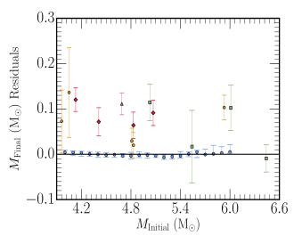
Our 7.0 M_⊙ upper limit is based on estimates of the lowest mass for carbon ignition (Farmer et al., 2015, and references therein). Figure 23 shows the final mass residuals using Equation (10). The upper and lower WD masses derived from the MESA models agree to $\approx$ $\pm 0.008$ M_⊙, while the observations agree to within $\approx$ $\pm 0.12$ M_⊙.

8. Summary and Conclusions

We have investigated the properties of CO cores evolved from the pre-MS using the first complete Monte Carlo stellar models. We evolved two grids of stellar models: (1) 1,000 3 M_⊙ Monte Carlo stellar models sampling 26 STARLIB nuclear reaction rates from pre-MS to the 1TP, (2) 1,000 3 M_⊙ Monte Carlo stellar models using the median STARLIB rate distribution for ¹²C($\alpha,\gamma$)¹⁶O while sampling the remaining 25 STARLIB rates from pre-MS to the 1TP. We used a Principal Component Analysis and Spearman Rank-Order Correlation to quantify the variation of the mass of the CO core, age, central temperature, central density, central electron fraction, central ²²Ne mass fraction, central ¹²C mass fraction, and central ¹⁶O mass fraction, all at the 1TP.

When sampling 26 STARLIB reaction rates (including the ¹²C($\alpha,\gamma$)¹⁶O reaction), we found that the experimental uncertainties in the ¹²C($\alpha,\gamma)^{16}\rm{O}$, triple-$\alpha$, and ¹⁴N($p,\gamma)^{15}\rm{O}$ reactions dominated the properties of the stellar model. The largest changes were found for the ¹²C and ¹⁶O mass fractions. In particular, we found a percent change of $\approx$ 116% and $\approx$ 62% from the arithmetic mean value using the 95% confidence interval for the ¹²C and ¹⁶O mass fractions, respectively. The remaining six quantities had percent changes $\lesssim$ 4%. This result suggests that the relative abundances ¹²C and ¹⁶O can can vary significantly within experimental uncertainties, while other quantities are well constrained.

Using a fixed rate distribution for the ¹²C($\alpha,\gamma$)¹⁶O reaction and sampling the remaining 25 STARLIB rates, we found that the triple-$\alpha$ and ¹⁴N($p,\gamma)^{15}\rm{O}$ reactions still play a significant role. However, additional rates such as the ${}^{15}\textup{N}(p,\gamma)\rm{{}^{16}O}$ reaction were found to have non-negligible effects on the final core mass, $X_{\rm{c}}(^{12}$C) and $X_{\rm{c}}$$(^{16}$O). Moreover, we $\approx$ 45% and $\approx$ 22% changes from the arithmetic mean value using the 95% confidence interval for the ¹²C and ¹⁶O mass fractions, respectively. The remaining six quantities had percent changes $\lesssim$ 3%. This suggests that the results of our Monte Carlo stellar evolution studies is dependent on the reaction rates considered in the sampling scheme. Additionally, our results suggest that the experimental uncertainties in the ¹²C($\alpha,\gamma$)¹⁶O reaction has a larger impact than triple-$\alpha$ on the final CO WD chemical composition.

To quantify the role of uncertainties in the nuclear reaction rates on the the IFMR, we evolved a third grid of MESA models from the pre-MS through the thermally pulsing AGB phase to the final formation of the CO WD. Our grid consisted of 153 models from 1-6 M_⊙ in steps of 0.1 M_⊙ using the STARLIB low, med, and high rate distributions for the 26 sampled rates, for a total of 3 models at each mass point. We showed that the final WD masses using each set of reactions agreed to within $\approx$ $\pm$ 0.003 M_⊙. This result suggests that uncertainties in the final mass relative to the nuclear reaction rates are well constrained.

The mean trend of our IFMR stellar models was found to lie below that of the observational trend. Differences were found to be attributed to the efficiency of different mixing processes in our models. Salaris et al. (2009) found that the inclusion of convective overshoot on the MS is needed to for agreement with observational constraints. However, too efficient convective overshoot during the AGB phase can also inhibit the growth of the CO core during the TP-AGB phase. 3D hydrodynamic simulations of He-shell flash convection suggests a more modest core overshoot value during the AGB phase (Herwig et al., 2006). We found that evolving a 3 M_⊙ model with the median STARLIB rates, but without convective overshoot yielded a final CO WD mass of $\approx$ 0.684 M_⊙ while our model with $f_{\rm{ov}}=0.016$ had a final mass of $\approx$ 0.645 M_⊙. Future efforts could include other parameters in the Monte Carlo sampling scheme, such as the efficiency of convective overshoot at different boundaries, to identify the largest areas of uncertainty in the evolution and formation of CO WDs.

References

- Agertz & Kravtsov (2015) Agertz, O., & Kravtsov, A. V. 2015, ApJ, 804, 18
- Alastuey & Jancovici (1978) Alastuey, A., & Jancovici, B. 1978, ApJ, 226, 1034
- Althaus et al. (2010) Althaus, L. G., Córsico, A. H., Isern, J., & García-Berro, E. 2010, A&A Rev., 18, 471
- An et al. (2015) An, Z.-D., Chen, Z.-P., Ma, Y.-G., et al. 2015, Phys. Rev. C, 92, 045802
- Andrews et al. (2015) Andrews, J. J., Agüeros, M. A., Gianninas, A., et al. 2015, ApJ, 815, 63
- Angulo et al. (1999) Angulo, C., Arnould, M., Rayet, M., et al. 1999, Nuclear Physics A, 656, 3
- Blöcker (1995) Blöcker, T. 1995, A&A, 297, 727
- Boothroyd & Sackmann (1988) Boothroyd, A. I., & Sackmann, I.-J. 1988, ApJ, 328, 653
- Bressan et al. (2012) Bressan, A., Marigo, P., Girardi, L., et al. 2012, MNRAS, 427, 127
- Buchmann (1996) Buchmann, L. 1996, ApJ, 468, L127
- Buckner et al. (2015) Buckner, M. Q., Iliadis, C., Kelly, K. J., et al. 2015, Phys. Rev. C, 91, 015812
- Catalán et al. (2008) Catalán, S., Isern, J., García-Berro, E., et al. 2008, A&A, 477, 213
- Caughlan & Fowler (1988) Caughlan, G. R., & Fowler, W. A. 1988, Atomic Data and Nuclear Data Tables, 40, 283
- Chernykh et al. (2010) Chernykh, M., Feldmeier, H., Neff, T., von Neumann-Cosel, P., & Richter, A. 2010, Physical Review Letters, 105, 022501
- Childress et al. (2013) Childress, M., Aldering, G., Antilogus, P., et al. 2013, ApJ, 770, 107
- Cummings et al. (2015) Cummings, J. D., Kalirai, J. S., Tremblay, P.-E., & Ramirez-Ruiz, E. 2015, ApJ, 807, 90
- Cummings et al. (2016) —. 2016, ArXiv e-prints, arXiv:1601.03053
- Cyburt & Davids (2008) Cyburt, R. H., & Davids, B. 2008, Phys. Rev. C, 78, 064614
- Cyburt et al. (2010a) Cyburt, R. H., Ellis, J., Fields, B. D., et al. 2010a, ArXiv e-prints, arXiv:1007.4173
- Cyburt et al. (2010b) Cyburt, R. H., Amthor, A. M., Ferguson, R., et al. 2010b, ApJS, 189, 240
- deBoer et al. (2013) deBoer, R. J., Görres, J., Imbriani, G., et al. 2013, Phys. Rev. C, 87, 015802
- Descouvemont et al. (2004) Descouvemont, P., Adahchour, A., Angulo, C., Coc, A., & Vangioni-Flam, E. 2004, Atomic Data and Nuclear Data Tables, 88, 203
- Dobbie et al. (2006) Dobbie, P. D., Napiwotzki, R., Burleigh, M. R., et al. 2006, MNRAS, 369, 383
- Dominguez et al. (1999) Dominguez, I., Chieffi, A., Limongi, M., & Straniero, O. 1999, ApJ, 524, 226
- Dotter (2016) Dotter, A. 2016, ApJS, 222, 8
- Eisenstein et al. (2006) Eisenstein, D. J., Liebert, J., Harris, H. C., et al. 2006, ApJS, 167, 40
- Evans et al. (2000) Evans, M., Hastings, N., & Peacock, B. 2000, Statistical Distributions, 3rd edn. (Hoboken, NJ: Wiley)
- Farmer et al. (2015) Farmer, R., Fields, C. E., & Timmes, F. X. 2015, ApJ, 807, 184
- Fuller et al. (1985) Fuller, G. M., Fowler, W. A., & Newman, M. J. 1985, ApJ, 293, 1
- Goriely et al. (2008) Goriely, S., Hilaire, S., & Koning, A. J. 2008, A&A, 487, 767
- Greggio (2010) Greggio, L. 2010, MNRAS, 406, 22
- Grevesse & Sauval (1998) Grevesse, N., & Sauval, A. J. 1998, Space Sci. Rev., 85, 161
- Hansen & Liebert (2003) Hansen, B. M. S., & Liebert, J. 2003, ARA&A, 41, 465
- Hansen et al. (2004) Hansen, C. J., Kawaler, S. D., & Trimble, V. 2004, Stellar interiors : physical principles, structure, and evolution (New York: Springer-Verlag)
- Herwig (2000) Herwig, F. 2000, A&A, 360, 952
- Herwig et al. (2006) Herwig, F., Freytag, B., Hueckstaedt, R. M., & Timmes, F. X. 2006, ApJ, 642, 1057
- Heyer & Schloerb (1997) Heyer, M. H., & Schloerb, F. P. 1997, The Astrophysical Journal, 475, 173
- Howell et al. (2009) Howell, D. A., Sullivan, M., Brown, E. F., et al. 2009, ApJ, 691, 661
- Hoyle (1954) Hoyle, F. 1954, ApJS, 1, 121
- Iben (1991) Iben, Jr., I. 1991, ApJS, 76, 55
- Iben (2013a) —. 2013a, Stellar Evolution Physics, Volume 1: Physical Processes in Stellar Interiors (Cambridge, UK: Cambridge University Press)
- Iben (2013b) —. 2013b, Stellar Evolution Physics, Volume 2: Advanced Evolution of Single Stars (Cambridge, UK: Cambridge University Press)
- Iliadis (2007) Iliadis, C. 2007, Nuclear Physics of Stars (Wiley-VCH Verlag)
- Iliadis et al. (2002) Iliadis, C., Champagne, A., José, J., Starrfield, S., & Tupper, P. 2002, ApJS, 142, 105
- Iliadis et al. (2001) Iliadis, C., D’Auria, J. M., Starrfield, S., Thompson, W. J., & Wiescher, M. 2001, ApJS, 134, 151
- Iliadis et al. (2010a) Iliadis, C., Longland, R., Champagne, A. E., & Coc, A. 2010a, Nuclear Physics A, 841, 251
- Iliadis et al. (2010b) Iliadis, C., Longland, R., Champagne, A. E., Coc, A., & Fitzgerald, R. 2010b, Nuclear Physics A, 841, 31
- Iliadis et al. (2015) Iliadis, C., Longland, R., Coc, A., Timmes, F. X., & Champagne, A. E. 2015, Journal of Physics G Nuclear Physics, 42, 034007
- Imbriani et al. (2005) Imbriani, G., Costantini, H., Formicola, A., et al. 2005, European Physical Journal A, 25, 455
- Itoh et al. (1996) Itoh, N., Hayashi, H., Nishikawa, A., & Kohyama, Y. 1996, ApJS, 102, 411
- Itoh et al. (1979) Itoh, N., Totsuji, H., Ichimaru, S., & Dewitt, H. E. 1979, ApJ, 234, 1079
- Jackson (2005) Jackson, J. E. 2005, A user’s guide to principal components, Vol. 587 (John Wiley & Sons)
- Jolliffe (2002) Jolliffe, I. T. 2002, Principal Component Analysis, 2nd edn., Springer Series in Statistics (Springer-Verlag New York)
- Kalirai (2012) Kalirai, J. S. 2012, Nature, 486, 90
- Kalirai et al. (2008) Kalirai, J. S., Hansen, B. M. S., Kelson, D. D., et al. 2008, ApJ, 676, 594
- Kalirai et al. (2009) Kalirai, J. S., Zucker, D. B., Guhathakurta, P., et al. 2009, ApJ, 705, 1043
- Karakas & Lattanzio (2007) Karakas, A., & Lattanzio, J. C. 2007, PASA, 24, 103
- Kepler et al. (2007) Kepler, S. O., Kleinman, S. J., Nitta, A., et al. 2007, MNRAS, 375, 1315
- Kepler et al. (2015) Kepler, S. O., Pelisoli, I., Koester, D., et al. 2015, MNRAS, 446, 4078
- Kepler et al. (2016) —. 2016, MNRAS, 455, 3413
- Kilic et al. (2009) Kilic, M., Gould, A., & Koester, D. 2009, ApJ, 705, 1219
- Kistler et al. (2013) Kistler, M. D., Stanek, K. Z., Kochanek, C. S., Prieto, J. L., & Thompson, T. A. 2013, ApJ, 770, 88
- Koester (2002) Koester, D. 2002, A&A Rev., 11, 33
- Kunz et al. (2002) Kunz, R., Fey, M., Jaeger, M., et al. 2002, ApJ, 567, 643
- Lane (2013) Lane, D. 2013, Online Statistics Education: A Multimedia Course of Study (Rice University)
- Langanke & Martínez-Pinedo (2000) Langanke, K., & Martínez-Pinedo, G. 2000, Nuclear Physics A, 673, 481
- Lattanzio (1991) Lattanzio, J. C. 1991, ApJS, 76, 215
- Leitner & Kravtsov (2011) Leitner, S. N., & Kravtsov, A. V. 2011, ApJ, 734, 48
- Longland (2012) Longland, R. 2012, A&A, 548, A30
- Longland et al. (2010) Longland, R., Iliadis, C., Champagne, A. E., et al. 2010, Nuclear Physics A, 841, 1
- LUNA Collaboration et al. (2006) LUNA Collaboration, Lemut, A., Bemmerer, D., et al. 2006, Physics Letters B, 634, 483
- Magkotsios et al. (2010) Magkotsios, G., Timmes, F. X., Hungerford, A. L., et al. 2010, ApJS, 191, 66
- Marigo et al. (1996) Marigo, P., Bressan, A., & Chiosi, C. 1996, A&A, 313, 545
- Marigo et al. (1998) —. 1998, A&A, 331, 564
- Meng et al. (2008) Meng, X., Chen, X., & Han, Z. 2008, A&A, 487, 625
- Metcalfe et al. (2002) Metcalfe, T. S., Salaris, M., & Winget, D. E. 2002, ApJ, 573, 803
- Moreno-Raya et al. (2015) Moreno-Raya, M. E., Mollá, M., López-Sánchez, Á. R., et al. 2015, ArXiv e-prints, arXiv:1511.05348
- Neill et al. (2009) Neill, J. D., Sullivan, M., Howell, D. A., et al. 2009, ApJ, 707, 1449
- Oda et al. (1994) Oda, T., Hino, M., Muto, K., Takahara, M., & Sato, K. 1994, Atomic Data and Nuclear Data Tables, 56, 231
- Parikh et al. (2008) Parikh, A., José, J., Moreno, F., & Iliadis, C. 2008, ApJS, 178, 110
- Parikh et al. (2013) Parikh, A., José, J., Seitenzahl, I. R., & Röpke, F. K. 2013, A&A, 557, A3
- Paxton et al. (2011) Paxton, B., Bildsten, L., Dotter, A., et al. 2011, ApJS, 192, 3
- Paxton et al. (2013) Paxton, B., Cantiello, M., Arras, P., et al. 2013, ApJS, 208, 4
- Paxton et al. (2015) Paxton, B., Marchant, P., Schwab, J., et al. 2015, ApJS, 220, 15
- Pritchet et al. (2008) Pritchet, C. J., Howell, D. A., & Sullivan, M. 2008, ApJ, 683, L25
- Raddi et al. (2016) Raddi, R., Catalan, S., Gaensicke, B. T., et al. 2016, ArXiv e-prints, arXiv:1601.02019
- Rauscher & Thielemann (2000) Rauscher, T., & Thielemann, F.-K. 2000, Atomic Data and Nuclear Data Tables, 75, 1
- Reimers (1975) Reimers, D. 1975, Memoires of the Societe Royale des Sciences de Liege, 8, 369
- Roberts et al. (2006) Roberts, L. F., Hix, W. R., Smith, M. M., & Fisker, J. L. 2006, in Proc. Science, 1–6
- Romero et al. (2015) Romero, A. D., Campos, F., & Kepler, S. O. 2015, MNRAS, 450, 3708
- Romero et al. (2012) Romero, A. D., Córsico, A. H., Althaus, L. G., et al. 2012, MNRAS, 420, 1462
- Romero et al. (2013) Romero, A. D., Kepler, S. O., Córsico, A. H., Althaus, L. G., & Fraga, L. 2013, ApJ, 779, 58
- Safarzadeh et al. (2016) Safarzadeh, M., Hayward, C. C., Ferguson, H. C., & Somerville, R. S. 2016, ApJ, 818, 62
- Salaris et al. (1997) Salaris, M., Domínguez, I., García-Berro, E., et al. 1997, ApJ, 486, 413
- Salaris et al. (2009) Salaris, M., Serenelli, A., Weiss, A., & Miller Bertolami, M. 2009, ApJ, 692, 1013
- Sallaska et al. (2013) Sallaska, A. L., Iliadis, C., Champange, A. E., et al. 2013, ApJS, 207, 18
- Shingles et al. (2015) Shingles, L. J., Doherty, C. L., Karakas, A. I., et al. 2015, MNRAS, 452, 2804
- Singh et al. (1998) Singh, H. P., Gulati, R. K., & Gupta, R. 1998, MNRAS, 295, 312
- Stoesz & Herwig (2003) Stoesz, J. A., & Herwig, F. 2003, MNRAS, 340, 763
- Straniero et al. (2003) Straniero, O., Domínguez, I., Imbriani, G., & Piersanti, L. 2003, ApJ, 583, 878
- Suda et al. (2011) Suda, T., Hirschi, R., & Fujimoto, M. Y. 2011, ApJ, 741, 61
- Sweigart & Gross (1978) Sweigart, A. V., & Gross, P. G. 1978, ApJS, 36, 405
- Townsley et al. (2009) Townsley, D. M., Jackson, A. P., Calder, A. C., et al. 2009, ApJ, 701, 1582
- Tur et al. (2007) Tur, C., Heger, A., & Austin, S. M. 2007, ApJ, 671, 821
- Walt et al. (2011) Walt, S. v. d., Colbert, S. C., & Varoquaux, G. 2011, Computing in Science & Engineering, 13, 22
- Weaver & Woosley (1993) Weaver, T. A., & Woosley, S. E. 1993, Phys. Rep., 227, 65
- Weidemann (2000) Weidemann, V. 2000, A&A, 363, 647
- West et al. (2013) West, C., Heger, A., & Austin, S. M. 2013, ApJ, 769, 2
- Williams et al. (2009) Williams, K. A., Bolte, M., & Koester, D. 2009, ApJ, 693, 355
- Zhao et al. (2012) Zhao, J. K., Oswalt, T. D., Willson, L. A., Wang, Q., & Zhao, G. 2012, ApJ, 746, 144