Admissible state and physical constraints preserving schemes for relativistic magnetohydrodynamic equations

Kailiang Wu School of Mathematical Sciences
Peking University
Beijing 100871, P.R. China
wukl@pku.edu.cn
 and  Huazhong Tang HEDPS, CAPT & LMAM, School of Mathematical Sciences
Peking University
Beijing 100871, P.R. China
hztang@math.pku.edu.cn
Abstract.

This paper first studies the admissible state set 𝒢𝒢\mathcal{G} of relativistic magnetohydrodynamics (RMHD). It paves a way for developing physical-constraints-preserving (PCP) schemes for the RMHD equations with the solutions in 𝒢𝒢\mathcal{G}. To overcome the difficulties arising from the extremely strong nonlinearities and no explicit formulas of the primitive variables and the flux vectors with respect to the conservative vector, two equivalent forms of 𝒢𝒢\mathcal{G} with explicit constraints on the conservative vector are skillfully discovered. The first is derived by analyzing roots of several polynomials and transferring successively them, and further used to prove the convexity of 𝒢𝒢\mathcal{G} with the aid of semi-positive definiteness of the second fundamental form of a hypersurface. While the second is derived based on the convexity, and then used to show the orthogonal invariance of 𝒢𝒢\mathcal{G}. The Lax-Friedrichs (LxF) splitting property does not hold generally for the nonzero magnetic field, but by a constructive inequality and pivotal techniques, we discover the generalized LxF splitting properties, combining the convex combination of some LxF splitting terms with a discrete divergence-free condition of the magnetic field.

Based on the above analyses, several one- and two-dimensional PCP schemes are then studied. In the 1D case, a first-order accurate LxF type scheme is first proved to be PCP under the Courant-Friedrichs-Lewy (CFL) condition, and then the high-order accurate PCP schemes are proposed via a PCP limiter. In the 2D case, the discrete divergence-free condition and PCP property are analyzed for a first-order accurate LxF type scheme, and two sufficient conditions are derived for high-order accurate PCP schemes. Our analysis reveals in theory for the first time that the discrete divergence-free condition is closely connected with the PCP property. Several numerical examples demonstrate the theoretical findings and the performance of numerical schemes.

1. Introduction

The paper is concerned with establishing mathematical properties on the admissible state set and developing physical-constraints-preserving (PCP) numerical schemes (which preserve the positivity of the density and pressure, and the bound of the fluid velocity) for special relativistic magnetohydrodynamics (RMHD). The d𝑑d-dimensional governing equations of the special RMHDs is a first-order quasilinear hyperbolic system, see e.g. [18], and in the laboratory frame, it can be written in the divergence form

𝑼t+i=1d𝑭i(𝑼)xi=𝟎,𝑼𝑡superscriptsubscript𝑖1𝑑subscript𝑭𝑖𝑼subscript𝑥𝑖0\frac{{\partial\mbox{\boldmath\small$U$}}}{{\partial t}}+\sum\limits_{i=1}^{d}{\frac{{\partial{\mbox{\boldmath\small$F$}_{i}}(\mbox{\boldmath\small$U$})}}{{\partial x_{i}}}}=\mbox{\boldmath\small$0$}, (1.1)

together with the divergence-free condition on the magnetic field 𝑩=(B1,B2,B3)𝑩subscript𝐵1subscript𝐵2subscript𝐵3\mbox{\boldmath\small$B$}=(B_{1},B_{2},B_{3}), i.e.

i=1dBixi=0,superscriptsubscript𝑖1𝑑subscript𝐵𝑖subscript𝑥𝑖0\sum\limits_{i=1}^{d}\frac{\partial B_{i}}{\partial x_{i}}=0, (1.2)

where d=1𝑑1d=1, or 2 or 3, and 𝑼𝑼U and 𝑭i(𝑼)subscript𝑭𝑖𝑼\mbox{\boldmath\small$F$}_{i}(\mbox{\boldmath\small$U$}) denote the conservative vector and the flux in the xisubscript𝑥𝑖x_{i}-direction, respectively, defined by

𝑼=(D,𝒎,𝑩,E),𝑼superscript𝐷𝒎𝑩𝐸top\displaystyle\mbox{\boldmath\small$U$}=\big{(}D,\mbox{\boldmath\small$m$},\mbox{\boldmath\small$B$},E\big{)}^{\top},
𝑭i(𝑼)=(Dvi,vi𝒎Bi(W2𝑩+(𝒗𝑩)𝒗)+ptot𝒆i,vi𝑩Bi𝒗,mi),i=1,,d,formulae-sequencesubscript𝑭𝑖𝑼superscript𝐷subscript𝑣𝑖subscript𝑣𝑖𝒎subscript𝐵𝑖superscript𝑊2𝑩𝒗𝑩𝒗subscript𝑝𝑡𝑜𝑡subscript𝒆𝑖subscript𝑣𝑖𝑩subscript𝐵𝑖𝒗subscript𝑚𝑖top𝑖1𝑑\displaystyle\mbox{\boldmath\small$F$}_{i}(\mbox{\boldmath\small$U$})=\bigg{(}Dv_{i},v_{i}\mbox{\boldmath\small$m$}-B_{i}\Big{(}W^{-2}\mbox{\boldmath\small$B$}+(\mbox{\boldmath\small$v$}\cdot\mbox{\boldmath\small$B$})\mbox{\boldmath\small$v$}\Big{)}+p_{tot}\mbox{\boldmath\small$e$}_{i},v_{i}\mbox{\boldmath\small$B$}-B_{i}\mbox{\boldmath\small$v$},m_{i}\bigg{)}^{\top},\quad i=1,\cdots,d,

with the mass density D=ρW𝐷𝜌𝑊D=\rho W, the momentum density (row) vector 𝒎=ρhW2𝒗+|𝑩|2𝒗(𝒗𝑩)𝑩𝒎𝜌superscript𝑊2𝒗superscript𝑩2𝒗𝒗𝑩𝑩\mbox{\boldmath\small$m$}=\rho h{W^{2}}\mbox{\boldmath\small$v$}+|\mbox{\boldmath\small$B$}{|^{2}}\mbox{\boldmath\small$v$}-(\mbox{\boldmath\small$v$}\cdot\mbox{\boldmath\small$B$})\mbox{\boldmath\small$B$}, the energy density E=ρhW2ptot+|𝑩|2𝐸𝜌superscript𝑊2subscript𝑝𝑡𝑜𝑡superscript𝑩2E=\rho hW^{2}-p_{tot}+|\mbox{\boldmath\small$B$}|^{2}, and the row vector 𝒆isubscript𝒆𝑖\mbox{\boldmath\small$e$}_{i} denoting the i𝑖i-th row of the unit matrix of size 3. Here ρ𝜌\rho is the rest-mass density, the row vector 𝒗=(v1,v2,v3)𝒗subscript𝑣1subscript𝑣2subscript𝑣3\mbox{\boldmath\small$v$}=(v_{1},v_{2},v_{3}) denotes the fluid velocity, ptotsubscript𝑝𝑡𝑜𝑡p_{tot} is the total pressure containing the gas pressure p𝑝p and magnetic pressure pm:=12(W2|𝑩|2+(𝒗𝑩)2)assignsubscript𝑝𝑚12superscript𝑊2superscript𝑩2superscript𝒗𝑩2p_{m}:=\frac{1}{2}\left(W^{-2}|\mbox{\boldmath\small$B$}|^{2}+(\mbox{\boldmath\small$v$}\cdot\mbox{\boldmath\small$B$})^{2}\right), W=1/1v2𝑊11superscript𝑣2W=1/\sqrt{1-v^{2}} is the Lorentz factor with v:=(v12+v22+v32)1/2assign𝑣superscriptsuperscriptsubscript𝑣12superscriptsubscript𝑣22superscriptsubscript𝑣3212v:=\left(v_{1}^{2}+v_{2}^{2}+v_{3}^{2}\right)^{1/2}, hh is the specific enthalpy defined by

h=1+e+pρ,1𝑒𝑝𝜌h=1+e+\frac{p}{\rho},

with units in which the speed of light c𝑐c is equal to one, and e𝑒e is the specific internal energy. It can be seen that the conservative variables 𝒎𝒎m and E𝐸E depend on the magnetic field 𝑩𝑩B nonlinearly.

The system (1.1) takes into account the relativistic description for the dynamics of electrically-conducting fluid (plasma) at nearly speed of light in vacuum in the presence of magnetic fields. The relativistic magneto-fluid flow appears in investigating numerous astrophysical phenomena from stellar to galactic scales, e.g. core collapse super-novae, coalescing neutron stars, X-ray binaries, active galactic nuclei, formation of black holes, super-luminal jets and gamma-ray bursts, etc. However, due to relativistic effect, especially the appearance of the Lorentz factor, the system (1.1) involves strong nonlinearity, making its analytic treatment extremely difficult. A primary and powerful approach to improve our understanding of the physical mechanisms in the RMHDs is through numerical simulations. In comparison with the non-relativistic MHD case, the numerical difficulties are coming from strongly nonlinear coupling between the RMHD equations (1.1), which leads to no explicit expression of the primitive variable vector 𝑽=(ρ,𝒗,𝑩,p)𝑽superscript𝜌𝒗𝑩𝑝top\mbox{\boldmath\small$V$}=(\rho,\mbox{\boldmath\small$v$},\mbox{\boldmath\small$B$},p)^{\top} and the flux 𝑭isubscript𝑭𝑖\mbox{\boldmath\small$F$}_{i} in terms of 𝑼𝑼U, and some physical constraints such as ρ>0𝜌0\rho>0, p>0𝑝0p>0, and v<c=1𝑣𝑐1v<c=1, etc.

Since nearly the 2000s, the numerical study of the RMHDs has attracted considerable attention, and various modern shock-capturing methods have been developed for the RMHD equations, e.g. the Godunov-type scheme based on the linear Riemann solver [27], the total variation diminishing scheme [3], the third-order accurate central-type scheme based on two-speed approximate Riemann solver [14], the high-order kinetic flux-splitting method [35], the HLLC (Harten-Lax-van Leer-Contact) type schemes [22, 25, 31], the adaptive methods with mesh refinement [1, 23], the adaptive moving mesh method [21], the locally divergence-free Runge-Kutta discontinuous Galerkin (RKDG) method and exactly divergence-free central RKDG method with the weighted essentially non-oscillatory limiters [47], the ADER (Arbitrary high order schemes using DERivatives) DG method [43], and the ADER-WENO type schemes with subluminal reconstruction [7], etc. The readers are also referred to the early review articles [17, 30].

To our best knowledge, up to now, no work shows in theory that those existing numerical methods for RMHDs can preserve the positivity of the rest-mass density and the pressure and the bounds of the fluid velocity at the same time, although those schemes have been used to simulate some RMHD flows successfully. There exists a large and long-standing risk of failure when a numerical scheme is applied to the RMHD problems with large Lorentz factor, low density or pressure, or strong discontinuity. This is because as soon as the negative density or pressure, or the superluminal fluid velocity may be obtained, the eigenvalues of the Jacobian matrix become imaginary, such that the discrete problem is ill-posed. It is of great significance to develop high-order accurate physical-constraints-preserving (PCP) numerical schemes, in the sense of that the solution of numerical scheme always belongs to the (physical) admissible state set

𝒢:={𝑼=(D,𝒎,𝑩,E)8|ρ(𝑼)>0,p(𝑼)>0,v(𝑼)<c=1}.assign𝒢conditional-set𝑼superscript𝐷𝒎𝑩𝐸topsuperscript8formulae-sequence𝜌𝑼0formulae-sequence𝑝𝑼0𝑣𝑼𝑐1{\mathcal{G}}:=\left\{\left.\mbox{\boldmath\small$U$}=(D,\mbox{\boldmath\small$m$},\mbox{\boldmath\small$B$},E)^{\top}\in\mathbb{R}^{8}~{}\right|~{}\rho(\mbox{\boldmath\small$U$})>0,\ p(\mbox{\boldmath\small$U$})>0,\ v(\mbox{\boldmath\small$U$})<c=1\right\}. (1.3)

Because the functions ρ(𝑼)𝜌𝑼\rho(\mbox{\boldmath\small$U$}), p(𝑼)𝑝𝑼p(\mbox{\boldmath\small$U$}), and v(𝑼)𝑣𝑼v(\mbox{\boldmath\small$U$}) in (1.3), and 𝑭i(𝑼)subscript𝑭𝑖𝑼\mbox{\boldmath\small$F$}_{i}(\mbox{\boldmath\small$U$}) are highly nonlinear and cannot be expressed explicitly in 𝑼𝑼U, it is extremely hard to check whether a given state 𝑼𝑼U is admissible, or whether the numerical scheme is PCP. For this reason, developing the PCP schemes for the RMHDs is highly challenging. It is still an unsolved problem. In fact, it is also a blank in developing the positivity-preserving scheme with strictly and completely theoretical proof for the (non-relativistic) ideal compressible MHD111 Although several efforts were made to enforce positivity of the reconstructed or DG polynomial solutions based on the assumption that the cell average values calculated by the numerical schemes are admissible, see e.g. [6, 10, 7]. However, there is no any rigorous proof, especially in the multi-dimensional case, to genuinely show that those schemes can preserve the positivity. In fact, the two-dimensional first-order accurate scheme is still possibly not PCP, see Example 3.1 in this paper. . Studying the intrinsic mathematical properties of the admissible state set 𝒢𝒢\mathcal{G} may open a window for such unsolved problem, see e.g. the recent works [39, 40] on the PCP schemes for the RHDs.

Besides three physical constraints (1.3) on the admissible state 𝑼𝑼U, another difficulty for the RMHD system (1.1) comes from the divergence-free condition (1.2). Numerically preserving such condition is very non-trivial (for d2𝑑2d\geq 2) but important for the robustness of numerical scheme, and has to be respected. In physics, numerically incorrect magnetic field topologies may lead to nonphysical plasma transport orthogonal to the magnetic field, see e.g. [9]. The condition (1.2) is also very crucial for the stability of induction equation [42]. The existing numerical experiments in the non-relativistic MHD case have also indicated that violating the divergence-free condition of magnetic field may lead to numerical instability and nonphysical or inadmissible solutions [9, 4, 37, 6]. Up to now, several numerical treatments have been proposed to reduce such risk, see e.g. [16, 4, 28, 5, 29] and references therein. However, it is still unknown in theory why violating the divergence-free condition of magnetic field does more easily cause inadmissible solution.

The aim of the paper is to do the first attempt in studying the properties of 𝒢𝒢\mathcal{G} and the PCP numerical schemes for the special RMHD equations (1.1). The main contributions are outlined as follows:

  1. (1)

    Deriving the first equivalent form of 𝒢𝒢\mathcal{G} by analyzing of polynomial roots and transferring successively. The constraints in this equivalent form of 𝒢𝒢\mathcal{G} depend explicitly on the value of 𝑼𝑼U so that the judgment of the admissible state becomes direct and it is useful to develop the PCP limiter for the high-order accurate PCP schemes for the RMHDs.

  2. (2)

    Proving the convexity of 𝒢𝒢\mathcal{G}. The convexity of 𝒢𝒢\mathcal{G} seems natural from the physical point of view and is critical for studying the PCP schemes. However, its proof is non-trivial and suffers from the difficulty arising from the strongly nonlinear constraints. The key point is to utilize the semi-positive definiteness of the second fundamental form of a hypersurface, which is discovered to have a proper parametric equation.

  3. (3)

    Discovery of the second equivalent form of 𝒢𝒢\mathcal{G} based on its convexity. This equivalent form of 𝒢𝒢\mathcal{G} is simple and beautiful with the constraints depending linearly on 𝑼𝑼U and plays a pivotal role in verifying the PCP property of the numerical scheme for the RMHDs. Moreover, it also implies the orthogonal invariance of 𝒢𝒢\mathcal{G}.

  4. (4)

    Establishment of the generalized LxF splitting properties of 𝒢𝒢\mathcal{G}. An analytic counterexample shows that 𝒢𝒢\mathcal{G} does not have the LxF splitting property in general. Luckily, we discover an alternative, the so-called generalized LxF splitting property, which is coupling the convex combination of some LxF splitting terms with a “discrete divergence-free” condition for the magnetic field. Since the generalized LxF splitting properties involve lots of states with strongly coupling condition, their discovery and proofs are extremely technical and become the most highlighted point of this paper.

  5. (5)

    Close connection between the discrete divergence-free condition and PCP property is revealed in theory for the first time. Analytic example indicates that first-order accurate LxF type scheme violating the divergence-free condition may produce inadmissible solution. Our theoretical analysis clearly shows the importance of discrete divergence-free condition in proving the PCP properties of numerical schemes.

  6. (6)

    Theoretical analysis on several 1D and 2D PCP schemes. The 1D first-order accurate LxF type scheme is proved to be PCP under the CFL condition and the PCP limiter is developed to propose the 1D high-order accurate PCP schemes. The discrete divergence-free condition and PCP property are analyzed for the 2D first-order accurate LxF type scheme, and two sufficient conditions are derived for the 2D high-order accurate PCP schemes. Several numerical examples are given to demonstrate the theoretical analyses and the performance of numerical schemes.

The rest of the paper is organized as follows. Section 2 derives the two equivalent definitions of 𝒢𝒢\mathcal{G}, proves its convexity, and establishes the generalized LxF splitting properties under the “discrete divergence-free” condition. They play pivotal roles in analyzing the PCP property of the numerical methods based on the LxF type flux for the RMHD equations (1.1), see Section 3, where the PCP properties of the 1D and 2D first-order accurate LxF schemes are proved, the PCP limiting procedure and the high-order accurate PCP schemes for the 1D RMHD equations (1.1) are presented, and sufficient conditions for the 2D high-order accurate PCP schemes are also proposed. Section 4 conducts several numerical experiments to demonstrate the theoretical analyses and the performance of the proposed schemes. Section 5 concludes the paper with several remarks.

2. Properties of the admissible state set

Throughout the paper, the equation of state (EOS) will be restricted to the ΓΓ\Gamma-law

p=(Γ1)ρe,𝑝Γ1𝜌𝑒p=(\Gamma-1)\rho e, (2.1)

where the adiabatic index Γ(1,2]Γ12\Gamma\in(1,2]. The restriction of Γ2Γ2\Gamma\leq 2 is required for the compressibility assumptions [13] and the causality in the theory of relativity (the sound speed does not exceed the speed of light c=1𝑐1c=1). All results in this paper can be extended to the general EOS case by the similar discussion presented in [40].

Lemma 2.1.

The admissible state 𝐔=(D,𝐦,𝐁,E)𝒢𝐔superscript𝐷𝐦𝐁𝐸top𝒢\mbox{\boldmath\small$U$}=(D,\mbox{\boldmath\small$m$},\mbox{\boldmath\small$B$},E)^{\top}\in{\mathcal{G}} must satisfy

D>0,q(𝑼):=ED2+|𝒎|2>0.formulae-sequence𝐷0assign𝑞𝑼𝐸superscript𝐷2superscript𝒎20D>0,\quad q(\mbox{\boldmath\small$U$}):=E-\sqrt{D^{2}+|\mbox{\boldmath\small$m$}|^{2}}>0. (2.2)
Proof.

Under three conditions of 𝒢𝒢{\mathcal{G}} in (1.3), i.e., ρ(𝑼)>0𝜌𝑼0\rho(\mbox{\boldmath\small$U$})>0, p(𝑼)>0𝑝𝑼0p(\mbox{\boldmath\small$U$})>0, and v(𝑼)<1𝑣𝑼1v(\mbox{\boldmath\small$U$})<1, one has

D=ρW>0,𝐷𝜌𝑊0\displaystyle D=\rho W>0,
E=ρhW2p+1+v22|𝑩|212(𝒗𝑩)2ρhW2p>ρhp=ρ+pΓ1>0,𝐸𝜌superscript𝑊2𝑝1superscript𝑣22superscript𝑩212superscript𝒗𝑩2𝜌superscript𝑊2𝑝𝜌𝑝𝜌𝑝Γ10\displaystyle E=\rho h{W^{2}}-p+\frac{{1+{v^{2}}}}{2}|\mbox{\boldmath\small$B$}{|^{2}}-\frac{1}{2}{(\mbox{\boldmath\small$v$}\cdot\mbox{\boldmath\small$B$})^{2}}\geq\rho h{W^{2}}-p>\rho h-p=\rho+\frac{p}{\Gamma-1}>0,

and

E2(D2+|𝒎|2)=[ρhW2p+1+v22|𝑩|212(𝒗𝑩)2]2(ρW)2|(ρhW2+|𝑩|2)𝒗(𝒗𝑩)𝑩|2=[(ρhW2p)2(ρW)2(ρhW2+|𝑩|2)2v2]+[1+v22|𝑩|212(𝒗𝑩)2]2+(ρhW2p)[(1+v2)|𝑩|2(𝒗𝑩)2](𝒗𝑩)2|𝑩|2+2(ρhW2+|𝑩|2)(𝒗𝑩)2.superscript𝐸2superscript𝐷2superscript𝒎2superscriptdelimited-[]𝜌superscript𝑊2𝑝1superscript𝑣22superscript𝑩212superscript𝒗𝑩22superscript𝜌𝑊2superscript𝜌superscript𝑊2superscript𝑩2𝒗𝒗𝑩𝑩2delimited-[]superscript𝜌superscript𝑊2𝑝2superscript𝜌𝑊2superscript𝜌superscript𝑊2superscript𝑩22superscript𝑣2superscriptdelimited-[]1superscript𝑣22superscript𝑩212superscript𝒗𝑩22𝜌superscript𝑊2𝑝delimited-[]1superscript𝑣2superscript𝑩2superscript𝒗𝑩2superscript𝒗𝑩2superscript𝑩22𝜌superscript𝑊2superscript𝑩2superscript𝒗𝑩2\begin{split}&{E^{2}}-\left({{D^{2}}+{{\left|{\mbox{\boldmath\small$m$}}\right|}^{2}}}\right)\\ &={\left[{\rho h{W^{2}}-p+\frac{{1+{v^{2}}}}{2}{{\left|{\mbox{\boldmath\small$B$}}\right|}^{2}}-\frac{1}{2}{{({\mbox{\boldmath\small$v$}}\cdot{\mbox{\boldmath\small$B$}})}^{2}}}\right]^{2}}-{(\rho W)^{2}}-{\left|{(\rho h{W^{2}}+{{\left|{\mbox{\boldmath\small$B$}}\right|}^{2}}){\mbox{\boldmath\small$v$}}-({\mbox{\boldmath\small$v$}}\cdot{\mbox{\boldmath\small$B$}}){\mbox{\boldmath\small$B$}}}\right|^{2}}\\ &=\left[{\left({\rho h{W^{2}}-p}\right)^{2}}-{(\rho W)^{2}}-{(\rho h{W^{2}}+{\left|{\mbox{\boldmath\small$B$}}\right|^{2}})^{2}}{v^{2}}\right]+{\left[{\frac{{1+{v^{2}}}}{2}{{\left|{\mbox{\boldmath\small$B$}}\right|}^{2}}-\frac{1}{2}{{({\mbox{\boldmath\small$v$}}\cdot{\mbox{\boldmath\small$B$}})}^{2}}}\right]^{2}}\\ &\quad+(\rho h{W^{2}}-p)\left[{(1+{v^{2}}){{\left|{\mbox{\boldmath\small$B$}}\right|}^{2}}-{{({\mbox{\boldmath\small$v$}}\cdot{\mbox{\boldmath\small$B$}})}^{2}}}\right]-{({\mbox{\boldmath\small$v$}}\cdot{\mbox{\boldmath\small$B$}})^{2}}{\left|{\mbox{\boldmath\small$B$}}\right|^{2}}+2(\rho h{W^{2}}+{\left|{\mbox{\boldmath\small$B$}}\right|^{2}}){({\mbox{\boldmath\small$v$}}\cdot{\mbox{\boldmath\small$B$}})^{2}}.\end{split}

The first term at the right hand side of the above identity should be larger than

(2ρhW2|𝑩|2+|𝑩|4)v2,2𝜌superscript𝑊2superscript𝑩2superscript𝑩4superscript𝑣2-(2\rho h{W^{2}}{\left|{\mbox{\boldmath\small$B$}}\right|^{2}}+{\left|{\mbox{\boldmath\small$B$}}\right|^{4}}){v^{2}},

because of the inequality

(ρhW2p)2>|ρhW2𝒗|2+(ρW)2,superscript𝜌superscript𝑊2𝑝2superscript𝜌superscript𝑊2𝒗2superscript𝜌𝑊2\big{(}\rho h{W^{2}}-p\big{)}^{2}>|\rho h{W^{2}}\mbox{\boldmath\small$v$}|^{2}+(\rho W)^{2},

which has been proved in [39]. Thus, one has

E2(D2+|𝒎|2)>2ρhW2[(𝒗𝑩)2|𝑩|2v2]+(ρhW2p)[(1+v2)|𝑩|2(𝒗𝑩)2]+|𝑩|2(𝒗𝑩)2+[1+v22|𝑩|212(𝒗𝑩)2]2|𝑩|4v2=ρhW2[|𝑩|2v2|𝑩|2+(𝒗𝑩)2]p[(1+v2)|𝑩|2(𝒗𝑩)2]+|𝑩|2[(𝒗𝑩)2|𝑩|2v2]+[|𝑩|22+v2|𝑩|2(𝒗𝑩)22]2(ρhp(1+v2))|𝑩|2+[|𝑩|22v2|𝑩|2(𝒗𝑩)22]2(ρh2p)|𝑩|2=(ρ+2ΓΓ1p)|𝑩|20,superscript𝐸2superscript𝐷2superscript𝒎22𝜌superscript𝑊2delimited-[]superscript𝒗𝑩2superscript𝑩2superscript𝑣2𝜌superscript𝑊2𝑝delimited-[]1superscript𝑣2superscript𝑩2superscript𝒗𝑩2superscript𝑩2superscript𝒗𝑩2superscriptdelimited-[]1superscript𝑣22superscript𝑩212superscript𝒗𝑩22superscript𝑩4superscript𝑣2𝜌superscript𝑊2delimited-[]superscript𝑩2superscript𝑣2superscript𝑩2superscript𝒗𝑩2𝑝delimited-[]1superscript𝑣2superscript𝑩2superscript𝒗𝑩2superscript𝑩2delimited-[]superscript𝒗𝑩2superscript𝑩2superscript𝑣2superscriptdelimited-[]superscript𝑩22superscript𝑣2superscript𝑩2superscript𝒗𝑩222𝜌𝑝1superscript𝑣2superscript𝑩2superscriptdelimited-[]superscript𝑩22superscript𝑣2superscript𝑩2superscript𝒗𝑩222𝜌2𝑝superscript𝑩2𝜌2ΓΓ1𝑝superscript𝑩20\begin{split}{E^{2}}-\left({{D^{2}}+{{\left|{\mbox{\boldmath\small$m$}}\right|}^{2}}}\right)&>2\rho h{W^{2}}\left[{{{({\mbox{\boldmath\small$v$}}\cdot{\mbox{\boldmath\small$B$}})}^{2}}-{{\left|{\mbox{\boldmath\small$B$}}\right|}^{2}}{v^{2}}}\right]+(\rho h{W^{2}}-p)\left[{(1+{v^{2}}){{\left|{\mbox{\boldmath\small$B$}}\right|}^{2}}-{{({\mbox{\boldmath\small$v$}}\cdot{\mbox{\boldmath\small$B$}})}^{2}}}\right]\\ &\quad+{\left|{\mbox{\boldmath\small$B$}}\right|^{2}}{({\mbox{\boldmath\small$v$}}\cdot{\mbox{\boldmath\small$B$}})^{2}}+{\left[{\frac{{1+{v^{2}}}}{2}{{\left|{\mbox{\boldmath\small$B$}}\right|}^{2}}-\frac{1}{2}{{({\mbox{\boldmath\small$v$}}\cdot{\mbox{\boldmath\small$B$}})}^{2}}}\right]^{2}}-{\left|{\mbox{\boldmath\small$B$}}\right|^{4}}{v^{2}}\\ &=\rho h{W^{2}}\left[{{{\left|{\mbox{\boldmath\small$B$}}\right|}^{2}}-{v^{2}}{{\left|{\mbox{\boldmath\small$B$}}\right|}^{2}}+{{({\mbox{\boldmath\small$v$}}\cdot{\mbox{\boldmath\small$B$}})}^{2}}}\right]-p\left[{(1+{v^{2}}){{\left|{\mbox{\boldmath\small$B$}}\right|}^{2}}-{{({\mbox{\boldmath\small$v$}}\cdot{\mbox{\boldmath\small$B$}})}^{2}}}\right]\\ &\quad+{\left|{\mbox{\boldmath\small$B$}}\right|^{2}}\left[{{{({\mbox{\boldmath\small$v$}}\cdot{\mbox{\boldmath\small$B$}})}^{2}}-{{\left|{\mbox{\boldmath\small$B$}}\right|}^{2}}{v^{2}}}\right]+{\left[{\frac{{{{\left|{\mbox{\boldmath\small$B$}}\right|}^{2}}}}{2}+\frac{{{v^{2}}{{\left|{\mbox{\boldmath\small$B$}}\right|}^{2}}-{{({\mbox{\boldmath\small$v$}}\cdot{\mbox{\boldmath\small$B$}})}^{2}}}}{2}}\right]^{2}}\\ &\geq(\rho h-p(1+{v^{2}})){\left|{\mbox{\boldmath\small$B$}}\right|^{2}}+{\left[{\frac{{{{\left|{\mbox{\boldmath\small$B$}}\right|}^{2}}}}{2}-\frac{{{v^{2}}{{\left|{\mbox{\boldmath\small$B$}}\right|}^{2}}-{{({\mbox{\boldmath\small$v$}}\cdot{\mbox{\boldmath\small$B$}})}^{2}}}}{2}}\right]^{2}}\\ &\geq(\rho h-2p){\left|{\mbox{\boldmath\small$B$}}\right|^{2}}=\left(\rho+\frac{2-\Gamma}{\Gamma-1}p\right){\left|{\mbox{\boldmath\small$B$}}\right|^{2}}\geq 0,\end{split}

which along with E>0𝐸0E>0 yield q(𝑼)=ED2+|𝒎|2>0𝑞𝑼𝐸superscript𝐷2superscript𝒎20q(\mbox{\boldmath\small$U$})=E-\sqrt{D^{2}+|\mbox{\boldmath\small$m$}|^{2}}>0. The proof is completed. ∎

If the magnetic field 𝑩𝑩B is zero, then (2.2) is also sufficient for 𝑼𝒢𝑼𝒢\mbox{\boldmath\small$U$}\in\mathcal{G}, see [39], and q(𝑼)𝑞𝑼q(\mbox{\boldmath\small$U$}) is a concave function in terms of 𝑼𝑼U. Those results have played pivotal roles in the analysis and constructions of the PCP schemes for the RHDs [39]. Unfortunately, (2.2) is only necessary (not sufficient) for 𝑼𝒢𝑼𝒢\mbox{\boldmath\small$U$}\in\mathcal{G} if 𝑩𝟎𝑩0\mbox{\boldmath\small$B$}\neq\mbox{\boldmath\small$0$}. In spite of this, (2.2) is still important and essential in the coming analysis.

Since there is no explicit expression of ρ(𝑼),p(𝑼)𝜌𝑼𝑝𝑼\rho(\mbox{\boldmath\small$U$}),p(\mbox{\boldmath\small$U$}), and 𝒗(𝑼)𝒗𝑼\mbox{\boldmath\small$v$}(\mbox{\boldmath\small$U$}) for the RMHDs, the value of 𝑽𝑽V should be derived from given 𝑼𝑼U by solving some nonlinear algebraic equation, see e.g. [3, 14, 27, 31, 33, 34]. The present paper considers the nonlinear algebraic equation used in [31]

f𝑼(ξ):=ξΓ1Γ(ξW2DW)+|𝑩|212[|𝑩|2W2+(𝒎𝑩)2ξ2]E=0,assignsubscript𝑓𝑼𝜉𝜉Γ1Γ𝜉superscript𝑊2𝐷𝑊superscript𝑩212delimited-[]superscript𝑩2superscript𝑊2superscript𝒎𝑩2superscript𝜉2𝐸0f_{\mbox{\boldmath\scriptsize$U$}}(\xi):=\xi-\frac{{\Gamma-1}}{\Gamma}\left({\frac{\xi}{{{{W}^{2}}}}-\frac{D}{W}}\right)+{\left|\mbox{\boldmath\small$B$}\right|^{2}}-\frac{1}{2}\left[{\frac{{{{\left|\mbox{\boldmath\small$B$}\right|}^{2}}}}{{{{W}^{2}}}}+\frac{{{{(\mbox{\boldmath\small$m$}\cdot\mbox{\boldmath\small$B$})}^{2}}}}{{{\xi^{2}}}}}\right]-E=0, (2.3)

for the unknown ξ+𝜉superscript\xi\in\mathbb{R}^{+}, where the Lorentz factor W𝑊W has been expressed as a function of ξ𝜉\xi by

W(ξ)=(ξ2(ξ+|𝑩|2)2fΩ(ξ))1/2,𝑊𝜉superscriptsuperscript𝜉2superscript𝜉superscript𝑩22subscript𝑓Ω𝜉12W(\xi)=\left({\xi^{-2}}{{(\xi+{|\mbox{\boldmath\small$B$}|^{2}})}^{-2}}f_{\Omega}(\xi)\right)^{-{1}/{2}}, (2.4)

with

fΩ(ξ):=ξ2(ξ+|𝑩|2)2[ξ2|𝒎|2+(2ξ+|𝑩|2)(𝒎𝑩)2].assignsubscript𝑓Ω𝜉superscript𝜉2superscript𝜉superscript𝑩22delimited-[]superscript𝜉2superscript𝒎22𝜉superscript𝑩2superscript𝒎𝑩2f_{\Omega}(\xi):={\xi^{2}}{{(\xi+{|\mbox{\boldmath\small$B$}|^{2}})}^{2}}-\left[{\xi^{2}}{|\mbox{\boldmath\small$m$}|^{2}}+(2\xi+{|\mbox{\boldmath\small$B$}|^{2}}){{(\mbox{\boldmath\small$m$}\cdot\mbox{\boldmath\small$B$})}^{2}}\right]. (2.5)

It is reasonable to find the solution of (2.3) within the interval

Ωf:=+{ξ|fΩ(ξ)>0},assignsubscriptΩ𝑓superscriptconditional-set𝜉subscript𝑓Ω𝜉0\Omega_{f}:=\mathbb{R}^{+}\cap\left\{{\left.\xi\right|f_{\Omega}(\xi)>0}\right\}, (2.6)

otherwise, fΩ(ξ)0subscript𝑓Ω𝜉0f_{\Omega}(\xi)\leq 0 such that W(ξ)𝑊𝜉W(\xi) takes the value of 0 or the imaginary number. If denote the solution of the equation (2.3) by ξ=ξ(𝑼)subscript𝜉subscript𝜉𝑼\xi_{*}=\xi_{*}(\mbox{\boldmath\small$U$}), then ξ=ρ(𝑼)h(𝑼)W2(ξ)=ρ(𝑼)h(𝑼)/(1v2(𝑼))subscript𝜉𝜌𝑼𝑼superscript𝑊2subscript𝜉𝜌𝑼𝑼1superscript𝑣2𝑼\xi_{*}=\rho(\mbox{\boldmath\small$U$})h(\mbox{\boldmath\small$U$})W^{2}(\xi_{*})=\rho(\mbox{\boldmath\small$U$})h(\mbox{\boldmath\small$U$})/\left(1-v^{2}(\mbox{\boldmath\small$U$})\right), and the values of the primitive variables ρ(𝑼)𝜌𝑼\rho(\mbox{\boldmath\small$U$}), p(𝑼)𝑝𝑼p(\mbox{\boldmath\small$U$}), and v(𝑼)𝑣𝑼v(\mbox{\boldmath\small$U$}) in (1.3) can be calculated by

𝒗(𝑼)=(𝒎+ξ1(𝒎𝑩)𝑩)/(ξ+|𝑩|2),𝒗𝑼𝒎superscriptsubscript𝜉1𝒎𝑩𝑩subscript𝜉superscript𝑩2\displaystyle\mbox{\boldmath\small$v$}(\mbox{\boldmath\small$U$})=\left({\mbox{\boldmath\small$m$}+\xi_{*}^{-1}(\mbox{\boldmath\small$m$}\cdot\mbox{\boldmath\small$B$})\mbox{\boldmath\small$B$}}\right)/(\xi_{*}+{|\mbox{\boldmath\small$B$}|^{2}}), (2.7)
ρ(𝑼)=DW(ξ),𝜌𝑼𝐷𝑊subscript𝜉\displaystyle\rho(\mbox{\boldmath\small$U$})=\frac{D}{{W(\xi_{*})}}, (2.8)
p(𝑼)=Γ1ΓW2(ξ)(ξDW(ξ)).𝑝𝑼Γ1Γsuperscript𝑊2subscript𝜉subscript𝜉𝐷𝑊subscript𝜉\displaystyle p(\mbox{\boldmath\small$U$})=\frac{{\Gamma-1}}{{\Gamma W^{2}(\xi_{*})}}\big{(}{{\xi_{*}}-DW(\xi_{*})}\big{)}. (2.9)

The above procedure clearly shows the strong nonlinearity of the functions 𝒗(𝑼)𝒗𝑼\mbox{\boldmath\small$v$}(\mbox{\boldmath\small$U$}), ρ(𝑼)𝜌𝑼\rho(\mbox{\boldmath\small$U$}), and p(𝑼)𝑝𝑼p(\mbox{\boldmath\small$U$}), and the difficulty in verifying whether 𝑼𝑼U is in the admissible state set 𝒢𝒢\mathcal{G}. To overcome such difficulty, two equivalent definitions of the admissible state set 𝒢𝒢\mathcal{G} will be given in the following. The first is very suitable to check whether a given state 𝑼𝑼U is admissible and construct the PCP limiter for the development of high-order accurate PCP schemes for 1D RMHD equations, while the second is very effective in verifying the PCP property of a numerical scheme. Moreover, the convexity of 𝒢𝒢\mathcal{G} will also be analyzed.

2.1. First equivalent definition

This subsection introduces the first equivalent definition of the admissible state set 𝒢𝒢\mathcal{G}.

Theorem 2.1 (First equivalent definition).

The admissible state set 𝒢𝒢{\mathcal{G}} is equivalent to the following set

𝒢0:={𝑼=(D,𝒎,𝑩,E)|D>0,q(𝑼)>0,Ψ(𝑼)>0},assignsubscript𝒢0conditional-set𝑼superscript𝐷𝒎𝑩𝐸topformulae-sequence𝐷0formulae-sequence𝑞𝑼0Ψ𝑼0\displaystyle{\mathcal{G}}_{0}:=\left\{\mbox{\boldmath\small$U$}=(D,\mbox{\boldmath\small$m$},\mbox{\boldmath\small$B$},E)^{\top}\big{|}D>0,q(\mbox{\boldmath\small$U$})>0,{\Psi}(\mbox{\boldmath\small$U$})>0\right\}, (2.10)

where

Ψ(𝑼):=(Φ(𝑼)2(|𝑩|2E))Φ(𝑼)+|𝑩|2E272(D2|𝑩|2+(𝒎𝑩)2),assignΨ𝑼Φ𝑼2superscript𝑩2𝐸Φ𝑼superscript𝑩2𝐸272superscript𝐷2superscript𝑩2superscript𝒎𝑩2{\Psi}(\mbox{\boldmath\small$U$}):=\Big{(}\Phi(\mbox{\boldmath\small$U$})-2\big{(}|\mbox{\boldmath\small$B$}|^{2}-E\big{)}\Big{)}\sqrt{\Phi(\mbox{\boldmath\small$U$})+|\mbox{\boldmath\small$B$}|^{2}-E}-\sqrt{\frac{27}{2}\bigg{(}D^{2}|\mbox{\boldmath\small$B$}|^{2}+(\mbox{\boldmath\small$m$}\cdot\mbox{\boldmath\small$B$})^{2}\bigg{)}},

with Φ(𝐔):=(|𝐁|2E)2+3(E2D2|𝐦|2)assignΦ𝐔superscriptsuperscript𝐁2𝐸23superscript𝐸2superscript𝐷2superscript𝐦2{\Phi(\mbox{\boldmath\small$U$}):}=\sqrt{({|\mbox{\boldmath\small$B$}|^{2}}-E)^{2}+3({E^{2}}-{D^{2}}-|\mbox{\boldmath\small$m$}|^{2})}.

Proof.

The proof of Theorem 2.1 is very technical, and will be built on several lemmas given behind it.

  1. (1)

    Lemma 2.2 tells us that three constraints ρ>0𝜌0\rho>0, p>0𝑝0p>0, and v<1𝑣1v<1 in 𝒢𝒢{\mathcal{G}} can be equivalently replaced with

    ξ(𝑼)>0,f4(ξ(𝑼))>0,D>0,q(𝑼)>0,formulae-sequencesubscript𝜉𝑼0formulae-sequencesubscript𝑓4subscript𝜉𝑼0formulae-sequence𝐷0𝑞𝑼0\displaystyle\xi_{*}(\mbox{\boldmath\small$U$})>0,\ f_{4}(\xi_{*}(\mbox{\boldmath\small$U$}))>0,\ D>0,\ q(\mbox{\boldmath\small$U$})>0, (2.11)

    where the existence and uniqueness of ξ(𝑼)subscript𝜉𝑼\xi_{*}(\mbox{\boldmath\small$U$}) have been required, and f4(ξ)subscript𝑓4𝜉f_{4}(\xi) is a quartic polynomial defined by

    f4(ξ):=fΩ(ξ)D2(ξ+|𝑩|2)2.assignsubscript𝑓4𝜉subscript𝑓Ω𝜉superscript𝐷2superscript𝜉superscript𝑩22f_{4}(\xi):=f_{\Omega}(\xi)-{D^{2}}{({\xi}+{|\mbox{\boldmath\small$B$}|^{2}})^{2}}. (2.12)

    For ξΩf𝜉subscriptΩ𝑓\xi\in\Omega_{f}, f4(ξ)=(W(ξ))2(ξ2D2(W(ξ))2)(ξ+|𝑩|2)2subscript𝑓4𝜉superscript𝑊𝜉2superscript𝜉2superscript𝐷2superscript𝑊𝜉2superscript𝜉superscript𝑩22f_{4}(\xi)=(W(\xi))^{-2}(\xi^{2}-D^{2}(W(\xi))^{2})\left(\xi+|\mbox{\boldmath\small$B$}|^{2}\right)^{2}. The subsequent task is to prove the equivalence between first two conditions in (2.11) and the third one in 𝒢0subscript𝒢0{\mathcal{G}}_{0} under (2.2).

  2. (2)

    Lemma 2.3 shows that ΩfsubscriptΩ𝑓\Omega_{f} is an open interval and can be equivalently expressed as Ωf=(ξΩ,+)subscriptΩ𝑓subscript𝜉Ω\Omega_{f}=\left(\xi_{\Omega},+\infty\right), where ξΩ=ξΩ(𝑼)subscript𝜉Ωsubscript𝜉Ω𝑼\xi_{\Omega}=\xi_{\Omega}(\mbox{\boldmath\small$U$}) denotes the biggest nonnegative root of fΩ(ξ)subscript𝑓Ω𝜉f_{\Omega}(\xi) in (2.5).

  3. (3)

    Lemma 2.4 shows that the polynomial f4(ξ)subscript𝑓4𝜉f_{4}(\xi) has unique positive root in ΩfsubscriptΩ𝑓\Omega_{f}, denoted by ξ4subscript𝜉4\xi_{4}, and first two constraints in (2.11) are equivalently replaced with ξ>ξ4subscript𝜉subscript𝜉4\xi_{*}>\xi_{4}, that is to say, (2.11) is equivalent to

    ξ(𝑼)>ξ4(𝑼),D>0,q(𝑼)>0.formulae-sequencesubscript𝜉𝑼subscript𝜉4𝑼formulae-sequence𝐷0𝑞𝑼0\displaystyle\xi_{*}(\mbox{\boldmath\small$U$})>\xi_{4}(\mbox{\boldmath\small$U$}),\ D>0,\ q(\mbox{\boldmath\small$U$})>0. (2.13)
  4. (4)

    Lemma 2.5 states that the function f𝑼(ξ)subscript𝑓𝑼𝜉f_{\mbox{\boldmath\scriptsize$U$}}(\xi) defined in (2.3) is strictly monotone increasing in ΩfsubscriptΩ𝑓\Omega_{f}, and limξ+f𝑼(ξ)=+subscript𝜉subscript𝑓𝑼𝜉\mathop{\lim}\limits_{\xi\to+\infty}f_{\mbox{\boldmath\scriptsize$U$}}(\xi)=+\infty. Hence the first inequality in (2.13) holds if and only if

    f𝑼(ξ4)=ξ4D2|𝑩|2+(𝒎𝑩)22ξ42+|𝑩|2E<0=f𝑼(ξ).subscript𝑓𝑼subscript𝜉4subscript𝜉4superscript𝐷2superscript𝑩2superscript𝒎𝑩22superscriptsubscript𝜉42superscript𝑩2𝐸0subscript𝑓𝑼subscript𝜉f_{\mbox{\boldmath\scriptsize$U$}}(\xi_{4})=\xi_{4}-\frac{D^{2}|\mbox{\boldmath\small$B$}|^{2}+(\mbox{\boldmath\small$m$}\cdot\mbox{\boldmath\small$B$})^{2}}{2\xi_{4}^{2}}+{\left|\mbox{\boldmath\small$B$}\right|^{2}}-E<0=f_{\mbox{\boldmath\scriptsize$U$}}(\xi_{*}).

    Here we have used that ξ4Ωfsubscript𝜉4subscriptΩ𝑓\xi_{4}\in\Omega_{f} and ξ4=DW(ξ4)subscript𝜉4𝐷𝑊subscript𝜉4\xi_{4}=DW(\xi_{4}) for the left equal sign.

    If defining a cubic polynomial f3(ξ)subscript𝑓3𝜉{f_{3}}(\xi) by

    f3(ξ):=ξ3+(|𝑩|2E)ξ2|𝑩|2D2+(𝒎𝑩)22,assignsubscript𝑓3𝜉superscript𝜉3superscript𝑩2𝐸superscript𝜉2superscript𝑩2superscript𝐷2superscript𝒎𝑩22{f_{3}}(\xi):={\xi^{3}}+\big{(}{|\mbox{\boldmath\small$B$}|^{2}}-E\big{)}{\xi^{2}}-\frac{{{|\mbox{\boldmath\small$B$}|^{2}}{D^{2}}+{{(\mbox{\boldmath\small$m$}\cdot\mbox{\boldmath\small$B$})}^{2}}}}{2}, (2.14)

    then f3(ξ4)=ξ42f𝑼(ξ4)subscript𝑓3subscript𝜉4superscriptsubscript𝜉42subscript𝑓𝑼subscript𝜉4{f_{3}}(\xi_{4})=\xi_{4}^{2}f_{\mbox{\boldmath\scriptsize$U$}}(\xi_{4}) and (2.13) is equivalent to

    f3(ξ4(𝑼))<0,D>0,q(𝑼)>0.formulae-sequencesubscript𝑓3subscript𝜉4𝑼0formulae-sequence𝐷0𝑞𝑼0\displaystyle f_{3}(\xi_{4}(\mbox{\boldmath\small$U$}))<0,\ D>0,\ q(\mbox{\boldmath\small$U$})>0. (2.15)
  5. (5)

    Let us reduce the degree of polynomial in the constraints by transferring successively the lower order constraint on the root of a high degree polynomial into the higher order constraint on the root of a low degree polynomial. Lemma 2.6 shows that the polynomial f3(ξ)subscript𝑓3𝜉f_{3}(\xi) has unique positive root, denoted by ξ3subscript𝜉3\xi_{3}. The continuity of f3(ξ)subscript𝑓3𝜉f_{3}(\xi) implies that for any ξ>0𝜉0\xi>0, one has

    f3(ξ)<0ξ<ξ3,orf3(ξ)>0ξ>ξ3.subscript𝑓3𝜉0formulae-sequence𝜉subscript𝜉3orsubscript𝑓3𝜉0𝜉subscript𝜉3f_{3}(\xi)<0~{}\Leftrightarrow~{}\xi<\xi_{3},\qquad\mbox{or}\ f_{3}(\xi)>0~{}\Leftrightarrow~{}\xi>\xi_{3}. (2.16)

    Thus the first inequality in (2.15) is equivalent to

    ξ4(𝑼)<ξ3(𝑼).subscript𝜉4𝑼subscript𝜉3𝑼\xi_{4}(\mbox{\boldmath\small$U$})<\xi_{3}(\mbox{\boldmath\small$U$}). (2.17)

    Lemma 2.4 yields

    f4(ξ)>0ξ4<ξ,subscript𝑓4𝜉0subscript𝜉4𝜉f_{4}(\xi)>0~{}\Leftrightarrow~{}\xi_{4}<\xi,

    for any ξ>0𝜉0\xi>0. Therefore, (2.17) is equivalent to

    f4(ξ3(𝑼))>0.subscript𝑓4subscript𝜉3𝑼0f_{4}(\xi_{3}(\mbox{\boldmath\small$U$}))>0. (2.18)

    If defining a quadratic polynomial f2(ξ)subscript𝑓2𝜉f_{2}(\xi) by

    f2(ξ):=3ξ2+4(|𝑩|2E)ξ+|𝑩|4+D2+|𝒎|22|𝑩|2E,assignsubscript𝑓2𝜉3superscript𝜉24superscript𝑩2𝐸𝜉superscript𝑩4superscript𝐷2superscript𝒎22superscript𝑩2𝐸f_{2}(\xi):=3\xi^{2}+4\big{(}|\mbox{\boldmath\small$B$}|^{2}-E\big{)}\xi+|\mbox{\boldmath\small$B$}|^{4}+D^{2}+|\mbox{\boldmath\small$m$}|^{2}-2|\mbox{\boldmath\small$B$}|^{2}E, (2.19)

    then one gets

    f4(ξ3)=ξ32(ξ3+|𝑩|2)2[D2(ξ3+|𝑩|2)2+ξ32|𝒎|2+(2ξ3+|𝑩|2)(𝒎𝑩)2]=ξ32(ξ3+|𝑩|2)2ξ32(D2+|𝒎|2)[D2|𝑩|2+(𝒎𝑩)2](2ξ3+|𝑩|2)=ξ32(ξ3+|𝑩|2)2ξ32(D2+|𝒎|2)2(ξ33+(|𝑩|2E)ξ32)(2ξ3+|𝑩|2)=ξ32f2(ξ3).subscript𝑓4subscript𝜉3superscriptsubscript𝜉32superscriptsubscript𝜉3superscript𝑩22delimited-[]superscript𝐷2superscriptsubscript𝜉3superscript𝑩22superscriptsubscript𝜉32superscript𝒎22subscript𝜉3superscript𝑩2superscript𝒎𝑩2superscriptsubscript𝜉32superscriptsubscript𝜉3superscript𝑩22superscriptsubscript𝜉32superscript𝐷2superscript𝒎2delimited-[]superscript𝐷2superscript𝑩2superscript𝒎𝑩22subscript𝜉3superscript𝑩2superscriptsubscript𝜉32superscriptsubscript𝜉3superscript𝑩22superscriptsubscript𝜉32superscript𝐷2superscript𝒎22superscriptsubscript𝜉33superscript𝑩2𝐸superscriptsubscript𝜉322subscript𝜉3superscript𝑩2superscriptsubscript𝜉32subscript𝑓2subscript𝜉3\begin{split}f_{4}(\xi_{3})&=\xi_{3}^{2}(\xi_{3}+|\mbox{\boldmath\small$B$}|^{2})^{2}-\left[D^{2}(\xi_{3}+|\mbox{\boldmath\small$B$}|^{2})^{2}+\xi_{3}^{2}|\mbox{\boldmath\small$m$}|^{2}+\big{(}2\xi_{3}+|\mbox{\boldmath\small$B$}|^{2}\big{)}(\mbox{\boldmath\small$m$}\cdot\mbox{\boldmath\small$B$})^{2}\right]\\ &=\xi_{3}^{2}(\xi_{3}+|\mbox{\boldmath\small$B$}|^{2})^{2}-\xi_{3}^{2}(D^{2}+|\mbox{\boldmath\small$m$}|^{2})-\left[D^{2}|\mbox{\boldmath\small$B$}|^{2}+(\mbox{\boldmath\small$m$}\cdot\mbox{\boldmath\small$B$})^{2}\right]\big{(}2\xi_{3}+|\mbox{\boldmath\small$B$}|^{2}\big{)}\\ &=\xi_{3}^{2}(\xi_{3}+|\mbox{\boldmath\small$B$}|^{2})^{2}-\xi_{3}^{2}(D^{2}+|\mbox{\boldmath\small$m$}|^{2})-2\big{(}\xi_{3}^{3}+(|\mbox{\boldmath\small$B$}|^{2}-E)\xi_{3}^{2}\big{)}\big{(}2\xi_{3}+|\mbox{\boldmath\small$B$}|^{2}\big{)}\\ &=-\xi_{3}^{2}f_{2}(\xi_{3}).\end{split}

    Here the identity f3(ξ3)=0subscript𝑓3subscript𝜉30f_{3}(\xi_{3})=0 has been used in the third equal sign. Hence, (2.18) becomes

    f2(ξ3(𝑼))<0.subscript𝑓2subscript𝜉3𝑼0f_{2}(\xi_{3}(\mbox{\boldmath\small$U$}))<0. (2.20)
  6. (6)

    Lemma 2.7 tells us that the polynomial f2(ξ)subscript𝑓2𝜉f_{2}(\xi) has two real roots, denoted by ξ2,Lsubscript𝜉2𝐿\xi_{2,L} and ξ2,Rsubscript𝜉2𝑅\xi_{2,R} with ξ2,L<ξ2,Rsubscript𝜉2𝐿subscript𝜉2𝑅\xi_{2,L}<\xi_{2,R}. Because the graph of f2(ξ)subscript𝑓2𝜉f_{2}(\xi) opens upward, (2.20) is equivalent to

    ξ2,L(𝑼)<ξ3(𝑼)<ξ2,R(𝑼),subscript𝜉2𝐿𝑼subscript𝜉3𝑼subscript𝜉2𝑅𝑼\xi_{2,L}(\mbox{\boldmath\small$U$})<\xi_{3}(\mbox{\boldmath\small$U$})<\xi_{2,R}(\mbox{\boldmath\small$U$}), (2.21)

    which implies

    ξ2,R(𝑼)>0,f3(ξ2,R(𝑼))>0,formulae-sequencesubscript𝜉2𝑅𝑼0subscript𝑓3subscript𝜉2𝑅𝑼0\xi_{2,R}(\mbox{\boldmath\small$U$})>0,\quad f_{3}(\xi_{2,R}(\mbox{\boldmath\small$U$}))>0, (2.22)

    because of (2.16) and ξ3>0subscript𝜉30\xi_{3}>0. Conversely, one can show that (2.22) also implies (2.21), thus they are equivalent to each other. In fact, if (2.22) holds, one has ξ3<ξ2,Rsubscript𝜉3subscript𝜉2𝑅\xi_{3}<\xi_{2,R} by using (2.16). Assume that (2.22) holds but (2.21) do not holds, then ξ2,R>ξ2,Lξ3subscript𝜉2𝑅subscript𝜉2𝐿subscript𝜉3\xi_{2,R}>\xi_{2,L}\geq\xi_{3}. By using Vieta’s formula for the quadratic polynomial that relate the coefficients of a polynomial to sums and products of its roots, ξ2,M:=12(ξ2,L+ξ2,R)=23(|𝑩|2E)>ξ3>0assignsubscript𝜉2𝑀12subscript𝜉2𝐿subscript𝜉2𝑅23superscript𝑩2𝐸subscript𝜉30\xi_{2,M}:=\frac{1}{2}(\xi_{2,L}+\xi_{2,R})=-\frac{2}{3}(|\mbox{\boldmath\small$B$}|^{2}-E)>\xi_{3}>0. Due to (2.16), one has

    f3(ξ2,M)>0.subscript𝑓3subscript𝜉2𝑀0f_{3}(\xi_{2,M})>0. (2.23)

    On the other hand, because

    f3(ξ)=3ξ2+2(|𝑩|2E)ξ=3ξ(ξξ2,M),subscriptsuperscript𝑓3𝜉3superscript𝜉22superscript𝑩2𝐸𝜉3𝜉𝜉subscript𝜉2𝑀f^{\prime}_{3}(\xi)=3\xi^{2}+2\big{(}|\mbox{\boldmath\small$B$}|^{2}-E\big{)}\xi=3\xi(\xi-\xi_{2,M}),

    the function f3(ξ)subscript𝑓3𝜉f_{3}(\xi) is strictly monotone decreasing in the interval (0,ξ2,M)0subscript𝜉2𝑀(0,\xi_{2,M}), and thus

    f3(ξ2,M)<f3(0)=|𝑩|2D2+(𝒎𝑩)220,subscript𝑓3subscript𝜉2𝑀subscript𝑓30superscript𝑩2superscript𝐷2superscript𝒎𝑩220f_{3}(\xi_{2,M})<f_{3}(0)=-\frac{{{|\mbox{\boldmath\small$B$}|^{2}}{D^{2}}+{{(\mbox{\boldmath\small$m$}\cdot\mbox{\boldmath\small$B$})}^{2}}}}{2}\leq 0,

    which leads to a contradiction with (2.23). Therefore (2.21) is equivalent to (2.22) under (2.2).

Because

ξ2,R=Φ(𝑼)2(|𝑩|2E)3,subscript𝜉2𝑅Φ𝑼2superscript𝑩2𝐸3\xi_{2,R}=\frac{\Phi(\mbox{\boldmath\small$U$})-2\big{(}|\mbox{\boldmath\small$B$}|^{2}-E\big{)}}{3},

two inequalities in (2.22) become

Φ(𝑼)2(|𝑩|2E)>0,Φ𝑼2superscript𝑩2𝐸0\displaystyle\Phi(\mbox{\boldmath\small$U$})-2\big{(}|\mbox{\boldmath\small$B$}|^{2}-E\big{)}>0, (2.24)
(Φ(𝑼)2(|𝑩|2E))2(Φ(𝑼)+(|𝑩|2E))>272(D2|𝑩|2+(𝒎𝑩)2),superscriptΦ𝑼2superscript𝑩2𝐸2Φ𝑼superscript𝑩2𝐸272superscript𝐷2superscript𝑩2superscript𝒎𝑩2\displaystyle\big{(}\Phi(\mbox{\boldmath\small$U$})-2(|\mbox{\boldmath\small$B$}|^{2}-E)\big{)}^{2}\big{(}\Phi(\mbox{\boldmath\small$U$})+(|\mbox{\boldmath\small$B$}|^{2}-E)\big{)}>\frac{27}{2}\big{(}D^{2}|\mbox{\boldmath\small$B$}|^{2}+(\mbox{\boldmath\small$m$}\cdot\mbox{\boldmath\small$B$})^{2}\big{)},

which are equivalent to Ψ(𝑼)>0Ψ𝑼0{\Psi}(\mbox{\boldmath\small$U$})>0 by noting that

Φ(𝑼)+(|𝑩|2E)>||𝑩|2E|+(|𝑩|2E)0,Φ𝑼superscript𝑩2𝐸superscript𝑩2𝐸superscript𝑩2𝐸0\Phi(\mbox{\boldmath\small$U$})+(|\mbox{\boldmath\small$B$}|^{2}-E)>\big{|}|\mbox{\boldmath\small$B$}|^{2}-E\big{|}+(|\mbox{\boldmath\small$B$}|^{2}-E)\geq 0,

under q(𝑼)>0𝑞𝑼0q(\mbox{\boldmath\small$U$})>0. The proof is completed. ∎

The rest of this subsection gives all lemmas used in the proof of Theorem 2.1 and two remarks on Theorem 2.1 as well as a corollary.

Lemma 2.2.

𝑼=(D,𝒎,𝑩,E)𝒢𝑼superscript𝐷𝒎𝑩𝐸top𝒢\mbox{\boldmath\small$U$}=(D,\mbox{\boldmath\small$m$},\mbox{\boldmath\small$B$},E)^{\top}\in{\mathcal{G}} if and only if f𝐔(ξ)subscript𝑓𝐔𝜉f_{\mbox{\boldmath\scriptsize$U$}}(\xi) has unique zero ξ(𝐔)subscript𝜉𝐔\xi_{*}(\mbox{\boldmath\small$U$}) in ΩfsubscriptΩ𝑓\Omega_{f} and satisfies

D>0,q(𝑼)>0,ξ(𝑼)>0,f4(ξ(𝑼))>0,formulae-sequence𝐷0formulae-sequence𝑞𝑼0formulae-sequencesubscript𝜉𝑼0subscript𝑓4subscript𝜉𝑼0D>0,~{}q(\mbox{\boldmath\small$U$})>0,~{}\xi_{*}(\mbox{\boldmath\small$U$})>0,~{}f_{4}(\xi_{*}(\mbox{\boldmath\small$U$}))>0, (2.25)

where f4(ξ)subscript𝑓4𝜉f_{4}(\xi) is a quartic polynomial defined in (2.12).

Proof.

(i). Assume 𝑼𝒢𝑼𝒢\mbox{\boldmath\small$U$}\in{\mathcal{G}}. Lemma 2.1 shows that the first two inequalities in (2.25) hold. Because ρ(𝑼)>0,p(𝑼)>0formulae-sequence𝜌𝑼0𝑝𝑼0\rho(\mbox{\boldmath\small$U$})>0,p(\mbox{\boldmath\small$U$})>0, and v(𝑼)<1𝑣𝑼1v(\mbox{\boldmath\small$U$})<1, one has

ξ=ρhW2=ρ(𝑼)h(𝑼)1v2(𝑼)=ρ(𝑼)+ΓΓ1p(𝑼)1v2(𝑼)>0.subscript𝜉𝜌superscript𝑊2𝜌𝑼𝑼1superscript𝑣2𝑼𝜌𝑼ΓΓ1𝑝𝑼1superscript𝑣2𝑼0\xi_{*}=\rho hW^{2}=\frac{\rho(\mbox{\boldmath\small$U$})h(\mbox{\boldmath\small$U$})}{1-v^{2}(\mbox{\boldmath\small$U$})}=\frac{\rho(\mbox{\boldmath\small$U$})+\frac{\Gamma}{\Gamma-1}p(\mbox{\boldmath\small$U$})}{1-v^{2}(\mbox{\boldmath\small$U$})}>0.

On the other hand, because of (2.9), and the facts that Γ>1Γ1\Gamma>1 and v<1𝑣1v<1, one has ξ>DW(ξ)subscript𝜉𝐷𝑊subscript𝜉\xi_{*}>DW(\xi_{*}), which implies f4(ξ)>0subscript𝑓4subscript𝜉0f_{4}(\xi_{*})>0.

(ii). Assume that four inequalities in (2.25) hold. Because of (2.12) and D>0,ξ>0formulae-sequence𝐷0subscript𝜉0D>0,\xi_{*}>0, one has

fΩ(ξ)>fΩ(ξ)D2(ξ+|𝑩|2)2=f4(ξ)>0,subscript𝑓Ωsubscript𝜉subscript𝑓Ωsubscript𝜉superscript𝐷2superscriptsubscript𝜉superscript𝑩22subscript𝑓4subscript𝜉0f_{\Omega}(\xi_{*})>f_{\Omega}(\xi_{*})-{D^{2}}{({\xi_{*}}+{|\mbox{\boldmath\small$B$}|^{2}})^{2}}=f_{4}(\xi_{*})>0,

which implies

W2=1v2(𝑼)=fΩ(ξ)ξ2(ξ+|𝑩|2)2>0.superscript𝑊21superscript𝑣2𝑼subscript𝑓Ωsubscript𝜉subscriptsuperscript𝜉2superscriptsubscript𝜉superscript𝑩220W^{-2}=1-v^{2}(\mbox{\boldmath\small$U$})=\frac{f_{\Omega}(\xi_{*})}{\xi^{2}_{*}(\xi_{*}+|\mbox{\boldmath\small$B$}|^{2})^{2}}>0.

Thus v(𝑼)<1𝑣𝑼1v(\mbox{\boldmath\small$U$})<1 and W(ξ)1𝑊subscript𝜉1W(\xi_{*})\geq 1. Thanks to (2.8) and D>0𝐷0D>0, one has ρ(𝑼)=D/W(ξ)>0𝜌𝑼𝐷𝑊subscript𝜉0\rho(\mbox{\boldmath\small$U$})=D/W(\xi_{*})>0. Using (2.9) and Γ>1Γ1\Gamma>1 gives

p(𝑼)=Γ1ΓW(ξ)(ξW(ξ)D)=Γ1ΓW(ξ)(ξW(ξ)+D)1(ξ2W2(ξ)D2)=Γ1ΓW(ξ)(ξW(ξ)+D)1f4(ξ)(ξ+|𝑩|2)2>0.𝑝𝑼Γ1Γ𝑊subscript𝜉subscript𝜉𝑊subscript𝜉𝐷Γ1Γ𝑊subscript𝜉superscriptsubscript𝜉𝑊subscript𝜉𝐷1subscriptsuperscript𝜉2superscript𝑊2subscript𝜉superscript𝐷2Γ1Γ𝑊subscript𝜉superscriptsubscript𝜉𝑊subscript𝜉𝐷1subscript𝑓4subscript𝜉superscriptsubscript𝜉superscript𝑩220\begin{split}p(\mbox{\boldmath\small$U$})&=\frac{{\Gamma-1}}{{\Gamma W(\xi_{*})}}\left({\frac{\xi_{*}}{W(\xi_{*})}-D}\right)=\frac{{\Gamma-1}}{{\Gamma W(\xi_{*})}}\left({\frac{\xi_{*}}{W(\xi_{*})}+D}\right)^{-1}\Big{(}\xi^{2}_{*}W^{-2}(\xi_{*})-D^{2}\Big{)}\\ &=\frac{{\Gamma-1}}{{\Gamma W(\xi_{*})}}\left({\frac{\xi_{*}}{W(\xi_{*})}+D}\right)^{-1}\frac{f_{4}(\xi_{*})}{(\xi_{*}+|\mbox{\boldmath\small$B$}|^{2})^{2}}>0.\end{split}

The proof is completed. ∎

Lemma 2.3.

For any 𝐔=(D,𝐦,𝐁,E)8𝐔superscript𝐷𝐦𝐁𝐸topsuperscript8\mbox{\boldmath\small$U$}=(D,\mbox{\boldmath\small$m$},\mbox{\boldmath\small$B$},E)^{\top}\in\mathbb{R}^{8}, the set ΩfsubscriptΩ𝑓\Omega_{f} in (2.6) is an open interval and can be expressed as

Ωf=(ξΩ,+),subscriptΩ𝑓subscript𝜉Ω\Omega_{f}=(\xi_{\Omega},+\infty), (2.26)

where ξΩ=ξΩ(𝐔)subscript𝜉Ωsubscript𝜉Ω𝐔\xi_{\Omega}=\xi_{\Omega}(\mbox{\boldmath\small$U$}) is the biggest nonnegative root of fΩ(ξ)subscript𝑓Ω𝜉f_{\Omega}(\xi).

Proof.

If 𝒎𝑩=0𝒎𝑩0\mbox{\boldmath\small$m$}\cdot\mbox{\boldmath\small$B$}=0, then (2.5) gives fΩ(ξ)=ξ2(ξ+|𝑩|2+|𝒎|)(ξ+|𝑩|2|𝒎|)subscript𝑓Ω𝜉superscript𝜉2𝜉superscript𝑩2𝒎𝜉superscript𝑩2𝒎f_{\Omega}(\xi)=\xi^{2}(\xi+|\mbox{\boldmath\small$B$}|^{2}+|\mbox{\boldmath\small$m$}|)(\xi+|\mbox{\boldmath\small$B$}|^{2}-|\mbox{\boldmath\small$m$}|), whose biggest nonnegative root is ξΩ=max{0,|𝒎||𝑩|2}subscript𝜉Ω0𝒎superscript𝑩2\xi_{\Omega}=\max\{0,|\mbox{\boldmath\small$m$}|-|\mbox{\boldmath\small$B$}|^{2}\}. Thus (2.26) holds.

Assume that 𝒎𝑩0𝒎𝑩0\mbox{\boldmath\small$m$}\cdot\mbox{\boldmath\small$B$}\neq 0 and ξ>0𝜉0\xi>0. In this case, |𝑩|0𝑩0|\mbox{\boldmath\small$B$}|\neq 0 such that the expression of fΩ(ξ)subscript𝑓Ω𝜉f_{\Omega}(\xi) in (2.5) is reformulated as follows

fΩ(ξ)=ξ2(ξ+|𝑩|2)2[ξ2|𝒎|2+(𝒎𝑩)2|𝑩|2(2ξ|𝑩|2+|𝑩|4)]=ξ2(ξ+|𝑩|2)2ξ2(|𝒎|2(𝒎𝑩)2|𝑩|2)(𝒎𝑩)2|𝑩|2(ξ+|𝑩|2)2.subscript𝑓Ω𝜉superscript𝜉2superscript𝜉superscript𝑩22delimited-[]superscript𝜉2superscript𝒎2superscript𝒎𝑩2superscript𝑩22𝜉superscript𝑩2superscript𝑩4superscript𝜉2superscript𝜉superscript𝑩22superscript𝜉2superscript𝒎2superscript𝒎𝑩2superscript𝑩2superscript𝒎𝑩2superscript𝑩2superscript𝜉superscript𝑩22\begin{split}f_{\Omega}(\xi)&={\xi^{2}}{{(\xi+{|\mbox{\boldmath\small$B$}|^{2}})}^{2}}-\left[{\xi^{2}}{|\mbox{\boldmath\small$m$}|^{2}}+\frac{(\mbox{\boldmath\small$m$}\cdot\mbox{\boldmath\small$B$})^{2}}{|\mbox{\boldmath\small$B$}|^{2}}\left(2\xi|\mbox{\boldmath\small$B$}|^{2}+|\mbox{\boldmath\small$B$}|^{4}\right)\right]\\ &={\xi^{2}}{{(\xi+{|\mbox{\boldmath\small$B$}|^{2}})}^{2}}-{\xi^{2}}\left(|\mbox{\boldmath\small$m$}|^{2}-\frac{(\mbox{\boldmath\small$m$}\cdot\mbox{\boldmath\small$B$})^{2}}{|\mbox{\boldmath\small$B$}|^{2}}\right)-\frac{(\mbox{\boldmath\small$m$}\cdot\mbox{\boldmath\small$B$})^{2}}{|\mbox{\boldmath\small$B$}|^{2}}\left(\xi+|\mbox{\boldmath\small$B$}|^{2}\right)^{2}.\end{split} (2.27)

Define

gΩ(ξ):=(1(𝒎𝑩)2ξ2|𝑩|2)(ξ+|𝑩|2)2(|𝒎|2(𝒎𝑩)2|𝑩|2),assignsubscript𝑔Ω𝜉1superscript𝒎𝑩2superscript𝜉2superscript𝑩2superscript𝜉superscript𝑩22superscript𝒎2superscript𝒎𝑩2superscript𝑩2g_{\Omega}(\xi):=\left(1-\frac{(\mbox{\boldmath\small$m$}\cdot\mbox{\boldmath\small$B$})^{2}}{\xi^{2}|\mbox{\boldmath\small$B$}|^{2}}\right)(\xi+{|\mbox{\boldmath\small$B$}|^{2}})^{2}-\left(|\mbox{\boldmath\small$m$}|^{2}-\frac{(\mbox{\boldmath\small$m$}\cdot\mbox{\boldmath\small$B$})^{2}}{|\mbox{\boldmath\small$B$}|^{2}}\right), (2.28)

which implies fΩ(ξ)=ξ2gΩ(ξ)subscript𝑓Ω𝜉superscript𝜉2subscript𝑔Ω𝜉f_{\Omega}(\xi)=\xi^{2}g_{\Omega}(\xi) and gΩ(ξ)0subscript𝑔Ω𝜉0g_{\Omega}(\xi)\leq 0 for 0<ξ|𝒎𝑩|/|𝑩|=:ζ00<\xi\leq{\left|\mbox{\boldmath\small$m$}\cdot\mbox{\boldmath\small$B$}\right|}/{\left|\mbox{\boldmath\small$B$}\right|}=:\zeta_{0}. It is also easy to verify that gΩ(ξ)subscript𝑔Ω𝜉g_{\Omega}(\xi) satisfies

gΩ(ζ0)0,limξ+gΩ(ξ)=+,formulae-sequencesubscript𝑔Ωsubscript𝜁00subscript𝜉subscript𝑔Ω𝜉g_{\Omega}\left(\zeta_{0}\right)\leq 0,\quad\mathop{\lim}\limits_{\xi\to+\infty}g_{\Omega}(\xi)=+\infty,

and is also strictly monotone increasing in the interval [ζ0,+)subscript𝜁0\left[\zeta_{0},+\infty\right), because the first term at the right hand side of (2.28) is a product of two nonnegative and strictly monotone increasing functions in [ζ0,+)subscript𝜁0\left[\zeta_{0},+\infty\right). The intermediate value theorem shows that gΩ(ξ)subscript𝑔Ω𝜉g_{\Omega}(\xi) has unique positive root ξΩ(𝑼)subscript𝜉Ω𝑼\xi_{\Omega}(\mbox{\boldmath\small$U$}) in [ζ0,+)subscript𝜁0\left[\zeta_{0},+\infty\right), which is the biggest positive root of fΩ(ξ)subscript𝑓Ω𝜉f_{\Omega}(\xi) because of the relationship fΩ(ξ)=ξ2gΩ(ξ)subscript𝑓Ω𝜉superscript𝜉2subscript𝑔Ω𝜉f_{\Omega}(\xi)=\xi^{2}g_{\Omega}(\xi). Therefore, the domain ΩfsubscriptΩ𝑓\Omega_{f} can be equivalently replaced with (2.26). The proof is completed. ∎

Lemma 2.4.

If 𝐔=(D,𝐦,𝐁,E)8𝐔superscript𝐷𝐦𝐁𝐸topsuperscript8\mbox{\boldmath\small$U$}=(D,\mbox{\boldmath\small$m$},\mbox{\boldmath\small$B$},E)^{\top}\in\mathbb{R}^{8} with D>0𝐷0D>0, then the quartic polynomial f4(ξ)subscript𝑓4𝜉f_{4}(\xi) defined in (2.12) has unique positive root ξ4subscript𝜉4\xi_{4}, satisfying ξ4>ξΩsubscript𝜉4subscript𝜉Ω\xi_{4}>\xi_{\Omega}. Moreover, f4(ξ)>0subscript𝑓4𝜉0f_{4}(\xi)>0 is equivalent to ξ4<ξsubscript𝜉4𝜉\xi_{4}<\xi for any ξ+𝜉superscript\xi\in\mathbb{R}^{+}.

Proof.

If |𝑩|=0𝑩0|\mbox{\boldmath\small$B$}|=0, then f4(ξ)=ξ2(ξ2(D2+|𝒎|2))subscript𝑓4𝜉superscript𝜉2superscript𝜉2superscript𝐷2superscript𝒎2f_{4}(\xi)=\xi^{2}(\xi^{2}-(D^{2}+|\mbox{\boldmath\small$m$}|^{2})) has unique positive root ξ4(𝑼)=D2+|𝒎|2subscript𝜉4𝑼superscript𝐷2superscript𝒎2\xi_{4}(\mbox{\boldmath\small$U$})=\sqrt{D^{2}+|\mbox{\boldmath\small$m$}|^{2}}, which satisfies ξ4(𝑼)>|𝒎|=ξΩsubscript𝜉4𝑼𝒎subscript𝜉Ω\xi_{4}(\mbox{\boldmath\small$U$})>|\mbox{\boldmath\small$m$}|=\xi_{\Omega}. If |𝑩|0𝑩0|\mbox{\boldmath\small$B$}|\neq 0, then f4(ξ)subscript𝑓4𝜉f_{4}(\xi) is rewritten as follows

f4(ξ)=ξ2g4(ξ),ξ>0,formulae-sequencesubscript𝑓4𝜉superscript𝜉2subscript𝑔4𝜉𝜉0\displaystyle f_{4}(\xi)={\xi^{2}}g_{4}(\xi),\quad\xi>0,

where the rational polynomial

g4(ξ):=(1ξ2ξ02)(ξ+|𝑩|2)2(|𝒎|2(𝒎𝑩)2|𝑩|2),assignsubscript𝑔4𝜉1superscript𝜉2superscriptsubscript𝜉02superscript𝜉superscript𝑩22superscript𝒎2superscript𝒎𝑩2superscript𝑩2g_{4}(\xi):=\left(1-{\xi^{-2}}\xi_{0}^{2}\right)(\xi+{|\mbox{\boldmath\small$B$}|^{2}})^{2}-\left(|\mbox{\boldmath\small$m$}|^{2}-\frac{(\mbox{\boldmath\small$m$}\cdot\mbox{\boldmath\small$B$})^{2}}{|\mbox{\boldmath\small$B$}|^{2}}\right), (2.29)

with

ξ0:=D2+(𝒎𝑩)2/|𝑩|2.assignsubscript𝜉0superscript𝐷2superscript𝒎𝑩2superscript𝑩2\xi_{0}:=\sqrt{D^{2}+{\left(\mbox{\boldmath\small$m$}\cdot\mbox{\boldmath\small$B$}\right)^{2}}/{\left|\mbox{\boldmath\small$B$}\right|^{2}}}.

Obviously, if ξ(0,ξ0)𝜉0subscript𝜉0\xi\in\left(0,\xi_{0}\right), then one has

g4(ξ)<(|𝒎|2(𝒎𝑩)2|𝑩|2)0.subscript𝑔4𝜉superscript𝒎2superscript𝒎𝑩2superscript𝑩20g_{4}(\xi)<-\left(|\mbox{\boldmath\small$m$}|^{2}-\frac{(\mbox{\boldmath\small$m$}\cdot\mbox{\boldmath\small$B$})^{2}}{|\mbox{\boldmath\small$B$}|^{2}}\right)\leq 0.

Thus, the positive zero of g4(ξ)subscript𝑔4𝜉g_{4}(\xi) may be in the interval [ξ0,+)subscript𝜉0\left[\xi_{0},+\infty\right). The existence of the positive zero of g4(ξ)subscript𝑔4𝜉g_{4}(\xi) is verified as follows. It is easy to get that

g4(ξ0)0,limξ+g4(ξ)=+.formulae-sequencesubscript𝑔4subscript𝜉00subscript𝜉subscript𝑔4𝜉g_{4}\left(\xi_{0}\right)\leq 0,\quad\mathop{\lim}\limits_{\xi\to+\infty}g_{4}(\xi)=+\infty.

On the other hand, the function g4(ξ)subscript𝑔4𝜉g_{4}(\xi) is strictly monotone increasing in the interval [ξ0,+)subscript𝜉0\left[\xi_{0},+\infty\right), because the first term at the right hand side of (2.29) is a product of two positive and strictly monotone increasing functions in [ξ0,+)subscript𝜉0\left[\xi_{0},+\infty\right). The intermediate value theorem shows that g4(ξ)subscript𝑔4𝜉g_{4}(\xi) has unique positive root in [ξ0,+)subscript𝜉0\left[\xi_{0},+\infty\right), equivalently, f4(ξ)subscript𝑓4𝜉f_{4}(\xi) has unique positive root ξ4subscript𝜉4\xi_{4}. It satisfies

fΩ(ξ4)=f4(ξ4)+D2(ξ4+|𝑩|2)2=D2(ξ4+|𝑩|2)2>0,subscript𝑓Ωsubscript𝜉4subscript𝑓4subscript𝜉4superscript𝐷2superscriptsubscript𝜉4superscript𝑩22superscript𝐷2superscriptsubscript𝜉4superscript𝑩220f_{\Omega}(\xi_{4})=f_{4}(\xi_{4})+D^{2}(\xi_{4}+|\mbox{\boldmath\small$B$}|^{2})^{2}=D^{2}(\xi_{4}+|\mbox{\boldmath\small$B$}|^{2})^{2}>0,

which implies ξ4Ωfsubscript𝜉4subscriptΩ𝑓\xi_{4}\in\Omega_{f}. Using Lemma 2.3 completes the proof. ∎

Lemma 2.5.

For any 𝐔=(D,𝐦,𝐁,E)8𝐔superscript𝐷𝐦𝐁𝐸topsuperscript8\mbox{\boldmath\small$U$}=(D,\mbox{\boldmath\small$m$},\mbox{\boldmath\small$B$},E)^{\top}\in\mathbb{R}^{8} with D>0𝐷0D>0, the function f𝐔(ξ)subscript𝑓𝐔𝜉f_{\mbox{\boldmath\scriptsize$U$}}(\xi) defined in (2.3) is strictly monotone increasing in the interval Ωf=(ξΩ,+)subscriptΩ𝑓subscript𝜉Ω\Omega_{f}=\left(\xi_{\Omega},+\infty\right), and limξ+f𝐔(ξ)=+subscript𝜉subscript𝑓𝐔𝜉\mathop{\lim}\limits_{\xi\to+\infty}f_{\mbox{\boldmath\scriptsize$U$}}(\xi)=+\infty.

Proof.

From (2.3) and (2.4), the derivatives of f𝑼(ξ)subscript𝑓𝑼𝜉f_{\mbox{\boldmath\scriptsize$U$}}(\xi) and W(ξ)𝑊𝜉W(\xi) with respect to ξ𝜉\xi is calculated as follows

f𝑼(ξ)=ΞξΓ1Γ(1W22ξW3W(ξ)+DW2W(ξ)),subscriptsuperscript𝑓𝑼𝜉subscriptΞ𝜉Γ1Γ1superscript𝑊22𝜉superscript𝑊3superscript𝑊𝜉𝐷superscript𝑊2superscript𝑊𝜉{f^{\prime}_{\mbox{\boldmath\scriptsize$U$}}}(\xi)=\varXi_{\xi}-\frac{{\Gamma-1}}{\Gamma}\left({\frac{1}{{{W^{2}}}}-\frac{{2\xi}}{{{W^{3}}}}W^{\prime}(\xi)+\frac{D}{{{W^{2}}}}W^{\prime}(\xi)}\right), (2.30)

and

W(ξ)=W3(𝒎𝑩)2(3ξ2+3ξ|𝑩|2+|𝑩|4)+|𝒎|2ξ3ξ3(ξ+|𝑩|2)3,superscript𝑊𝜉superscript𝑊3superscript𝒎𝑩23superscript𝜉23𝜉superscript𝑩2superscript𝑩4superscript𝒎2superscript𝜉3superscript𝜉3superscript𝜉superscript𝑩23W^{\prime}(\xi)=-{W^{3}}\frac{{{{(\mbox{\boldmath\small$m$}\cdot\mbox{\boldmath\small$B$})}^{2}}(3{\xi^{2}}+3\xi{|\mbox{\boldmath\small$B$}|^{2}}+{|\mbox{\boldmath\small$B$}|^{4}})+{|\mbox{\boldmath\small$m$}|^{2}}{\xi^{3}}}}{{{\xi^{3}}{{(\xi+{|\mbox{\boldmath\small$B$}|^{2}})}^{3}}}},

where

Ξξ:=1+|𝑩|2W3W(ξ)+(𝒎𝑩)2ξ3.assignsubscriptΞ𝜉1superscript𝑩2superscript𝑊3superscript𝑊𝜉superscript𝒎𝑩2superscript𝜉3\varXi_{\xi}:={1+\frac{{{{\left|\mbox{\boldmath\small$B$}\right|}^{2}}}}{{{W^{3}}}}W^{\prime}(\xi)+\frac{{{{(\mbox{\boldmath\small$m$}\cdot\mbox{\boldmath\small$B$})}^{2}}}}{{{\xi^{3}}}}}.

Let us prove that Ξξ>0subscriptΞ𝜉0\varXi_{\xi}>0 for any 𝑩3𝑩superscript3\mbox{\boldmath\small$B$}\in{\mathbb{R}}^{3} and ξΩf𝜉subscriptΩ𝑓\xi\in\Omega_{f}. If 𝑩=𝟎𝑩0\mbox{\boldmath\small$B$}=\mbox{\boldmath\small$0$}, then Ξξ=1>0subscriptΞ𝜉10\varXi_{\xi}=1>0. Assume that 𝑩𝟎𝑩0\mbox{\boldmath\small$B$}\neq\mbox{\boldmath\small$0$} and thus (2.27) is available. Using (2.27) and fΩ(ξ)>0subscript𝑓Ω𝜉0f_{\Omega}(\xi)>0 gives |𝑩|2ξ2(𝒎𝑩)2>0superscript𝑩2superscript𝜉2superscript𝒎𝑩20|\mbox{\boldmath\small$B$}|^{2}\xi^{2}-(\mbox{\boldmath\small$m$}\cdot\mbox{\boldmath\small$B$})^{2}>0 and

(ξ+|𝑩|2)2>ξ2(|𝒎|2|𝑩|2(𝒎𝑩)2)|𝑩|2ξ2(𝒎𝑩)2.superscript𝜉superscript𝑩22superscript𝜉2superscript𝒎2superscript𝑩2superscript𝒎𝑩2superscript𝑩2superscript𝜉2superscript𝒎𝑩2(\xi+{|\mbox{\boldmath\small$B$}|^{2}})^{2}>\frac{{\xi^{2}}\left(|\mbox{\boldmath\small$m$}|^{2}|\mbox{\boldmath\small$B$}|^{2}-(\mbox{\boldmath\small$m$}\cdot\mbox{\boldmath\small$B$})^{2}\right)}{\left|\mbox{\boldmath\small$B$}\right|^{2}\xi^{2}-(\mbox{\boldmath\small$m$}\cdot\mbox{\boldmath\small$B$})^{2}}.

It follows that

Ξξ=(ξ+|𝑩|2)3(|𝒎|2|𝑩|2(𝒎𝑩)2)(ξ+|𝑩|2)3>(ξ+|𝑩|2)ξ2(|𝒎|2|𝑩|2(𝒎𝑩)2)|𝑩|2ξ2(𝒎𝑩)2(|𝒎|2|𝑩|2(𝒎𝑩)2)(ξ+|𝑩|2)3=(ξ3+(𝒎𝑩)2)(|𝒎|2|𝑩|2(𝒎𝑩)2)(ξ+|𝑩|2)3(|𝑩|2ξ2(𝒎𝑩)2)0.subscriptΞ𝜉superscript𝜉superscript𝑩23superscript𝒎2superscript𝑩2superscript𝒎𝑩2superscript𝜉superscript𝑩23𝜉superscript𝑩2superscript𝜉2superscript𝒎2superscript𝑩2superscript𝒎𝑩2superscript𝑩2superscript𝜉2superscript𝒎𝑩2superscript𝒎2superscript𝑩2superscript𝒎𝑩2superscript𝜉superscript𝑩23superscript𝜉3superscript𝒎𝑩2superscript𝒎2superscript𝑩2superscript𝒎𝑩2superscript𝜉superscript𝑩23superscript𝑩2superscript𝜉2superscript𝒎𝑩20\begin{split}\varXi_{\xi}&=\frac{(\xi+|\mbox{\boldmath\small$B$}|^{2})^{3}-\big{(}|\mbox{\boldmath\small$m$}|^{2}|\mbox{\boldmath\small$B$}|^{2}-(\mbox{\boldmath\small$m$}\cdot\mbox{\boldmath\small$B$})^{2}\big{)}}{(\xi+|\mbox{\boldmath\small$B$}|^{2})^{3}}\\ &>\frac{(\xi+|\mbox{\boldmath\small$B$}|^{2})\frac{{\xi^{2}}\left(\left|\mbox{\boldmath\small$m$}\right|^{2}\left|\mbox{\boldmath\small$B$}\right|^{2}-(\mbox{\boldmath\small$m$}\cdot\mbox{\boldmath\small$B$})^{2}\right)}{\left|\mbox{\boldmath\small$B$}\right|^{2}\xi^{2}-(\mbox{\boldmath\small$m$}\cdot\mbox{\boldmath\small$B$})^{2}}-\big{(}|\mbox{\boldmath\small$m$}|^{2}|\mbox{\boldmath\small$B$}|^{2}-(\mbox{\boldmath\small$m$}\cdot\mbox{\boldmath\small$B$})^{2}\big{)}}{(\xi+|\mbox{\boldmath\small$B$}|^{2})^{3}}\\ &=\frac{(\xi^{3}+(\mbox{\boldmath\small$m$}\cdot\mbox{\boldmath\small$B$})^{2})\big{(}\left|\mbox{\boldmath\small$m$}\right|^{2}\left|\mbox{\boldmath\small$B$}\right|^{2}-(\mbox{\boldmath\small$m$}\cdot\mbox{\boldmath\small$B$})^{2}\big{)}}{(\xi+|\mbox{\boldmath\small$B$}|^{2})^{3}\big{(}\left|\mbox{\boldmath\small$B$}\right|^{2}\xi^{2}-(\mbox{\boldmath\small$m$}\cdot\mbox{\boldmath\small$B$})^{2}\big{)}}\geq 0.\end{split}

Because Γ(1,2]Γ12\Gamma\in(1,2], ΓΓ12ΓΓ12\frac{\Gamma}{\Gamma-1}\geq 2. Noting that W(ξ)0superscript𝑊𝜉0W^{\prime}(\xi)\leq 0 for ξΩf𝜉subscriptΩ𝑓\xi\in\Omega_{f} and using (2.30) give

ΓΓ1f𝑼(ξ)2Ξξ(1W22ξW3W(ξ)+DW2W(ξ))2Ξξ(1W22ξW3W(ξ))=2[1+(𝒎𝑩)2ξ3(𝒎𝑩)2(3ξ2+3ξ|𝑩|2+|𝑩|4)+|𝒎|2ξ3ξ3(ξ+|𝑩|2)2]1W2=2W21W2=fΩ(ξ)ξ2(ξ+|𝑩|2)2>0,ΓΓ1subscriptsuperscript𝑓𝑼𝜉2subscriptΞ𝜉1superscript𝑊22𝜉superscript𝑊3superscript𝑊𝜉𝐷superscript𝑊2superscript𝑊𝜉2subscriptΞ𝜉1superscript𝑊22𝜉superscript𝑊3superscript𝑊𝜉2delimited-[]1superscript𝒎𝑩2superscript𝜉3superscript𝒎𝑩23superscript𝜉23𝜉superscript𝑩2superscript𝑩4superscript𝒎2superscript𝜉3superscript𝜉3superscript𝜉superscript𝑩221superscript𝑊22superscript𝑊21superscript𝑊2subscript𝑓Ω𝜉superscript𝜉2superscript𝜉superscript𝑩220\begin{split}\frac{\Gamma}{{\Gamma-1}}{f^{\prime}_{\mbox{\boldmath\scriptsize$U$}}}(\xi)&\geq 2\varXi_{\xi}-\left({\frac{1}{{{W^{2}}}}-\frac{{2\xi}}{{{W^{3}}}}W^{\prime}(\xi)+\frac{D}{{{W^{2}}}}W^{\prime}(\xi)}\right)\geq 2\varXi_{\xi}-\left(\frac{1}{{{W^{2}}}}-\frac{{2\xi}}{{{W^{3}}}}W^{\prime}(\xi)\right)\\ &=2\left[1+\frac{(\mbox{\boldmath\small$m$}\cdot\mbox{\boldmath\small$B$})^{2}}{\xi^{3}}-\frac{{{{(\mbox{\boldmath\small$m$}\cdot\mbox{\boldmath\small$B$})}^{2}}(3{\xi^{2}}+3\xi{|\mbox{\boldmath\small$B$}|^{2}}+{|\mbox{\boldmath\small$B$}|^{4}})+{|\mbox{\boldmath\small$m$}|^{2}}{\xi^{3}}}}{{{\xi^{3}}{{(\xi+{|\mbox{\boldmath\small$B$}|^{2}})}^{2}}}}\right]-\frac{1}{W^{2}}\\ &=\frac{2}{W^{2}}-\frac{1}{W^{2}}=\frac{f_{\Omega}(\xi)}{\xi^{2}(\xi+|\mbox{\boldmath\small$B$}|^{2})^{2}}>0,\end{split}

which implies f𝑼(ξ)>0subscriptsuperscript𝑓𝑼𝜉0{f^{\prime}_{\mbox{\boldmath\scriptsize$U$}}}(\xi)>0 and f𝑼(ξ)subscript𝑓𝑼𝜉{f_{\mbox{\boldmath\scriptsize$U$}}}(\xi) is strictly monotone increasing in the interval ΩfsubscriptΩ𝑓\Omega_{f}. Note that

f𝑼(ξ)>(1Γ1ΓW2)ξ12[|𝑩|2W2+(𝒎𝑩)2ξ2]E+,as ξ+,formulae-sequencesubscript𝑓𝑼𝜉1Γ1Γsuperscript𝑊2𝜉12delimited-[]superscript𝑩2superscript𝑊2superscript𝒎𝑩2superscript𝜉2𝐸as 𝜉\displaystyle{f_{\mbox{\boldmath\scriptsize$U$}}}(\xi)>\left(1-\frac{\Gamma-1}{\Gamma W^{2}}\right)\xi-\frac{1}{2}\left[{\frac{{{{\left|\mbox{\boldmath\small$B$}\right|}^{2}}}}{{{{W}^{2}}}}+\frac{{{{(\mbox{\boldmath\small$m$}\cdot\mbox{\boldmath\small$B$})}^{2}}}}{{{\xi^{2}}}}}\right]-E\to+\infty,\quad\mbox{as }\xi\to+\infty,

where limξ+W(ξ)=1subscript𝜉𝑊𝜉1\mathop{\lim}\limits_{\xi\to+\infty}W(\xi)=1 has been used. This implies limξ+f𝑼(ξ)=+subscript𝜉subscript𝑓𝑼𝜉\mathop{\lim}\limits_{\xi\to+\infty}f_{\mbox{\boldmath\scriptsize$U$}}(\xi)=+\infty and the proof is completed. ∎

Lemma 2.6.

If 𝐔=(D,𝐦,𝐁,E)8𝐔superscript𝐷𝐦𝐁𝐸topsuperscript8\mbox{\boldmath\small$U$}=(D,\mbox{\boldmath\small$m$},\mbox{\boldmath\small$B$},E)^{\top}\in\mathbb{R}^{8} satisfying (2.2), then the cubic polynomial f3(ξ)subscript𝑓3𝜉f_{3}(\xi) defined in (2.14) has unique positive root ξ3subscript𝜉3\xi_{3}.

Proof.

If 𝑩=𝟎𝑩0\mbox{\boldmath\small$B$}=\mbox{\boldmath\small$0$}, then f3(ξ)=ξ2(ξE)subscript𝑓3𝜉superscript𝜉2𝜉𝐸f_{3}(\xi)=\xi^{2}(\xi-E) with unique positive root ξ3=Esubscript𝜉3𝐸\xi_{3}=E. If 𝑩𝟎𝑩0\mbox{\boldmath\small$B$}\neq\mbox{\boldmath\small$0$}, then f3(ξ)subscript𝑓3𝜉f_{3}(\xi) is rewritten as follows

f3(ξ)=ξ2g3(ξ),ξ>0,formulae-sequencesubscript𝑓3𝜉superscript𝜉2subscript𝑔3𝜉𝜉0f_{3}(\xi)=\xi^{2}g_{3}(\xi),\quad\xi>0,

with the rational polynomial

g3(ξ):=ξD2|𝑩|2+(𝒎𝑩)22ξ2+|𝑩|2E,assignsubscript𝑔3𝜉𝜉superscript𝐷2superscript𝑩2superscript𝒎𝑩22superscript𝜉2superscript𝑩2𝐸g_{3}(\xi):=\xi-\frac{D^{2}|\mbox{\boldmath\small$B$}|^{2}+(\mbox{\boldmath\small$m$}\cdot\mbox{\boldmath\small$B$})^{2}}{2\xi^{2}}+|\mbox{\boldmath\small$B$}|^{2}-E,

which is strictly monotone increasing in +superscript{\mathbb{R}}^{+} and satisfies

limξ0+g3(ξ)=,limξ+g3(ξ)=+.formulae-sequencesubscript𝜉superscript0subscript𝑔3𝜉subscript𝜉subscript𝑔3𝜉\mathop{\lim}\limits_{\xi\to 0^{+}}g_{3}(\xi)=-\infty,\quad\mathop{\lim}\limits_{\xi\to+\infty}g_{3}(\xi)=+\infty.

According to the intermediate value theorem, g3(ξ)subscript𝑔3𝜉g_{3}(\xi) has unique positive root, and thus f3(ξ)subscript𝑓3𝜉f_{3}(\xi) has unique positive root in +superscript{\mathbb{R}}^{+}. The proof is completed. ∎

Lemma 2.7.

If q(𝐔)>0𝑞𝐔0q(\mbox{\boldmath\small$U$})>0, then the quadratic polynomial f2(ξ)subscript𝑓2𝜉f_{2}(\xi) defined in (2.19) has two real roots.

Proof.

Because the discriminant of the quadratic polynomial f2(ξ)subscript𝑓2𝜉f_{2}(\xi) is

Δ=16(|𝑩|2E)212(|𝑩|4+D2+|𝒎|22|𝑩|2E)=4(|𝑩|2E)2+12(E2(D2+|𝒎|2))12q(𝑼)(E+D2+|𝒎|2)12q2(𝑼)>0,Δ16superscriptsuperscript𝑩2𝐸212superscript𝑩4superscript𝐷2superscript𝒎22superscript𝑩2𝐸4superscriptsuperscript𝑩2𝐸212superscript𝐸2superscript𝐷2superscript𝒎212𝑞𝑼𝐸superscript𝐷2superscript𝒎212superscript𝑞2𝑼0\begin{split}\Delta&=16\big{(}|\mbox{\boldmath\small$B$}|^{2}-E\big{)}^{2}-12\big{(}|\mbox{\boldmath\small$B$}|^{4}+D^{2}+|\mbox{\boldmath\small$m$}|^{2}-2|\mbox{\boldmath\small$B$}|^{2}E\big{)}\\ &=4(|\mbox{\boldmath\small$B$}|^{2}-E)^{2}+12(E^{2}-(D^{2}+|\mbox{\boldmath\small$m$}|^{2}))\\ &\geq 12q(\mbox{\boldmath\small$U$})\left(E+\sqrt{D^{2}+|\mbox{\boldmath\small$m$}|^{2}}\right)\geq 12q^{2}(\mbox{\boldmath\small$U$})>0,\end{split}

the function f2(ξ)subscript𝑓2𝜉f_{2}(\xi) has two real roots. ∎

Remark 2.1.

Using (2.24) and some algebraic manipulations, one can verify that the constraint Ψ(𝐔)>0Ψ𝐔0{\Psi}(\mbox{\boldmath\small$U$})>0 is equivalent to two constraints q^(𝐔)>0^𝑞𝐔0\hat{q}(\mbox{\boldmath\small$U$})>0 and q~(𝐔)>0~𝑞𝐔0\tilde{q}(\mbox{\boldmath\small$U$})>0, where

q^(𝑼):=Φ(𝑼)2(|𝑩|2E)=(E|𝑩|2)2+3(E2D2|𝒎|2)+2(E|𝑩|2),assign^𝑞𝑼Φ𝑼2superscript𝑩2𝐸superscript𝐸superscript𝑩223superscript𝐸2superscript𝐷2superscript𝒎22𝐸superscript𝑩2\displaystyle\hat{q}(\mbox{\boldmath\small$U$}):=\Phi(\mbox{\boldmath\small$U$})-2\big{(}|\mbox{\boldmath\small$B$}|^{2}-E\big{)}=\sqrt{\left(E-|\mbox{\boldmath\small$B$}|^{2}\right)^{2}+3\left(E^{2}-D^{2}-|\mbox{\boldmath\small$m$}|^{2}\right)}+2\left(E-|\mbox{\boldmath\small$B$}|^{2}\right),
q~(𝑼):=Φ6(𝑼)((E|𝑩|2)3+272(|𝑩|2D2+|𝒎𝑩|2)9(E2D2|𝒎|2)(E|𝑩|2))2.assign~𝑞𝑼superscriptΦ6𝑼superscriptsuperscript𝐸superscript𝑩23272superscript𝑩2superscript𝐷2superscript𝒎𝑩29superscript𝐸2superscript𝐷2superscript𝒎2𝐸superscript𝑩22\displaystyle\tilde{q}(\mbox{\boldmath\small$U$}):=\Phi^{6}(\mbox{\boldmath\small$U$})-\bigg{(}\left(E-|\mbox{\boldmath\small$B$}|^{2}\right)^{3}+\frac{27}{2}\left({|\mbox{\boldmath\small$B$}|^{2}D^{2}+|\mbox{\boldmath\small$m$}\cdot\mbox{\boldmath\small$B$}|^{2}}\right)-9\left(E^{2}-D^{2}-|\mbox{\boldmath\small$m$}|^{2}\right)\left(E-|\mbox{\boldmath\small$B$}|^{2}\right)\bigg{)}^{2}.

Moreover, Ψ(𝐔)=0Ψ𝐔0{\Psi}(\mbox{\boldmath\small$U$})=0 if and only if q^(𝐔)0^𝑞𝐔0\hat{q}(\mbox{\boldmath\small$U$})\geq 0 and q~(𝐔)=0~𝑞𝐔0\tilde{q}(\mbox{\boldmath\small$U$})=0.

Remark 2.2.

The first equivalent definition of 𝒢𝒢\mathcal{G} is very important in following aspects:

  • to guide the initial guess in numerically solving the nonlinear algebraic equation (2.3), because the proof of Theorem 2.1 has shown that ξ>ξ4subscript𝜉subscript𝜉4\xi_{*}>\xi_{4} for 𝑼𝒢𝑼𝒢\mbox{\boldmath\small$U$}\in{\mathcal{G}}, where ξ4subscript𝜉4\xi_{4} is discussed in Lemma 2.4, and

    ΓEξ(𝑼)=Γ(ρhW2p+1+v22|𝑩|212(𝒗𝑩)2)ρhW2Γ(ρhW2p)ρhW2(Γ1)ρhΓp=(Γ1)ρ>0.Γ𝐸subscript𝜉𝑼Γ𝜌superscript𝑊2𝑝1superscript𝑣22superscript𝑩212superscript𝒗𝑩2𝜌superscript𝑊2Γ𝜌superscript𝑊2𝑝𝜌superscript𝑊2Γ1𝜌Γ𝑝Γ1𝜌0\begin{split}\Gamma E-\xi_{*}(\mbox{\boldmath\small$U$})&=\Gamma\left(\rho hW^{2}-p+\frac{1+v^{2}}{2}|\mbox{\boldmath\small$B$}|^{2}-\frac{1}{2}(\mbox{\boldmath\small$v$}\cdot\mbox{\boldmath\small$B$})^{2}\right)-\rho hW^{2}\\ &\geq\Gamma\left(\rho hW^{2}-p\right)-\rho hW^{2}\geq(\Gamma-1)\rho h-\Gamma p=(\Gamma-1)\rho>0.\end{split}
  • to develop the PCP limiter and high-order accurate PCP schemes for the 1D RMHD equations (1.1), see Section 3.1.2.

  • to prove the convexity of 𝒢𝒢\mathcal{G}, see Section 2.2, and the scaling invariance.

Corollary 2.1 (Scaling invariance).

If the state 𝐔=(D,𝐦,𝐁,E)𝒢0𝐔superscript𝐷𝐦𝐁𝐸topsubscript𝒢0\mbox{\boldmath\small$U$}=(D,\mbox{\boldmath\small$m$},\mbox{\boldmath\small$B$},E)^{\top}\in{\mathcal{G}}_{0}, then for any λ+𝜆superscript\lambda\in{\mathbb{R}}^{+}, the state 𝐔λ:=(λD,λ𝐦,λ𝐁,λE)𝒢0assignsubscript𝐔𝜆superscript𝜆𝐷𝜆𝐦𝜆𝐁𝜆𝐸topsubscript𝒢0\mbox{\boldmath\small$U$}_{\lambda}:=(\lambda D,\lambda\mbox{\boldmath\small$m$},\sqrt{\lambda}\mbox{\boldmath\small$B$},\lambda E)^{\top}\in{\mathcal{G}}_{0}.

Proof.

It can be verified that q(𝑼λ)=λq(𝑼)>0𝑞subscript𝑼𝜆𝜆𝑞𝑼0q(\mbox{\boldmath\small$U$}_{\lambda})=\lambda q(\mbox{\boldmath\small$U$})>0 and Ψ(𝑼λ)=λ3/2Ψ(𝑼)>0Ψsubscript𝑼𝜆superscript𝜆32Ψ𝑼0{\Psi}(\mbox{\boldmath\small$U$}_{\lambda})=\lambda^{3/2}{\Psi}(\mbox{\boldmath\small$U$})>0. The proof is completed. ∎

2.2. Convexity

This section will prove the convexity of admissible state set 𝒢0=𝒢subscript𝒢0𝒢\mathcal{G}_{0}=\mathcal{G} for the RMHDs. It will play a pivotal role in analyzing the PCP property of numerical schemes.

Theorem 2.2.

The admissible state set 𝒢0subscript𝒢0{\mathcal{G}}_{0} is a convex set.

Proof.

It is not trivial and cannot be completed by using the convexity definition of the set because of the strong nonlinearity of the function Ψ(𝑼)Ψ𝑼{\Psi}(\mbox{\boldmath\small$U$}) used in (2.10). Instead, it will be done with the aid of the close connection between the set convexity in Nsuperscript𝑁\mathbb{R}^{N} and the concave-convex character of the region boundary corresponding to the set, see e.g. [24].

It is easy to show by the proof of Lemma 2.2 in [39] that the set

𝒢2:={𝑼=(D,𝒎,𝑩,E)8|D>0,q(𝑼)>0},assignsubscript𝒢2conditional-set𝑼superscript𝐷𝒎𝑩𝐸topsuperscript8formulae-sequence𝐷0𝑞𝑼0\mathcal{G}_{2}:=\left\{\mbox{\boldmath\small$U$}=(D,\mbox{\boldmath\small$m$},\mbox{\boldmath\small$B$},E)^{\top}\in{\mathbb{R}}^{8}\big{|}D>0,q(\mbox{\boldmath\small$U$})>0\right\},

is convex. Therefore, the subsequent task is to prove that the hypersurface 𝒮𝒮\mathcal{S} in 8superscript8{\mathbb{R}}^{8} described by

Ψ(𝑼)=0,Ψ𝑼0{\Psi}(\mbox{\boldmath\small$U$})=0, (2.31)

is convex within the region 𝒢2subscript𝒢2{\mathcal{G}}_{2}, and the points in 𝒢0subscript𝒢0{\mathcal{G}}_{0} are all located in the concave side of the hypersurface 𝒮𝒮\mathcal{S}. Unfortunately, it is impractical to check the convexity of the hypersurface 𝒮𝒮\mathcal{S} by directly using the highly nonlinear equation (2.31) via the theory of geometry. To overcome this difficulty, we try to give a parameter equation for the hypersurface 𝒮𝒮\mathcal{S}.

An important discovery is that (2.31) is equivalent to p(𝑼)=0𝑝𝑼0p(\mbox{\boldmath\small$U$})=0 for 𝑼𝒢2𝑼subscript𝒢2\mbox{\boldmath\small$U$}\in\mathcal{G}_{2}. In fact, on the one hand, it can be seen from the proof of Theorem 2.1 that (2.31) implies f3(ξ2,R(𝑼))=0subscript𝑓3subscript𝜉2𝑅𝑼0f_{3}(\xi_{2,R}(\mbox{\boldmath\small$U$}))=0. It means that ξ3(𝑼)=ξ2,R(𝑼)subscript𝜉3𝑼subscript𝜉2𝑅𝑼\xi_{3}(\mbox{\boldmath\small$U$})=\xi_{2,R}(\mbox{\boldmath\small$U$}) and satisfies f2(ξ3(𝑼))=0subscript𝑓2subscript𝜉3𝑼0f_{2}(\xi_{3}(\mbox{\boldmath\small$U$}))=0, which yields f4(ξ3(𝑼))=0subscript𝑓4subscript𝜉3𝑼0f_{4}(\xi_{3}(\mbox{\boldmath\small$U$}))=0. It follows that ξ4(𝑼)=ξ3(𝑼)subscript𝜉4𝑼subscript𝜉3𝑼\xi_{4}(\mbox{\boldmath\small$U$})=\xi_{3}(\mbox{\boldmath\small$U$}) and satisfies f3(ξ4(𝑼))=0subscript𝑓3subscript𝜉4𝑼0f_{3}(\xi_{4}(\mbox{\boldmath\small$U$}))=0 and f𝑼(ξ4)=0subscript𝑓𝑼subscript𝜉40f_{\mbox{\boldmath\scriptsize$U$}}(\xi_{4})=0. This further implies ξ(𝑼)=ξ4(𝑼)subscript𝜉𝑼subscript𝜉4𝑼\xi_{*}(\mbox{\boldmath\small$U$})=\xi_{4}(\mbox{\boldmath\small$U$}), and thus one has that ξ=DW(ξ)subscript𝜉𝐷𝑊subscript𝜉\xi_{*}=DW(\xi_{*}) and p(𝑼)=0𝑝𝑼0p(\mbox{\boldmath\small$U$})=0. On the other hand, if p(𝑼)=0𝑝𝑼0p(\mbox{\boldmath\small$U$})=0, then h=1+e+p/ρ=11𝑒𝑝𝜌1h=1+e+p/\rho=1, and

{D=ρ1v2,𝒎=ρ𝒗1v2+|𝑩|2𝒗(𝒗𝑩)𝑩,E=ρW2pm+|𝑩|2=ρ1v2+1+v22|𝑩|2(𝒗𝑩)22.cases𝐷𝜌1superscript𝑣2otherwise𝒎𝜌𝒗1superscript𝑣2superscript𝑩2𝒗𝒗𝑩𝑩otherwise𝐸𝜌superscript𝑊2subscript𝑝𝑚superscript𝑩2𝜌1superscript𝑣21superscript𝑣22superscript𝑩2superscript𝒗𝑩22otherwise\begin{cases}D=\displaystyle{\frac{\rho}{{\sqrt{1-{v^{2}}}}}},\\ \mbox{\boldmath\small$m$}=\displaystyle{\frac{{\rho\mbox{\boldmath\small$v$}}}{{1-{v^{2}}}}}+{|\mbox{\boldmath\small$B$}|^{2}}\mbox{\boldmath\small$v$}-(\mbox{\boldmath\small$v$}\cdot\mbox{\boldmath\small$B$})\mbox{\boldmath\small$B$},\\ E=\rho W^{2}-p_{m}+|\mbox{\boldmath\small$B$}|^{2}=\displaystyle{\frac{\rho}{{1-{v^{2}}}}}+\displaystyle{\frac{{1+{v^{2}}}}{2}}{|\mbox{\boldmath\small$B$}|^{2}}-\displaystyle{\frac{{{{(\mbox{\boldmath\small$v$}\cdot\mbox{\boldmath\small$B$})}^{2}}}}{2}}.\end{cases} (2.32)

Thus one has

Φ2(𝑼)=(E|𝑩|2)2+3(E2D2|𝒎|2)=(ρW2+2pm)2,superscriptΦ2𝑼superscript𝐸superscript𝑩223superscript𝐸2superscript𝐷2superscript𝒎2superscript𝜌superscript𝑊22subscript𝑝𝑚2\displaystyle\Phi^{2}(\mbox{\boldmath\small$U$})=\left(E-|\mbox{\boldmath\small$B$}|^{2}\right)^{2}+3\left(E^{2}-D^{2}-|\mbox{\boldmath\small$m$}|^{2}\right)=\left(\rho W^{2}+2p_{m}\right)^{2},
(E|𝑩|2)3+272(|𝑩|2D2+|𝒎𝑩|2)9(E2D2|𝒎|2)(E|𝑩|2)=(ρW2+2pm)3,superscript𝐸superscript𝑩23272superscript𝑩2superscript𝐷2superscript𝒎𝑩29superscript𝐸2superscript𝐷2superscript𝒎2𝐸superscript𝑩2superscript𝜌superscript𝑊22subscript𝑝𝑚3\displaystyle\left(E-|\mbox{\boldmath\small$B$}|^{2}\right)^{3}+\frac{27}{2}\left({|\mbox{\boldmath\small$B$}|^{2}D^{2}+|\mbox{\boldmath\small$m$}\cdot\mbox{\boldmath\small$B$}|^{2}}\right)-9\left(E^{2}-D^{2}-|\mbox{\boldmath\small$m$}|^{2}\right)\left(E-|\mbox{\boldmath\small$B$}|^{2}\right)=\left(\rho W^{2}+2p_{m}\right)^{3},

which imply that q^(𝑼)^𝑞𝑼\hat{q}(\mbox{\boldmath\small$U$}) and q~(𝑼)~𝑞𝑼\tilde{q}(\mbox{\boldmath\small$U$}) in Remark 2.1 satisfy

q^(𝑼)=(E|𝑩|2)2+3(E2D2|𝒎|2)+2(E|𝑩|2)=3ρW2>0.^𝑞𝑼superscript𝐸superscript𝑩223superscript𝐸2superscript𝐷2superscript𝒎22𝐸superscript𝑩23𝜌superscript𝑊20\displaystyle\hat{q}(\mbox{\boldmath\small$U$})=\sqrt{\left(E-|\mbox{\boldmath\small$B$}|^{2}\right)^{2}+3\left(E^{2}-D^{2}-|\mbox{\boldmath\small$m$}|^{2}\right)}+2\left(E-|\mbox{\boldmath\small$B$}|^{2}\right)=3\rho W^{2}>0.

and q~(𝑼)=0~𝑞𝑼0\tilde{q}(\mbox{\boldmath\small$U$})=0. The conclusion in Remark 2.1 yields (2.31).

Based on the above discovery, the hypersurface 𝒮𝒮\mathcal{S} defined in (2.31) can be represented by the parametric equations (2.32) through seven parameters 𝓥:=(ρ,𝒗,𝑩)assign𝓥superscript𝜌𝒗𝑩top\mbox{\boldmath\small$\mathcal{V}$}:=(\rho,\mbox{\boldmath\small$v$},\mbox{\boldmath\small$B$})^{\top} with ρ>0,|𝒗|<1formulae-sequence𝜌0𝒗1\rho>0,|\mbox{\boldmath\small$v$}|<1 and 𝑩3𝑩superscript3\mbox{\boldmath\small$B$}\in{\mathbb{R}}^{3}. Obviously, the hypersurface 𝒮𝒮\mathcal{S} is not 6-cylindrical. Based on the theorem in [24], one only needs to show that its second fundamental form is positive semi-definite, i.e. prove that the matrix

𝚷:=[l=182Ul𝒱i𝒱jnl]7×7assign𝚷subscriptdelimited-[]superscriptsubscript𝑙18superscript2subscript𝑈delimited-⟨⟩𝑙subscript𝒱delimited-⟨⟩𝑖subscript𝒱delimited-⟨⟩𝑗subscript𝑛𝑙77\displaystyle\mbox{\boldmath\small$\Pi$}:={\left[{\sum\limits_{l=1}^{8}{\frac{{{\partial^{2}}{U_{\langle l\rangle}}}}{{\partial{{\mathcal{V}}_{\langle i\rangle}}\partial{{\mathcal{V}}_{\langle j\rangle}}}}{n_{l}}}}\right]_{7\times 7}}

is positive semi-definite, where Ulsubscript𝑈delimited-⟨⟩𝑙U_{\langle l\rangle} and 𝒱isubscript𝒱delimited-⟨⟩𝑖{\mathcal{V}}_{\langle i\rangle} denote the l𝑙l-th component of the vector 𝑼𝑼U and the i𝑖i-th component of the vector 𝓥𝓥\mathcal{V}, respectively, and 𝒏:=(n1,n2,,n8)assign𝒏superscriptsubscript𝑛1subscript𝑛2subscript𝑛8top\mbox{\boldmath\small$n$}:=(n_{1},n_{2},\cdots,n_{8})^{\top} represents the inward-pointing (to the region 𝒢0subscript𝒢0{\mathcal{G}}_{0}) normal vector of the hypersurface 𝒮𝒮\mathcal{S}. Taking partial derivatives of 𝑼𝑼U with respect to 𝒱isubscript𝒱delimited-⟨⟩𝑖{\mathcal{V}}_{\langle i\rangle} gives

ρ𝑼=(W,W2v1,W2v2,W2v3,0,0,0,W2),subscript𝜌𝑼superscript𝑊superscript𝑊2subscript𝑣1superscript𝑊2subscript𝑣2superscript𝑊2subscript𝑣3000superscript𝑊2top\displaystyle{\partial_{\rho}}{\mbox{\boldmath\small$U$}}=\left(W,{W^{2}}{v_{1}},{W^{2}}{v_{2}},{W^{2}}{v_{3}},0,0,0,{W^{2}}\right)^{\top},
v1𝑼=(ρW3v1,ρW2(1+2W2v12)+B22+B32,2ρW4v1v2B1B2,2ρW4v1v3B1B3,0,0,0,|𝑩|2v1B1(𝒗𝑩)+2ρW4v1),\displaystyle\begin{split}&{\partial_{{v_{1}}}}{\mbox{\boldmath\small$U$}}=\Big{(}\rho{W^{3}}{v_{1}},\rho{W^{2}}(1+2{W^{2}}v_{1}^{2})+B_{2}^{2}+B_{3}^{2},2\rho{W^{4}}{v_{1}}{v_{2}}-{B_{1}}{B_{2}},2\rho{W^{4}}{v_{1}}{v_{3}}-{B_{1}}{B_{3}},\\ &\qquad\qquad 0,0,0,{\left|\mbox{\boldmath\small$B$}\right|^{2}}{v_{1}}-{B_{1}}(\mbox{\boldmath\small$v$}\cdot\mbox{\boldmath\small$B$})+2\rho{W^{4}}{v_{1}}\Big{)}^{\top},\end{split}
v2𝑼=(ρW3v2,2ρW4v1v2B1B2,ρW2(1+2W2v22)+B12+B32,2ρW4v2v3B2B3,0,0,0,|𝑩|2v2B2(𝒗𝑩)+2ρW4v2),\displaystyle\begin{split}&{\partial_{{v_{2}}}}\mbox{\boldmath\small$U$}=\Big{(}\rho{W^{3}}{v_{2}},2\rho{W^{4}}{v_{1}}{v_{2}}-{B_{1}}{B_{2}},\rho{W^{2}}(1+2{W^{2}}v_{2}^{2})+B_{1}^{2}+B_{3}^{2},2\rho{W^{4}}{v_{2}}{v_{3}}-{B_{2}}{B_{3}},\\ &\qquad\qquad 0,0,0,{\left|\mbox{\boldmath\small$B$}\right|^{2}}{v_{2}}-{B_{2}}(\mbox{\boldmath\small$v$}\cdot\mbox{\boldmath\small$B$})+2\rho{W^{4}}{v_{2}}\Big{)}^{\top},\end{split}
v3𝑼=(ρW3v3,2ρW4v1v3B1B3,2ρW4v2v3B2B3,ρW2(1+2W2v32)+B12+B22,0,0,0,|𝑩|2v3B3(𝒗𝑩)+2ρW4v3),\displaystyle\begin{split}&{\partial_{{v_{3}}}}\mbox{\boldmath\small$U$}=\Big{(}\rho{W^{3}}{v_{3}},2\rho{W^{4}}{v_{1}}{v_{3}}-{B_{1}}{B_{3}},2\rho{W^{4}}{v_{2}}{v_{3}}-{B_{2}}{B_{3}},\rho{W^{2}}(1+2{W^{2}}v_{3}^{2})+B_{1}^{2}+B_{2}^{2},\\ &\qquad\qquad 0,0,0,{\left|\mbox{\boldmath\small$B$}\right|^{2}}{v_{3}}-{B_{3}}(\mbox{\boldmath\small$v$}\cdot\mbox{\boldmath\small$B$})+2\rho{W^{4}}{v_{3}}\Big{)}^{\top},\end{split}
B1𝑼=(0,B2v2B3v3,2B1v2B2v1,2B1v3B3v1,1,0,0,B1(1+v2)v1(𝒗𝑩)),subscriptsubscript𝐵1𝑼superscript0subscript𝐵2subscript𝑣2subscript𝐵3subscript𝑣32subscript𝐵1subscript𝑣2subscript𝐵2subscript𝑣12subscript𝐵1subscript𝑣3subscript𝐵3subscript𝑣1100subscript𝐵11superscript𝑣2subscript𝑣1𝒗𝑩top\displaystyle{\partial_{{B_{1}}}}\mbox{\boldmath\small$U$}=\left({0,-{B_{2}}{v_{2}}-{B_{3}}{v_{3}},2{B_{1}}{v_{2}}-{B_{2}}{v_{1}},2{B_{1}}{v_{3}}-{B_{3}}{v_{1}},1,0,0,{B_{1}}(1+v^{2})-{v_{1}}(\mbox{\boldmath\small$v$}\cdot\mbox{\boldmath\small$B$})}\right)^{\top},
B2𝑼=(0,2B2v1B1v2,B1v1B3v3,2B2v3B3v2,0,1,0,B2(1+v2)v2(𝒗𝑩)),subscriptsubscript𝐵2𝑼superscript02subscript𝐵2subscript𝑣1subscript𝐵1subscript𝑣2subscript𝐵1subscript𝑣1subscript𝐵3subscript𝑣32subscript𝐵2subscript𝑣3subscript𝐵3subscript𝑣2010subscript𝐵21superscript𝑣2subscript𝑣2𝒗𝑩top\displaystyle{\partial_{{B_{2}}}}\mbox{\boldmath\small$U$}=\left({0,2{B_{2}}{v_{1}}-{B_{1}}{v_{2}},-{B_{1}}{v_{1}}-{B_{3}}{v_{3}},2{B_{2}}{v_{3}}-{B_{3}}{v_{2}},0,1,0,{B_{2}}(1+v^{2})-{v_{2}}(\mbox{\boldmath\small$v$}\cdot\mbox{\boldmath\small$B$})}\right)^{\top},
B3𝑼=(0,2B3v1B1v3,2B3v2B2v3,B1v1B2v2,0,0,1,B3(1+v2)v3(𝒗𝑩)).subscriptsubscript𝐵3𝑼superscript02subscript𝐵3subscript𝑣1subscript𝐵1subscript𝑣32subscript𝐵3subscript𝑣2subscript𝐵2subscript𝑣3subscript𝐵1subscript𝑣1subscript𝐵2subscript𝑣2001subscript𝐵31superscript𝑣2subscript𝑣3𝒗𝑩top\displaystyle{\partial_{{B_{3}}}}\mbox{\boldmath\small$U$}=\left({0,2{B_{3}}{v_{1}}-{B_{1}}{v_{3}},2{B_{3}}{v_{2}}-{B_{2}}{v_{3}},-{B_{1}}{v_{1}}-{B_{2}}{v_{2}},0,0,1,{B_{3}}(1+v^{2})-{v_{3}}(\mbox{\boldmath\small$v$}\cdot\mbox{\boldmath\small$B$})}\right)^{\top}.

These are seven tangent vectors of the hypersurface 𝒮𝒮\mathcal{S} and generate the local tangent space. Because they are perpendicular to the normal vector 𝒏𝒏n, their inner products with 𝒏𝒏n should be equal to zero, and thus a linear system of seven algebraic equations for (n1,n2,,n8)superscriptsubscript𝑛1subscript𝑛2subscript𝑛8top(n_{1},n_{2},\cdots,n_{8})^{\top} is formed. Solving this linear system gives

𝒏=(1v2,𝒗,(1v2)𝑩(𝒗𝑩)𝒗,1).𝒏superscript1superscript𝑣2𝒗1superscript𝑣2𝑩𝒗𝑩𝒗1top\mbox{\boldmath\small$n$}={\left(-\sqrt{1-v^{2}},-\mbox{\boldmath\small$v$},-(1-{v^{2}})\mbox{\boldmath\small$B$}-(\mbox{\boldmath\small$v$}\cdot\mbox{\boldmath\small$B$})\mbox{\boldmath\small$v$},1\right)^{\top}}. (2.33)

First, let us check the positive semi-definiteness of 𝚷𝚷\Pi. Taking the second-order partial derivatives of 𝑼𝑼U with respect to 𝓥𝓥\mathcal{V}, and then calculating their inner products with 𝒏𝒏n give the expression of the matrix 𝚷𝚷\Pi as follows

𝚷=diag{0,𝚷1,𝚷2},𝚷diag0subscript𝚷1subscript𝚷2\mbox{\boldmath\small$\Pi$}={\rm diag}\{0,\mbox{\boldmath\small$\Pi$}_{1},\mbox{\boldmath\small$\Pi$}_{2}\},

where

𝚷1=ρW4[(1v2)𝑰3+𝒗𝒗]+|𝑩|2𝑰3𝑩𝑩=ρW4𝚷2+|𝑩|2𝑰3𝑩𝑩,𝚷2=(1v2)𝑰3+𝒗𝒗.formulae-sequencesubscript𝚷1𝜌superscript𝑊4delimited-[]1superscript𝑣2subscript𝑰3superscript𝒗top𝒗superscript𝑩2subscript𝑰3superscript𝑩top𝑩𝜌superscript𝑊4subscript𝚷2superscript𝑩2subscript𝑰3superscript𝑩top𝑩subscript𝚷21superscript𝑣2subscript𝑰3superscript𝒗top𝒗\begin{split}&{\mbox{\boldmath\small$\Pi$}_{1}}=\rho W^{4}\left[{(1-{v^{2}}){\mbox{\boldmath\small$I$}_{3}}+\mbox{\boldmath\small$v$}^{\top}{\mbox{\boldmath\small$v$}}}\right]+{|\mbox{\boldmath\small$B$}|^{2}}{\mbox{\boldmath\small$I$}_{3}}-\mbox{\boldmath\small$B$}^{\top}{\mbox{\boldmath\small$B$}}=\rho W^{4}{\mbox{\boldmath\small$\Pi$}_{2}}+{|\mbox{\boldmath\small$B$}|^{2}}{\mbox{\boldmath\small$I$}_{3}}-\mbox{\boldmath\small$B$}^{\top}{\mbox{\boldmath\small$B$}},\\ &{\mbox{\boldmath\small$\Pi$}_{2}}=(1-{v^{2}}){\mbox{\boldmath\small$I$}_{3}}+\mbox{\boldmath\small$v$}^{\top}{\mbox{\boldmath\small$v$}}.\end{split}

Here 𝑰3subscript𝑰3\mbox{\boldmath\small$I$}_{3} denotes a unit matrix of size 3. The matrix 𝒗𝒗superscript𝒗top𝒗\mbox{\boldmath\small$v$}^{\top}{\mbox{\boldmath\small$v$}} has rank of 1 and eigenvalues of {0,0,|𝒗|2}00superscript𝒗2\{0,0,|\mbox{\boldmath\small$v$}|^{2}\}, so the eigenvalues of 𝚷2subscript𝚷2{\mbox{\boldmath\small$\Pi$}_{2}} are {1|𝒗|2,1|𝒗|2,1}1superscript𝒗21superscript𝒗21\{1-{|\mbox{\boldmath\small$v$}|^{2}},1-{|\mbox{\boldmath\small$v$}|^{2}},1\}, which imply the positive definiteness of 𝚷2subscript𝚷2{\mbox{\boldmath\small$\Pi$}_{2}}. Similarly, one can show that the eigenvalues of |𝑩|2𝑰3𝑩𝑩superscript𝑩2subscript𝑰3superscript𝑩top𝑩{|\mbox{\boldmath\small$B$}|^{2}}{\mbox{\boldmath\small$I$}_{3}}-\mbox{\boldmath\small$B$}^{\top}{\mbox{\boldmath\small$B$}} are {|𝑩|2,|𝑩|2,0}superscript𝑩2superscript𝑩20\{|\mbox{\boldmath\small$B$}|^{2},|\mbox{\boldmath\small$B$}|^{2},0\}. Because 𝚷1subscript𝚷1{\mbox{\boldmath\small$\Pi$}_{1}} is the sum of a positive definite matrix and a positive semi-definite matrix, it is positive semi-definite. In conclusion, 𝚷𝚷\Pi is a positive semi-definite matrix with positive inertia index of 6 so that the hypersurface 𝒮𝒮\mathcal{S} described in (2.31) is a convex surface in 𝒢2subscript𝒢2\mathcal{G}_{2}.

Next, let us prove that all the points in 𝒢0=𝒢subscript𝒢0𝒢{{\mathcal{G}}_{0}={\mathcal{G}}} are located at the concave side of the hypersurface 𝒮𝒮\mathcal{S}, that is to say, the normal vector 𝒏𝒏n in (2.33) is the inward-pointing vector to the region 𝒢0subscript𝒢0{\mathcal{G}}_{0}. For this purpose, we need to show that, for any 𝑼~𝒢0=𝒢~𝑼subscript𝒢0𝒢\widetilde{\mbox{\boldmath\small$U$}}\in{{\mathcal{G}}_{0}={\mathcal{G}}} and 𝑼𝒮𝑼𝒮\mbox{\boldmath\small$U$}\in\mathcal{S}, it holds that

(𝑼~𝑼)𝒏>0,~𝑼𝑼𝒏0(\widetilde{\mbox{\boldmath\small$U$}}-\mbox{\boldmath\small$U$})\cdot\mbox{\boldmath\small$n$}>0,

which is equivalent to

~(ρ~,p~,𝒗~,𝑩~,𝒗,𝑩):=𝑼~𝒏+pm>0,assign~~𝜌~𝑝~𝒗~𝑩𝒗𝑩~𝑼𝒏subscript𝑝𝑚0\widetilde{\mathcal{F}}(\tilde{\rho},\tilde{p},\tilde{\mbox{\boldmath\small$v$}},\tilde{\mbox{\boldmath\small$B$}},\mbox{\boldmath\small$v$},\mbox{\boldmath\small$B$}):=\widetilde{\mbox{\boldmath\small$U$}}\cdot\mbox{\boldmath\small$n$}+p_{m}>0,

because of (2.32) and (2.33). By defining ~0(𝒗~,𝑩~,𝒗,𝑩):=~(0,0,𝒗~,𝑩~,𝒗,𝑩)assignsubscript~0~𝒗~𝑩𝒗𝑩~00~𝒗~𝑩𝒗𝑩\widetilde{\mathcal{F}}_{0}(\tilde{\mbox{\boldmath\small$v$}},\tilde{\mbox{\boldmath\small$B$}},\mbox{\boldmath\small$v$},\mbox{\boldmath\small$B$}):=\widetilde{\mathcal{F}}(0,0,\tilde{\mbox{\boldmath\small$v$}},\tilde{\mbox{\boldmath\small$B$}},\mbox{\boldmath\small$v$},\mbox{\boldmath\small$B$}), one can infer that

~0(𝒗~,𝑩~,𝒗,𝑩)=(|𝑩~|2𝒗~(𝒗~𝑩~)𝑩~)(𝒗)+(W2𝑩+(𝒗𝑩)𝒗)(𝑩~)+(1+v~2)|𝑩~|2(𝒗~𝑩~)22+(1v2)|𝑩|2+(𝒗𝑩)22=(1v2)|𝑩𝑩~|22+|𝒗𝒗~|2|𝑩~|22+(𝒗𝑩)22(𝒗𝑩)(𝒗𝑩~)(𝒗~𝑩~)22+(𝒗~𝑩~)(𝒗𝑩~)|𝒗𝒗~|2|𝑩~|22+[(𝒗𝑩)(𝒗𝑩~)]22[(𝒗~𝑩~)(𝒗𝑩~)]22=|𝒗𝒗~|2|𝑩~|22((𝒗𝒗~)𝑩~)22+(𝒗(𝑩𝑩~))220.subscript~0~𝒗~𝑩𝒗𝑩superscriptbold-~𝑩2bold-~𝒗bold-~𝒗bold-~𝑩bold-~𝑩𝒗superscript𝑊2𝑩𝒗𝑩𝒗~𝑩1superscript~𝑣2superscriptbold-~𝑩2superscriptbold-~𝒗bold-~𝑩221superscript𝑣2superscript𝑩2superscript𝒗𝑩221superscript𝑣2superscript𝑩bold-~𝑩22superscript𝒗bold-~𝒗2superscriptbold-~𝑩22superscript𝒗𝑩22𝒗𝑩𝒗bold-~𝑩superscriptbold-~𝒗bold-~𝑩22bold-~𝒗bold-~𝑩𝒗bold-~𝑩superscript𝒗bold-~𝒗2superscriptbold-~𝑩22superscriptdelimited-[]𝒗𝑩𝒗bold-~𝑩22superscriptdelimited-[]bold-~𝒗bold-~𝑩𝒗bold-~𝑩22superscript𝒗bold-~𝒗2superscriptbold-~𝑩22superscript𝒗bold-~𝒗bold-~𝑩22superscript𝒗𝑩bold-~𝑩220\begin{split}\widetilde{\mathcal{F}}_{0}(\tilde{\mbox{\boldmath\small$v$}},\tilde{\mbox{\boldmath\small$B$}},\mbox{\boldmath\small$v$},\mbox{\boldmath\small$B$})&=\left(\left|\mbox{\boldmath\small$\tilde{B}$}\right|^{2}\mbox{\boldmath\small$\tilde{v}$}-(\mbox{\boldmath\small$\tilde{v}$}\cdot\mbox{\boldmath\small$\tilde{B}$})\mbox{\boldmath\small$\tilde{B}$}\right)\cdot(-\mbox{\boldmath\small$v$})+\left(W^{-2}\mbox{\boldmath\small$B$}+(\mbox{\boldmath\small$v$}\cdot\mbox{\boldmath\small$B$})\mbox{\boldmath\small$v$}\right)\cdot(-\tilde{\mbox{\boldmath\small$B$}})\\ &~{}~{}~{}~{}+\frac{(1+{\tilde{v}}^{2})|\mbox{\boldmath\small$\tilde{B}$}|^{2}-(\mbox{\boldmath\small$\tilde{v}$}\cdot\mbox{\boldmath\small$\tilde{B}$})^{2}}{2}+\frac{(1-v^{2})|\mbox{\boldmath\small$B$}|^{2}+(\mbox{\boldmath\small$v$}\cdot\mbox{\boldmath\small$B$})^{2}}{2}\\ &=\frac{(1-v^{2})|\mbox{\boldmath\small$B$}-\mbox{\boldmath\small$\tilde{B}$}|^{2}}{2}+\frac{|\mbox{\boldmath\small$v$}-\mbox{\boldmath\small$\tilde{v}$}|^{2}|\mbox{\boldmath\small$\tilde{B}$}|^{2}}{2}\\ &~{}~{}~{}~{}+\frac{(\mbox{\boldmath\small$v$}\cdot\mbox{\boldmath\small$B$})^{2}}{2}-(\mbox{\boldmath\small$v$}\cdot\mbox{\boldmath\small$B$})(\mbox{\boldmath\small$v$}\cdot\mbox{\boldmath\small$\tilde{B}$})-\frac{(\mbox{\boldmath\small$\tilde{v}$}\cdot\mbox{\boldmath\small$\tilde{B}$})^{2}}{2}+(\mbox{\boldmath\small$\tilde{v}$}\cdot\mbox{\boldmath\small$\tilde{B}$})(\mbox{\boldmath\small$v$}\cdot\mbox{\boldmath\small$\tilde{B}$})\\ &\geq\frac{|\mbox{\boldmath\small$v$}-\mbox{\boldmath\small$\tilde{v}$}|^{2}|\mbox{\boldmath\small$\tilde{B}$}|^{2}}{2}+\frac{\left[(\mbox{\boldmath\small$v$}\cdot\mbox{\boldmath\small$B$})-(\mbox{\boldmath\small$v$}\cdot\mbox{\boldmath\small$\tilde{B}$})\right]^{2}}{2}-\frac{\left[(\mbox{\boldmath\small$\tilde{v}$}\cdot\mbox{\boldmath\small$\tilde{B}$})-(\mbox{\boldmath\small$v$}\cdot\mbox{\boldmath\small$\tilde{B}$})\right]^{2}}{2}\\ &=\frac{|\mbox{\boldmath\small$v$}-\mbox{\boldmath\small$\tilde{v}$}|^{2}|\mbox{\boldmath\small$\tilde{B}$}|^{2}}{2}-\frac{\big{(}(\mbox{\boldmath\small$v$}-\mbox{\boldmath\small$\tilde{v}$})\cdot\mbox{\boldmath\small$\tilde{B}$}\big{)}^{2}}{2}+\frac{\left(\mbox{\boldmath\small$v$}\cdot(\mbox{\boldmath\small$B$}-\mbox{\boldmath\small$\tilde{B}$})\right)^{2}}{2}\geq 0.\end{split}

Thus for any given 𝑼𝑼U on the hypersurface 𝒮𝒮\mathcal{S}, one has

𝑼~𝒏+pm=ρ~W~2(1𝒗~𝒗W~1W1)+p~(ΓΓ1W~2(1𝒗~𝒗)1)+~0(𝒗~,𝑩~,𝒗,𝑩)ρ~W~2(1(v~1,v~2,v~3,W~1)(v1,v2,v3,W1))+p~(2W~2(1𝒗~𝒗)1)ρ~W~2(1|(v~1,v~2,v~3,W~1)||(v1,v2,v3,W1)|)+p~(2W~2(1|𝒗~||𝒗|)1)p~(2W~2(1|𝒗~|)1)=p~(1|𝒗~|)1+|𝒗~|>0.~𝑼𝒏subscript𝑝𝑚~𝜌superscript~𝑊21bold-~𝒗𝒗superscript~𝑊1superscript𝑊1~𝑝ΓΓ1superscript~𝑊21bold-~𝒗𝒗1subscript~0~𝒗~𝑩𝒗𝑩~𝜌superscript~𝑊21subscript~𝑣1subscript~𝑣2subscript~𝑣3superscript~𝑊1subscript𝑣1subscript𝑣2subscript𝑣3superscript𝑊1~𝑝2superscript~𝑊21bold-~𝒗𝒗1~𝜌superscript~𝑊21subscript~𝑣1subscript~𝑣2subscript~𝑣3superscript~𝑊1subscript𝑣1subscript𝑣2subscript𝑣3superscript𝑊1~𝑝2superscript~𝑊21bold-~𝒗𝒗1~𝑝2superscript~𝑊21bold-~𝒗1~𝑝1bold-~𝒗1bold-~𝒗0\begin{split}\widetilde{\mbox{\boldmath\small$U$}}\cdot\mbox{\boldmath\small$n$}+p_{m}&=\tilde{\rho}\tilde{W}^{2}(1-\mbox{\boldmath\small$\tilde{v}$}\cdot{\mbox{\boldmath\small$v$}}-\tilde{W}^{-1}W^{-1})+\tilde{p}\left(\frac{\Gamma}{\Gamma-1}\tilde{W}^{2}(1-\mbox{\boldmath\small$\tilde{v}$}\cdot\mbox{\boldmath\small$v$})-1\right)+\widetilde{\mathcal{F}}_{0}(\tilde{\mbox{\boldmath\small$v$}},\tilde{\mbox{\boldmath\small$B$}},\mbox{\boldmath\small$v$},\mbox{\boldmath\small$B$})\\ &\geq\tilde{\rho}\tilde{W}^{2}\bigg{(}1-(\tilde{v}_{1},\tilde{v}_{2},\tilde{v}_{3},\tilde{W}^{-1})\cdot(v_{1},v_{2},v_{3},W^{-1})\bigg{)}+\tilde{p}\left(2\tilde{W}^{2}(1-\mbox{\boldmath\small$\tilde{v}$}\cdot\mbox{\boldmath\small$v$})-1\right)\\ &\geq\tilde{\rho}\tilde{W}^{2}\bigg{(}1-\left|(\tilde{v}_{1},\tilde{v}_{2},\tilde{v}_{3},\tilde{W}^{-1})\right|\left|(v_{1},v_{2},v_{3},W^{-1})\right|\bigg{)}+\tilde{p}\left(2\tilde{W}^{2}(1-\left|\mbox{\boldmath\small$\tilde{v}$}\right|\left|\mbox{\boldmath\small$v$}\right|)-1\right)\\ &\geq\tilde{p}\left(2\tilde{W}^{2}(1-\left|\mbox{\boldmath\small$\tilde{v}$}\right|)-1\right)=\frac{\tilde{p}(1-|\mbox{\boldmath\small$\tilde{v}$}|)}{1+|\mbox{\boldmath\small$\tilde{v}$}|}>0.\end{split}

The proof is completed. ∎

2.3. Second equivalent definition

The convexity of the admissible state set 𝒢𝒢\mathcal{G} can give its second equivalent form, whose importance lies in that all constraints are linear with respect to 𝑼𝑼U so that it will be very effective in verifying theoretically the PCP property of the numerical schemes for the RMHD equations (1.1).

Theorem 2.3 (Second equivalent definition).

The admissible state set 𝒢𝒢{\mathcal{G}} or 𝒢0subscript𝒢0{\mathcal{G}}_{0} is equivalent to the set

𝒢1:={𝑼=(D,𝒎,𝑩,E)8|D>0,𝑼𝒏+pm>0,for any 𝑩,𝒗3 with |𝒗|<1},assignsubscript𝒢1conditional-set𝑼superscript𝐷𝒎𝑩𝐸topsuperscript8formulae-sequence𝐷0𝑼superscript𝒏subscriptsuperscript𝑝𝑚0for any 𝑩,𝒗3 with |𝒗|<1\begin{split}{\mathcal{G}}_{1}:=\Big{\{}\mbox{\boldmath\small$U$}=(D,\mbox{\boldmath\small$m$},\mbox{\boldmath\small$B$},E)^{\top}\in\mathbb{R}^{8}\big{|}D>0,\mbox{\boldmath\small$U$}\cdot{{\mbox{\boldmath\small$n$}^{*}}}+{p^{*}_{m}}>0,\\ \mbox{for any {${\mbox{\boldmath\small$B$}^{*}},{\mbox{\boldmath\small$v$}^{*}}\in\mathbb{R}^{3}$} with $|\mbox{\boldmath\small$v$}^{*}|<1$}\Big{\}},\end{split} (2.34)

where

𝒏=(1|𝒗|2,𝒗,(1|𝒗|2)𝑩(𝒗𝑩)𝒗,1),superscript𝒏superscript1superscriptsuperscript𝒗2superscript𝒗1superscriptsuperscript𝒗2superscript𝑩superscript𝒗superscript𝑩superscript𝒗1top\displaystyle{\mbox{\boldmath\small$n$}}^{*}={\left(-\sqrt{1-{|\mbox{\boldmath\small$v$}^{*}|}^{2}},~{}-{\mbox{\boldmath\small$v$}}^{*},~{}-(1-{|\mbox{\boldmath\small$v$}^{*}|}^{2}){\mbox{\boldmath\small$B$}}^{*}-({\mbox{\boldmath\small$v$}}^{*}\cdot{\mbox{\boldmath\small$B$}}^{*}){\mbox{\boldmath\small$v$}}^{*},~{}1\right)^{\top}}, (2.35)
pm=(1|𝒗|2)|𝑩|2+(𝒗𝑩)22.superscriptsubscript𝑝𝑚1superscriptsuperscript𝒗2superscriptsuperscript𝑩2superscriptsuperscript𝒗superscript𝑩22\displaystyle p_{m}^{*}=\frac{(1-{|\mbox{\boldmath\small$v$}^{*}|}^{2})|{\mbox{\boldmath\small$B$}}^{*}|^{2}+({\mbox{\boldmath\small$v$}}^{*}\cdot{\mbox{\boldmath\small$B$}}^{*})^{2}}{2}. (2.36)

Here 𝐔superscript𝐔{\mbox{\boldmath\small$U$}}^{*} denotes any point on the hypersurface 𝒮𝒮\mathcal{S}, and pm=𝐔𝐧superscriptsubscript𝑝𝑚superscript𝐔superscript𝐧p_{m}^{*}=-{\mbox{\boldmath\small$U$}}^{*}\cdot{\mbox{\boldmath\small$n$}}^{*} and 𝐧superscript𝐧{\mbox{\boldmath\small$n$}}^{*} are corresponding magnetic pressure and inward-pointing vector to the region 𝒢0subscript𝒢0{\mathcal{G}}_{0}, respectively.

Proof.

Theorem 2.2 and its proof have shown that 𝒢0=𝒢𝒢1subscript𝒢0𝒢subscript𝒢1{\mathcal{G}}_{0}={\mathcal{G}}\subseteq{\mathcal{G}}_{1}. The subsequent task is to prove 𝒢1𝒢0subscript𝒢1subscript𝒢0{\mathcal{G}}_{1}\subseteq{\mathcal{G}}_{0}. For any 𝑼𝒢1𝑼subscript𝒢1\mbox{\boldmath\small$U$}\in{\mathcal{G}}_{1}, the convexity of the hypersurface 𝒮𝒮\mathcal{S} in (2.31) implies the constraint Ψ(𝑼)>0Ψ𝑼0{\Psi}(\mbox{\boldmath\small$U$})>0 in 𝒢0subscript𝒢0{\mathcal{G}}_{0}. Thus it needs to prove that the state 𝑼𝒢1𝑼subscript𝒢1\mbox{\boldmath\small$U$}\in{\mathcal{G}}_{1} satisfies q(𝑼)>0𝑞𝑼0q(\mbox{\boldmath\small$U$})>0. If taking the vectors 𝑩,𝒗3superscript𝑩superscript𝒗superscript3{\mbox{\boldmath\small$B$}}^{*},{\mbox{\boldmath\small$v$}}^{*}\in\mathbb{R}^{3} as

𝑩=𝟎,𝒗=1D2+|𝒎|2𝒎,formulae-sequencesuperscript𝑩0superscript𝒗1superscript𝐷2superscript𝒎2𝒎{\mbox{\boldmath\small$B$}}^{*}=\mbox{\boldmath\small$0$},\quad{\mbox{\boldmath\small$v$}}^{*}=\frac{1}{\sqrt{D^{2}+|\mbox{\boldmath\small$m$}|^{2}}}\mbox{\boldmath\small$m$},

and substituting them into the second inequality in 𝒢1subscript𝒢1{\mathcal{G}}_{1}, one has

0<𝑼𝒏+pm=E𝒎𝒗D1|𝒗|2=E|𝒎|2D2+|𝒎|2D2D2+|𝒎|2=ED2+|𝒎|2=q(𝑼).0𝑼superscript𝒏superscriptsubscript𝑝𝑚𝐸𝒎superscript𝒗𝐷1superscriptsuperscript𝒗2𝐸superscript𝒎2superscript𝐷2superscript𝒎2superscript𝐷2superscript𝐷2superscript𝒎2𝐸superscript𝐷2superscript𝒎2𝑞𝑼\begin{split}0&<\mbox{\boldmath\small$U$}\cdot{\mbox{\boldmath\small$n$}}^{*}+p_{m}^{*}=E-\mbox{\boldmath\small$m$}\cdot{\mbox{\boldmath\small$v$}}^{*}-D\sqrt{1-{|\mbox{\boldmath\small$v$}^{*}|}^{2}}\\ &=E-\frac{|\mbox{\boldmath\small$m$}|^{2}}{\sqrt{D^{2}+|\mbox{\boldmath\small$m$}|^{2}}}-\frac{D^{2}}{\sqrt{D^{2}+|\mbox{\boldmath\small$m$}|^{2}}}\\ &=E-\sqrt{D^{2}+|\mbox{\boldmath\small$m$}|^{2}}=q(\mbox{\boldmath\small$U$}).\end{split}

The proof is completed. ∎

Remark 2.3.

It is seen that 𝐧superscript𝐧\mbox{\boldmath\small$n$}^{*} in (2.35) can be rewritten as

𝒏=1|𝒗|2(1,u1,u2,u3,b1,b2,b3,u0),superscript𝒏1superscriptsuperscript𝒗2superscript1superscriptsubscript𝑢1superscriptsubscript𝑢2superscriptsubscript𝑢3superscriptsubscript𝑏1superscriptsubscript𝑏2superscriptsubscript𝑏3superscriptsubscript𝑢0top\mbox{\boldmath\small$n$}^{*}=-\sqrt{1-|\mbox{\boldmath\small$v$}^{*}|^{2}}\big{(}1,u_{1}^{*},u_{2}^{*},u_{3}^{*},b_{1}^{*},b_{2}^{*},b_{3}^{*},u_{0}^{*}\big{)}^{\top},

where uαsuperscriptsubscript𝑢𝛼u_{\alpha}^{*} and bαsuperscriptsubscript𝑏𝛼b_{\alpha}^{*} denote the velocity and magnetic field in 4D space-time, respectively.

Remark 2.4.

Theorems 2.1 and 2.3 indicate that 𝒢=𝒢0=𝒢1𝒢subscript𝒢0subscript𝒢1{\mathcal{G}}={\mathcal{G}}_{0}={\mathcal{G}}_{1}. Thus they will not be deliberately distinguished henceforth.

Theorem 2.3 implies the following orthogonal invariance of the admissible state set 𝒢1subscript𝒢1{\mathcal{G}}_{1}.

Corollary 2.2 (Orthogonal invariance).

Let 𝐓:=diag{1,𝐓3,𝐓3,1}assign𝐓diag1subscript𝐓3subscript𝐓31\mbox{\boldmath\small$T$}:={\rm diag}\{1,\mbox{\boldmath\small$T$}_{3},\mbox{\boldmath\small$T$}_{3},1\}, where 𝐓3subscript𝐓3\mbox{\boldmath\small$T$}_{3} denotes any orthogonal matrix of size 3. If 𝐔𝒢1𝐔subscript𝒢1\mbox{\boldmath\small$U$}\in{\mathcal{G}}_{1}, then 𝐓𝐔𝒢1𝐓𝐔subscript𝒢1\mbox{\boldmath\small$T$}\mbox{\boldmath\small$U$}\in{\mathcal{G}}_{1}.

Proof.

For any 𝑼=(D,𝒎,𝑩,E)𝒢1𝑼superscript𝐷𝒎𝑩𝐸topsubscript𝒢1\mbox{\boldmath\small$U$}=(D,\mbox{\boldmath\small$m$},\mbox{\boldmath\small$B$},E)^{\top}\in{\mathcal{G}}_{1}, if denoting 𝑼¯=𝑻𝑼=:(D¯,𝒎¯,𝑩¯,E¯)\bar{\mbox{\boldmath\small$U$}}=\mbox{\boldmath\small$T$}\mbox{\boldmath\small$U$}=:(\bar{D},\bar{\mbox{\boldmath\small$m$}},\bar{\mbox{\boldmath\small$B$}},\bar{E})^{\top}, then D¯=D>0¯𝐷𝐷0\bar{D}=D>0. For any 𝑩,𝒗3superscript𝑩superscript𝒗superscript3{\mbox{\boldmath\small$B$}}^{*},{\mbox{\boldmath\small$v$}}^{*}\in\mathbb{R}^{3} with |𝒗|<1superscript𝒗1|\mbox{\boldmath\small$v$}^{*}|<1, if denoting 𝑩^:=𝑩𝑻3,𝒗^:=𝒗𝑻3formulae-sequenceassignsuperscript^𝑩superscript𝑩subscript𝑻3assignsuperscript^𝒗superscript𝒗subscript𝑻3{\hat{\mbox{\boldmath\small$B$}}}^{*}:={\mbox{\boldmath\small$B$}}^{*}\mbox{\boldmath\small$T$}_{3},~{}{\hat{\mbox{\boldmath\small$v$}}}^{*}:={\mbox{\boldmath\small$v$}}^{*}\mbox{\boldmath\small$T$}_{3}, then |𝒗^|=|𝒗|<1superscript^𝒗superscript𝒗1|{\hat{\mbox{\boldmath\small$v$}}}^{*}|=|{\mbox{\boldmath\small$v$}}^{*}|<1, p^m=pmsuperscriptsubscript^𝑝𝑚superscriptsubscript𝑝𝑚{\hat{p}}_{m}^{*}=p_{m}^{*}, and 𝒏^=𝑻1𝒏superscript^𝒏superscript𝑻1superscript𝒏{\hat{\mbox{\boldmath\small$n$}}}^{*}=\mbox{\boldmath\small$T$}^{-1}{\mbox{\boldmath\small$n$}}^{*}. Using Theorem 2.3 for 𝑼𝒢1𝑼subscript𝒢1\mbox{\boldmath\small$U$}\in{\mathcal{G}}_{1} gives

00\displaystyle 0 <𝑼𝒏^+p^m=(𝑻1𝑼¯)(𝑻1𝒏)+pm=𝑼¯𝒏+pm,absent𝑼superscript^𝒏superscriptsubscript^𝑝𝑚superscript𝑻1¯𝑼superscript𝑻1superscript𝒏superscriptsubscript𝑝𝑚¯𝑼superscript𝒏superscriptsubscript𝑝𝑚\displaystyle<\mbox{\boldmath\small$U$}\cdot\hat{\mbox{\boldmath\small$n$}}^{*}+\hat{p}_{m}^{*}=\left(\mbox{\boldmath\small$T$}^{-1}\bar{\mbox{\boldmath\small$U$}}\right)\cdot\left(\mbox{\boldmath\small$T$}^{-1}{\mbox{\boldmath\small$n$}}^{*}\right)+p_{m}^{*}=\bar{\mbox{\boldmath\small$U$}}\cdot{\mbox{\boldmath\small$n$}}^{*}+p_{m}^{*},

where the orthogonality of 𝑻1superscript𝑻1\mbox{\boldmath\small$T$}^{-1} has been used in the last equality. Hence using Theorem 2.3 again yields 𝑼¯𝒢1¯𝑼subscript𝒢1\bar{\mbox{\boldmath\small$U$}}\in{\mathcal{G}}_{1}. The proof is completed. ∎

Remark 2.5.

Corollary 2.2 implies the rotational or symmetric invariance of the admissible state set 𝒢𝒢\mathcal{G} if 𝐓3subscript𝐓3\mbox{\boldmath\small$T$}_{3} is taken as a rotational or symmetric matrix of size 3.

2.4. Generalized Lax-Friedrichs splitting properties

The section utilizes the second equivalent definition of 𝒢𝒢\mathcal{G} in Theorem 2.3 to present the generalized Lax-Friedrichs (LxF) splitting properties of the admissible state set 𝒢𝒢\mathcal{G} for the special RMHD equations (1.1).

Lemma 2.8 (LxF splitting).

If 𝐁=𝟎𝐁0\mbox{\boldmath\small$B$}=\mbox{\boldmath\small$0$}, then the special RMHD equations (1.1) satisfy the LxF splitting property:

𝑼±α1𝑭i(𝑼)𝒢 for 𝑼𝒢,𝑼±α1𝑭i(𝑼)𝒢 for 𝑼𝒢\displaystyle\mbox{$\mbox{\boldmath\small$U$}\pm\alpha^{-1}\mbox{\boldmath\small$F$}_{i}(\mbox{\boldmath\small$U$})\in{\mathcal{G}}$ for $\mbox{\boldmath\small$U$}\in{\mathcal{G}}$},

where αϱi𝛼subscriptitalic-ϱ𝑖\alpha\geq\varrho_{i} and ϱisubscriptitalic-ϱ𝑖\varrho_{i} denotes a proper upper bound of the spectral radius of the Jacobian matrix 𝐅i/𝐔subscript𝐅𝑖𝐔\partial\mbox{\boldmath\small$F$}_{i}/\partial\mbox{\boldmath\small$U$}, i=1,2,3𝑖123i=1,2,3. If 𝐁𝟎𝐁0\mbox{\boldmath\small$B$}\neq\mbox{\boldmath\small$0$}, then the LxF splitting property does not always hold.

Proof.

The first part has been proved in [39], while the second part is proved by contradiction as follows.

Assume that the LxF splitting property holds for 𝑼𝒢𝑼𝒢\mbox{\boldmath\small$U$}\in\mathcal{G} and Γ(1,2]Γ12\Gamma\in(1,2]. For any 𝑽=(ρ,𝒗,𝑩,p)𝑽superscript𝜌𝒗𝑩𝑝top\mbox{\boldmath\small$V$}=(\rho,\mbox{\boldmath\small$v$},\mbox{\boldmath\small$B$},p)^{\top} satisfying ρ>0,p>0formulae-sequence𝜌0𝑝0\rho>0,~{}p>0, and v<1𝑣1v<1, one has

𝑼(𝑽)±α1𝑭i(𝑼(𝑽))𝒢,αϱi,i=1,2,3.formulae-sequenceplus-or-minus𝑼𝑽superscript𝛼1subscript𝑭𝑖𝑼𝑽𝒢formulae-sequencefor-all𝛼subscriptitalic-ϱ𝑖𝑖123\mbox{\boldmath\small$U$}(\mbox{\boldmath\small$V$})\pm\alpha^{-1}\mbox{\boldmath\small$F$}_{i}(\mbox{\boldmath\small$U$}(\mbox{\boldmath\small$V$}))\in{\mathcal{G}},\quad\forall\alpha\geq\varrho_{i},~{}i=1,2,3.

Because the speed of light c=1𝑐1c=1 is a rigorous bound of the spectral radius of 𝑭i/𝑼subscript𝑭𝑖𝑼\partial\mbox{\boldmath\small$F$}_{i}/\partial\mbox{\boldmath\small$U$}, one can specially take ρ=p=ϵ>0,𝒗=(0.5,0,0),𝑩=(1,0,0)formulae-sequence𝜌𝑝italic-ϵ0formulae-sequence𝒗0.500𝑩100\rho=p=\epsilon>0,\mbox{\boldmath\small$v$}=(0.5,0,0),\mbox{\boldmath\small$B$}=(1,0,0), α=1/θ𝛼1𝜃\alpha=1/\theta for θ(0,1]𝜃01\theta\in(0,1], and Γ=5/3Γ53\Gamma=5/3, such that

𝑼±(ϵ,θ):=𝑼±α1𝑭1(𝑼)=(33(2+θ)ϵ,14±13θ6ϵθ2,0,0,1,0,0,11±7θ3ϵ+12)𝒢=𝒢0.assignsuperscript𝑼plus-or-minusitalic-ϵ𝜃plus-or-minus𝑼superscript𝛼1subscript𝑭1𝑼superscript332𝜃italic-ϵminus-or-plusplus-or-minus1413𝜃6italic-ϵ𝜃200100plus-or-minus117𝜃3italic-ϵ12top𝒢subscript𝒢0\begin{split}\mbox{\boldmath\small$U$}^{\pm}(\epsilon,\theta):=&\mbox{\boldmath\small$U$}\pm\alpha^{-1}\mbox{\boldmath\small$F$}_{1}(\mbox{\boldmath\small$U$})\\ =&\left(\frac{\sqrt{3}}{3}(2+\theta)\epsilon,\frac{14\pm 13\theta}{6}\epsilon\mp\frac{\theta}{2},0,0,1,0,0,\frac{11\pm 7\theta}{3}\epsilon+\frac{1}{2}\right)^{\top}\in{\mathcal{G}}={\mathcal{G}}_{0}.\end{split}

According to Remark 2.1, one has q~(𝑼±(ϵ,θ))>0~𝑞superscript𝑼plus-or-minusitalic-ϵ𝜃0\tilde{q}(\mbox{\boldmath\small$U$}^{\pm}(\epsilon,\theta))>0, for all ϵ>0italic-ϵ0\epsilon>0 and θ(0,1]𝜃01\theta\in(0,1]. The continuity of q~(𝑼)~𝑞𝑼\tilde{q}(\mbox{\boldmath\small$U$}) with respect to 𝑼𝑼U further implies that for any fixed θ𝜃\theta, 𝑼±(ϵ,θ)superscript𝑼plus-or-minusitalic-ϵ𝜃\mbox{\boldmath\small$U$}^{\pm}(\epsilon,\theta) is also continuous with respect to ϵitalic-ϵ\epsilon. Therefore

0limϵ0+q~(𝑼±(ϵ,θ))=q~(𝑼±(0,θ))=2764θ2(θ2+4)2<0,0subscriptitalic-ϵsuperscript0~𝑞superscript𝑼plus-or-minusitalic-ϵ𝜃~𝑞superscript𝑼plus-or-minus0𝜃2764superscript𝜃2superscriptsuperscript𝜃24200\leq\mathop{\lim}\limits_{\epsilon\to 0^{+}}\tilde{q}(\mbox{\boldmath\small$U$}^{\pm}(\epsilon,\theta))=\tilde{q}(\mbox{\boldmath\small$U$}^{\pm}(0,\theta))=-\frac{27}{64}\theta^{2}(\theta^{2}+4)^{2}<0,

which leads to the contradiction. Hence the LxF splitting property does not hold for the admissible state set 𝒢𝒢\mathcal{G} for the RMHD equations (1.1) in general. ∎

Although the LxF splitting property may not hold for the nonzero magnetic field, we discover the generalized LxF splitting properties which are coupling the convex combination of some LxF splitting terms with a “discrete divergence-free” condition for the magnetic field vector 𝑩𝑩B. However, it is extremely difficult and technical because of the “discrete divergence-free” condition for the magnetic field 𝑩𝑩B and the strong nonlinearity in the constraints of the admissible state set and 𝑭i(𝑼)subscript𝑭𝑖𝑼\mbox{\boldmath\small$F$}_{i}(\mbox{\boldmath\small$U$}), etc. Their breakthrough is made by a constructive inequality in the following lemma.

Lemma 2.9.

If 𝐔𝒢𝐔𝒢\mbox{\boldmath\small$U$}\in{\mathcal{G}}, then for any θ[1,1]𝜃11\theta\in[-1,1] and 𝐁superscript𝐁{\mbox{\boldmath\small$B$}}^{*}, 𝐯superscript𝐯\mbox{\boldmath\small$v$}^{*} 3absentsuperscript3\in\mathbb{R}^{3} with |𝐯|<1superscript𝐯1|\mbox{\boldmath\small$v$}^{*}|<1 it holds

(𝑼+θ𝑭i(𝑼))𝒏+pm+θ(vipmBi(𝒗𝑩))>0,𝑼𝜃subscript𝑭𝑖𝑼superscript𝒏superscriptsubscript𝑝𝑚𝜃superscriptsubscript𝑣𝑖superscriptsubscript𝑝𝑚subscript𝐵𝑖superscript𝒗superscript𝑩0\big{(}\mbox{\boldmath\small$U$}+\theta\mbox{\boldmath\small$F$}_{i}(\mbox{\boldmath\small$U$})\big{)}\cdot\mbox{\boldmath\small$n$}^{*}+p_{m}^{*}+\theta\big{(}v_{i}^{*}p_{m}^{*}-B_{i}(\mbox{\boldmath\small$v$}^{*}\cdot\mbox{\boldmath\small$B$}^{*})\big{)}>0, (2.37)

where i{1,2,3}𝑖123i\in\{1,2,3\}, and 𝐧superscript𝐧\mbox{\boldmath\small$n$}^{*} and pmsuperscriptsubscript𝑝𝑚p_{m}^{*} are defined in (2.35) and (2.36), respectively.

Proof.

(i). First let us prove the inequality (2.37) for the case of i=1𝑖1i=1, i.e.

(ρ,p,𝒗,𝑩,𝒗,𝑩,θ):=(𝑼+θ𝑭1(𝑼))𝒏+(1+θv1)pmθB1(𝒗𝑩)>0.assign𝜌𝑝𝒗𝑩superscript𝒗superscript𝑩𝜃𝑼𝜃subscript𝑭1𝑼superscript𝒏1𝜃superscriptsubscript𝑣1superscriptsubscript𝑝𝑚𝜃subscript𝐵1superscript𝒗superscript𝑩0{\mathcal{H}}(\rho,p,\mbox{\boldmath\small$v$},\mbox{\boldmath\small$B$},\mbox{\boldmath\small$v$}^{*},\mbox{\boldmath\small$B$}^{*},\theta):=\big{(}\mbox{\boldmath\small$U$}+\theta\mbox{\boldmath\small$F$}_{1}(\mbox{\boldmath\small$U$})\big{)}\cdot\mbox{\boldmath\small$n$}^{*}+(1+\theta v_{1}^{*})p_{m}^{*}-\theta B_{1}(\mbox{\boldmath\small$v$}^{*}\cdot\mbox{\boldmath\small$B$}^{*})>0. (2.38)

Taking partial derivatives of {\mathcal{H}} with respect to ρ𝜌\rho and p𝑝p respectively gives

ρ=(1+θv1)W2(1𝒗𝒗W1(W1))(1+θv1)W2(1(v1,v2,v3,W1)(v1,v2,v3,(W1)))(1+θv1)W2(1|(v1,v2,v3,W1)||(v1,v2,v3,(W1))|)=0,𝜌1𝜃subscript𝑣1superscript𝑊21𝒗superscript𝒗superscript𝑊1superscriptsuperscript𝑊11𝜃subscript𝑣1superscript𝑊21subscript𝑣1subscript𝑣2subscript𝑣3superscript𝑊1superscriptsubscript𝑣1superscriptsubscript𝑣2superscriptsubscript𝑣3superscriptsuperscript𝑊11𝜃subscript𝑣1superscript𝑊21subscript𝑣1subscript𝑣2subscript𝑣3superscript𝑊1superscriptsubscript𝑣1superscriptsubscript𝑣2superscriptsubscript𝑣3superscriptsuperscript𝑊10\displaystyle\begin{split}\frac{\partial{\mathcal{H}}}{\partial\rho}&=(1+\theta v_{1})W^{2}(1-\mbox{\boldmath\small$v$}\cdot{\mbox{\boldmath\small$v$}^{*}}-W^{-1}(W^{-1})^{*})\\ &\geq(1+\theta v_{1})W^{2}\left(1-(v_{1},v_{2},v_{3},W^{-1})\cdot(v_{1}^{*},v_{2}^{*},v_{3}^{*},(W^{-1})^{*})\right)\\ &\geq(1+\theta v_{1})W^{2}\left(1-\left|(v_{1},v_{2},v_{3},W^{-1})\right|\left|(v_{1}^{*},v_{2}^{*},v_{3}^{*},(W^{-1})^{*})\right|\right)=0,\end{split}
p=ΓΓ1(1+θv1)W2(1𝒗𝒗)(1+θv1)2(1+θv1)W2(1𝒗𝒗)(1+θv1)min{Hp+,Hp}>0,𝑝ΓΓ11𝜃subscript𝑣1superscript𝑊21𝒗superscript𝒗1𝜃superscriptsubscript𝑣121𝜃subscript𝑣1superscript𝑊21𝒗superscript𝒗1𝜃superscriptsubscript𝑣1superscriptsubscript𝐻𝑝superscriptsubscript𝐻𝑝0\displaystyle\begin{split}\frac{\partial{\mathcal{H}}}{\partial p}&=\frac{\Gamma}{\Gamma-1}(1+\theta v_{1})W^{2}(1-\mbox{\boldmath\small$v$}\cdot\mbox{\boldmath\small$v$}^{*})-(1+\theta v_{1}^{*})\\ &\geq 2(1+\theta v_{1})W^{2}(1-\mbox{\boldmath\small$v$}\cdot\mbox{\boldmath\small$v$}^{*})-(1+\theta v_{1}^{*})\\ &\geq\mathop{\min}\left\{H_{p}^{+},H_{p}^{-}\right\}>0,\end{split}

where

Hp±:=2(1±v1)W2(1𝒗𝒗)(1±v1)=2(1±v1)W212(1±v1)W2[v1(v1±12(1±v1)W2)+v2v2+v3v3]2(1±v1)W212(1±v1)W2|𝒗|(v1±12(1±v1)W2)2+v22+v32=(2(1±v1)W21)(1|𝒗|)(2(1±v1)/(1v12)1)(1|𝒗|)=2(1±v1)2(1|𝒗|)/(1v12)>0.assignsuperscriptsubscript𝐻𝑝plus-or-minus2plus-or-minus1subscript𝑣1superscript𝑊21𝒗superscript𝒗plus-or-minus1superscriptsubscript𝑣12plus-or-minus1subscript𝑣1superscript𝑊212plus-or-minus1subscript𝑣1superscript𝑊2delimited-[]superscriptsubscript𝑣1plus-or-minussubscript𝑣112plus-or-minus1subscript𝑣1superscript𝑊2superscriptsubscript𝑣2subscript𝑣2superscriptsubscript𝑣3subscript𝑣32plus-or-minus1subscript𝑣1superscript𝑊212plus-or-minus1subscript𝑣1superscript𝑊2superscript𝒗superscriptplus-or-minussubscript𝑣112plus-or-minus1subscript𝑣1superscript𝑊22superscriptsubscript𝑣22superscriptsubscript𝑣322plus-or-minus1subscript𝑣1superscript𝑊211superscript𝒗2plus-or-minus1subscript𝑣11superscriptsubscript𝑣1211superscript𝒗2superscriptplus-or-minus1subscript𝑣121superscript𝒗1superscriptsubscript𝑣120\begin{split}H_{p}^{\pm}:=&2(1\pm v_{1})W^{2}(1-\mbox{\boldmath\small$v$}\cdot\mbox{\boldmath\small$v$}^{*})-(1\pm v_{1}^{*})\\[5.69054pt] =&2(1\pm v_{1})W^{2}-1-2(1\pm v_{1})W^{2}\left[v_{1}^{*}\left(v_{1}\pm\frac{1}{2(1\pm v_{1})W^{2}}\right)+v_{2}^{*}v_{2}+v_{3}^{*}v_{3}\right]\\[5.69054pt] \geq&2(1\pm v_{1})W^{2}-1-2(1\pm v_{1})W^{2}\left|\mbox{\boldmath\small$v$}^{*}\right|\sqrt{\left(v_{1}\pm\frac{1}{2(1\pm v_{1})W^{2}}\right)^{2}+v_{2}^{2}+v_{3}^{2}}\\[5.69054pt] =&\big{(}2(1\pm v_{1})W^{2}-1\big{)}\big{(}1-\left|\mbox{\boldmath\small$v$}^{*}\right|\big{)}\geq\big{(}2(1\pm v_{1})/(1-v_{1}^{2})-1\big{)}\big{(}1-\left|\mbox{\boldmath\small$v$}^{*}\right|\big{)}\\[5.69054pt] =&2(1\pm v_{1})^{2}\big{(}1-\left|\mbox{\boldmath\small$v$}^{*}\right|\big{)}/(1-v_{1}^{2})>0.\end{split}

Here we have used that |𝒗|<1𝒗1|\mbox{\boldmath\small$v$}|<1 because of 𝑼𝒢𝑼𝒢\mbox{\boldmath\small$U$}\in\mathcal{G}, and the Cauchy-Schwarz inequality. Thus, together with ρ>0,p>0formulae-sequence𝜌0𝑝0\rho>0,~{}p>0, one has

(ρ,p,𝒗,𝑩,𝒗,𝑩,θ)>(0,0,𝒗,𝑩,𝒗,𝑩,θ)=:0(𝒗,𝑩,𝒗,𝑩,θ).{\mathcal{H}}(\rho,p,\mbox{\boldmath\small$v$},\mbox{\boldmath\small$B$},\mbox{\boldmath\small$v$}^{*},\mbox{\boldmath\small$B$}^{*},\theta)>{\mathcal{H}}(0,0,\mbox{\boldmath\small$v$},\mbox{\boldmath\small$B$},\mbox{\boldmath\small$v$}^{*},\mbox{\boldmath\small$B$}^{*},\theta)=:{\mathcal{H}}_{0}(\mbox{\boldmath\small$v$},\mbox{\boldmath\small$B$},\mbox{\boldmath\small$v$}^{*},\mbox{\boldmath\small$B$}^{*},\theta).

The subsequent task is to show that 00subscript00{\mathcal{H}}_{0}\geq 0. This is equivalent to the positive semi-definiteness of a symmetric matrix 𝓐H(𝒗,𝒗,θ)superscript𝓐𝐻𝒗superscript𝒗𝜃\mbox{\boldmath\small$\mathcal{A}$}^{H}(\mbox{\boldmath\small$v$},\mbox{\boldmath\small$v$}^{*},\theta) for any θ[1,1]𝜃11\theta\in[-1,1] and 𝒗,𝒗3𝒗superscript𝒗superscript3\mbox{\boldmath\small$v$},\mbox{\boldmath\small$v$}^{*}\in{\mathbb{R}^{3}} with |𝒗|<1𝒗1|\mbox{\boldmath\small$v$}|<1 and |𝒗|<1superscript𝒗1|\mbox{\boldmath\small$v$}^{*}|<1, because 0(𝒗,𝑩,𝒗,𝑩,θ)subscript0𝒗𝑩superscript𝒗superscript𝑩𝜃{\mathcal{H}}_{0}(\mbox{\boldmath\small$v$},\mbox{\boldmath\small$B$},\mbox{\boldmath\small$v$}^{*},\mbox{\boldmath\small$B$}^{*},\theta) can be reformulated into a quadratic form of (𝑩,𝑩)𝑩superscript𝑩(\mbox{\boldmath\small$B$},\mbox{\boldmath\small$B$}^{*}), i.e.

0(𝒗,𝑩,𝒗,𝑩,θ)=12(𝑩,𝑩)𝓐H(𝒗,𝒗,θ)(𝑩,𝑩).subscript0𝒗𝑩superscript𝒗superscript𝑩𝜃12𝑩superscript𝑩superscript𝓐𝐻𝒗superscript𝒗𝜃superscript𝑩superscript𝑩top{\mathcal{H}}_{0}(\mbox{\boldmath\small$v$},\mbox{\boldmath\small$B$},\mbox{\boldmath\small$v$}^{*},\mbox{\boldmath\small$B$}^{*},\theta)=\frac{1}{2}(\mbox{\boldmath\small$B$},\mbox{\boldmath\small$B$}^{*})\mbox{\boldmath\small$\mathcal{A}$}^{H}(\mbox{\boldmath\small$v$},\mbox{\boldmath\small$v$}^{*},\theta)(\mbox{\boldmath\small$B$},\mbox{\boldmath\small$B$}^{*})^{\top}.

Here the diagonal and the upper triangular elements of the symmetric matrix 𝓐H=[𝒜jkH(𝒗,𝒗,θ)]6×6superscript𝓐𝐻subscriptdelimited-[]subscriptsuperscript𝒜𝐻𝑗𝑘𝒗superscript𝒗𝜃66\mbox{\boldmath\small$\mathcal{A}$}^{H}=\big{[}{\mathcal{A}}^{H}_{jk}(\mbox{\boldmath\small$v$},\mbox{\boldmath\small$v$}^{*},\theta)\big{]}_{6\times 6} are

𝒜11H=2(1v2v2v3v3)+(1θv1)(v22+v321),subscriptsuperscript𝒜𝐻1121superscriptsubscript𝑣2subscript𝑣2superscriptsubscript𝑣3subscript𝑣31𝜃superscriptsubscript𝑣1superscriptsubscript𝑣22superscriptsubscript𝑣321\displaystyle{\mathcal{A}}^{H}_{11}={2(1-v_{2}^{*}{v_{2}}-v_{3}^{*}{v_{3}})+(1-\theta v_{1}^{*})(v_{2}^{2}+v_{3}^{2}-1)},
𝒜12H=v1v2+v2v1v1v2+θ(v3v2v3v2v32+v2v2+v1v1v2),subscriptsuperscript𝒜𝐻12subscript𝑣1superscriptsubscript𝑣2subscript𝑣2superscriptsubscript𝑣1subscript𝑣1subscript𝑣2𝜃superscriptsubscript𝑣3subscript𝑣2subscript𝑣3superscriptsubscript𝑣2superscriptsubscript𝑣32superscriptsubscript𝑣2subscript𝑣2superscriptsubscript𝑣1subscript𝑣1subscript𝑣2\displaystyle{\mathcal{A}}^{H}_{12}={{v_{1}}v_{2}^{*}+{v_{2}}v_{1}^{*}-{v_{1}}{v_{2}}+\theta(v_{3}^{*}{v_{2}}{v_{3}}-v_{2}^{*}v_{3}^{2}+v_{2}^{*}-{v_{2}}+v_{1}^{*}{v_{1}}{v_{2}})},
𝒜13H=v1v3+v3v1v1v3+θ(v2v2v3v3v22+v3v3+v1v1v3),subscriptsuperscript𝒜𝐻13subscript𝑣1superscriptsubscript𝑣3subscript𝑣3superscriptsubscript𝑣1subscript𝑣1subscript𝑣3𝜃superscriptsubscript𝑣2subscript𝑣2subscript𝑣3superscriptsubscript𝑣3superscriptsubscript𝑣22superscriptsubscript𝑣3subscript𝑣3superscriptsubscript𝑣1subscript𝑣1subscript𝑣3\displaystyle{\mathcal{A}}^{H}_{13}={{v_{1}}v_{3}^{*}+{v_{3}}v_{1}^{*}-{v_{1}}{v_{3}}+\theta(v_{2}^{*}{v_{2}}{v_{3}}-v_{3}^{*}v_{2}^{2}+v_{3}^{*}-{v_{3}}+v_{1}^{*}{v_{1}}{v_{3}})},
𝒜14H=θ(v1v2v2+v1v3v3v1)+v22+v321,subscriptsuperscript𝒜𝐻14𝜃superscriptsubscript𝑣1subscript𝑣2superscriptsubscript𝑣2superscriptsubscript𝑣1subscript𝑣3superscriptsubscript𝑣3superscriptsubscript𝑣1superscriptsuperscriptsubscript𝑣22superscriptsuperscriptsubscript𝑣321\displaystyle{\mathcal{A}}^{H}_{14}=\theta(v_{1}^{*}v_{2}v_{2}^{*}+v_{1}^{*}v_{3}v_{3}^{*}-v_{1}^{*})+{v_{2}^{*}}^{2}+{v_{3}^{*}}^{2}-1,
𝒜15H=θ(v2v3v3v2(v3v3+v1v11)v2)v1v2,superscriptsubscript𝒜15𝐻𝜃superscriptsubscript𝑣2subscript𝑣3superscriptsubscript𝑣3subscript𝑣2subscript𝑣3superscriptsubscript𝑣3subscript𝑣1superscriptsubscript𝑣11superscriptsubscript𝑣2superscriptsubscript𝑣1superscriptsubscript𝑣2\displaystyle{\mathcal{A}}_{15}^{H}=\theta(v_{2}^{*}v_{3}v_{3}^{*}-v_{2}(v_{3}v_{3}^{*}+v_{1}v_{1}^{*}-1)-v_{2}^{*})-v_{1}^{*}v_{2}^{*},
𝒜16H=θ(v3v2v2v3(v1v1+v2v21)v3)v1v3,superscriptsubscript𝒜16𝐻𝜃superscriptsubscript𝑣3subscript𝑣2superscriptsubscript𝑣2subscript𝑣3subscript𝑣1superscriptsubscript𝑣1subscript𝑣2superscriptsubscript𝑣21superscriptsubscript𝑣3superscriptsubscript𝑣1superscriptsubscript𝑣3\displaystyle{\mathcal{A}}_{16}^{H}=\theta(v_{3}^{*}v_{2}v_{2}^{*}-v_{3}(v_{1}v_{1}^{*}+v_{2}v_{2}^{*}-1)-v_{3}^{*})-v_{1}^{*}v_{3}^{*},
𝒜22H=θ(v1v122v1v3v3+2v1+v1v32v1)+v122v1v1+v322v3v3+1,superscriptsubscript𝒜22𝐻𝜃superscriptsubscript𝑣1superscriptsubscript𝑣122subscript𝑣1subscript𝑣3superscriptsubscript𝑣32subscript𝑣1superscriptsubscript𝑣1superscriptsubscript𝑣32superscriptsubscript𝑣1superscriptsubscript𝑣122subscript𝑣1superscriptsubscript𝑣1superscriptsubscript𝑣322subscript𝑣3superscriptsubscript𝑣31\displaystyle{\mathcal{A}}_{22}^{H}=\theta(-v_{1}^{*}v_{1}^{2}-2v_{1}v_{3}v_{3}^{*}+2v_{1}+v_{1}^{*}v_{3}^{2}-v_{1}^{*})+v_{1}^{2}-2v_{1}v_{1}^{*}+v_{3}^{2}-2v_{3}v_{3}^{*}+1,
𝒜23H=θ(v3v1v2+v2v1v3v1v2v3)+v2v3(v2v2)(v3v3),superscriptsubscript𝒜23𝐻𝜃superscriptsubscript𝑣3subscript𝑣1subscript𝑣2superscriptsubscript𝑣2subscript𝑣1subscript𝑣3superscriptsubscript𝑣1subscript𝑣2subscript𝑣3superscriptsubscript𝑣2superscriptsubscript𝑣3subscript𝑣2superscriptsubscript𝑣2subscript𝑣3superscriptsubscript𝑣3\displaystyle{\mathcal{A}}_{23}^{H}=\theta(v_{3}^{*}v_{1}v_{2}+v_{2}^{*}v_{1}v_{3}-v_{1}^{*}v_{2}v_{3})+v_{2}^{*}v_{3}^{*}-(v_{2}-v_{2}^{*})(v_{3}-v_{3}^{*}),
𝒜24H=(1+θv1)v1v2,𝒜25H=(1+θv1)(v12+v321),formulae-sequencesuperscriptsubscript𝒜24𝐻1𝜃subscript𝑣1superscriptsubscript𝑣1superscriptsubscript𝑣2superscriptsubscript𝒜25𝐻1𝜃subscript𝑣1superscriptsuperscriptsubscript𝑣12superscriptsuperscriptsubscript𝑣321\displaystyle{\mathcal{A}}_{24}^{H}=-(1+\theta v_{1})v_{1}^{*}v_{2}^{*},\ \ \ \ {\mathcal{A}}_{25}^{H}=(1+\theta v_{1})({v_{1}^{*}}^{2}+{v_{3}^{*}}^{2}-1),
𝒜26H=(1+θv1)v2v3,superscriptsubscript𝒜26𝐻1𝜃subscript𝑣1superscriptsubscript𝑣2superscriptsubscript𝑣3\displaystyle{\mathcal{A}}_{26}^{H}=-(1+\theta v_{1})v_{2}^{*}v_{3}^{*},
𝒜33H=θ(v1v122v1v2v2+2v1+v1v22v1)+v122v1v1+v222v2v2+1,superscriptsubscript𝒜33𝐻𝜃superscriptsubscript𝑣1superscriptsubscript𝑣122subscript𝑣1subscript𝑣2superscriptsubscript𝑣22subscript𝑣1superscriptsubscript𝑣1superscriptsubscript𝑣22superscriptsubscript𝑣1superscriptsubscript𝑣122subscript𝑣1superscriptsubscript𝑣1superscriptsubscript𝑣222subscript𝑣2superscriptsubscript𝑣21\displaystyle{\mathcal{A}}_{33}^{H}=\theta(-v_{1}^{*}v_{1}^{2}-2v_{1}v_{2}v_{2}^{*}+2v_{1}+v_{1}^{*}v_{2}^{2}-v_{1}^{*})+v_{1}^{2}-2v_{1}v_{1}^{*}+v_{2}^{2}-2v_{2}v_{2}^{*}+1,
𝒜34H=(1+θv1)v1v3,𝒜35H=(1+θv1)v2v3,formulae-sequencesuperscriptsubscript𝒜34𝐻1𝜃subscript𝑣1superscriptsubscript𝑣1superscriptsubscript𝑣3superscriptsubscript𝒜35𝐻1𝜃subscript𝑣1superscriptsubscript𝑣2superscriptsubscript𝑣3\displaystyle{\mathcal{A}}_{34}^{H}=-(1+\theta v_{1})v_{1}^{*}v_{3}^{*},\ \ \ \ {\mathcal{A}}_{35}^{H}=-(1+\theta v_{1})v_{2}^{*}v_{3}^{*},
𝒜36H=(1+θv1)(v12+v221),superscriptsubscript𝒜36𝐻1𝜃subscript𝑣1superscriptsuperscriptsubscript𝑣12superscriptsuperscriptsubscript𝑣221\displaystyle{\mathcal{A}}_{36}^{H}=(1+\theta v_{1})({v_{1}^{*}}^{2}+{v_{2}^{*}}^{2}-1),
𝒜44H=(1+θv1)(v22+v321),𝒜45H=(1+θv1)v1v2,formulae-sequencesuperscriptsubscript𝒜44𝐻1𝜃superscriptsubscript𝑣1superscriptsuperscriptsubscript𝑣22superscriptsuperscriptsubscript𝑣321superscriptsubscript𝒜45𝐻1𝜃superscriptsubscript𝑣1superscriptsubscript𝑣1superscriptsubscript𝑣2\displaystyle{\mathcal{A}}_{44}^{H}=-(1+\theta v_{1}^{*})({v_{2}^{*}}^{2}+{v_{3}^{*}}^{2}-1),\ \ \ \ {\mathcal{A}}_{45}^{H}=(1+\theta v_{1}^{*})v_{1}^{*}v_{2}^{*},
𝒜46H=(1+θv1)v1v3,𝒜55H=(1+θv1)(v12+v321),formulae-sequencesuperscriptsubscript𝒜46𝐻1𝜃superscriptsubscript𝑣1superscriptsubscript𝑣1superscriptsubscript𝑣3superscriptsubscript𝒜55𝐻1𝜃superscriptsubscript𝑣1superscriptsuperscriptsubscript𝑣12superscriptsuperscriptsubscript𝑣321\displaystyle{\mathcal{A}}_{46}^{H}=(1+\theta v_{1}^{*})v_{1}^{*}v_{3}^{*},\ \ \ \ {\mathcal{A}}_{55}^{H}=-(1+\theta v_{1}^{*})({v_{1}^{*}}^{2}+{v_{3}^{*}}^{2}-1),
𝒜56H=(1+θv1)v2v3,𝒜66H=(1+θv1)(v12+v221).formulae-sequencesuperscriptsubscript𝒜56𝐻1𝜃superscriptsubscript𝑣1superscriptsubscript𝑣2superscriptsubscript𝑣3superscriptsubscript𝒜66𝐻1𝜃superscriptsubscript𝑣1superscriptsuperscriptsubscript𝑣12superscriptsuperscriptsubscript𝑣221\displaystyle{\mathcal{A}}_{56}^{H}=(1+\theta v_{1}^{*})v_{2}^{*}v_{3}^{*},\ \ \ \ {\mathcal{A}}_{66}^{H}=-(1+\theta v_{1}^{*})({v_{1}^{*}}^{2}+{v_{2}^{*}}^{2}-1).

If taking the upper triangular matrix

𝑷=(1001θ(v2v2)1+θv1θ(v3v3)1+θv11001+θv11+θv101001+θv11+θv1100101),𝑷matrix1001𝜃superscriptsubscript𝑣2subscript𝑣21𝜃superscriptsubscript𝑣1𝜃superscriptsubscript𝑣3subscript𝑣31𝜃superscriptsubscript𝑣1missing-subexpression1001𝜃subscript𝑣11𝜃superscriptsubscript𝑣10missing-subexpressionmissing-subexpression1001𝜃subscript𝑣11𝜃superscriptsubscript𝑣1missing-subexpressionmissing-subexpressionmissing-subexpression100missing-subexpressionmissing-subexpressionmissing-subexpressionmissing-subexpression10missing-subexpressionmissing-subexpressionmissing-subexpressionmissing-subexpressionmissing-subexpression1\mbox{\boldmath\small$P$}=\begin{pmatrix}~{}~{}1~{}~{}&~{}~{}0~{}~{}&~{}~{}0~{}~{}&~{}~{}1~{}~{}&{\frac{{\theta(v_{2}^{*}-{v_{2}})}}{{1+\theta v_{1}^{*}}}}&{\frac{{\theta(v_{3}^{*}-{v_{3}})}}{{1+\theta v_{1}^{*}}}}\\ {}&1&0&0&{\frac{{1+\theta{v_{1}}}}{{1+\theta v_{1}^{*}}}}&0\\ {}&{}&1&0&0&{\frac{{1+\theta{v_{1}}}}{{1+\theta v_{1}^{*}}}}\\ {}&{}&{}&1&0&0\\ {}&{}&{}&{}&1&0\\ {}&{}&{}&{}&{}&1\end{pmatrix},

one has

𝑷𝓐H(𝒗,𝒗,θ)𝑷=diag{11+θv1𝓑H(𝒗,𝒗,θ),𝓒H(𝒗,θ)},superscript𝑷𝓐𝐻𝒗superscript𝒗𝜃superscript𝑷topdiag11𝜃superscriptsubscript𝑣1superscript𝓑𝐻𝒗superscript𝒗𝜃superscript𝓒𝐻superscript𝒗𝜃\mbox{\boldmath\small$P$}\mbox{\boldmath\small$\mathcal{A}$}^{H}(\mbox{\boldmath\small$v$},\mbox{\boldmath\small$v$}^{*},\theta)\mbox{\boldmath\small$P$}^{\top}={\rm diag}\left\{\frac{1}{{1+\theta v_{1}^{*}}}\mbox{\boldmath\small$\mathcal{B}$}^{H}(\mbox{\boldmath\small$v$},\mbox{\boldmath\small$v$}^{*},\theta),\mbox{\boldmath\small$\mathcal{C}$}^{H}(\mbox{\boldmath\small$v$}^{*},\theta)\right\},

where 𝓑Hsuperscript𝓑𝐻\mbox{\boldmath\small$\mathcal{B}$}^{H} and 𝓒Hsuperscript𝓒𝐻\mbox{\boldmath\small$\mathcal{C}$}^{H} are two symmetric matrices respectively defined by

𝓑H=(11H12H13H21H22H23H31H32H33H),𝓒H=(1+θv1)[(1|𝒗|2)𝑰+𝒗𝒗],formulae-sequencesuperscript𝓑𝐻matrixsubscriptsuperscript𝐻11subscriptsuperscript𝐻12subscriptsuperscript𝐻13subscriptsuperscript𝐻21subscriptsuperscript𝐻22subscriptsuperscript𝐻23subscriptsuperscript𝐻31subscriptsuperscript𝐻32subscriptsuperscript𝐻33superscript𝓒𝐻1𝜃superscriptsubscript𝑣1delimited-[]1superscriptsuperscript𝒗2𝑰superscriptsuperscript𝒗topsuperscript𝒗\displaystyle\mbox{\boldmath\small$\mathcal{B}$}^{H}=\begin{pmatrix}{{{\mathcal{B}}^{H}_{11}}}&{{{\mathcal{B}}^{H}_{12}}}&{{{\mathcal{B}}^{H}_{13}}}\\ {{{\mathcal{B}}^{H}_{21}}}&{{{\mathcal{B}}^{H}_{22}}}&{{{\mathcal{B}}^{H}_{23}}}\\ {{{\mathcal{B}}^{H}_{31}}}&{{{\mathcal{B}}^{H}_{32}}}&{{{\mathcal{B}}^{H}_{33}}}\end{pmatrix},\quad\mbox{\boldmath\small$\mathcal{C}$}^{H}=(1+\theta v_{1}^{*})\left[{\left({1-{{\left|{{\mbox{\boldmath\small$v$}^{*}}}\right|}^{2}}}\right)\mbox{\boldmath\small$I$}+{\mbox{\boldmath\small$v$}^{*}}^{\top}{\mbox{\boldmath\small$v$}^{*}}}\right],

with

11H=(1,v2,v3)((1θ2)(v22+v23)(θ21)v2(θ21)v3(θ21)v21θ2+θ2v23θ2v2v3(θ21)v3θ2v2v31θ2+θ2v22)(1,v2,v3)=:(1,v2,v3)𝓑^11(1,v2,v3),\displaystyle\begin{split}{\mathcal{B}}^{H}_{11}&=\left({1,{v_{2}},{v_{3}}}\right)\begin{pmatrix}{(1-{\theta^{2}})({v{{}_{2}^{*}}^{2}}+{v{{}_{3}^{*}}^{2}})}&{({\theta^{2}}-1)v_{2}^{*}}&{({\theta^{2}}-1)v_{3}^{*}}\\ {({\theta^{2}}-1)v_{2}^{*}}&{1-{\theta^{2}}+{\theta^{2}}v{{{}_{3}^{*}}^{2}}}&{-{\theta^{2}}v_{2}^{*}v_{3}^{*}}\\ {({\theta^{2}}-1)v_{3}^{*}}&{-{\theta^{2}}v_{2}^{*}v_{3}^{*}}&{1-{\theta^{2}}+{\theta^{2}}v{{{}_{2}^{*}}^{2}}}\end{pmatrix}{\left({1,{v_{2}},{v_{3}}}\right)^{\top}}\\ &=:\left({1,{v_{2}},{v_{3}}}\right){\mbox{\boldmath\small$\hat{\mathcal{B}}$}_{11}}{\left({1,{v_{2}},{v_{3}}}\right)^{\top}},\end{split}
22H=(1,v1,v3)((1θ2)v21+v23(θ21)v1+θv23(1+θv1)v3(θ21)v1+θv231θ2+θ2v23θ(1+θv1)v3(1+θv1)v3θ(1+θv1)v3(1+θv1)2)(1,v1,v3)=:(1,v1,v3)𝓑^22(1,v1,v3),\displaystyle\begin{split}{\mathcal{B}}^{H}_{22}&=\left({1,{v_{1}},{v_{3}}}\right)\begin{pmatrix}{(1-{\theta^{2}})v{{{}_{1}^{*}}^{2}}+v{{{}_{3}^{*}}^{2}}}&{({\theta^{2}}-1)v_{1}^{*}+\theta v{{{}_{3}^{*}}^{2}}}&{-(1+\theta v_{1}^{*})v_{3}^{*}}\\ {({\theta^{2}}-1)v_{1}^{*}+\theta v{{{}_{3}^{*}}^{2}}}&{1-{\theta^{2}}+{\theta^{2}}v{{{}_{3}^{*}}^{2}}}&{-\theta(1+\theta v_{1}^{*})v_{3}^{*}}\\ {-(1+\theta v_{1}^{*})v_{3}^{*}}&{-\theta(1+\theta v_{1}^{*})v_{3}^{*}}&{{{(1+\theta v_{1}^{*})}^{2}}}\end{pmatrix}{\left({1,{v_{1}},{v_{3}}}\right)^{\top}}\\ &=:\left({1,{v_{1}},{v_{3}}}\right){\mbox{\boldmath\small$\hat{\mathcal{B}}$}_{22}}{\left({1,{v_{1}},{v_{3}}}\right)^{\top}},\end{split}
33H=(1,v1,v2)((1θ2)v21+v22(θ21)v1+θv22(1+θv1)v2(θ21)v1+θv221θ2+θ2v22θ(1+θv1)v2(1+θv1)v2θ(1+θv1)v2(1+θv1)2)(1,v1,v2)=:(1,v1,v2)𝓑^33(1,v1,v2),\displaystyle\begin{split}{\mathcal{B}}^{H}_{33}&=\left({1,{v_{1}},{v_{2}}}\right)\begin{pmatrix}{(1-{\theta^{2}})v{{{}_{1}^{*}}^{2}}+v{{{}_{2}^{*}}^{2}}}&{({\theta^{2}}-1)v_{1}^{*}+\theta v{{{}_{2}^{*}}^{2}}}&{-(1+\theta v_{1}^{*})v_{2}^{*}}\\ {({\theta^{2}}-1)v_{1}^{*}+\theta v{{{}_{2}^{*}}^{2}}}&{1-{\theta^{2}}+{\theta^{2}}v{{{}_{2}^{*}}^{2}}}&{-\theta(1+\theta v_{1}^{*})v_{2}^{*}}\\ {-(1+\theta v_{1}^{*})v_{2}^{*}}&{-\theta(1+\theta v_{1}^{*})v_{2}^{*}}&{{{(1+\theta v_{1}^{*})}^{2}}}\\ \end{pmatrix}{\left({1,{v_{1}},{v_{2}}}\right)^{\top}}\\ &=:\left({1,{v_{1}},{v_{2}}}\right){\mbox{\boldmath\small$\hat{\mathcal{B}}$}_{33}}{\left({1,{v_{1}},{v_{2}}}\right)^{\top}},\end{split}
12Hsubscriptsuperscript𝐻12\displaystyle{\mathcal{B}}^{H}_{12} =21H=(1,𝒗)((θ21)v1v2(1θ2)v2(1θ2)v1θv23θv2v30θ2(1v23)1θ2v2v30(1+θv1)θv3(1+θv1)θv2)(1,𝒗),\displaystyle={\mathcal{B}}^{H}_{21}=(1,\mbox{\boldmath\small$v$})\begin{pmatrix}{({\theta^{2}}-1)v_{1}^{*}v_{2}^{*}}&{(1-{\theta^{2}})v_{2}^{*}}&{(1-{\theta^{2}})v_{1}^{*}-\theta v{{{}_{3}^{*}}^{2}}}&{\theta v_{2}^{*}v_{3}^{*}}\\ {}&0&{{\theta^{2}}(1-v{{{}_{3}^{*}}^{2}})-1}&{{\theta^{2}}v_{2}^{*}v_{3}^{*}}\\ {}&{}&0&{(1+\theta v_{1}^{*})\theta v_{3}^{*}}\\ {}&{}&{}&{-(1+\theta v_{1}^{*})\theta v_{2}^{*}}\end{pmatrix}{(1,\mbox{\boldmath\small$v$})^{\top}},
13Hsubscriptsuperscript𝐻13\displaystyle{\mathcal{B}}^{H}_{13} =31H=(1,𝒗)((θ21)v1v3(1θ2)v3θv2v3(1θ2)v1θv220θ2v2v3θ2(1v22)1(1+θv1)θv3(1+θv1)θv20)(1,𝒗),\displaystyle={\mathcal{B}}^{H}_{31}=(1,\mbox{\boldmath\small$v$})\begin{pmatrix}{({\theta^{2}}-1)v_{1}^{*}v_{3}^{*}}&{(1-{\theta^{2}})v_{3}^{*}}&{\theta v_{2}^{*}v_{3}^{*}}&{(1-{\theta^{2}})v_{1}^{*}-\theta v{{{}_{2}^{*}}^{2}}}\\ {}&0&{{\theta^{2}}v_{2}^{*}v_{3}^{*}}&{{\theta^{2}}(1-v{{{}_{2}^{*}}^{2}})-1}\\ {}&{}&{-(1+\theta v_{1}^{*})\theta v_{3}^{*}}&{(1+\theta v_{1}^{*})\theta v_{2}^{*}}\\ {}&{}&{}&0\\ \end{pmatrix}{(1,\mbox{\boldmath\small$v$})^{\top}},
23Hsubscriptsuperscript𝐻23\displaystyle{\mathcal{B}}^{H}_{23} =32H=(v2v2θv1v2+θv2v1)(v3v3θv1v3+θv3v1).absentsubscriptsuperscript𝐻32subscript𝑣2superscriptsubscript𝑣2𝜃subscript𝑣1superscriptsubscript𝑣2𝜃subscript𝑣2superscriptsubscript𝑣1subscript𝑣3superscriptsubscript𝑣3𝜃subscript𝑣1superscriptsubscript𝑣3𝜃subscript𝑣3superscriptsubscript𝑣1\displaystyle={\mathcal{B}}^{H}_{32}=-({v_{2}}-v_{2}^{*}-\theta{v_{1}}v_{2}^{*}+\theta{v_{2}}v_{1}^{*})({v_{3}}-v_{3}^{*}-\theta{v_{1}}v_{3}^{*}+\theta{v_{3}}v_{1}^{*}).

Under the hypothesis, one has that 1+θv11|v1|>01𝜃superscriptsubscript𝑣11superscriptsubscript𝑣101+\theta v_{1}^{*}\geq 1-|v_{1}^{*}|>0 and thus the matrix 𝓒H(𝒗,θ)superscript𝓒𝐻superscript𝒗𝜃\mbox{\boldmath\small$\mathcal{C}$}^{H}(\mbox{\boldmath\small$v$}^{*},\theta) is positive definite. Therefore, the subsequent task is to show the positive semi-definiteness of the symmetric matrix 𝓑Hsuperscript𝓑𝐻\mbox{\boldmath\small$\mathcal{B}$}^{H}, or equivalently, the non-negativity of all principal minors of 𝓑Hsuperscript𝓑𝐻\mbox{\boldmath\small$\mathcal{B}$}^{H}. It is observed that these minors can be estimated through the quadratic forms of (1,𝒗)superscript1𝒗top(1,\mbox{\boldmath\small$v$})^{\top}. First check the first-order principal minors of 𝓑Hsuperscript𝓑𝐻\mbox{\boldmath\small$\mathcal{B}$}^{H}. If taking

𝑷1=(1v2v3101),subscript𝑷1matrix1superscriptsubscript𝑣2superscriptsubscript𝑣3missing-subexpression10missing-subexpressionmissing-subexpression1{\mbox{\boldmath\small$P$}_{1}}=\begin{pmatrix}1~{}&~{}{v_{2}^{*}}~{}&~{}{v_{3}^{*}}\\ {}&~{}1~{}&~{}0\\ {}&{}&~{}1\end{pmatrix},

one has

𝑷1𝓑^𝟏𝟏𝑷1=(00001θ2+θ2v23θ2v2v30θ2v2v31θ2+θ2v22).{\mbox{\boldmath\small$P$}_{1}}{\mbox{\boldmath\small$\hat{\mathcal{B}}_{11}$}}{\mbox{\boldmath\small$P$}_{1}^{\top}}=\begin{pmatrix}0&0&0\\ 0&{1-{\theta^{2}}+{\theta^{2}}v{{{}_{3}^{*}}^{2}}}&{-{\theta^{2}}v_{2}^{*}v_{3}^{*}}\\ 0&{-{\theta^{2}}v_{2}^{*}v_{3}^{*}}&{1-{\theta^{2}}+{\theta^{2}}v{{{}_{2}^{*}}^{2}}}\end{pmatrix}.

Then using

1θ2+θ2v230,1θ2+θ2v220,det(1θ2+θ2v23θ2v2v3θ2v2v31θ2+θ2v22)=(1θ2)[1θ2+θ2(v22+v23)]0,\begin{split}&1-{\theta^{2}}+{\theta^{2}}v{{{}_{3}^{*}}^{2}}\geq 0,\quad 1-{\theta^{2}}+{\theta^{2}}v{{{}_{2}^{*}}^{2}}\geq 0,\\ &\det\left({\begin{array}[]{*{20}{c}}{1-{\theta^{2}}+{\theta^{2}}v{{{}_{3}^{*}}^{2}}}&{-{\theta^{2}}v_{2}^{*}v_{3}^{*}}\\ {-{\theta^{2}}v_{2}^{*}v_{3}^{*}}&{1-{\theta^{2}}+{\theta^{2}}v{{{}_{2}^{*}}^{2}}}\\ \end{array}}\right)=(1-{\theta^{2}})\left[{1-{\theta^{2}}+{\theta^{2}}(v{{{}_{2}^{*}}^{2}}+v{{{}_{3}^{*}}^{2}})}\right]\geq 0,\end{split}

yields the positive semi-definiteness of the matrix 𝓑^𝟏𝟏subscriptbold-^𝓑11\hat{\mathcal{B}}_{11}, which follows that 11H0subscriptsuperscript𝐻110{\mathcal{B}}^{H}_{11}\geq 0. Similarly, one has 22H0subscriptsuperscript𝐻220{\mathcal{B}}^{H}_{22}\geq 0 and 33H0subscriptsuperscript𝐻330{\mathcal{B}}^{H}_{33}\geq 0. Next we consider the second-order principal minors of 𝓑Hsuperscript𝓑𝐻\mbox{\boldmath\small$\mathcal{B}$}^{H}. Some algebraic manipulations yield

det(11H12H21H22H)=(v3v3)2Ξ,det(11H13H31H33H)=(v2v2)2Ξ,formulae-sequencesubscriptsuperscript𝐻11subscriptsuperscript𝐻12missing-subexpressionmissing-subexpressionmissing-subexpressionmissing-subexpressionmissing-subexpressionmissing-subexpressionmissing-subexpressionmissing-subexpressionmissing-subexpressionmissing-subexpressionmissing-subexpressionmissing-subexpressionmissing-subexpressionmissing-subexpressionmissing-subexpressionmissing-subexpressionmissing-subexpressionmissing-subexpressionsubscriptsuperscript𝐻21subscriptsuperscript𝐻22missing-subexpressionmissing-subexpressionmissing-subexpressionmissing-subexpressionmissing-subexpressionmissing-subexpressionmissing-subexpressionmissing-subexpressionmissing-subexpressionmissing-subexpressionmissing-subexpressionmissing-subexpressionmissing-subexpressionmissing-subexpressionmissing-subexpressionmissing-subexpressionmissing-subexpressionmissing-subexpressionsuperscriptsubscript𝑣3superscriptsubscript𝑣32Ξsubscriptsuperscript𝐻11subscriptsuperscript𝐻13missing-subexpressionmissing-subexpressionmissing-subexpressionmissing-subexpressionmissing-subexpressionmissing-subexpressionmissing-subexpressionmissing-subexpressionmissing-subexpressionmissing-subexpressionmissing-subexpressionmissing-subexpressionmissing-subexpressionmissing-subexpressionmissing-subexpressionmissing-subexpressionmissing-subexpressionmissing-subexpressionsubscriptsuperscript𝐻31subscriptsuperscript𝐻33missing-subexpressionmissing-subexpressionmissing-subexpressionmissing-subexpressionmissing-subexpressionmissing-subexpressionmissing-subexpressionmissing-subexpressionmissing-subexpressionmissing-subexpressionmissing-subexpressionmissing-subexpressionmissing-subexpressionmissing-subexpressionmissing-subexpressionmissing-subexpressionmissing-subexpressionmissing-subexpressionsuperscriptsubscript𝑣2superscriptsubscript𝑣22Ξ\displaystyle\det\left({\begin{array}[]{*{20}{c}}{{{\mathcal{B}}^{H}_{11}}}&{{{\mathcal{B}}^{H}_{12}}}\\ {{{\mathcal{B}}^{H}_{21}}}&{{{\mathcal{B}}^{H}_{22}}}\end{array}}\right)=(v_{3}-v_{3}^{*})^{2}\Xi,\quad\det\left({\begin{array}[]{*{20}{c}}{{{\mathcal{B}}^{H}_{11}}}&{{{\mathcal{B}}^{H}_{13}}}\\ {{{\mathcal{B}}^{H}_{31}}}&{{{\mathcal{B}}^{H}_{33}}}\end{array}}\right)=(v_{2}-v_{2}^{*})^{2}\Xi,
det(22H23H32H33H)=(v1v1)2Ξ,subscriptsuperscript𝐻22subscriptsuperscript𝐻23missing-subexpressionmissing-subexpressionmissing-subexpressionmissing-subexpressionmissing-subexpressionmissing-subexpressionmissing-subexpressionmissing-subexpressionmissing-subexpressionmissing-subexpressionmissing-subexpressionmissing-subexpressionmissing-subexpressionmissing-subexpressionmissing-subexpressionmissing-subexpressionmissing-subexpressionmissing-subexpressionsubscriptsuperscript𝐻32subscriptsuperscript𝐻33missing-subexpressionmissing-subexpressionmissing-subexpressionmissing-subexpressionmissing-subexpressionmissing-subexpressionmissing-subexpressionmissing-subexpressionmissing-subexpressionmissing-subexpressionmissing-subexpressionmissing-subexpressionmissing-subexpressionmissing-subexpressionmissing-subexpressionmissing-subexpressionmissing-subexpressionmissing-subexpressionsuperscriptsubscript𝑣1superscriptsubscript𝑣12Ξ\displaystyle\det\left({\begin{array}[]{*{20}{c}}{{{\mathcal{B}}^{H}_{22}}}&{{{\mathcal{B}}^{H}_{23}}}\\ {{{\mathcal{B}}^{H}_{32}}}&{{{\mathcal{B}}^{H}_{33}}}\end{array}}\right)=(v_{1}-v_{1}^{*})^{2}\Xi,

where

Ξ=(1θ2)𝒛3diag{(1θ2)(v21v1v11),(1+θv1)2𝑰2,}𝒛3,\displaystyle\Xi=(1-\theta^{2}){\mbox{\boldmath\small$z$}}_{3}^{\top}{\rm diag}\left\{(1-\theta^{2})\begin{pmatrix}{v{{{}_{1}^{*}}^{2}}}&{-v_{1}^{*}}\\ {-v_{1}^{*}}&1\end{pmatrix},(1+\theta v_{1}^{*})^{2}\mbox{\boldmath\small$I$}_{2},\right\}{\mbox{\boldmath\small$z$}}_{3},

with

𝒛=(1,v1,v2(1+θv1)v21+θv1,v3(1+θv1)v31+θv1).𝒛superscript1subscript𝑣1subscript𝑣21𝜃subscript𝑣1superscriptsubscript𝑣21𝜃superscriptsubscript𝑣1subscript𝑣31𝜃subscript𝑣1superscriptsubscript𝑣31𝜃superscriptsubscript𝑣1top\mbox{\boldmath\small$z$}=\left({1,{v_{1}},{v_{2}}-\frac{{(1+\theta{v_{1}})v_{2}^{*}}}{{1+\theta v_{1}^{*}}},{v_{3}}-\frac{{(1+\theta{v_{1}})v_{3}^{*}}}{{1+\theta v_{1}^{*}}}}\right)^{\top}.

It is not difficult to know that Ξ0Ξ0\Xi\geq 0 by noting the positive semi-definiteness of

(v21v1v11).\begin{pmatrix}{v{{{}_{1}^{*}}^{2}}}&{-v_{1}^{*}}\\ {-v_{1}^{*}}&1\end{pmatrix}.

Therefore all three second-order principal minors of 𝓑Hsuperscript𝓑𝐻\mbox{\boldmath\small$\mathcal{B}$}^{H} are non-negative. Finally we consider the third-order principal minor of 𝓑Hsuperscript𝓑𝐻\mbox{\boldmath\small$\mathcal{B}$}^{H}, i.e. det(𝓑H)superscript𝓑𝐻\det(\mbox{\boldmath\small$\mathcal{B}$}^{H}). Some algebraic manipulations yield

det(21H23H31H33H)=(v1v1)(v2v2)Ξ,det(21H22H31H32H)=(v1v1)(v3v3)Ξ,formulae-sequencesubscriptsuperscript𝐻21subscriptsuperscript𝐻23missing-subexpressionmissing-subexpressionmissing-subexpressionmissing-subexpressionmissing-subexpressionmissing-subexpressionmissing-subexpressionmissing-subexpressionmissing-subexpressionmissing-subexpressionmissing-subexpressionmissing-subexpressionmissing-subexpressionmissing-subexpressionmissing-subexpressionmissing-subexpressionmissing-subexpressionmissing-subexpressionsubscriptsuperscript𝐻31subscriptsuperscript𝐻33missing-subexpressionmissing-subexpressionmissing-subexpressionmissing-subexpressionmissing-subexpressionmissing-subexpressionmissing-subexpressionmissing-subexpressionmissing-subexpressionmissing-subexpressionmissing-subexpressionmissing-subexpressionmissing-subexpressionmissing-subexpressionmissing-subexpressionmissing-subexpressionmissing-subexpressionmissing-subexpressionsuperscriptsubscript𝑣1subscript𝑣1subscript𝑣2superscriptsubscript𝑣2Ξsubscriptsuperscript𝐻21subscriptsuperscript𝐻22missing-subexpressionmissing-subexpressionmissing-subexpressionmissing-subexpressionmissing-subexpressionmissing-subexpressionmissing-subexpressionmissing-subexpressionmissing-subexpressionmissing-subexpressionmissing-subexpressionmissing-subexpressionmissing-subexpressionmissing-subexpressionmissing-subexpressionmissing-subexpressionmissing-subexpressionmissing-subexpressionsubscriptsuperscript𝐻31subscriptsuperscript𝐻32missing-subexpressionmissing-subexpressionmissing-subexpressionmissing-subexpressionmissing-subexpressionmissing-subexpressionmissing-subexpressionmissing-subexpressionmissing-subexpressionmissing-subexpressionmissing-subexpressionmissing-subexpressionmissing-subexpressionmissing-subexpressionmissing-subexpressionmissing-subexpressionmissing-subexpressionmissing-subexpressionsubscript𝑣1superscriptsubscript𝑣1subscript𝑣3superscriptsubscript𝑣3Ξ\displaystyle\det\left({\begin{array}[]{*{20}{c}}{{{\mathcal{B}}^{H}_{21}}}&{{{\mathcal{B}}^{H}_{23}}}\\ {{{\mathcal{B}}^{H}_{31}}}&{{{\mathcal{B}}^{H}_{33}}}\end{array}}\right)=(v_{1}^{*}-v_{1})(v_{2}-v_{2}^{*})\Xi,\quad\det\left({\begin{array}[]{*{20}{c}}{{{\mathcal{B}}^{H}_{21}}}&{{{\mathcal{B}}^{H}_{22}}}\\ {{{\mathcal{B}}^{H}_{31}}}&{{{\mathcal{B}}^{H}_{32}}}\end{array}}\right)=(v_{1}-v_{1}^{*})(v_{3}-v_{3}^{*})\Xi,
det(11H13H21H23H)=(v2v2)(v3v3)Ξ,subscriptsuperscript𝐻11subscriptsuperscript𝐻13missing-subexpressionmissing-subexpressionmissing-subexpressionmissing-subexpressionmissing-subexpressionmissing-subexpressionmissing-subexpressionmissing-subexpressionmissing-subexpressionmissing-subexpressionmissing-subexpressionmissing-subexpressionmissing-subexpressionmissing-subexpressionmissing-subexpressionmissing-subexpressionmissing-subexpressionmissing-subexpressionsubscriptsuperscript𝐻21subscriptsuperscript𝐻23missing-subexpressionmissing-subexpressionmissing-subexpressionmissing-subexpressionmissing-subexpressionmissing-subexpressionmissing-subexpressionmissing-subexpressionmissing-subexpressionmissing-subexpressionmissing-subexpressionmissing-subexpressionmissing-subexpressionmissing-subexpressionmissing-subexpressionmissing-subexpressionmissing-subexpressionmissing-subexpressionsuperscriptsubscript𝑣2subscript𝑣2subscript𝑣3superscriptsubscript𝑣3Ξ\displaystyle\det\left({\begin{array}[]{*{20}{c}}{{{\mathcal{B}}^{H}_{11}}}&{{{\mathcal{B}}^{H}_{13}}}\\ {{{\mathcal{B}}^{H}_{21}}}&{{{\mathcal{B}}^{H}_{23}}}\end{array}}\right)=(v_{2}^{*}-v_{2})(v_{3}-v_{3}^{*})\Xi,

Based on those first- and second-order principal minors of the symmetric matrix 𝓑Hsuperscript𝓑𝐻\mbox{\boldmath\small$\mathcal{B}$}^{H}, one obtains the adjoint matrix of 𝓑Hsuperscript𝓑𝐻\mbox{\boldmath\small$\mathcal{B}$}^{H}

adj(𝓑H)=Ξ((v1v1)2(v1v1)(v2v2)(v1v1)(v3v3)(v1v1)(v2v2)(v2v2)2(v2v2)(v3v3)(v1v1)(v3v3)(v2v2)(v3v3)(v3v3)2)=Ξ(𝒗𝒗)(𝒗𝒗),adjsuperscript𝓑𝐻Ξmatrixsuperscriptsubscript𝑣1superscriptsubscript𝑣12subscript𝑣1superscriptsubscript𝑣1subscript𝑣2superscriptsubscript𝑣2subscript𝑣1superscriptsubscript𝑣1subscript𝑣3superscriptsubscript𝑣3subscript𝑣1superscriptsubscript𝑣1subscript𝑣2superscriptsubscript𝑣2superscriptsubscript𝑣2superscriptsubscript𝑣22subscript𝑣2superscriptsubscript𝑣2subscript𝑣3superscriptsubscript𝑣3subscript𝑣1superscriptsubscript𝑣1subscript𝑣3superscriptsubscript𝑣3subscript𝑣2superscriptsubscript𝑣2subscript𝑣3superscriptsubscript𝑣3superscriptsubscript𝑣3superscriptsubscript𝑣32Ξsuperscript𝒗superscript𝒗top𝒗superscript𝒗\displaystyle\begin{split}{\rm adj}\left(\mbox{\boldmath\small$\mathcal{B}$}^{H}\right)&=\Xi\begin{pmatrix}(v_{1}-v_{1}^{*})^{2}&(v_{1}-v_{1}^{*})(v_{2}-v_{2}^{*})&(v_{1}-v_{1}^{*})(v_{3}-v_{3}^{*})\\ (v_{1}-v_{1}^{*})(v_{2}-v_{2}^{*})&(v_{2}-v_{2}^{*})^{2}&(v_{2}-v_{2}^{*})(v_{3}-v_{3}^{*})\\ (v_{1}-v_{1}^{*})(v_{3}-v_{3}^{*})&(v_{2}-v_{2}^{*})(v_{3}-v_{3}^{*})&(v_{3}-v_{3}^{*})^{2}\end{pmatrix}\\ &=\Xi(\mbox{\boldmath\small$v$}-\mbox{\boldmath\small$v$}^{*})^{\top}(\mbox{\boldmath\small$v$}-\mbox{\boldmath\small$v$}^{*}),\end{split}

which is also a symmetric matrix of size 3 and has rank of at most one, such that adj(𝓑H)adjsuperscript𝓑𝐻{\rm adj}\left(\mbox{\boldmath\small$\mathcal{B}$}^{H}\right) and 𝓑Hsuperscript𝓑𝐻\mbox{\boldmath\small$\mathcal{B}$}^{H} are irreversible and det(𝓑H)=0superscript𝓑𝐻0\det(\mbox{\boldmath\small$\mathcal{B}$}^{H})=0. In conclusion, the matrix 𝓑Hsuperscript𝓑𝐻\mbox{\boldmath\small$\mathcal{B}$}^{H} is positive semi-definite, and the inequality (2.37) for the case of i=1𝑖1i=1, i.e. (2.38), does hold.

(ii). The inequality (2.37) for the case of i=2𝑖2i=2 or 3 can be verified by using (2.38) and the orthogonal invariance in Corollary 2.2.

For the case of i=2𝑖2i=2, we introduce a symmetric matrix 𝑻=diag{1,𝑻3,𝑻3,1}𝑻diag1subscript𝑻3subscript𝑻31\mbox{\boldmath\small$T$}={\rm diag}\{1,\mbox{\boldmath\small$T$}_{3},\mbox{\boldmath\small$T$}_{3},1\} with the orthogonal matrix

𝑻3=(010100001).subscript𝑻3matrix010100001{\mbox{\boldmath\small$T$}_{3}}=\begin{pmatrix}0~{}&~{}1~{}&~{}0\\ 1~{}&~{}0~{}&~{}0\\ 0~{}&~{}0~{}&~{}1\end{pmatrix}.

Regarding the conservative vector 𝑼𝑼U as a vector function of the primitive variables 𝑽𝑽V, i.e. 𝑼(𝑽)𝑼𝑽\mbox{\boldmath\small$U$}(\mbox{\boldmath\small$V$}), then one has 𝑼(𝑻𝑽)=𝑻𝑼=:𝑼~\mbox{\boldmath\small$U$}(\mbox{\boldmath\small$T$}\mbox{\boldmath\small$V$})=\mbox{\boldmath\small$T$}\mbox{\boldmath\small$U$}=:\tilde{\mbox{\boldmath\small$U$}}, 𝑭1(𝑼(𝑻𝑽))=𝑻𝑭2(𝑼)subscript𝑭1𝑼𝑻𝑽subscript𝑻𝑭2𝑼\mbox{\boldmath\small$F$}_{1}(\mbox{\boldmath\small$U$}(\mbox{\boldmath\small$T$}\mbox{\boldmath\small$V$}))=\mbox{\boldmath\small$T$}\mbox{\boldmath\small$F$}_{2}(\mbox{\boldmath\small$U$}), and

𝑭1(𝑼~)=𝑭1(𝑻𝑼)=𝑭1(𝑼(𝑻𝑽))=𝑻𝑭2(𝑼).subscript𝑭1~𝑼subscript𝑭1𝑻𝑼subscript𝑭1𝑼𝑻𝑽subscript𝑻𝑭2𝑼\mbox{\boldmath\small$F$}_{1}(\tilde{\mbox{\boldmath\small$U$}})=\mbox{\boldmath\small$F$}_{1}(\mbox{\boldmath\small$T$}\mbox{\boldmath\small$U$})=\mbox{\boldmath\small$F$}_{1}(\mbox{\boldmath\small$U$}(\mbox{\boldmath\small$T$}\mbox{\boldmath\small$V$}))=\mbox{\boldmath\small$T$}\mbox{\boldmath\small$F$}_{2}(\mbox{\boldmath\small$U$}).

Thanks to Corollary 2.2, one obtains 𝑼~𝒢~𝑼𝒢\tilde{\mbox{\boldmath\small$U$}}\in{\mathcal{G}}. Let 𝒗~=𝒗𝑻3superscript~𝒗superscript𝒗subscript𝑻3\tilde{\mbox{\boldmath\small$v$}}^{*}=\mbox{\boldmath\small$v$}^{*}\mbox{\boldmath\small$T$}_{3} and 𝑩~=𝑩𝑻3superscript~𝑩superscript𝑩subscript𝑻3\tilde{\mbox{\boldmath\small$B$}}^{*}=\mbox{\boldmath\small$B$}^{*}\mbox{\boldmath\small$T$}_{3}, then

|𝒗~|=|𝒗|<1,|𝑩~|=|𝑩|,𝒗~𝑩~=𝒗𝑩.formulae-sequencesuperscriptbold-~𝒗𝒗1formulae-sequencesuperscriptbold-~𝑩superscript𝑩superscriptbold-~𝒗superscriptbold-~𝑩superscript𝒗superscript𝑩|\mbox{\boldmath\small$\tilde{v}$}^{*}|=|\mbox{\boldmath\small$v$}|<1,\quad|\mbox{\boldmath\small$\tilde{B}$}^{*}|=|\mbox{\boldmath\small$B$}^{*}|,\quad\mbox{\boldmath\small$\tilde{v}$}^{*}\cdot\mbox{\boldmath\small$\tilde{B}$}^{*}=\mbox{\boldmath\small$v$}^{*}\cdot\mbox{\boldmath\small$B$}^{*}.

It follows from (2.35) and (2.36) that p~m=pmsuperscriptsubscript~𝑝𝑚superscriptsubscript𝑝𝑚\tilde{p}_{m}^{*}=p_{m}^{*} and 𝒏~=𝑻𝒏superscript~𝒏superscript𝑻𝒏\tilde{\mbox{\boldmath\small$n$}}^{*}=\mbox{\boldmath\small$T$}{\mbox{\boldmath\small$n$}}^{*}. Using the inequality (2.38) with 𝑼~𝒢,𝒗~~𝑼𝒢superscript~𝒗\tilde{\mbox{\boldmath\small$U$}}\in{\mathcal{G}},~{}\tilde{\mbox{\boldmath\small$v$}}^{*}, and 𝑩~superscript~𝑩\tilde{\mbox{\boldmath\small$B$}}^{*} gives

0<(𝑼~+θ𝑭1(𝑼~))𝒏~+p~m+θ(v~1p~mB~1(𝒗~𝑩~))=(𝑻𝑼+θ𝑻𝑭2(𝑼))(𝑻𝒏)+pm+θ(v2pmB2(𝒗𝑩))=(𝑼+θ𝑭2(𝑼))𝒏+pm+θ(v2pmB2(𝒗𝑩)),0~𝑼𝜃subscript𝑭1~𝑼superscript~𝒏superscriptsubscript~𝑝𝑚𝜃superscriptsubscript~𝑣1superscriptsubscript~𝑝𝑚subscript~𝐵1superscript~𝒗superscript~𝑩𝑻𝑼𝜃subscript𝑻𝑭2𝑼superscript𝑻𝒏superscriptsubscript𝑝𝑚𝜃superscriptsubscript𝑣2superscriptsubscript𝑝𝑚subscript𝐵2superscript𝒗superscript𝑩𝑼𝜃subscript𝑭2𝑼superscript𝒏superscriptsubscript𝑝𝑚𝜃superscriptsubscript𝑣2superscriptsubscript𝑝𝑚subscript𝐵2superscript𝒗superscript𝑩\begin{split}0&<\big{(}\tilde{\mbox{\boldmath\small$U$}}+\theta\mbox{\boldmath\small$F$}_{1}(\tilde{\mbox{\boldmath\small$U$}})\big{)}\cdot\tilde{\mbox{\boldmath\small$n$}}^{*}+\tilde{p}_{m}^{*}+\theta\big{(}\tilde{v}_{1}^{*}\tilde{p}_{m}^{*}-\tilde{B}_{1}(\tilde{\mbox{\boldmath\small$v$}}^{*}\cdot\tilde{\mbox{\boldmath\small$B$}}^{*})\big{)}\\ &=\big{(}\mbox{\boldmath\small$T$}{\mbox{\boldmath\small$U$}}+\theta\mbox{\boldmath\small$T$}\mbox{\boldmath\small$F$}_{2}({\mbox{\boldmath\small$U$}})\big{)}\cdot\left(\mbox{\boldmath\small$T$}{\mbox{\boldmath\small$n$}}^{*}\right)+p_{m}^{*}+\theta\big{(}v_{2}^{*}p_{m}^{*}-B_{2}({\mbox{\boldmath\small$v$}}^{*}\cdot{\mbox{\boldmath\small$B$}}^{*})\big{)}\\ &=\big{(}{\mbox{\boldmath\small$U$}}+\theta\mbox{\boldmath\small$F$}_{2}({\mbox{\boldmath\small$U$}})\big{)}\cdot{\mbox{\boldmath\small$n$}}^{*}+p_{m}^{*}+\theta\big{(}v_{2}^{*}p_{m}^{*}-B_{2}({\mbox{\boldmath\small$v$}}^{*}\cdot{\mbox{\boldmath\small$B$}}^{*})\big{)},\end{split}

where the orthogonality of the matrix 𝑻𝑻T has been used in the last equality. This verifies the inequality (2.37) for the case of i=2𝑖2i=2. The case of i=3𝑖3i=3 can be similarly derived by taking the orthogonal matrix

𝑻3=(001010100).subscript𝑻3matrix001010100{\mbox{\boldmath\small$T$}_{3}}=\begin{pmatrix}0~{}&~{}0~{}&~{}1\\ 0~{}&~{}1~{}&~{}0\\ 1~{}&~{}0~{}&~{}0\end{pmatrix}.

The proof is completed. ∎

Remark 2.6.

Thanks to to the second equivalent form of 𝒢𝒢\mathcal{G}, Lemma 2.8 tells us that the inequality

(𝑼+θ𝑭i(𝑼))𝒏+pm>0,𝑼𝜃subscript𝑭𝑖𝑼superscript𝒏superscriptsubscript𝑝𝑚0\big{(}\mbox{\boldmath\small$U$}+\theta\mbox{\boldmath\small$F$}_{i}(\mbox{\boldmath\small$U$})\big{)}\cdot\mbox{\boldmath\small$n$}^{*}+p_{m}^{*}>0, (2.39)

does not always hold for any θ[1,1]𝜃11\theta\in[-1,1] and 𝐁,𝐯3superscript𝐁superscript𝐯superscript3{\mbox{\boldmath\small$B$}}^{*},\mbox{\boldmath\small$v$}^{*}\in\mathbb{R}^{3} with |𝐯|<1superscript𝐯1|\mbox{\boldmath\small$v$}^{*}|<1, where i{1,2,3}𝑖123i\in\{1,2,3\}. Compared (2.39) to the inequality (2.37), the third term at the left-hand side of (2.37) is extremely technical and crucial in deriving the generalized LxF splitting properties. Although this term is not always positive or negative, it can be canceled out dexterously with the help of the following “discrete divergence-free” condition (2.40) or (2.42), see the proofs of following theorems.

Based on the above lemma, we derive the following generalized LxF splitting properties.

Theorem 2.4 (1D generalized LxF splitting).

If 𝐔~=(D~,𝐦~,𝐁~,E~)𝒢~𝐔superscript~𝐷~𝐦~𝐁~𝐸top𝒢\tilde{\mbox{\boldmath\small$U$}}=(\tilde{D},\tilde{\mbox{\boldmath\small$m$}},\tilde{\mbox{\boldmath\small$B$}},\tilde{E})^{\top}\in{\mathcal{G}} and 𝐔^=(D^,𝐦^,𝐁^,E^)𝒢^𝐔superscript^𝐷^𝐦^𝐁^𝐸top𝒢\hat{\mbox{\boldmath\small$U$}}=(\hat{D},\hat{\mbox{\boldmath\small$m$}},\hat{\mbox{\boldmath\small$B$}},\hat{E})^{\top}\in{\mathcal{G}} satisfy 1D “discrete divergence-free” condition

Bi~Bi^=0,~subscript𝐵𝑖^subscript𝐵𝑖0\tilde{B_{i}}-\hat{B_{i}}=0, (2.40)

for a given i{1,2,3}𝑖123i\in\{1,2,3\}, then for any αc=1𝛼𝑐1\alpha\geq c=1 it holds

𝑼¯:=12(𝑼~α1𝑭i(𝑼~)+𝑼^+α1𝑭i(𝑼^))𝒢.assign¯𝑼12~𝑼superscript𝛼1subscript𝑭𝑖~𝑼^𝑼superscript𝛼1subscript𝑭𝑖^𝑼𝒢\bar{\mbox{\boldmath\small$U$}}:=\frac{1}{2}\Big{(}\tilde{\mbox{\boldmath\small$U$}}-\alpha^{-1}{\mbox{\boldmath\small$F$}_{i}(\tilde{\mbox{\boldmath\small$U$}})}+\hat{\mbox{\boldmath\small$U$}}+\alpha^{-1}{\mbox{\boldmath\small$F$}_{i}(\hat{\mbox{\boldmath\small$U$}})}\Big{)}\in{\mathcal{G}}. (2.41)
Proof.

It is obvious that

12(D~(1v~i/α)+D^(1+v^i/α))>0,12~𝐷1subscript~𝑣𝑖𝛼^𝐷1subscript^𝑣𝑖𝛼0\frac{1}{2}\left(\tilde{D}(1-\tilde{v}_{i}/\alpha)+\hat{D}(1+\hat{v}_{i}/\alpha)\right)>0,

that is to say, the first component of 𝑼¯¯𝑼\bar{\mbox{\boldmath\small$U$}} satisfies the first constraint in 𝒢1subscript𝒢1{\mathcal{G}}_{1}, see Theorem 2.3.

Next, let us check the second constraint in 𝒢1subscript𝒢1{\mathcal{G}}_{1}. For any 𝑩,𝒗3superscript𝑩superscript𝒗superscript3{\mbox{\boldmath\small$B$}}^{*},\mbox{\boldmath\small$v$}^{*}\in\mathbb{R}^{3} with v<1superscript𝑣1v^{*}<1, using Lemma 2.9 gives

𝑼¯𝒏+pm=12((𝑼~α1𝑭i(𝑼~))𝒏+pm)+12((𝑼^+α1𝑭i(𝑼^))𝒏+pm)>(2.37)12α1(B~i(𝒗𝑩)vipm)+12α1(B^i(𝒗𝑩)vipm)=(2.40)0,¯𝑼superscript𝒏superscriptsubscript𝑝𝑚12~𝑼superscript𝛼1subscript𝑭𝑖~𝑼superscript𝒏superscriptsubscript𝑝𝑚12^𝑼superscript𝛼1subscript𝑭𝑖^𝑼superscript𝒏superscriptsubscript𝑝𝑚italic-(2.37italic-)12superscript𝛼1subscript~𝐵𝑖superscript𝒗superscript𝑩superscriptsubscript𝑣𝑖superscriptsubscript𝑝𝑚12superscript𝛼1subscript^𝐵𝑖superscript𝒗superscript𝑩superscriptsubscript𝑣𝑖superscriptsubscript𝑝𝑚italic-(2.40italic-)0\begin{split}\bar{\mbox{\boldmath\small$U$}}\cdot\mbox{\boldmath\small$n$}^{*}+p_{m}^{*}&=\frac{1}{2}\Big{(}\left(\tilde{\mbox{\boldmath\small$U$}}-\alpha^{-1}{\mbox{\boldmath\small$F$}_{i}(\tilde{\mbox{\boldmath\small$U$}})}\right)\cdot\mbox{\boldmath\small$n$}^{*}+p_{m}^{*}\Big{)}+\frac{1}{2}\Big{(}\left(\hat{\mbox{\boldmath\small$U$}}+\alpha^{-1}{\mbox{\boldmath\small$F$}_{i}(\hat{\mbox{\boldmath\small$U$}})}\right)\cdot\mbox{\boldmath\small$n$}^{*}+p_{m}^{*}\Big{)}\\[5.69054pt] &\overset{\eqref{eq:RMHD:LLFsplit}}{>}-\frac{1}{2}\alpha^{-1}\Big{(}\tilde{B}_{i}(\mbox{\boldmath\small$v$}^{*}\cdot\mbox{\boldmath\small$B$}^{*})-v_{i}^{*}p_{m}^{*}\Big{)}+\frac{1}{2}\alpha^{-1}\Big{(}\hat{B}_{i}(\mbox{\boldmath\small$v$}^{*}\cdot\mbox{\boldmath\small$B$}^{*})-v_{i}^{*}p_{m}^{*}\Big{)}\overset{\eqref{eq:descrite1DDIV}}{=}0,\end{split}

where 𝒏superscript𝒏\mbox{\boldmath\small$n$}^{*} and pmsuperscriptsubscript𝑝𝑚p_{m}^{*} are defined in (2.35) and (2.36), respectively. Using Theorem 2.3 completes the proof. ∎

Theorem 2.5 (2D generalized LxF splitting).

If 𝐔~isuperscript~𝐔𝑖\tilde{\mbox{\boldmath\small$U$}}^{i}, 𝐔^isuperscript^𝐔𝑖\hat{\mbox{\boldmath\small$U$}}^{i}, 𝐔¯isuperscript¯𝐔𝑖\bar{\mbox{\boldmath\small$U$}}^{i}, 𝐔˘i𝒢superscript˘𝐔𝑖𝒢\breve{\mbox{\boldmath\small$U$}}^{i}\in{\mathcal{G}} for i=1,2,,L𝑖12𝐿i=1,2,\cdots,L satisfy 2D “discrete divergence-free” condition

i=1Lωi(B~1iB^1i)Δx+i=1Lωi(B¯2iB˘2i)Δy=0,superscriptsubscript𝑖1𝐿subscript𝜔𝑖superscriptsubscript~𝐵1𝑖superscriptsubscript^𝐵1𝑖Δ𝑥superscriptsubscript𝑖1𝐿subscript𝜔𝑖superscriptsubscript¯𝐵2𝑖superscriptsubscript˘𝐵2𝑖Δ𝑦0\frac{{\sum\limits_{i=1}^{L}{{\omega_{i}}({\tilde{B}_{1}}^{i}-{\hat{B}_{1}}^{i})}}}{{\Delta x}}+\frac{{\sum\limits_{i=1}^{L}{{\omega_{i}}({\bar{B}_{2}}^{i}-{\breve{B}_{2}}^{i})}}}{{\Delta y}}=0, (2.42)

where Δx,Δy>0Δ𝑥Δ𝑦0\Delta x,\Delta y>0, and the sum of all positive numbers {ωi}i=1Lsuperscriptsubscriptsubscript𝜔𝑖𝑖1𝐿\left\{\omega_{i}\right\}_{i=1}^{L} is equal to 1, then for all αc=1𝛼𝑐1\alpha\geq c=1 it holds

𝑼¯:=12(1Δx+1Δy)i=1Lωi[1Δx(𝑼~iα1𝑭1(𝑼~i)+𝑼^i+α1𝑭1(𝑼^i))+1Δy(𝑼¯iα1𝑭2(𝑼¯i)+𝑼˘i+α1𝑭2(𝑼˘i))]𝒢.assign¯𝑼121Δ𝑥1Δ𝑦superscriptsubscript𝑖1𝐿subscript𝜔𝑖1Δ𝑥superscript~𝑼𝑖superscript𝛼1subscript𝑭1superscript~𝑼𝑖superscript^𝑼𝑖superscript𝛼1subscript𝑭1superscript^𝑼𝑖1Δ𝑦superscript¯𝑼𝑖superscript𝛼1subscript𝑭2superscript¯𝑼𝑖superscript˘𝑼𝑖superscript𝛼1subscript𝑭2superscript˘𝑼𝑖𝒢\begin{split}\bar{\mbox{\boldmath\small$U$}}:=&\frac{1}{2\left(\frac{1}{\Delta x}+\frac{1}{\Delta y}\right)}\sum\limits_{i=1}^{L}{{\omega_{i}}}\bigg{[}\frac{1}{\Delta x}\Big{(}\tilde{\mbox{\boldmath\small$U$}}^{i}-\alpha^{-1}{\mbox{\boldmath\small$F$}_{1}(\tilde{\mbox{\boldmath\small$U$}}^{i})}+\hat{\mbox{\boldmath\small$U$}}^{i}+\alpha^{-1}{\mbox{\boldmath\small$F$}_{1}(\hat{\mbox{\boldmath\small$U$}}^{i})}\Big{)}\\ &\quad\quad\quad\quad\quad+\frac{1}{\Delta y}\Big{(}\bar{\mbox{\boldmath\small$U$}}^{i}-\alpha^{-1}{\mbox{\boldmath\small$F$}_{2}(\bar{\mbox{\boldmath\small$U$}}^{i})}+\breve{\mbox{\boldmath\small$U$}}^{i}+\alpha^{-1}{\mbox{\boldmath\small$F$}_{2}(\breve{\mbox{\boldmath\small$U$}}^{i})}\Big{)}\bigg{]}\in{\mathcal{G}}.\end{split} (2.43)
Proof.

The first component of 𝑼¯¯𝑼\bar{\mbox{\boldmath\small$U$}} satisfies the first constraint in 𝒢1subscript𝒢1{\mathcal{G}}_{1}, i.e.

12(1Δx+1Δy)i=1Lωi[1Δx(D~i(1α1v~1i)+D^i(1+α1v^1i))+1Δy(D¯i(1α1v¯2i)+D˘i(1+α1v˘2i))]>0.121Δ𝑥1Δ𝑦superscriptsubscript𝑖1𝐿subscript𝜔𝑖1Δ𝑥superscript~𝐷𝑖1superscript𝛼1superscriptsubscript~𝑣1𝑖superscript^𝐷𝑖1superscript𝛼1superscriptsubscript^𝑣1𝑖1Δ𝑦superscript¯𝐷𝑖1superscript𝛼1superscriptsubscript¯𝑣2𝑖superscript˘𝐷𝑖1superscript𝛼1superscriptsubscript˘𝑣2𝑖0\displaystyle\begin{split}&\frac{1}{2\left(\frac{1}{\Delta x}+\frac{1}{\Delta y}\right)}\sum\limits_{i=1}^{L}{{\omega_{i}}}\bigg{[}\frac{1}{\Delta x}\Big{(}\tilde{D}^{i}(1-\alpha^{-1}{{\tilde{v}_{1}}^{i}})+\hat{D}^{i}(1+\alpha^{-1}{{\hat{v}_{1}}^{i}})\Big{)}\\ &\quad\quad\quad\quad\quad\quad+\frac{1}{\Delta y}\Big{(}\bar{D}^{i}(1-\alpha^{-1}{{\bar{v}_{2}}^{i}})+\breve{D}^{i}(1+\alpha^{-1}{{\breve{v}_{2}}^{i})}\Big{)}\bigg{]}>0.\end{split}

For any 𝑩,𝒗3superscript𝑩superscript𝒗superscript3{\mbox{\boldmath\small$B$}}^{*},\mbox{\boldmath\small$v$}^{*}\in\mathbb{R}^{3} with |𝒗|<1superscript𝒗1|\mbox{\boldmath\small$v$}^{*}|<1, utilizing Lemma 2.9 and (2.42) gives

𝑼¯𝒏+pm=12(1Δx+1Δy)i=1Lωi[1Δx((𝑼~iα1𝑭1(𝑼~i))𝒏+pm+(𝑼^i+α1𝑭1(𝑼^i))𝒏+pm)+1Δy((𝑼¯iα1𝑭2(𝑼¯i))𝒏+pm+(𝑼˘i+α1𝑭2(𝑼˘i))𝒏+pm)]>(2.37)12(1Δx+1Δy)i=1Lωi[1Δx(α1(B~1i(𝒗𝑩)v1pm)+α1(B^1i(𝒗𝑩)v1pm))+1Δy(α1(B¯2i(𝒗𝑩)v2pm)+α1(B˘2i(𝒗𝑩)v2pm))]=𝒗𝑩2α(1Δx+1Δy)i=1Lωi(B~1iB^1iΔx+B¯2iB˘2iΔy)=(2.42)0.¯𝑼superscript𝒏superscriptsubscript𝑝𝑚121Δ𝑥1Δ𝑦superscriptsubscript𝑖1𝐿subscript𝜔𝑖1Δ𝑥superscript~𝑼𝑖superscript𝛼1subscript𝑭1superscript~𝑼𝑖superscript𝒏superscriptsubscript𝑝𝑚superscript^𝑼𝑖superscript𝛼1subscript𝑭1superscript^𝑼𝑖superscript𝒏superscriptsubscript𝑝𝑚1Δ𝑦superscript¯𝑼𝑖superscript𝛼1subscript𝑭2superscript¯𝑼𝑖superscript𝒏superscriptsubscript𝑝𝑚superscript˘𝑼𝑖superscript𝛼1subscript𝑭2superscript˘𝑼𝑖superscript𝒏superscriptsubscript𝑝𝑚italic-(2.37italic-)121Δ𝑥1Δ𝑦superscriptsubscript𝑖1𝐿subscript𝜔𝑖1Δ𝑥superscript𝛼1superscriptsubscript~𝐵1𝑖superscript𝒗superscript𝑩superscriptsubscript𝑣1superscriptsubscript𝑝𝑚superscript𝛼1superscriptsubscript^𝐵1𝑖superscript𝒗superscript𝑩superscriptsubscript𝑣1superscriptsubscript𝑝𝑚1Δ𝑦superscript𝛼1superscriptsubscript¯𝐵2𝑖superscript𝒗superscript𝑩superscriptsubscript𝑣2superscriptsubscript𝑝𝑚superscript𝛼1superscriptsubscript˘𝐵2𝑖superscript𝒗superscript𝑩superscriptsubscript𝑣2superscriptsubscript𝑝𝑚superscript𝒗superscript𝑩2𝛼1Δ𝑥1Δ𝑦superscriptsubscript𝑖1𝐿subscript𝜔𝑖superscriptsubscript~𝐵1𝑖superscriptsubscript^𝐵1𝑖Δ𝑥superscriptsubscript¯𝐵2𝑖superscriptsubscript˘𝐵2𝑖Δ𝑦italic-(2.42italic-)0\begin{split}&\bar{\mbox{\boldmath\small$U$}}\cdot\mbox{\boldmath\small$n$}^{*}+p_{m}^{*}\\ &=\frac{1}{2\left(\frac{1}{\Delta x}+\frac{1}{\Delta y}\right)}\sum\limits_{i=1}^{L}{{\omega_{i}}}\bigg{[}\frac{1}{\Delta x}\bigg{(}\Big{(}\tilde{\mbox{\boldmath\small$U$}}^{i}-\alpha^{-1}{\mbox{\boldmath\small$F$}_{1}(\tilde{\mbox{\boldmath\small$U$}}^{i})}\Big{)}\cdot\mbox{\boldmath\small$n$}^{*}+p_{m}^{*}+\Big{(}\hat{\mbox{\boldmath\small$U$}}^{i}+\alpha^{-1}{\mbox{\boldmath\small$F$}_{1}(\hat{\mbox{\boldmath\small$U$}}^{i})}\Big{)}\cdot\mbox{\boldmath\small$n$}^{*}+p_{m}^{*}\bigg{)}\\[5.69054pt] &\quad\quad\quad+\frac{1}{\Delta y}\bigg{(}\Big{(}\bar{\mbox{\boldmath\small$U$}}^{i}-\alpha^{-1}{\mbox{\boldmath\small$F$}_{2}(\bar{\mbox{\boldmath\small$U$}}^{i})}\Big{)}\cdot\mbox{\boldmath\small$n$}^{*}+p_{m}^{*}+\Big{(}\breve{\mbox{\boldmath\small$U$}}^{i}+\alpha^{-1}{\mbox{\boldmath\small$F$}_{2}(\breve{\mbox{\boldmath\small$U$}}^{i})}\Big{)}\cdot\mbox{\boldmath\small$n$}^{*}+p_{m}^{*}\bigg{)}\bigg{]}\\[5.69054pt] &\overset{\eqref{eq:RMHD:LLFsplit}}{>}\frac{1}{2\left(\frac{1}{\Delta x}+\frac{1}{\Delta y}\right)}\sum\limits_{i=1}^{L}{{\omega_{i}}}\bigg{[}\frac{1}{\Delta x}\bigg{(}-\alpha^{-1}\Big{(}\tilde{B}_{1}^{i}(\mbox{\boldmath\small$v$}^{*}\cdot\mbox{\boldmath\small$B$}^{*})-v_{1}^{*}p_{m}^{*}\Big{)}+\alpha^{-1}\Big{(}\hat{B}_{1}^{i}(\mbox{\boldmath\small$v$}^{*}\cdot\mbox{\boldmath\small$B$}^{*})-v_{1}^{*}p_{m}^{*}\Big{)}\bigg{)}\\[5.69054pt] &\quad\quad\quad+\frac{1}{\Delta y}\bigg{(}-\alpha^{-1}\Big{(}\bar{B}_{2}^{i}(\mbox{\boldmath\small$v$}^{*}\cdot\mbox{\boldmath\small$B$}^{*})-v_{2}^{*}p_{m}^{*}\Big{)}+\alpha^{-1}\Big{(}\breve{B}_{2}^{i}(\mbox{\boldmath\small$v$}^{*}\cdot\mbox{\boldmath\small$B$}^{*})-v_{2}^{*}p_{m}^{*}\Big{)}\bigg{)}\bigg{]}\\[5.69054pt] &=-\frac{\mbox{\boldmath\small$v$}^{*}\cdot\mbox{\boldmath\small$B$}^{*}}{2\alpha\left(\frac{1}{\Delta x}+\frac{1}{\Delta y}\right)}\sum\limits_{i=1}^{L}{{\omega_{i}}}\left(\frac{{{\tilde{B}_{1}}^{i}-{\hat{B}_{1}}^{i}}}{{\Delta x}}+\frac{{\bar{B}_{2}}^{i}-{\breve{B}_{2}}^{i}}{{\Delta y}}\right)\overset{\eqref{eq:descrite2DDIV}}{=}0.\end{split}

Thus 𝑼¯¯𝑼\bar{\mbox{\boldmath\small$U$}} also satisfies the second constraint in 𝒢1subscript𝒢1{\mathcal{G}}_{1}. Using Theorem 2.3 completes the proof. ∎

Theorem 2.6 (3D generalized LxF splitting).

If 𝐔~isuperscript~𝐔𝑖\tilde{\mbox{\boldmath\small$U$}}^{i}, 𝐔^isuperscript^𝐔𝑖\hat{\mbox{\boldmath\small$U$}}^{i}, 𝐔¯isuperscript¯𝐔𝑖\bar{\mbox{\boldmath\small$U$}}^{i}, 𝐔˘isuperscript˘𝐔𝑖\breve{\mbox{\boldmath\small$U$}}^{i}, 𝐔¯¯isuperscript¯¯𝐔𝑖\bar{\bar{\mbox{\boldmath\small$U$}}}^{i}, 𝐔˘˘i𝒢superscript˘˘𝐔𝑖𝒢\breve{\breve{\mbox{\boldmath\small$U$}}}^{i}\in{\mathcal{G}} for i=1,2,,L𝑖12𝐿i=1,2,\cdots,L, and they satisfy the 3D “discrete divergence-free” condition

i=1Lωi(B~1iB^1i)Δx+i=1Lωi(B¯2iB˘2i)Δy+i=1Lωi(B3i¯¯B3i˘˘)Δz=0,superscriptsubscript𝑖1𝐿subscript𝜔𝑖superscriptsubscript~𝐵1𝑖superscriptsubscript^𝐵1𝑖Δ𝑥superscriptsubscript𝑖1𝐿subscript𝜔𝑖superscriptsubscript¯𝐵2𝑖superscriptsubscript˘𝐵2𝑖Δ𝑦superscriptsubscript𝑖1𝐿subscript𝜔𝑖¯¯superscriptsubscript𝐵3𝑖˘˘superscriptsubscript𝐵3𝑖Δ𝑧0\frac{{\sum\limits_{i=1}^{L}{{\omega_{i}}({\tilde{B}_{1}}^{i}-{\hat{B}_{1}}^{i})}}}{{\Delta x}}+\frac{{\sum\limits_{i=1}^{L}{{\omega_{i}}({\bar{B}_{2}}^{i}-{\breve{B}_{2}}^{i})}}}{{\Delta y}}+\frac{{\sum\limits_{i=1}^{L}{{\omega_{i}}\left(\bar{\bar{B_{3}^{i}}}-\breve{\breve{B_{3}^{i}}}\right)}}}{{\Delta z}}=0,

where Δx,Δy,Δz>0Δ𝑥Δ𝑦Δ𝑧0\Delta x,\Delta y,\Delta z>0, and the sum of all positive numbers {ωi}i=1Lsuperscriptsubscriptsubscript𝜔𝑖𝑖1𝐿\left\{\omega_{i}\right\}_{i=1}^{L} is equal to 1, then for any αc=1𝛼𝑐1\alpha\geq c=1 it holds

12(1Δx+1Δy+1Δz)i=1Lωi[1Δx(𝑼~iα1𝑭1(𝑼~i)+𝑼^i+α1𝑭1(𝑼^i))+1Δy(𝑼¯iα1𝑭2(𝑼¯i)+𝑼˘i+α1𝑭2(𝑼˘i))+1Δz(𝑼¯¯iα1𝑭3(𝑼¯¯i)+𝑼˘˘i+α1𝑭3(𝑼˘˘i))]𝒢.121Δ𝑥1Δ𝑦1Δ𝑧superscriptsubscript𝑖1𝐿subscript𝜔𝑖1Δ𝑥superscript~𝑼𝑖superscript𝛼1subscript𝑭1superscript~𝑼𝑖superscript^𝑼𝑖superscript𝛼1subscript𝑭1superscript^𝑼𝑖1Δ𝑦superscript¯𝑼𝑖superscript𝛼1subscript𝑭2superscript¯𝑼𝑖superscript˘𝑼𝑖superscript𝛼1subscript𝑭2superscript˘𝑼𝑖1Δ𝑧superscript¯¯𝑼𝑖superscript𝛼1subscript𝑭3superscript¯¯𝑼𝑖superscript˘˘𝑼𝑖superscript𝛼1subscript𝑭3superscript˘˘𝑼𝑖𝒢\begin{split}&\frac{1}{2\left(\frac{1}{\Delta x}+\frac{1}{\Delta y}+\frac{1}{\Delta z}\right)}\sum\limits_{i=1}^{L}{{\omega_{i}}}\bigg{[}\frac{1}{\Delta x}\Big{(}\tilde{\mbox{\boldmath\small$U$}}^{i}-\alpha^{-1}{\mbox{\boldmath\small$F$}_{1}(\tilde{\mbox{\boldmath\small$U$}}^{i})}+\hat{\mbox{\boldmath\small$U$}}^{i}+\alpha^{-1}{\mbox{\boldmath\small$F$}_{1}(\hat{\mbox{\boldmath\small$U$}}^{i})}\Big{)}\\ &\quad\quad\quad\quad\quad+\frac{1}{\Delta y}\Big{(}\bar{\mbox{\boldmath\small$U$}}^{i}-\alpha^{-1}{\mbox{\boldmath\small$F$}_{2}(\bar{\mbox{\boldmath\small$U$}}^{i})}+\breve{\mbox{\boldmath\small$U$}}^{i}+\alpha^{-1}{\mbox{\boldmath\small$F$}_{2}(\breve{\mbox{\boldmath\small$U$}}^{i})}\Big{)}\\ &\quad\quad\quad\quad\quad+\frac{1}{\Delta z}\Big{(}\bar{\bar{\mbox{\boldmath\small$U$}}}^{i}-\alpha^{-1}{\mbox{\boldmath\small$F$}_{3}\big{(}\bar{\bar{\mbox{\boldmath\small$U$}}}^{i}\big{)}}+\breve{\breve{\mbox{\boldmath\small$U$}}}^{i}+\alpha^{-1}{\mbox{\boldmath\small$F$}_{3}\big{(}\breve{\breve{\mbox{\boldmath\small$U$}}}^{i}\big{)}}\Big{)}\bigg{]}\in{\mathcal{G}}.\end{split}
Proof.

The proof is similar to that of Theorem 2.5 and omitted here. ∎

Remark 2.7.

Because the convex combination 𝐔¯¯𝐔\bar{\mbox{\boldmath\small$U$}} in the above generalized LxF splitting properties depends on several states, it is very difficult to directly check whether 𝐔¯¯𝐔\bar{\mbox{\boldmath\small$U$}} belongs to the set 𝒢𝒢\mathcal{G}. It is subtly and fortunately overcame by using the inequality (2.37) in Lemma 2.9 and the “discrete divergence-free” condition, which is an approximation to (1.2). For example, the “discrete divergence-free” condition (2.42) can be derived by using some quadrature rule for the integrals at the left hand side of

1Δx(1Δyy0y0+Δy(B1(x0+Δx,y)B1(x0,y))𝑑y)+1Δy(1Δxx0x0+Δx(B2(x,y0+Δy)B2(x,y0))𝑑x)=1ΔxΔyI(B1x+B2y)𝑑x𝑑y=0,1Δ𝑥1Δ𝑦superscriptsubscriptsubscript𝑦0subscript𝑦0Δ𝑦subscript𝐵1subscript𝑥0Δ𝑥𝑦subscript𝐵1subscript𝑥0𝑦differential-d𝑦1Δ𝑦1Δ𝑥superscriptsubscriptsubscript𝑥0subscript𝑥0Δ𝑥subscript𝐵2𝑥subscript𝑦0Δ𝑦subscript𝐵2𝑥subscript𝑦0differential-d𝑥1Δ𝑥Δ𝑦subscript𝐼subscript𝐵1𝑥subscript𝐵2𝑦differential-d𝑥differential-d𝑦0\begin{split}&\frac{1}{{\Delta x}}\left(\frac{1}{{\Delta y}}\int_{y_{0}}^{y_{0}+\Delta y}{\big{(}B_{1}(x_{0}+\Delta x,y)-B_{1}(x_{0},y)\big{)}dy}\right)\\ &+\frac{1}{{\Delta y}}\left(\frac{1}{{\Delta x}}\int_{x_{0}}^{x_{0}+\Delta x}{\big{(}B_{2}(x,y_{0}+\Delta y)-B_{2}(x,y_{0})\big{)}dx}\right)\\ &=\frac{1}{{\Delta x\Delta y}}\int_{I}{\left({\frac{{\partial B_{1}}}{{\partial x}}+\frac{{\partial B_{2}}}{{\partial y}}}\right)dxdy}=0,\end{split} (2.44)

where (x,y)=(x1,x2)𝑥𝑦subscript𝑥1subscript𝑥2(x,y)=(x_{1},x_{2}) and I:=[x0,x0+Δx]×[y0,y0+Δy]assign𝐼subscript𝑥0subscript𝑥0Δ𝑥subscript𝑦0subscript𝑦0Δ𝑦I:=[x_{0},x_{0}+\Delta x]\times[y_{0},y_{0}+\Delta y].

The above generalized LxF splitting properties are important tools in developing and analyzing the PCP numerical schemes on uniform meshes if the numerical flux is taken as the LxF type flux (3.2). Moreover, it is easy to extend them on non-uniform or unstructured meshes. For example, the following theorem shows an extension to the case of 2D arbitrarily convex polygon mesh.

Theorem 2.7.

If for i=1,2,,L𝑖12𝐿i=1,2,\cdots,L and j=1,2,,J𝑗12𝐽j=1,2,\cdots,J, 𝐔ij𝒢superscript𝐔𝑖𝑗𝒢{\mbox{\boldmath\small$U$}}^{ij}\in{\mathcal{G}} and satisfy 2D “discrete divergence-free” condition over an J𝐽J-sided convex polygon

j=1J[i=1Lωi(B1ij𝒩1j+B2ij𝒩2j)]j=0,superscriptsubscript𝑗1𝐽delimited-[]superscriptsubscript𝑖1𝐿subscript𝜔𝑖superscriptsubscript𝐵1𝑖𝑗superscriptsubscript𝒩1𝑗superscriptsubscript𝐵2𝑖𝑗superscriptsubscript𝒩2𝑗subscript𝑗0\sum\limits_{j=1}^{J}{\left[{\sum\limits_{i=1}^{L}{\omega_{i}\left({B_{1}^{ij}{\mathcal{N}}_{1}^{j}+B_{2}^{ij}{\mathcal{N}}_{2}^{j}}\right)}}\right]}\ell_{j}=0, (2.45)

where j>0subscript𝑗0\ell_{j}>0 and (𝒩1j,𝒩2j)superscriptsubscript𝒩1𝑗superscriptsubscript𝒩2𝑗\left({\mathcal{N}}_{1}^{j},{\mathcal{N}}_{2}^{j}\right) are the length and the unit outward normal vector of the j𝑗j-th edge of the polygon, respectively, and the sum of all positive numbers {ωi}i=1Lsuperscriptsubscriptsubscript𝜔𝑖𝑖1𝐿\left\{\omega_{i}\right\}_{i=1}^{L} is equal to 1, then for all αc=1𝛼𝑐1\alpha\geq c=1 it holds

𝑼¯:=1j=1Jjj=1J[i=1Lωi(𝑼ijα1(𝑭1(𝑼ij)𝒩1j+𝑭2(𝑼ij)𝒩2j))]j𝒢.assign¯𝑼1superscriptsubscript𝑗1𝐽subscript𝑗superscriptsubscript𝑗1𝐽delimited-[]superscriptsubscript𝑖1𝐿subscript𝜔𝑖superscript𝑼𝑖𝑗superscript𝛼1subscript𝑭1superscript𝑼𝑖𝑗superscriptsubscript𝒩1𝑗subscript𝑭2superscript𝑼𝑖𝑗superscriptsubscript𝒩2𝑗subscript𝑗𝒢\displaystyle\bar{\mbox{\boldmath\small$U$}}:=\frac{1}{{\sum\limits_{j=1}^{J}{\ell_{j}}}}\sum\limits_{j=1}^{J}{\left[{\sum\limits_{i=1}^{L}{\omega_{i}\bigg{(}{{\mbox{\boldmath\small$U$}}^{ij}-\alpha^{-1}\Big{(}\mbox{\boldmath\small$F$}_{1}(\mbox{\boldmath\small$U$}^{ij}){\mathcal{N}}_{1}^{j}+\mbox{\boldmath\small$F$}_{2}(\mbox{\boldmath\small$U$}^{ij}){\mathcal{N}}_{2}^{j}\Big{)}}\bigg{)}}}\right]}\ell_{j}\in{\mathcal{G}}.
Proof.

The rotational invariance property of the 2D RMHD equations (1.1) yields

𝑭1(𝑼ij)𝒩1j+𝑭2(𝑼ij)𝒩2j=𝑻j1𝑭1(𝑻j𝑼ij),subscript𝑭1superscript𝑼𝑖𝑗superscriptsubscript𝒩1𝑗subscript𝑭2superscript𝑼𝑖𝑗superscriptsubscript𝒩2𝑗subscriptsuperscript𝑻1𝑗subscript𝑭1subscript𝑻𝑗superscript𝑼𝑖𝑗\mbox{\boldmath\small$F$}_{1}(\mbox{\boldmath\small$U$}^{ij}){\mathcal{N}}_{1}^{j}+\mbox{\boldmath\small$F$}_{2}(\mbox{\boldmath\small$U$}^{ij}){\mathcal{N}}_{2}^{j}=\mbox{\boldmath\small$T$}^{-1}_{j}\mbox{\boldmath\small$F$}_{1}(\mbox{\boldmath\small$T$}_{j}{\mbox{\boldmath\small$U$}}^{ij}),

where 𝑻j:=diag{1,𝑻3,j,𝑻3,j,1}assignsubscript𝑻𝑗diag1subscript𝑻3𝑗subscript𝑻3𝑗1\mbox{\boldmath\small$T$}_{j}:={\rm diag}\left\{1,\mbox{\boldmath\small$T$}_{3,j},\mbox{\boldmath\small$T$}_{3,j},1\right\} with the rotational matrix 𝑻3,jsubscript𝑻3𝑗\mbox{\boldmath\small$T$}_{3,j} defined by

𝑻3,j:=(𝒩1j𝒩2j0𝒩2j𝒩1j0001).assignsubscript𝑻3𝑗matrixsuperscriptsubscript𝒩1𝑗superscriptsubscript𝒩2𝑗0superscriptsubscript𝒩2𝑗superscriptsubscript𝒩1𝑗0001{\mbox{\boldmath\small$T$}}_{3,j}:=\begin{pmatrix}{\mathcal{N}}_{1}^{j}~{}&~{}{\mathcal{N}}_{2}^{j}~{}&~{}0\\ -{\mathcal{N}}_{2}^{j}~{}&~{}{\mathcal{N}}_{1}^{j}~{}&~{}0\\ 0~{}&~{}0~{}&~{}1\end{pmatrix}.

For each j𝑗j and any 𝑩,𝒗3superscript𝑩superscript𝒗superscript3\mbox{\boldmath\small$B$}^{*},\mbox{\boldmath\small$v$}^{*}\in{\mathbb{R}}^{3} with |𝒗|<1superscript𝒗1|\mbox{\boldmath\small$v$}^{*}|<1, let 𝒗^=𝒗𝑻3,jsuperscript^𝒗superscript𝒗subscript𝑻3𝑗\hat{\mbox{\boldmath\small$v$}}^{*}={\mbox{\boldmath\small$v$}}^{*}\mbox{\boldmath\small$T$}_{3,j} and 𝑩^=𝑩𝑻3,jsuperscript^𝑩superscript𝑩subscript𝑻3𝑗\hat{\mbox{\boldmath\small$B$}}^{*}={\mbox{\boldmath\small$B$}}^{*}\mbox{\boldmath\small$T$}_{3,j}, one has |𝒗^|=|𝒗|<1,𝒗^𝑩^=𝒗𝑩,p^m=pmformulae-sequencesuperscriptbold-^𝒗𝒗1formulae-sequencesuperscriptbold-^𝒗superscriptbold-^𝑩superscript𝒗superscript𝑩superscriptsubscript^𝑝𝑚superscriptsubscript𝑝𝑚|\mbox{\boldmath\small$\hat{v}$}^{*}|=|\mbox{\boldmath\small$v$}|<1,~{}\mbox{\boldmath\small$\hat{v}$}^{*}\cdot\mbox{\boldmath\small$\hat{B}$}^{*}=\mbox{\boldmath\small$v$}^{*}\cdot\mbox{\boldmath\small$B$}^{*},~{}\hat{p}_{m}^{*}=p_{m}^{*}, and 𝒏^=𝑻j𝒏superscript^𝒏subscript𝑻𝑗superscript𝒏\hat{\mbox{\boldmath\small$n$}}^{*}=\mbox{\boldmath\small$T$}_{j}{\mbox{\boldmath\small$n$}}^{*}. Utilizing Lemma 2.9 for 𝑻j𝑼ijsubscript𝑻𝑗superscript𝑼𝑖𝑗\mbox{\boldmath\small$T$}_{j}\mbox{\boldmath\small$U$}^{ij}, 𝒗^superscript^𝒗\hat{\mbox{\boldmath\small$v$}}^{*}, and 𝑩^superscript^𝑩\hat{\mbox{\boldmath\small$B$}}^{*} gives

0<(𝑻j𝑼ijα1𝑭1(𝑻j𝑼ij))𝒏^+p^mα1(v^1p^m(B1ij𝒩1j+B2ij𝒩2j)(𝒗^𝑩^))=(𝑼ijα1𝑻j1𝑭1(𝑻j𝑼ij))𝒏+pmα1((v1𝒩1j+v2𝒩2j)pm(B1ij𝒩1j+B2ij𝒩2j)(𝒗𝑩)),0subscript𝑻𝑗superscript𝑼𝑖𝑗superscript𝛼1subscript𝑭1subscript𝑻𝑗superscript𝑼𝑖𝑗superscript^𝒏superscriptsubscript^𝑝𝑚superscript𝛼1superscriptsubscript^𝑣1superscriptsubscript^𝑝𝑚superscriptsubscript𝐵1𝑖𝑗superscriptsubscript𝒩1𝑗superscriptsubscript𝐵2𝑖𝑗superscriptsubscript𝒩2𝑗superscript^𝒗superscript^𝑩superscript𝑼𝑖𝑗superscript𝛼1superscriptsubscript𝑻𝑗1subscript𝑭1subscript𝑻𝑗superscript𝑼𝑖𝑗superscript𝒏superscriptsubscript𝑝𝑚superscript𝛼1superscriptsubscript𝑣1superscriptsubscript𝒩1𝑗superscriptsubscript𝑣2superscriptsubscript𝒩2𝑗superscriptsubscript𝑝𝑚superscriptsubscript𝐵1𝑖𝑗superscriptsubscript𝒩1𝑗superscriptsubscript𝐵2𝑖𝑗superscriptsubscript𝒩2𝑗superscript𝒗superscript𝑩\begin{split}0&<\left(\mbox{\boldmath\small$T$}_{j}\mbox{\boldmath\small$U$}^{ij}-\alpha^{-1}\mbox{\boldmath\small$F$}_{1}(\mbox{\boldmath\small$T$}_{j}{\mbox{\boldmath\small$U$}}^{ij})\right)\cdot\hat{\mbox{\boldmath\small$n$}}^{*}+\hat{p}_{m}^{*}-\alpha^{-1}\big{(}\hat{v}_{1}^{*}\hat{p}_{m}^{*}-\left(B_{1}^{ij}{\mathcal{N}}_{1}^{j}+B_{2}^{ij}{\mathcal{N}}_{2}^{j}\right)(\hat{\mbox{\boldmath\small$v$}}^{*}\cdot\hat{\mbox{\boldmath\small$B$}}^{*})\big{)}\\ &=\left(\mbox{\boldmath\small$U$}^{ij}-\alpha^{-1}\mbox{\boldmath\small$T$}_{j}^{-1}\mbox{\boldmath\small$F$}_{1}(\mbox{\boldmath\small$T$}_{j}{\mbox{\boldmath\small$U$}}^{ij})\right)\cdot{\mbox{\boldmath\small$n$}}^{*}+p_{m}^{*}\\ &\qquad-\alpha^{-1}\Big{(}\big{(}v_{1}^{*}{\mathcal{N}}_{1}^{j}+v_{2}^{*}{\mathcal{N}}_{2}^{j}\big{)}p_{m}^{*}-\big{(}B_{1}^{ij}{\mathcal{N}}_{1}^{j}+B_{2}^{ij}{\mathcal{N}}_{2}^{j}\big{)}({\mbox{\boldmath\small$v$}}^{*}\cdot{\mbox{\boldmath\small$B$}}^{*})\Big{)},\end{split} (2.46)

where the orthogonality of 𝑻jsubscript𝑻𝑗\mbox{\boldmath\small$T$}_{j} has been used. Hence, one has

𝑼¯𝒏+pm=1j=1Jjj=1J[i=1Lωi((𝑼ijα1𝑻j1𝑭1(𝑻j𝑼ij))𝒏+pm)]j>(2.46)1αj=1Jjj=1J[i=1Lωi((v1𝒩1j+v2𝒩2j)pm(B1ij𝒩1j+B2ij𝒩2j)(𝒗𝑩))]j=(2.45)pmαj=1Jjj=1J[i=1Lωi(v1𝒩1j+v2𝒩2j)]j=pmαj=1Jjj=1J(v1𝒩1j+v2𝒩2j)j=0,¯𝑼superscript𝒏superscriptsubscript𝑝𝑚1superscriptsubscript𝑗1𝐽subscript𝑗superscriptsubscript𝑗1𝐽delimited-[]superscriptsubscript𝑖1𝐿subscript𝜔𝑖superscript𝑼𝑖𝑗superscript𝛼1superscriptsubscript𝑻𝑗1subscript𝑭1subscript𝑻𝑗superscript𝑼𝑖𝑗superscript𝒏superscriptsubscript𝑝𝑚subscript𝑗italic-(2.46italic-)1𝛼superscriptsubscript𝑗1𝐽subscript𝑗superscriptsubscript𝑗1𝐽delimited-[]superscriptsubscript𝑖1𝐿subscript𝜔𝑖superscriptsubscript𝑣1superscriptsubscript𝒩1𝑗superscriptsubscript𝑣2superscriptsubscript𝒩2𝑗superscriptsubscript𝑝𝑚superscriptsubscript𝐵1𝑖𝑗superscriptsubscript𝒩1𝑗superscriptsubscript𝐵2𝑖𝑗superscriptsubscript𝒩2𝑗superscript𝒗superscript𝑩subscript𝑗italic-(2.45italic-)superscriptsubscript𝑝𝑚𝛼superscriptsubscript𝑗1𝐽subscript𝑗superscriptsubscript𝑗1𝐽delimited-[]superscriptsubscript𝑖1𝐿subscript𝜔𝑖superscriptsubscript𝑣1superscriptsubscript𝒩1𝑗superscriptsubscript𝑣2superscriptsubscript𝒩2𝑗subscript𝑗superscriptsubscript𝑝𝑚𝛼superscriptsubscript𝑗1𝐽subscript𝑗superscriptsubscript𝑗1𝐽superscriptsubscript𝑣1superscriptsubscript𝒩1𝑗superscriptsubscript𝑣2superscriptsubscript𝒩2𝑗subscript𝑗0\begin{split}&\bar{\mbox{\boldmath\small$U$}}\cdot\mbox{\boldmath\small$n$}^{*}+p_{m}^{*}\\ &=\frac{1}{{\sum\limits_{j=1}^{J}{\ell_{j}}}}\sum\limits_{j=1}^{J}{\left[{\sum\limits_{i=1}^{L}{\omega_{i}\Big{(}\big{(}{{\mbox{\boldmath\small$U$}}^{ij}-\alpha^{-1}\mbox{\boldmath\small$T$}_{j}^{-1}\mbox{\boldmath\small$F$}_{1}(\mbox{\boldmath\small$T$}_{j}{\mbox{\boldmath\small$U$}}^{ij})}\big{)}\cdot\mbox{\boldmath\small$n$}^{*}+p_{m}^{*}\Big{)}}}\right]}\ell_{j}\\ &\overset{\eqref{eq:wkl000}}{>}\frac{1}{\alpha{\sum\limits_{j=1}^{J}{\ell_{j}}}}\sum\limits_{j=1}^{J}{\left[{\sum\limits_{i=1}^{L}{\omega_{i}\Big{(}\big{(}v_{1}^{*}{\mathcal{N}}_{1}^{j}+v_{2}^{*}{\mathcal{N}}_{2}^{j}\big{)}p_{m}^{*}-\big{(}B_{1}^{ij}{\mathcal{N}}_{1}^{j}+B_{2}^{ij}{\mathcal{N}}_{2}^{j}\big{)}({\mbox{\boldmath\small$v$}}^{*}\cdot{\mbox{\boldmath\small$B$}}^{*})\Big{)}}}\right]}\ell_{j}\\ &\overset{\eqref{eq:descrite2DDIVus}}{=}\frac{p_{m}^{*}}{\alpha{\sum\limits_{j=1}^{J}{\ell_{j}}}}\sum\limits_{j=1}^{J}{\left[{\sum\limits_{i=1}^{L}{\omega_{i}\left(v_{1}^{*}{\mathcal{N}}_{1}^{j}+v_{2}^{*}{\mathcal{N}}_{2}^{j}\right)}}\right]}\ell_{j}=\frac{p_{m}^{*}}{\alpha{\sum\limits_{j=1}^{J}{\ell_{j}}}}\sum\limits_{j=1}^{J}\left(v_{1}^{*}{\mathcal{N}}_{1}^{j}+v_{2}^{*}{\mathcal{N}}_{2}^{j}\right)\ell_{j}=0,\end{split}

which implies that 𝑼¯¯𝑼\bar{\mbox{\boldmath\small$U$}} satisfies the second constraint in 𝒢1subscript𝒢1{\mathcal{G}}_{1}. On the other hand, 𝑼¯¯𝑼\bar{\mbox{\boldmath\small$U$}} satisfies the first constraint in 𝒢1subscript𝒢1{\mathcal{G}}_{1} because

1j=1Jjj=1J[i=1LωiDij(1α1(v1ij𝒩1j+v2ij𝒩2j))]j1j=1Jjj=1J[i=1LωiDij(1α1(v1ij)2+(v2ij)2)]j>0.1superscriptsubscript𝑗1𝐽subscript𝑗superscriptsubscript𝑗1𝐽delimited-[]superscriptsubscript𝑖1𝐿subscript𝜔𝑖superscript𝐷𝑖𝑗1superscript𝛼1superscriptsubscript𝑣1𝑖𝑗superscriptsubscript𝒩1𝑗superscriptsubscript𝑣2𝑖𝑗superscriptsubscript𝒩2𝑗subscript𝑗1superscriptsubscript𝑗1𝐽subscript𝑗superscriptsubscript𝑗1𝐽delimited-[]superscriptsubscript𝑖1𝐿subscript𝜔𝑖superscript𝐷𝑖𝑗1superscript𝛼1superscriptsuperscriptsubscript𝑣1𝑖𝑗2superscriptsuperscriptsubscript𝑣2𝑖𝑗2subscript𝑗0\begin{split}&\frac{1}{{\sum\limits_{j=1}^{J}{\ell_{j}}}}\sum\limits_{j=1}^{J}{\left[{\sum\limits_{i=1}^{L}{\omega_{i}D^{ij}\Big{(}{1-\alpha^{-1}\big{(}v_{1}^{ij}{\mathcal{N}}_{1}^{j}+v_{2}^{ij}{\mathcal{N}}_{2}^{j}\big{)}}\Big{)}}}\right]}\ell_{j}\\ &\geq\frac{1}{{\sum\limits_{j=1}^{J}{\ell_{j}}}}\sum\limits_{j=1}^{J}{\left[{\sum\limits_{i=1}^{L}{\omega_{i}D^{ij}\Big{(}1-\alpha^{-1}\sqrt{\big{(}v_{1}^{ij}\big{)}^{2}+\big{(}v_{2}^{ij}\big{)}^{2}}\Big{)}}}\right]}\ell_{j}>0.\end{split}

Thus, the proof is completed by using Theorem 2.3. ∎

3. Physical-constraints-preserving schemes

This section applies the previous theoretical results on the admissible state set 𝒢𝒢\mathcal{G} to develope PCP numerical schemes for the 1D and 2D special RMHD equations (1.1).

3.1. 1D PCP schemes

For the sake of convenience, this subsection will use the symbol x𝑥x to replace the independent variable x1subscript𝑥1x_{1} in (1.1). Assume that the spatial domain is divided into a uniform mesh with a constant spatial step-size ΔxΔ𝑥\Delta x and the j𝑗j-th cell Ij=(xj12,xj+12)subscript𝐼𝑗subscript𝑥𝑗12subscript𝑥𝑗12I_{j}=(x_{j-\frac{1}{2}},x_{j+\frac{1}{2}}), and the time interval is also divided into the (non-uniform) grid {t0=0,tn+1=tn+Δtn,n0}formulae-sequencesubscript𝑡00formulae-sequencesubscript𝑡𝑛1subscript𝑡𝑛Δsubscript𝑡𝑛𝑛0\{t_{0}=0,t_{n+1}=t_{n}+\Delta t_{n},n\geq 0\} with the time step size ΔtnΔsubscript𝑡𝑛\Delta t_{n} determined by the CFL type condition. Let 𝑼¯jnsuperscriptsubscript¯𝑼𝑗𝑛\overline{\mbox{\boldmath\small$U$}}_{j}^{n} be the numerical approximation to the cell average value of the exact solution 𝑼(x,t)𝑼𝑥𝑡\mbox{\boldmath\small$U$}(x,t) over the cell Ijsubscript𝐼𝑗I_{j} at t=tn𝑡subscript𝑡𝑛t=t_{n}. Our aim is to seek numerical schemes of the 1D RMHD equations (1.1), whose solution 𝑼¯jnsuperscriptsubscript¯𝑼𝑗𝑛\overline{\mbox{\boldmath\small$U$}}_{j}^{n} belongs to the set 𝒢𝒢{\mathcal{G}} if 𝑼¯j0𝒢superscriptsubscript¯𝑼𝑗0𝒢\overline{\mbox{\boldmath\small$U$}}_{j}^{0}\in{\mathcal{G}}.

3.1.1. First-order accurate schemes

Consider the first-order accurate LxF type scheme

𝑼¯jn+1=𝑼¯jnΔtnΔx(𝑭^1(𝑼¯jn,𝑼¯j+1n)𝑭^1(𝑼¯j1n,𝑼¯jn),\overline{\mbox{\boldmath\small$U$}}_{j}^{n+1}=\overline{\mbox{\boldmath\small$U$}}_{j}^{n}-\frac{\Delta t_{n}}{\Delta x}\Big{(}\hat{\mbox{\boldmath\small$F$}}_{1}(\overline{\mbox{\boldmath\small$U$}}_{j}^{n},\overline{\mbox{\boldmath\small$U$}}_{j+1}^{n})-\hat{\mbox{\boldmath\small$F$}}_{1}(\overline{\mbox{\boldmath\small$U$}}_{j-1}^{n},\overline{\mbox{\boldmath\small$U$}}_{j}^{n}\Big{)}, (3.1)

where the numerical flux 𝑭^1subscript^𝑭1\hat{\mbox{\boldmath\small$F$}}_{1} is defined by

𝑭^i(𝑼,𝑼+)=12(𝑭i(𝑼)+𝑭i(𝑼+)ϱi(𝑼+𝑼)),i=1,2,3.formulae-sequencesubscript^𝑭𝑖superscript𝑼superscript𝑼12subscript𝑭𝑖superscript𝑼subscript𝑭𝑖superscript𝑼subscriptitalic-ϱ𝑖superscript𝑼superscript𝑼𝑖123\hat{\mbox{\boldmath\small$F$}}_{i}(\mbox{\boldmath\small$U$}^{-},\mbox{\boldmath\small$U$}^{+})=\frac{1}{2}\Big{(}\mbox{\boldmath\small$F$}_{i}(\mbox{\boldmath\small$U$}^{-})+\mbox{\boldmath\small$F$}_{i}(\mbox{\boldmath\small$U$}^{+})-\varrho_{i}(\mbox{\boldmath\small$U$}^{+}-\mbox{\boldmath\small$U$}^{-})\Big{)},\quad i=1,2,3. (3.2)

Here ϱisubscriptitalic-ϱ𝑖\varrho_{i} is an appropriate upper bound of the spectral radius of the Jacobian matrix 𝑭i(𝑼)/𝑼subscript𝑭𝑖𝑼𝑼\partial\mbox{\boldmath\small$F$}_{i}(\mbox{\boldmath\small$U$})/\partial\mbox{\boldmath\small$U$} and may be taken as ϱi=c=1subscriptitalic-ϱ𝑖𝑐1\varrho_{i}=c=1.

Thanks to the generalized LxF splitting property shown in Theorem 2.4, one can prove that the scheme (3.1) is PCP under a CFL type condition.

Theorem 3.1.

If 𝐔¯j0𝒢superscriptsubscript¯𝐔𝑗0𝒢\overline{\mbox{\boldmath\small$U$}}_{j}^{0}\in{\mathcal{G}} and B¯1,j0=Bconstsuperscriptsubscript¯𝐵1𝑗0subscript𝐵const\overline{B}_{1,j}^{0}=B_{\rm const} for all j𝑗j, then 𝐔¯jnsuperscriptsubscript¯𝐔𝑗𝑛\overline{\mbox{\boldmath\small$U$}}_{j}^{n}, calculated by using (3.1) under the CFL type condition

0<ΔtnΔx/c,0Δsubscript𝑡𝑛Δ𝑥𝑐0<\Delta t_{n}\leq\Delta x/c, (3.3)

belongs to 𝒢𝒢{\mathcal{G}} and satisfies B¯1,jn=Bconstsuperscriptsubscript¯𝐵1𝑗𝑛subscript𝐵const\overline{B}_{1,j}^{n}=B_{\rm const} for all j𝑗j and n𝑛n\in{\mathbb{N}}, where c=1𝑐1c=1 is the speed of light.

Proof.

Here the induction argument is used for the time level number n𝑛n. It is obvious that the conclusion holds for n=0𝑛0n=0 because of the hypothesis on the initial data. Now assume that 𝑼¯jn𝒢superscriptsubscript¯𝑼𝑗𝑛𝒢\overline{\mbox{\boldmath\small$U$}}_{j}^{n}\in{\mathcal{G}} with B¯1,jn=Bconstsuperscriptsubscript¯𝐵1𝑗𝑛subscript𝐵const\overline{B}_{1,j}^{n}=B_{\rm const} for all j𝑗j, and check whether the conclusion holds for n+1𝑛1n+1. Thanks to the numerical flux in (3.2), the fifth equation in (3.1) gives

B¯1,jn+1=B¯1,jnΔtn2Δx(2B¯1,jnB¯1,j+1nB¯1,j1n)=BconstΔtn2Δx(2BconstBconstBconst)=Bconst,superscriptsubscript¯𝐵1𝑗𝑛1superscriptsubscript¯𝐵1𝑗𝑛Δsubscript𝑡𝑛2Δ𝑥2superscriptsubscript¯𝐵1𝑗𝑛superscriptsubscript¯𝐵1𝑗1𝑛superscriptsubscript¯𝐵1𝑗1𝑛subscript𝐵constΔsubscript𝑡𝑛2Δ𝑥2subscript𝐵constsubscript𝐵constsubscript𝐵constsubscript𝐵const\begin{split}\overline{B}_{1,j}^{n+1}&=\overline{B}_{1,j}^{n}-\frac{\Delta t_{n}}{2\Delta x}\Big{(}2\overline{B}_{1,j}^{n}-\overline{B}_{1,j+1}^{n}-\overline{B}_{1,j-1}^{n}\Big{)}\\ &=B_{\rm const}-\frac{\Delta t_{n}}{2\Delta x}\Big{(}2B_{\rm const}-B_{\rm const}-B_{\rm const}\Big{)}=B_{\rm const},\end{split}

for all j𝑗j. If substituting (3.2) into (3.1), one can rewrite (3.1) in the following form

𝑼¯jn+1=(1λ)𝑼¯jn+λ2(𝑼¯j+1n𝑭1(𝑼¯j+1n)+𝑼¯j1n+𝑭1(𝑼¯j1n))=:(1λ)𝑼¯jn+λΞ,\begin{split}\overline{\mbox{\boldmath\small$U$}}_{j}^{n+1}&=(1-\lambda)\overline{\mbox{\boldmath\small$U$}}_{j}^{n}+\frac{\lambda}{2}\Big{(}\overline{\mbox{\boldmath\small$U$}}_{j+1}^{n}-\mbox{\boldmath\small$F$}_{1}\left(\overline{\mbox{\boldmath\small$U$}}_{j+1}^{n}\right)+\overline{\mbox{\boldmath\small$U$}}_{j-1}^{n}+\mbox{\boldmath\small$F$}_{1}\left(\overline{\mbox{\boldmath\small$U$}}_{j-1}^{n}\right)\Big{)}\\ &=:(1-\lambda)\overline{\mbox{\boldmath\small$U$}}_{j}^{n}+\lambda\Xi,\end{split}

where λ:=Δtn/Δx(0,1]assign𝜆Δsubscript𝑡𝑛Δ𝑥01\lambda:=\Delta t_{n}/\Delta x\in(0,1] due to (3.3). With the induction hypothesis and Theorem 2.4, one has Ξ𝒢Ξ𝒢\Xi\in{\mathcal{G}}. The convexity of 𝒢𝒢\mathcal{G} further yields 𝑼¯jn+1𝒢superscriptsubscript¯𝑼𝑗𝑛1𝒢\overline{\mbox{\boldmath\small$U$}}_{j}^{n+1}\in{\mathcal{G}}. The proof is completed. ∎

3.1.2. High-order accurate schemes

This subsection discusses the high-order accurate PCP schemes for the 1D RMHD equations (1.1).

Let us consider the high-order (spatially) accurate scheme for the 1D RMHD equations (1.1)

𝑼¯jn+1=𝑼¯jnΔtnΔx(𝑭^1(𝑼j+12,𝑼j+12+)𝑭^1(𝑼j12,𝑼j12+)),superscriptsubscript¯𝑼𝑗𝑛1superscriptsubscript¯𝑼𝑗𝑛Δsubscript𝑡𝑛Δ𝑥subscript^𝑭1superscriptsubscript𝑼𝑗12superscriptsubscript𝑼𝑗12subscript^𝑭1superscriptsubscript𝑼𝑗12superscriptsubscript𝑼𝑗12\overline{\mbox{\boldmath\small$U$}}_{j}^{n+1}=\overline{\mbox{\boldmath\small$U$}}_{j}^{n}-\frac{\Delta t_{n}}{\Delta x}\left(\hat{\mbox{\boldmath\small$F$}}_{1}(\mbox{\boldmath\small$U$}_{j+\frac{1}{2}}^{-},\mbox{\boldmath\small$U$}_{j+\frac{1}{2}}^{+})-\hat{\mbox{\boldmath\small$F$}}_{1}(\mbox{\boldmath\small$U$}_{j-\frac{1}{2}}^{-},\mbox{\boldmath\small$U$}_{j-\frac{1}{2}}^{+})\right), (3.4)

where the numerical flux 𝑭^1subscript^𝑭1\hat{\mbox{\boldmath\small$F$}}_{1} is defined by (3.2). Eq. (3.4) may be derived from high-order accurate finite volume schemes or the discrete evolution equation for the cell average value {𝑼¯jn}superscriptsubscript¯𝑼𝑗𝑛\{\overline{\mbox{\boldmath\small$U$}}_{j}^{n}\} in the discontinuous Galerkin (DG) methods. The quantities 𝑼j+12superscriptsubscript𝑼𝑗12\mbox{\boldmath\small$U$}_{j+\frac{1}{2}}^{-} and 𝑼j+12+superscriptsubscript𝑼𝑗12\mbox{\boldmath\small$U$}_{j+\frac{1}{2}}^{+} are the (K+1)𝐾1(K+1)th-order accurate approximations of the point values 𝑼(xj+12,tn)𝑼subscript𝑥𝑗12subscript𝑡𝑛\mbox{\boldmath\small$U$}\big{(}x_{j+\frac{1}{2}},t_{n}\big{)} within the cells Ijsubscript𝐼𝑗I_{j} and Ij+1subscript𝐼𝑗1I_{j+1} respectively, and given by

𝑼j+12=𝑼jn(xj+120),𝑼j+12+=𝑼j+1n(xj+12+0),formulae-sequencesuperscriptsubscript𝑼𝑗12superscriptsubscript𝑼𝑗𝑛subscript𝑥𝑗120superscriptsubscript𝑼𝑗12superscriptsubscript𝑼𝑗1𝑛subscript𝑥𝑗120\mbox{\boldmath\small$U$}_{j+\frac{1}{2}}^{-}=\mbox{\boldmath\small$U$}_{j}^{n}\big{(}x_{j+\frac{1}{2}}-0\big{)},\quad\mbox{\boldmath\small$U$}_{j+\frac{1}{2}}^{+}=\mbox{\boldmath\small$U$}_{j+1}^{n}\big{(}x_{j+\frac{1}{2}}+0\big{)},

where the polynomial vector function 𝑼jn(x)superscriptsubscript𝑼𝑗𝑛𝑥{\mbox{\boldmath\small$U$}}_{j}^{n}(x) is with the cell average value of 𝑼¯jnsuperscriptsubscript¯𝑼𝑗𝑛\overline{\mbox{\boldmath\small$U$}}_{j}^{n}, approximating 𝑼(x,tn)𝑼𝑥subscript𝑡𝑛\mbox{\boldmath\small$U$}(x,t_{n}) within the cell Ijsubscript𝐼𝑗I_{j}, and either reconstructed in the finite volume methods from {𝑼¯jn}superscriptsubscript¯𝑼𝑗𝑛\{\overline{\mbox{\boldmath\small$U$}}_{j}^{n}\} or directly evolved in the DG methods with degree K1𝐾1K\geq 1. The evolution equations for the high-order “moments” of 𝑼j(x)subscript𝑼𝑗𝑥{\mbox{\boldmath\small$U$}}_{j}(x) in the DG methods is omitted because we are only concerned with the PCP property of the numerical schemes here.

Generally, the solution 𝑼¯jn+1superscriptsubscript¯𝑼𝑗𝑛1\overline{\mbox{\boldmath\small$U$}}_{j}^{n+1} of the high-order accurate scheme (3.4) may not belong to 𝒢𝒢{\mathcal{G}} even if 𝑼¯jn𝒢superscriptsubscript¯𝑼𝑗𝑛𝒢\overline{\mbox{\boldmath\small$U$}}_{j}^{n}\in{\mathcal{G}} for all j𝑗j. Thus if the scheme (3.4) is used to solve some ultra-relativistic problems with low density or pressure, or very large velocity, it may break down after some time steps due to the nonphysical numerical solutions generated by (3.4). To cure such defect, the positivity-preserving limiters devised in [41, 44, 45] will be extended to our RMHD case and 𝑼j(x)subscript𝑼𝑗𝑥{\mbox{\boldmath\small$U$}}_{j}(x) is limited as 𝑼~j(x)subscript~𝑼𝑗𝑥\tilde{\mbox{\boldmath\small$U$}}_{j}(x) such that the values of 𝑼~j(x)subscript~𝑼𝑗𝑥\tilde{\mbox{\boldmath\small$U$}}_{j}(x) at some critical points in Ijsubscript𝐼𝑗I_{j} belong to 𝒢𝒢\mathcal{G} . Let {x^jα}α=1Lsuperscriptsubscriptsuperscriptsubscript^𝑥𝑗𝛼𝛼1𝐿\{\hat{x}_{j}^{\alpha}\}_{\alpha=1}^{L} be the Gauss-Lobatto nodes transformed into the interval Ijsubscript𝐼𝑗I_{j}, and {ω^α}α=1Lsuperscriptsubscriptsubscript^𝜔𝛼𝛼1𝐿\{\hat{\omega}_{\alpha}\}_{\alpha=1}^{L} be associated Gaussian quadrature weights satisfying α=1Lω^α=1superscriptsubscript𝛼1𝐿subscript^𝜔𝛼1\sum\limits_{\alpha=1}^{L}\hat{\omega}_{\alpha}=1. Here we take 2L3K2𝐿3𝐾2L-3\geq K in order that the algebraic precision of corresponding quadrature is at least K𝐾K. In particular, one can take L𝐿L as the smallest integer not less than K+32𝐾32\frac{K+3}{2}.

Theorem 3.2.

If the polynomial vector 𝐔jn(x)=:(Dj(x),𝐦j(x),𝐁j(x),Ej(x)){\mbox{\boldmath\small$U$}}^{n}_{j}(x)=:(D_{j}(x),\mbox{\boldmath\small$m$}_{j}(x),\mbox{\boldmath\small$B$}_{j}(x),E_{j}(x))^{\top} satisfy:
(i). B1,j(x)=Bconstsubscript𝐵1𝑗𝑥subscript𝐵constB_{1,j}(x)=B_{\rm const} for any xIj𝑥subscript𝐼𝑗x\in I_{j} and all j𝑗j, and
(ii). 𝐔jn(x^jα)𝒢superscriptsubscript𝐔𝑗𝑛superscriptsubscript^𝑥𝑗𝛼𝒢\mbox{\boldmath\small$U$}_{j}^{n}(\hat{x}_{j}^{\alpha})\in{\mathcal{G}} for all j𝑗j and α=1,2,,L𝛼12𝐿\alpha=1,2,\cdots,L,
then under the CFL type condition

0<Δtnω^1Δx,0Δsubscript𝑡𝑛subscript^𝜔1Δ𝑥0<\Delta t_{n}\leq\hat{\omega}_{1}\Delta x, (3.5)

it holds that 𝐔¯jn+1𝒢superscriptsubscript¯𝐔𝑗𝑛1𝒢\overline{\mbox{\boldmath\small$U$}}_{j}^{n+1}\in{\mathcal{G}} for the numerical scheme (3.4).

Proof.

The exactness of the Gauss-Lobatto quadrature rule with L𝐿L nodes for the polynomials of degree K𝐾K yields

𝑼¯jn=1ΔxIj𝑼jn(x)𝑑x=α=1Lω^α𝑼jn(x^jα).superscriptsubscript¯𝑼𝑗𝑛1Δ𝑥subscriptsubscript𝐼𝑗superscriptsubscript𝑼𝑗𝑛𝑥differential-d𝑥superscriptsubscript𝛼1𝐿subscript^𝜔𝛼superscriptsubscript𝑼𝑗𝑛superscriptsubscript^𝑥𝑗𝛼\overline{\mbox{\boldmath\small$U$}}_{j}^{n}=\frac{1}{\Delta x}\int_{I_{j}}\mbox{\boldmath\small$U$}_{j}^{n}(x)dx=\sum\limits_{\alpha=1}^{L}\hat{\omega}_{\alpha}\mbox{\boldmath\small$U$}_{j}^{n}(\hat{x}_{j}^{\alpha}).

Because ω^1=ω^Lsubscript^𝜔1subscript^𝜔𝐿\hat{\omega}_{1}=\hat{\omega}_{L}, one has

𝑼¯jn+1=α=1Lω^α𝑼jn(x^jα)λ(𝑭^1(𝑼j+12,𝑼j+12+)𝑭^1(𝑼j12,𝑼j12+))superscriptsubscript¯𝑼𝑗𝑛1superscriptsubscript𝛼1𝐿subscript^𝜔𝛼superscriptsubscript𝑼𝑗𝑛superscriptsubscript^𝑥𝑗𝛼𝜆subscript^𝑭1superscriptsubscript𝑼𝑗12superscriptsubscript𝑼𝑗12subscript^𝑭1superscriptsubscript𝑼𝑗12superscriptsubscript𝑼𝑗12\displaystyle\overline{\mbox{\boldmath\small$U$}}_{j}^{n+1}=\sum\limits_{\alpha=1}^{L}\hat{\omega}_{\alpha}\mbox{\boldmath\small$U$}_{j}^{n}(\hat{x}_{j}^{\alpha})-\lambda\left(\hat{\mbox{\boldmath\small$F$}}_{1}(\mbox{\boldmath\small$U$}_{j+\frac{1}{2}}^{-},\mbox{\boldmath\small$U$}_{j+\frac{1}{2}}^{+})-\hat{\mbox{\boldmath\small$F$}}_{1}(\mbox{\boldmath\small$U$}_{j-\frac{1}{2}}^{-},\mbox{\boldmath\small$U$}_{j-\frac{1}{2}}^{+})\right)
=α=2L1ω^α𝑼jn(x^jα)+λ2(𝑼j+12+𝑭1(𝑼j+12+)+𝑼j12+𝑭1(𝑼j12))+ω^1𝑼j12++ω^L𝑼j+12λ2(𝑼j+12+𝑭1(𝑼j+12)+𝑼j12+𝑭1(𝑼j12+))absentsuperscriptsubscript𝛼2𝐿1subscript^𝜔𝛼superscriptsubscript𝑼𝑗𝑛superscriptsubscript^𝑥𝑗𝛼𝜆2superscriptsubscript𝑼𝑗12subscript𝑭1superscriptsubscript𝑼𝑗12superscriptsubscript𝑼𝑗12subscript𝑭1superscriptsubscript𝑼𝑗12subscript^𝜔1superscriptsubscript𝑼𝑗12subscript^𝜔𝐿superscriptsubscript𝑼𝑗12𝜆2superscriptsubscript𝑼𝑗12subscript𝑭1superscriptsubscript𝑼𝑗12superscriptsubscript𝑼𝑗12subscript𝑭1superscriptsubscript𝑼𝑗12\displaystyle\begin{split}&=\sum\limits_{\alpha=2}^{L-1}\hat{\omega}_{\alpha}\mbox{\boldmath\small$U$}_{j}^{n}(\hat{x}_{j}^{\alpha})+\frac{\lambda}{2}\left(\mbox{\boldmath\small$U$}_{j+\frac{1}{2}}^{+}-\mbox{\boldmath\small$F$}_{1}(\mbox{\boldmath\small$U$}_{j+\frac{1}{2}}^{+})+\mbox{\boldmath\small$U$}_{j-\frac{1}{2}}^{-}+\mbox{\boldmath\small$F$}_{1}(\mbox{\boldmath\small$U$}_{j-\frac{1}{2}}^{-})\right)\\ &\quad+\hat{\omega}_{1}\mbox{\boldmath\small$U$}_{j-\frac{1}{2}}^{+}+\hat{\omega}_{L}\mbox{\boldmath\small$U$}_{j+\frac{1}{2}}^{-}-\frac{\lambda}{2}\left(\mbox{\boldmath\small$U$}_{j+\frac{1}{2}}^{-}+\mbox{\boldmath\small$F$}_{1}(\mbox{\boldmath\small$U$}_{j+\frac{1}{2}}^{-})+\mbox{\boldmath\small$U$}_{j-\frac{1}{2}}^{+}-\mbox{\boldmath\small$F$}_{1}(\mbox{\boldmath\small$U$}_{j-\frac{1}{2}}^{+})\right)\end{split}
=α=2L1ω^α𝑼jn(x^jα)+λ2(𝑼j+12+𝑭1(𝑼j+12+)+𝑼j12+𝑭1(𝑼j12))+(ω^1λ2)[𝑼j12+(2ω^1λ1)1𝑭1(𝑼j12+)+𝑼j+12+(2ω^1λ1)1𝑭1(𝑼j+12)]absentsuperscriptsubscript𝛼2𝐿1subscript^𝜔𝛼superscriptsubscript𝑼𝑗𝑛superscriptsubscript^𝑥𝑗𝛼𝜆2superscriptsubscript𝑼𝑗12subscript𝑭1superscriptsubscript𝑼𝑗12superscriptsubscript𝑼𝑗12subscript𝑭1superscriptsubscript𝑼𝑗12subscript^𝜔1𝜆2delimited-[]superscriptsubscript𝑼𝑗12superscript2subscript^𝜔1𝜆11subscript𝑭1superscriptsubscript𝑼𝑗12superscriptsubscript𝑼𝑗12superscript2subscript^𝜔1𝜆11subscript𝑭1superscriptsubscript𝑼𝑗12\displaystyle\begin{split}&=\sum\limits_{\alpha=2}^{L-1}\hat{\omega}_{\alpha}\mbox{\boldmath\small$U$}_{j}^{n}(\hat{x}_{j}^{\alpha})+\frac{\lambda}{2}\left(\mbox{\boldmath\small$U$}_{j+\frac{1}{2}}^{+}-\mbox{\boldmath\small$F$}_{1}(\mbox{\boldmath\small$U$}_{j+\frac{1}{2}}^{+})+\mbox{\boldmath\small$U$}_{j-\frac{1}{2}}^{-}+\mbox{\boldmath\small$F$}_{1}(\mbox{\boldmath\small$U$}_{j-\frac{1}{2}}^{-})\right)\\ &\quad+\left(\hat{\omega}_{1}-\frac{\lambda}{2}\right)\left[\mbox{\boldmath\small$U$}_{j-\frac{1}{2}}^{+}-\left(\frac{2\hat{\omega}_{1}}{\lambda}-1\right)^{-1}\mbox{\boldmath\small$F$}_{1}(\mbox{\boldmath\small$U$}_{j-\frac{1}{2}}^{+})+\mbox{\boldmath\small$U$}_{j+\frac{1}{2}}^{-}+\left(\frac{2\hat{\omega}_{1}}{\lambda}-1\right)^{-1}\mbox{\boldmath\small$F$}_{1}(\mbox{\boldmath\small$U$}_{j+\frac{1}{2}}^{-})\right]\end{split}
=:α=2L1ω^α𝑼jn(x^jα)+λΞ1+(ω^1+ω^Lλ)Ξ2,\displaystyle=:\sum\limits_{\alpha=2}^{L-1}\hat{\omega}_{\alpha}\mbox{\boldmath\small$U$}_{j}^{n}(\hat{x}_{j}^{\alpha})+\lambda\Xi_{1}+\left(\hat{\omega}_{1}+\hat{\omega}_{L}-\lambda\right)\Xi_{2}, (3.6)

where λ=Δtn/Δx(0,ω^1]𝜆Δsubscript𝑡𝑛Δ𝑥0subscript^𝜔1\lambda=\Delta t_{n}/\Delta x\in(0,\hat{\omega}_{1}], and

Ξ1:=12(𝑼j+12+𝑭1(𝑼j+12+)+𝑼j12+𝑭1(𝑼j12)),assignsubscriptΞ112superscriptsubscript𝑼𝑗12subscript𝑭1superscriptsubscript𝑼𝑗12superscriptsubscript𝑼𝑗12subscript𝑭1superscriptsubscript𝑼𝑗12\displaystyle\Xi_{1}:=\frac{1}{2}\left(\mbox{\boldmath\small$U$}_{j+\frac{1}{2}}^{+}-\mbox{\boldmath\small$F$}_{1}(\mbox{\boldmath\small$U$}_{j+\frac{1}{2}}^{+})+\mbox{\boldmath\small$U$}_{j-\frac{1}{2}}^{-}+\mbox{\boldmath\small$F$}_{1}(\mbox{\boldmath\small$U$}_{j-\frac{1}{2}}^{-})\right),
Ξ2:=12[𝑼j12+(2ω^1λ1)1𝑭1(𝑼j12+)+𝑼j+12+(2ω^1λ1)1𝑭1(𝑼j+12)].assignsubscriptΞ212delimited-[]superscriptsubscript𝑼𝑗12superscript2subscript^𝜔1𝜆11subscript𝑭1superscriptsubscript𝑼𝑗12superscriptsubscript𝑼𝑗12superscript2subscript^𝜔1𝜆11subscript𝑭1superscriptsubscript𝑼𝑗12\displaystyle\Xi_{2}:=\frac{1}{2}\left[\mbox{\boldmath\small$U$}_{j-\frac{1}{2}}^{+}-\left(\frac{2\hat{\omega}_{1}}{\lambda}-1\right)^{-1}\mbox{\boldmath\small$F$}_{1}(\mbox{\boldmath\small$U$}_{j-\frac{1}{2}}^{+})+\mbox{\boldmath\small$U$}_{j+\frac{1}{2}}^{-}+\left(\frac{2\hat{\omega}_{1}}{\lambda}-1\right)^{-1}\mbox{\boldmath\small$F$}_{1}(\mbox{\boldmath\small$U$}_{j+\frac{1}{2}}^{-})\right].

Since B1,j(x)subscript𝐵1𝑗𝑥B_{1,j}(x) is a constant and 2ω^1/λ112subscript^𝜔1𝜆112\hat{\omega}_{1}/\lambda-1\geq 1, the generalized LxF property in Theorem 2.4 tell us that Ξ1,Ξ2𝒢subscriptΞ1subscriptΞ2𝒢\Xi_{1},\Xi_{2}\in{\mathcal{G}}. Using ω^1+ω^Lλ>0subscript^𝜔1subscript^𝜔𝐿𝜆0\hat{\omega}_{1}+\hat{\omega}_{L}-\lambda>0, (3.6), and the convexity of 𝒢𝒢\mathcal{G} gives 𝑼¯jn+1𝒢superscriptsubscript¯𝑼𝑗𝑛1𝒢\overline{\mbox{\boldmath\small$U$}}_{j}^{n+1}\in{\mathcal{G}}. The proof is completed. ∎

Theorem 3.2 gives two sufficient conditions on the approximate function 𝑼jn(x)subscriptsuperscript𝑼𝑛𝑗𝑥{\mbox{\boldmath\small$U$}}^{n}_{j}(x) for that the scheme (3.4) is PCP. The first condition is easily ensured in practice since the flux for B1subscript𝐵1B_{1} is zero and the divergence-free condition (1.2) in the case of d=1𝑑1d=1 implies that B1subscript𝐵1B_{1} is always a constant for the exact solution to (1.1). To meet the second condition, we need a PCP limiting procedure, in which 𝑼jn(x)subscriptsuperscript𝑼𝑛𝑗𝑥{\mbox{\boldmath\small$U$}}^{n}_{j}(x) is limited as 𝑼~j(x)subscript~𝑼𝑗𝑥\tilde{\mbox{\boldmath\small$U$}}_{j}(x) satisfying 𝑼~j(x^jα)𝒢subscript~𝑼𝑗superscriptsubscript^𝑥𝑗𝛼𝒢\tilde{\mbox{\boldmath\small$U$}}_{j}(\hat{x}_{j}^{\alpha})\in{\mathcal{G}}.

To avoid the effect of the rounding error, we introduce a sufficiently small positive number222In practice, ϵitalic-ϵ\epsilon can be chosen as 1013superscript101310^{-13}, and certainly it may be different for three constraints in (3.7). However, for the extreme problems with E1much-greater-than𝐸1E\gg 1, ϵ=1013E¯jnitalic-ϵsuperscript1013superscriptsubscript¯𝐸𝑗𝑛\epsilon=10^{-13}\overline{E}_{j}^{n} is a good choice for the last constraint. ϵitalic-ϵ\epsilon such that 𝑼¯jn𝒢ϵsuperscriptsubscript¯𝑼𝑗𝑛subscript𝒢italic-ϵ\overline{\mbox{\boldmath\small$U$}}_{j}^{n}\in{\mathcal{G}}_{\epsilon}, where

𝒢ϵ={𝑼=(D,𝒎,𝑩,E)|Dϵ,q(𝑼)ϵ,Ψϵ(𝑼)0},subscript𝒢italic-ϵconditional-set𝑼superscript𝐷𝒎𝑩𝐸topformulae-sequence𝐷italic-ϵformulae-sequence𝑞𝑼italic-ϵsubscriptΨitalic-ϵ𝑼0\displaystyle{\mathcal{G}}_{\epsilon}=\left\{\mbox{\boldmath\small$U$}=(D,\mbox{\boldmath\small$m$},\mbox{\boldmath\small$B$},E)^{\top}\Big{|}D\geq\epsilon,~{}q(\mbox{\boldmath\small$U$})\geq\epsilon,~{}{\Psi}_{\epsilon}(\mbox{\boldmath\small$U$})\geq 0\right\}, (3.7)

with

Ψϵ(𝑼):=Ψ(𝑼ϵ),𝑼ϵ:=(D,𝒎,𝑩,Eϵ).formulae-sequenceassignsubscriptΨitalic-ϵ𝑼Ψsubscript𝑼italic-ϵassignsubscript𝑼italic-ϵsuperscript𝐷𝒎𝑩𝐸italic-ϵtop{\Psi}_{\epsilon}(\mbox{\boldmath\small$U$}):={\Psi}(\mbox{\boldmath\small$U$}_{\epsilon}),\quad\mbox{\boldmath\small$U$}_{\epsilon}:=\big{(}D,\mbox{\boldmath\small$m$},\mbox{\boldmath\small$B$},E-\epsilon\big{)}^{\top}.

Then the 1D PCP limiting procedure is divided into the following three steps.

Step (i): Enforce the positivity of D(𝑼)𝐷𝑼D(\mbox{\boldmath\small$U$}). Let Dmin=minx𝒮jDj(x)subscript𝐷subscript𝑥subscript𝒮𝑗subscript𝐷𝑗𝑥D_{\min}=\min\limits_{x\in{\mathcal{S}}_{j}}D_{j}(x), where 𝒮j:={x^jα}α=1Lassignsubscript𝒮𝑗superscriptsubscriptsuperscriptsubscript^𝑥𝑗𝛼𝛼1𝐿{\mathcal{S}}_{j}:=\{\hat{x}_{j}^{\alpha}\}_{\alpha=1}^{L}. If Dmin<ϵsubscript𝐷italic-ϵD_{\min}<\epsilon, then Dj(x)subscript𝐷𝑗𝑥D_{j}(x) is limited as

D^j(x)=θ1(Dj(x)D¯jn)+D¯jn,subscript^𝐷𝑗𝑥subscript𝜃1subscript𝐷𝑗𝑥superscriptsubscript¯𝐷𝑗𝑛superscriptsubscript¯𝐷𝑗𝑛\hat{D}_{j}(x)=\theta_{1}\big{(}D_{j}(x)-\overline{D}_{j}^{n}\big{)}+\overline{D}_{j}^{n},

where θ1=(D¯jnϵ)/(D¯jnDmin)subscript𝜃1superscriptsubscript¯𝐷𝑗𝑛italic-ϵsuperscriptsubscript¯𝐷𝑗𝑛subscript𝐷\theta_{1}=(\overline{D}_{j}^{n}-\epsilon)/(\overline{D}_{j}^{n}-D_{\min}). Otherwise, take D^j(x)=Dj(x)subscript^𝐷𝑗𝑥subscript𝐷𝑗𝑥\hat{D}_{j}(x)=D_{j}(x) and θ1=1subscript𝜃11\theta_{1}=1. Denote 𝑼^j(x):=(D^j(x),𝒎j(x),𝑩j(x),Ej(x))assignsubscript^𝑼𝑗𝑥superscriptsubscript^𝐷𝑗𝑥subscript𝒎𝑗𝑥subscript𝑩𝑗𝑥subscript𝐸𝑗𝑥top\hat{\mbox{\boldmath\small$U$}}_{j}(x):=(\hat{D}_{j}(x),\mbox{\boldmath\small$m$}_{j}(x),\mbox{\boldmath\small$B$}_{j}(x),E_{j}(x))^{\top}.

Step (ii): Enforce the positivity of q(𝑼)𝑞𝑼q(\mbox{\boldmath\small$U$}). Let qmin=minx𝒮jq(𝑼^j(x))subscript𝑞subscript𝑥subscript𝒮𝑗𝑞subscript^𝑼𝑗𝑥q_{\min}=\min\limits_{x\in{\mathcal{S}}_{j}}q(\hat{\mbox{\boldmath\small$U$}}_{j}(x)). If qmin<ϵsubscript𝑞italic-ϵq_{\min}<\epsilon, then 𝑼^j(x)subscript^𝑼𝑗𝑥\hat{\mbox{\boldmath\small$U$}}_{j}(x) is limited as

𝑼˘j(x)=(θ2(D^j(x)D¯jn)+D¯jn,θ2(𝒎^j(x)𝒎¯jn)+𝒎¯jn,𝑩^j(x),θ2(E^j(x)E¯jn)+E¯jn),subscript˘𝑼𝑗𝑥superscriptsubscript𝜃2subscript^𝐷𝑗𝑥superscriptsubscript¯𝐷𝑗𝑛superscriptsubscript¯𝐷𝑗𝑛subscript𝜃2subscript^𝒎𝑗𝑥superscriptsubscript¯𝒎𝑗𝑛superscriptsubscript¯𝒎𝑗𝑛subscript^𝑩𝑗𝑥subscript𝜃2subscript^𝐸𝑗𝑥superscriptsubscript¯𝐸𝑗𝑛superscriptsubscript¯𝐸𝑗𝑛top\breve{\mbox{\boldmath\small$U$}}_{j}(x)=\Big{(}\theta_{2}\big{(}\hat{D}_{j}(x)-\overline{D}_{j}^{n}\big{)}+\overline{D}_{j}^{n},\theta_{2}\big{(}\hat{\mbox{\boldmath\small$m$}}_{j}(x)-\overline{\mbox{\boldmath\small$m$}}_{j}^{n}\big{)}+\overline{\mbox{\boldmath\small$m$}}_{j}^{n},\hat{\mbox{\boldmath\small$B$}}_{j}(x),\theta_{2}\big{(}\hat{E}_{j}(x)-\overline{E}_{j}^{n}\big{)}+\overline{E}_{j}^{n}\Big{)}^{\top},

where θ2=(q(𝑼¯jn)ϵ)/(q(𝑼¯jn)qmin)subscript𝜃2𝑞superscriptsubscript¯𝑼𝑗𝑛italic-ϵ𝑞superscriptsubscript¯𝑼𝑗𝑛subscript𝑞\theta_{2}=(q(\overline{\mbox{\boldmath\small$U$}}_{j}^{n})-\epsilon)/(q(\overline{\mbox{\boldmath\small$U$}}_{j}^{n})-q_{\min}). Otherwise, set 𝑼˘j(x)=𝑼^j(x)subscript˘𝑼𝑗𝑥subscript^𝑼𝑗𝑥\breve{\mbox{\boldmath\small$U$}}_{j}(x)=\hat{\mbox{\boldmath\small$U$}}_{j}(x) and θ2=1subscript𝜃21\theta_{2}=1.

Step (iii): Enforce the positivity of Ψ(𝑼)Ψ𝑼{\Psi}(\mbox{\boldmath\small$U$}). For each x𝒮j𝑥subscript𝒮𝑗x\in{\mathcal{S}}_{j}, if Ψϵ(𝑼˘j(x))<0subscriptΨitalic-ϵsubscript˘𝑼𝑗𝑥0{\Psi}_{\epsilon}(\breve{\mbox{\boldmath\small$U$}}_{j}(x))<0, then define θ~(x)~𝜃𝑥\tilde{\theta}(x) by solving the nonlinear equation

Ψϵ((1θ~)𝑼¯jn+θ~𝑼˘j(x))=0,θ~[0,1).formulae-sequencesubscriptΨitalic-ϵ1~𝜃superscriptsubscript¯𝑼𝑗𝑛~𝜃subscript˘𝑼𝑗𝑥0~𝜃01{\Psi}_{\epsilon}\Big{(}(1-\tilde{\theta})\overline{\mbox{\boldmath\small$U$}}_{j}^{n}+\tilde{\theta}\breve{\mbox{\boldmath\small$U$}}_{j}(x)\Big{)}=0,\quad\tilde{\theta}\in[0,1). (3.8)

Otherwise, set θ~(x)=1~𝜃𝑥1\tilde{\theta}(x)=1. Let θ3=minx𝒮j{θ~(x)}subscript𝜃3subscript𝑥subscript𝒮𝑗~𝜃𝑥\theta_{3}=\min\limits_{x\in{\mathcal{S}}_{j}}\{\tilde{\theta}(x)\} and

𝑼~j(x)=θ3(𝑼˘j(x)𝑼¯jn)+𝑼¯jn.subscript~𝑼𝑗𝑥subscript𝜃3subscript˘𝑼𝑗𝑥superscriptsubscript¯𝑼𝑗𝑛superscriptsubscript¯𝑼𝑗𝑛\tilde{\mbox{\boldmath\small$U$}}_{j}(x)=\theta_{3}\big{(}\breve{\mbox{\boldmath\small$U$}}_{j}(x)-\overline{\mbox{\boldmath\small$U$}}_{j}^{n}\big{)}+\overline{\mbox{\boldmath\small$U$}}_{j}^{n}. (3.9)
Remark 3.1.

For some high-order finite volume methods, it only needs to reconstruct the limiting values 𝐔j+12±superscriptsubscript𝐔𝑗12plus-or-minus\mbox{\boldmath\small$U$}_{j+\frac{1}{2}}^{\pm}, instead of the polynomial vector 𝐔j(x)subscript𝐔𝑗𝑥{\mbox{\boldmath\small$U$}}_{j}(x). For this case, due to the proof of Theorem 3.2, it is sufficient that the limiting values satisfy

𝑼j12+,𝑼j+12,𝑼¯jnω^1𝑼j12+ω^L𝑼j+1212ω^1𝒢,superscriptsubscript𝑼𝑗12superscriptsubscript𝑼𝑗12superscriptsubscript¯𝑼𝑗𝑛subscript^𝜔1superscriptsubscript𝑼𝑗12subscript^𝜔𝐿superscriptsubscript𝑼𝑗1212subscript^𝜔1𝒢\mbox{\boldmath\small$U$}_{j-\frac{1}{2}}^{+},~{}\mbox{\boldmath\small$U$}_{j+\frac{1}{2}}^{-},~{}\frac{\overline{\mbox{\boldmath\small$U$}}_{j}^{n}-\hat{\omega}_{1}\mbox{\boldmath\small$U$}_{j-\frac{1}{2}}^{+}-\hat{\omega}_{L}\mbox{\boldmath\small$U$}_{j+\frac{1}{2}}^{-}}{1-2\hat{\omega}_{1}}\in{\mathcal{G}},

for all j𝑗j. Similar to the discussions in Section 5 of [46], the previous PCP limiting procedure can be easily revised to meet such condition.

If replacing 𝑼j+12±superscriptsubscript𝑼𝑗12plus-or-minus{\mbox{\boldmath\small$U$}}_{j+\frac{1}{2}}^{\pm} in (3.4) respectively by

𝑼~j+12=𝑼~j(xj+12),𝑼~j+12+=𝑼~j+1(xj+12),formulae-sequencesuperscriptsubscript~𝑼𝑗12subscript~𝑼𝑗subscript𝑥𝑗12superscriptsubscript~𝑼𝑗12subscript~𝑼𝑗1subscript𝑥𝑗12{\tilde{\mbox{\boldmath\small$U$}}}_{j+\frac{1}{2}}^{-}={\tilde{\mbox{\boldmath\small$U$}}}_{j}\big{(}x_{j+\frac{1}{2}}\big{)},\quad{\tilde{\mbox{\boldmath\small$U$}}}_{j+\frac{1}{2}}^{+}={\tilde{\mbox{\boldmath\small$U$}}}_{j+1}\big{(}x_{j+\frac{1}{2}}\big{)},

then the resulting scheme is PCP under the CFL type condition (3.5), according to the conclusion (ii) of the coming Lemma 3.1. The above PCP limiter satisfies

𝑼¯jn=1ΔxIj𝑼j(x)𝑑x=1ΔxIj𝑼^j(x)𝑑x=1ΔxIj𝑼˘j(x)𝑑x=1ΔxIj𝑼~j(x)𝑑x,superscriptsubscript¯𝑼𝑗𝑛1Δ𝑥subscriptsubscript𝐼𝑗subscript𝑼𝑗𝑥differential-d𝑥1Δ𝑥subscriptsubscript𝐼𝑗subscript^𝑼𝑗𝑥differential-d𝑥1Δ𝑥subscriptsubscript𝐼𝑗subscript˘𝑼𝑗𝑥differential-d𝑥1Δ𝑥subscriptsubscript𝐼𝑗subscript~𝑼𝑗𝑥differential-d𝑥\overline{\mbox{\boldmath\small$U$}}_{j}^{n}=\frac{1}{\Delta x}\int_{I_{j}}{\mbox{\boldmath\small$U$}}_{j}(x)dx=\frac{1}{\Delta x}\int_{I_{j}}\hat{\mbox{\boldmath\small$U$}}_{j}(x)dx=\frac{1}{\Delta x}\int_{I_{j}}\breve{\mbox{\boldmath\small$U$}}_{j}(x)dx=\frac{1}{\Delta x}\int_{I_{j}}\tilde{\mbox{\boldmath\small$U$}}_{j}(x)dx,

and that B~1,j(x)subscript~𝐵1𝑗𝑥\tilde{B}_{1,j}(x) remains constant for any xIj𝑥subscript𝐼𝑗x\in I_{j} and j𝑗j if B1,j(x)subscript𝐵1𝑗𝑥B_{1,j}(x) is constant for any xIj𝑥subscript𝐼𝑗x\in I_{j} and j𝑗j. It also preserves the accuracy for smooth solutions, similar to [45]. The scheme (3.4) is only first-order accurate in time. To achieve high-order accurate PCP scheme in time and space, one can replace the forward Euler time discretization in (3.4) with high-order accurate strong stability preserving (SSP) methods [20]. For example, utilizing the third-order accurate SSP Runge-Kutta method obtains

𝑼¯j=𝑼¯jn+Δtn(𝑼~j(x);j),𝑼¯j=34𝑼¯jn+14(𝑼¯j+Δtn(𝑼~j(x);j)),𝑼¯jn+1=13𝑼¯jn+23(𝑼¯j+Δtn(𝑼~j(x);j)),missing-subexpressionsubscriptsuperscript¯𝑼𝑗subscriptsuperscript¯𝑼𝑛𝑗Δsubscript𝑡𝑛subscript~𝑼𝑗𝑥𝑗missing-subexpressionsubscriptsuperscript¯𝑼absent𝑗34subscriptsuperscript¯𝑼𝑛𝑗14subscriptsuperscript¯𝑼𝑗Δsubscript𝑡𝑛subscriptsuperscript~𝑼𝑗𝑥𝑗missing-subexpressionsubscriptsuperscript¯𝑼𝑛1𝑗13subscriptsuperscript¯𝑼𝑛𝑗23subscriptsuperscript¯𝑼absent𝑗Δsubscript𝑡𝑛subscriptsuperscript~𝑼absent𝑗𝑥𝑗\displaystyle\begin{aligned} &\overline{\mbox{\boldmath\small$U$}}^{*}_{j}=\overline{\mbox{\boldmath\small$U$}}^{n}_{j}+\Delta t_{n}{\mathcal{L}}(\tilde{\mbox{\boldmath\small$U$}}_{j}(x);j),\\ &\overline{\mbox{\boldmath\small$U$}}^{**}_{j}=\frac{3}{4}\overline{\mbox{\boldmath\small$U$}}^{n}_{j}+\frac{1}{4}\Big{(}\overline{\mbox{\boldmath\small$U$}}^{*}_{j}+\Delta t_{n}{\mathcal{L}}(\tilde{\mbox{\boldmath\small$U$}}^{*}_{j}(x);j)\Big{)},\\ &\overline{\mbox{\boldmath\small$U$}}^{n+1}_{j}=\frac{1}{3}\overline{\mbox{\boldmath\small$U$}}^{n}_{j}+\frac{2}{3}\Big{(}\overline{\mbox{\boldmath\small$U$}}^{**}_{j}+\Delta t_{n}{\mathcal{L}}(\tilde{\mbox{\boldmath\small$U$}}^{**}_{j}(x);j)\Big{)},\end{aligned} (3.10)

where 𝑼~j(x)subscript~𝑼𝑗𝑥\tilde{\mbox{\boldmath\small$U$}}_{j}(x), 𝑼~j(x)subscriptsuperscript~𝑼𝑗𝑥\tilde{\mbox{\boldmath\small$U$}}^{*}_{j}(x), and 𝑼~j(x)subscriptsuperscript~𝑼absent𝑗𝑥\tilde{\mbox{\boldmath\small$U$}}^{**}_{j}(x) denote the PCP limited versions of the reconstructed or evolved polynomial vector function at each Runge-Kutta stage, and

(𝑼j(x);j):=1Δx(𝑭^1(𝑼j+12,𝑼j+12+)𝑭^1(𝑼j12,𝑼j12+)).assignsubscript𝑼𝑗𝑥𝑗1Δ𝑥subscript^𝑭1superscriptsubscript𝑼𝑗12superscriptsubscript𝑼𝑗12subscript^𝑭1superscriptsubscript𝑼𝑗12superscriptsubscript𝑼𝑗12{\mathcal{L}}(\mbox{\boldmath\small$U$}_{j}(x);j):=-\frac{1}{\Delta x}\left(\hat{\mbox{\boldmath\small$F$}}_{1}(\mbox{\boldmath\small$U$}_{j+\frac{1}{2}}^{-},\mbox{\boldmath\small$U$}_{j+\frac{1}{2}}^{+})-\hat{\mbox{\boldmath\small$F$}}_{1}(\mbox{\boldmath\small$U$}_{j-\frac{1}{2}}^{-},\mbox{\boldmath\small$U$}_{j-\frac{1}{2}}^{+})\right).

Since such SSP method is a convex combination of the forward Euler method, the resulting high-order scheme is still PCP under the CFL type condition (3.5) by the convexity of 𝒢𝒢\mathcal{G}. Moreover, similar to [40], the PCP schemes hold a discrete L1superscript𝐿1L^{1}-type stability for the solution components D~j(x)subscript~𝐷𝑗𝑥\tilde{D}_{j}(x), 𝒎~j(x)subscript~𝒎𝑗𝑥\tilde{\mbox{\boldmath\small$m$}}_{j}(x) and E~j(x)subscript~𝐸𝑗𝑥\tilde{E}_{j}(x). It is worth noting that the set 𝒢ϵsubscript𝒢italic-ϵ{\mathcal{G}}_{\epsilon} in (3.7) is convex thanks to the convexity of 𝒢0subscript𝒢0{\mathcal{G}}_{0} so that the solution to (3.8) is the unique. This allows that one can use some root-finding methods such as the bisection method to numerically solve (3.8). Moreover, one can show 𝒢ϵ𝒢0subscript𝒢italic-ϵsubscript𝒢0{\mathcal{G}}_{\epsilon}\subset{\mathcal{G}}_{0} and limϵ0+𝒢ϵ=𝒢¯0subscriptitalic-ϵsuperscript0subscript𝒢italic-ϵsubscript¯𝒢0\mathop{\lim}\limits_{\epsilon\to 0^{+}}{\mathcal{G}}_{\epsilon}=\overline{\mathcal{G}}_{0}.

Lemma 3.1.

(i) 𝒢ϵ𝒢0subscript𝒢italic-ϵsubscript𝒢0{\mathcal{G}}_{\epsilon}\subset{\mathcal{G}}_{0}. (ii) If 𝐔¯jn𝒢ϵsuperscriptsubscript¯𝐔𝑗𝑛subscript𝒢italic-ϵ\overline{\mbox{\boldmath\small$U$}}_{j}^{n}\in{\mathcal{G}}_{\epsilon}, then 𝐔~j(x)subscript~𝐔𝑗𝑥\tilde{\mbox{\boldmath\small$U$}}_{j}(x) defined in (3.9) belongs to 𝒢ϵsubscript𝒢italic-ϵ{\mathcal{G}}_{\epsilon} for all x𝒮j𝑥subscript𝒮𝑗x\in{\mathcal{S}}_{j}.

Proof.

(i) Let us first prove 𝒢ϵ𝒢0subscript𝒢italic-ϵsubscript𝒢0{\mathcal{G}}_{\epsilon}\subset{\mathcal{G}}_{0}. For any 𝑼=(D,𝒎,𝑩,E)𝒢ϵ𝑼superscript𝐷𝒎𝑩𝐸topsubscript𝒢italic-ϵ\mbox{\boldmath\small$U$}=(D,\mbox{\boldmath\small$m$},\mbox{\boldmath\small$B$},E)^{\top}\in{\mathcal{G}}_{\epsilon}, one has Dϵ>0,q(𝑼)ϵ>0formulae-sequence𝐷italic-ϵ0𝑞𝑼italic-ϵ0D\geq\epsilon>0,q(\mbox{\boldmath\small$U$})\geq\epsilon>0, and Ψ(𝑼ϵ)0Ψsubscript𝑼italic-ϵ0{\Psi}(\mbox{\boldmath\small$U$}_{\epsilon})\geq 0 with 𝑼ϵ:=(D,𝒎,𝑩,Eϵ)assignsubscript𝑼italic-ϵsuperscript𝐷𝒎𝑩𝐸italic-ϵtop\mbox{\boldmath\small$U$}_{\epsilon}:=\big{(}D,\mbox{\boldmath\small$m$},\mbox{\boldmath\small$B$},E-\epsilon\big{)}^{\top}. Taking partial derivative of Ψ(𝑼)Ψ𝑼{\Psi}(\mbox{\boldmath\small$U$}) with respect to E𝐸E gives

ΨE=(Φ(𝑼)E+2)Φ(𝑼)+|𝑩|2E+Φ(𝑼)2(|𝑩|2E)2Φ(𝑼)+|𝑩|2E(Φ(𝑼)E1)=32Φ(𝑼)+|𝑩|2E(Φ(𝑼)Φ(𝑼)E+Φ(𝑼)+2(|𝑩|2E))=32Φ(𝑼)+|𝑩|2E(Φ(𝑼)4E|𝑩|2Φ(𝑼)+Φ(𝑼)+2(|𝑩|2E))=3(2E+|𝑩|2+Φ(𝑼))2Φ(𝑼)+|𝑩|2E>0,Ψ𝐸Φ𝑼𝐸2Φ𝑼superscript𝑩2𝐸Φ𝑼2superscript𝑩2𝐸2Φ𝑼superscript𝑩2𝐸Φ𝑼𝐸132Φ𝑼superscript𝑩2𝐸Φ𝑼Φ𝑼𝐸Φ𝑼2superscript𝑩2𝐸32Φ𝑼superscript𝑩2𝐸Φ𝑼4𝐸superscript𝑩2Φ𝑼Φ𝑼2superscript𝑩2𝐸32𝐸superscript𝑩2Φ𝑼2Φ𝑼superscript𝑩2𝐸0\begin{split}\frac{\partial{\Psi}}{\partial E}&=\left(\frac{\partial\Phi(\mbox{\boldmath\small$U$})}{\partial E}+2\right)\sqrt{\Phi(\mbox{\boldmath\small$U$})+|\mbox{\boldmath\small$B$}|^{2}-E}+\frac{\Phi(\mbox{\boldmath\small$U$})-2(|\mbox{\boldmath\small$B$}|^{2}-E)}{2\sqrt{\Phi(\mbox{\boldmath\small$U$})+|\mbox{\boldmath\small$B$}|^{2}-E}}\left(\frac{\partial\Phi(\mbox{\boldmath\small$U$})}{\partial E}-1\right)\\ &=\frac{3}{2\sqrt{\Phi(\mbox{\boldmath\small$U$})+|\mbox{\boldmath\small$B$}|^{2}-E}}\left(\Phi(\mbox{\boldmath\small$U$})\frac{\partial\Phi(\mbox{\boldmath\small$U$})}{\partial E}+\Phi(\mbox{\boldmath\small$U$})+2(|\mbox{\boldmath\small$B$}|^{2}-E)\right)\\ &=\frac{3}{2\sqrt{\Phi(\mbox{\boldmath\small$U$})+|\mbox{\boldmath\small$B$}|^{2}-E}}\left(\Phi(\mbox{\boldmath\small$U$})\frac{4E-|\mbox{\boldmath\small$B$}|^{2}}{\Phi(\mbox{\boldmath\small$U$})}+\Phi(\mbox{\boldmath\small$U$})+2(|\mbox{\boldmath\small$B$}|^{2}-E)\right)\\ &=\frac{3(2E+|\mbox{\boldmath\small$B$}|^{2}+\Phi(\mbox{\boldmath\small$U$}))}{2\sqrt{\Phi(\mbox{\boldmath\small$U$})+|\mbox{\boldmath\small$B$}|^{2}-E}}>0,\end{split}

for any 𝑼𝒢2𝑼subscript𝒢2\mbox{\boldmath\small$U$}\in{\mathcal{G}}_{2}. This implies Ψ(𝑼)>Ψ(𝑼ϵ)0Ψ𝑼Ψsubscript𝑼italic-ϵ0{\Psi}(\mbox{\boldmath\small$U$})>{\Psi}(\mbox{\boldmath\small$U$}_{\epsilon})\geq 0, and concludes that 𝑼𝒢0𝑼subscript𝒢0\mbox{\boldmath\small$U$}\in{\mathcal{G}}_{0}. Therefore 𝒢ϵ𝒢0subscript𝒢italic-ϵsubscript𝒢0{\mathcal{G}}_{\epsilon}\subseteq{\mathcal{G}}_{0}. Because (ϵ2,𝟎,𝟎,ϵ)superscriptitalic-ϵ200italic-ϵtop\left(\frac{\epsilon}{2},\mbox{\boldmath\small$0$},\mbox{\boldmath\small$0$},\epsilon\right)^{\top} belongs to 𝒢0subscript𝒢0{\mathcal{G}}_{0}, but it does not in 𝒢ϵsubscript𝒢italic-ϵ{\mathcal{G}}_{\epsilon}, one has 𝒢ϵ𝒢0subscript𝒢italic-ϵsubscript𝒢0{\mathcal{G}}_{\epsilon}\subset{\mathcal{G}}_{0}.

(ii) Next we prove 𝑼~j(x)𝒢ϵsubscript~𝑼𝑗𝑥subscript𝒢italic-ϵ\tilde{\mbox{\boldmath\small$U$}}_{j}(x)\in{\mathcal{G}}_{\epsilon} for any x𝒮j𝑥subscript𝒮𝑗x\in{\mathcal{S}}_{j}. The above PCP limiting procedure yields

D^j(x)ϵ,q(𝑼˘j(x))ϵ,Ψϵ(𝑼~j(x))0,formulae-sequencesubscript^𝐷𝑗𝑥italic-ϵformulae-sequence𝑞subscript˘𝑼𝑗𝑥italic-ϵsubscriptΨitalic-ϵsubscript~𝑼𝑗𝑥0\hat{D}_{j}(x)\geq\epsilon,\quad q\big{(}\breve{\mbox{\boldmath\small$U$}}_{j}(x)\big{)}\geq\epsilon,\quad{\Psi}_{\epsilon}\big{(}\tilde{\mbox{\boldmath\small$U$}}_{j}(x)\big{)}\geq 0,

for x𝒮j𝑥subscript𝒮𝑗x\in{\mathcal{S}}_{j}. For any x𝒮j𝑥subscript𝒮𝑗x\in{\mathcal{S}}_{j}, one has

D~j(x)=θ3(D˘j(x)D¯jn)+D¯jn=θ2θ3(D^j(x)D¯jn)+D¯jnθ2θ3(ϵD¯jn)+D¯jnϵ,subscript~𝐷𝑗𝑥subscript𝜃3subscript˘𝐷𝑗𝑥superscriptsubscript¯𝐷𝑗𝑛superscriptsubscript¯𝐷𝑗𝑛subscript𝜃2subscript𝜃3subscript^𝐷𝑗𝑥superscriptsubscript¯𝐷𝑗𝑛superscriptsubscript¯𝐷𝑗𝑛subscript𝜃2subscript𝜃3italic-ϵsuperscriptsubscript¯𝐷𝑗𝑛superscriptsubscript¯𝐷𝑗𝑛italic-ϵ\displaystyle\begin{split}\tilde{D}_{j}(x)&=\theta_{3}\left(\breve{D}_{j}(x)-\overline{D}_{j}^{n}\right)+\overline{D}_{j}^{n}=\theta_{2}\theta_{3}\left(\hat{D}_{j}(x)-\overline{D}_{j}^{n}\right)+\overline{D}_{j}^{n}\\ &\geq\theta_{2}\theta_{3}\left(\epsilon-\overline{D}_{j}^{n}\right)+\overline{D}_{j}^{n}\geq\epsilon,\end{split}

by noting θ2,θ3[0,1]subscript𝜃2subscript𝜃301\theta_{2},\theta_{3}\in[0,1]. Similarly, making use of the concavity of q(𝑼)𝑞𝑼q(\mbox{\boldmath\small$U$}) gives

q(𝑼~j(x))=q(θ3𝑼˘j(x)+(1θ3)𝑼¯jn)θ3q(𝑼˘j(x))+(1θ3)q(𝑼¯jn)θ3ϵ+(1θ3)ϵ=ϵ.𝑞subscript~𝑼𝑗𝑥𝑞subscript𝜃3subscript˘𝑼𝑗𝑥1subscript𝜃3superscriptsubscript¯𝑼𝑗𝑛subscript𝜃3𝑞subscript˘𝑼𝑗𝑥1subscript𝜃3𝑞superscriptsubscript¯𝑼𝑗𝑛subscript𝜃3italic-ϵ1subscript𝜃3italic-ϵitalic-ϵ\displaystyle\begin{split}q\big{(}\tilde{\mbox{\boldmath\small$U$}}_{j}(x)\big{)}&=q\Big{(}\theta_{3}\breve{\mbox{\boldmath\small$U$}}_{j}(x)+(1-\theta_{3})\overline{\mbox{\boldmath\small$U$}}_{j}^{n}\Big{)}\geq\theta_{3}q\Big{(}\breve{\mbox{\boldmath\small$U$}}_{j}(x)\Big{)}+(1-\theta_{3})q\Big{(}\overline{\mbox{\boldmath\small$U$}}_{j}^{n}\Big{)}\\ &\geq\theta_{3}\epsilon+(1-\theta_{3})\epsilon=\epsilon.\end{split}

The proof is completed. ∎

3.2. 2D PCP schemes

For the sake of convenience, this subsection will use the symbols (x,y)𝑥𝑦(x,y) to replace the independent variables (x1,x2)subscript𝑥1subscript𝑥2(x_{1},x_{2}) in (1.1). Assume that the spatial domain is divided into a uniform rectangular mesh with cells {Iij=(xi12,xi+12)×(yj12,yj+12)}subscript𝐼𝑖𝑗subscript𝑥𝑖12subscript𝑥𝑖12subscript𝑦𝑗12subscript𝑦𝑗12\left\{I_{ij}=\left(x_{i-\frac{1}{2}},x_{i+\frac{1}{2}}\right)\times\left(y_{j-\frac{1}{2}},y_{j+\frac{1}{2}}\right)\right\} and the spatial step-sizes ΔxΔ𝑥\Delta x and ΔyΔ𝑦\Delta y in x𝑥x and y𝑦y directions respectively, and the time interval is also divided into the (non-uniform) mesh {t0=0,tn+1=tn+Δtn,n0}formulae-sequencesubscript𝑡00formulae-sequencesubscript𝑡𝑛1subscript𝑡𝑛Δsubscript𝑡𝑛𝑛0\{t_{0}=0,t_{n+1}=t_{n}+\Delta t_{n},n\geq 0\} with the time step size ΔtnΔsubscript𝑡𝑛\Delta t_{n} determined by the CFL type condition. Let 𝑼¯ijnsuperscriptsubscript¯𝑼𝑖𝑗𝑛\overline{\mbox{\boldmath\small$U$}}_{ij}^{n} be the numerical approximation to the cell average value of the exact solution 𝑼(x,y,t)𝑼𝑥𝑦𝑡\mbox{\boldmath\small$U$}(x,y,t) over Iijsubscript𝐼𝑖𝑗I_{ij} at t=tn𝑡subscript𝑡𝑛t=t_{n}. Our aim is to seek numerical schemes of the 2D RMHD equations (1.1), whose solution 𝑼¯ijnsuperscriptsubscript¯𝑼𝑖𝑗𝑛\overline{\mbox{\boldmath\small$U$}}_{ij}^{n} stays at 𝒢𝒢{\mathcal{G}} if 𝑼¯ij0𝒢superscriptsubscript¯𝑼𝑖𝑗0𝒢\overline{\mbox{\boldmath\small$U$}}_{ij}^{0}\in{\mathcal{G}}.

3.2.1. First-order accurate schemes

Consider the first-order accurate LxF type scheme

𝑼¯ijn+1=𝑼¯ijnΔtnΔx(𝑭^1(𝑼¯ijn,𝑼¯i+1,jn)𝑭^1(𝑼¯i1,jn,𝑼¯ijn),ΔtnΔy(𝑭^2(𝑼¯ijn,𝑼¯i,j+1n)𝑭^2(𝑼¯i,j1n,𝑼¯ijn)\begin{split}\overline{\mbox{\boldmath\small$U$}}_{ij}^{n+1}=\overline{\mbox{\boldmath\small$U$}}_{ij}^{n}&-\frac{\Delta t_{n}}{\Delta x}\Big{(}\hat{\mbox{\boldmath\small$F$}}_{1}(\overline{\mbox{\boldmath\small$U$}}_{ij}^{n},\overline{\mbox{\boldmath\small$U$}}_{i+1,j}^{n})-\hat{\mbox{\boldmath\small$F$}}_{1}(\overline{\mbox{\boldmath\small$U$}}_{i-1,j}^{n},\overline{\mbox{\boldmath\small$U$}}_{ij}^{n}\Big{)},\\ &-\frac{\Delta t_{n}}{\Delta y}\Big{(}\hat{\mbox{\boldmath\small$F$}}_{2}(\overline{\mbox{\boldmath\small$U$}}_{ij}^{n},\overline{\mbox{\boldmath\small$U$}}_{i,j+1}^{n})-\hat{\mbox{\boldmath\small$F$}}_{2}(\overline{\mbox{\boldmath\small$U$}}_{i,j-1}^{n},\overline{\mbox{\boldmath\small$U$}}_{ij}^{n}\Big{)}\end{split} (3.11)

where the x𝑥x- and y𝑦y-directional numerical fluxes 𝑭^1subscript^𝑭1\hat{\mbox{\boldmath\small$F$}}_{1} and 𝑭^2subscript^𝑭2\hat{\mbox{\boldmath\small$F$}}_{2} are defined as (3.2). If 𝑼¯ijnsuperscriptsubscript¯𝑼𝑖𝑗𝑛\overline{\mbox{\boldmath\small$U$}}_{ij}^{n} belongs to 𝒢𝒢\mathcal{G} for all i,j𝑖𝑗i,j, but the magnetic field 𝑩¯ijnsuperscriptsubscript¯𝑩𝑖𝑗𝑛\overline{\mbox{\boldmath\small$B$}}_{ij}^{n} is not divergence-free in the discrete sense, then the solution 𝑼¯ijn+1superscriptsubscript¯𝑼𝑖𝑗𝑛1\overline{\mbox{\boldmath\small$U$}}_{ij}^{n+1} of (3.11) may not belong to 𝒢𝒢\mathcal{G}, see Example 3.1. It means that the scheme (3.11) is not PCP in general when the divergence of magnetic field is nonzero.

Example 3.1.

For any ϵ>0italic-ϵ0\epsilon>0, take the primitive variable vectors 𝐕^=(ϵ,0.5,0,0,0,0,0,ϵ)^𝐕superscriptitalic-ϵ0.500000italic-ϵtop\hat{\mbox{\boldmath\small$V$}}=(\epsilon,0.5,0,0,0,0,0,\epsilon)^{\top} and 𝐕~=(ϵ,0.5,0,0,1,0,0,ϵ)~𝐕superscriptitalic-ϵ0.500100italic-ϵtop\tilde{\mbox{\boldmath\small$V$}}=(\epsilon,0.5,0,0,1,0,0,\epsilon)^{\top}, and let 𝐔^=𝐔^(𝐕^)^𝐔^𝐔^𝐕\hat{\mbox{\boldmath\small$U$}}=\hat{\mbox{\boldmath\small$U$}}(\hat{\mbox{\boldmath\small$V$}}) and 𝐔~=𝐔~(𝐕~)~𝐔~𝐔~𝐕\tilde{\mbox{\boldmath\small$U$}}=\tilde{\mbox{\boldmath\small$U$}}(\tilde{\mbox{\boldmath\small$V$}}) be corresponding conservative vectors. If taking 𝐔i+1,jn=𝐔~𝒢superscriptsubscript𝐔𝑖1𝑗𝑛~𝐔𝒢\mbox{\boldmath\small$U$}_{i+1,j}^{n}=\tilde{\mbox{\boldmath\small$U$}}\in{\mathcal{G}} and 𝐔ijn=𝐔i,j±1n=𝐔i1,jn=𝐔^𝒢superscriptsubscript𝐔𝑖𝑗𝑛superscriptsubscript𝐔𝑖plus-or-minus𝑗1𝑛superscriptsubscript𝐔𝑖1𝑗𝑛^𝐔𝒢\mbox{\boldmath\small$U$}_{ij}^{n}=\mbox{\boldmath\small$U$}_{i,j\pm 1}^{n}=\mbox{\boldmath\small$U$}_{i-1,j}^{n}=\hat{\mbox{\boldmath\small$U$}}\in{\mathcal{G}}, then substituting them into (3.11) gives

𝑼¯ijn+1(ϵ)=(233ϵ,(43+23(Γ1))ϵ+Δtn4Δx,0,0,Δtn2Δx,0,0,(53+43(Γ1))ϵ+Δtn4Δx).superscriptsubscript¯𝑼𝑖𝑗𝑛1italic-ϵsuperscript233italic-ϵ4323Γ1italic-ϵΔsubscript𝑡𝑛4Δ𝑥00Δsubscript𝑡𝑛2Δ𝑥005343Γ1italic-ϵΔsubscript𝑡𝑛4Δ𝑥top\overline{\mbox{\boldmath\small$U$}}_{ij}^{n+1}(\epsilon)=\left(\frac{2\sqrt{3}}{3}\epsilon,\left(\frac{4}{3}+\frac{2}{3(\Gamma-1)}\right)\epsilon+\frac{\Delta t_{n}}{4\Delta x},0,0,\frac{\Delta t_{n}}{2\Delta x},0,0,\left(\frac{5}{3}+\frac{4}{3(\Gamma-1)}\right)\epsilon+\frac{\Delta t_{n}}{4\Delta x}\right)^{\top}.

Because of the continuity of q~(𝐔¯ijn+1(ϵ))~𝑞superscriptsubscript¯𝐔𝑖𝑗𝑛1italic-ϵ\tilde{q}\left(\overline{\mbox{\boldmath\small$U$}}_{ij}^{n+1}(\epsilon)\right) with respect to ϵitalic-ϵ\epsilon, one has

limϵ0+q~(𝑼¯ijn+1(ϵ))=q~(𝑼¯ijn+1(0))=27(Δtn4Δx)7(2ΔtnΔx+1)2(ΔtnΔx4)<0,subscriptitalic-ϵsuperscript0~𝑞superscriptsubscript¯𝑼𝑖𝑗𝑛1italic-ϵ~𝑞superscriptsubscript¯𝑼𝑖𝑗𝑛1027superscriptΔsubscript𝑡𝑛4Δ𝑥7superscript2Δsubscript𝑡𝑛Δ𝑥12Δsubscript𝑡𝑛Δ𝑥40\mathop{\lim}\limits_{\epsilon\to 0^{+}}\tilde{q}\left(\overline{\mbox{\boldmath\small$U$}}_{ij}^{n+1}(\epsilon)\right)=\tilde{q}\left(\overline{\mbox{\boldmath\small$U$}}_{ij}^{n+1}(0)\right)=27\left(\frac{\Delta t_{n}}{4\Delta x}\right)^{7}\left(\frac{2\Delta t_{n}}{\Delta x}+1\right)^{2}\left(\frac{\Delta t_{n}}{\Delta x}-4\right)<0,

for any time step-size ΔtnΔsubscript𝑡𝑛\Delta t_{n} satisfying the linear stability condition ΔtnΔx+ΔtnΔy1Δsubscript𝑡𝑛Δ𝑥Δsubscript𝑡𝑛Δ𝑦1\frac{\Delta t_{n}}{\Delta x}+\frac{\Delta t_{n}}{\Delta y}\leq 1. The locally sign-preserving property for continuous functions implies that there is a small positive number ϵ0subscriptitalic-ϵ0\epsilon_{0} such that q~(𝐔¯ijn+1(ϵ0))<0~𝑞superscriptsubscript¯𝐔𝑖𝑗𝑛1subscriptitalic-ϵ00\tilde{q}\left(\overline{\mbox{\boldmath\small$U$}}_{ij}^{n+1}(\epsilon_{0})\right)<0. Hence 𝐔¯ijn+1(ϵ0)𝒢superscriptsubscript¯𝐔𝑖𝑗𝑛1subscriptitalic-ϵ0𝒢\overline{\mbox{\boldmath\small$U$}}_{ij}^{n+1}(\epsilon_{0})\notin{\mathcal{G}} thanks to Remark 2.1.

The above example shows clearly that it is necessary for a PCP RMHD code to preserve the discrete divergence-free condition, and the locally divergence-free condition of magnetic field within the cell can not ensure the PCP property even for a first-order accurate scheme. The divergence-free MHD code is very important in the MHDs, see e.g. [9, 16, 38] etc. The nonzero divergence of the numerical magnetic field may lead to the generation of non-physical wave or the negative pressure or density [9, 37]. Although some works, e.g. [6, 10, 11, 32], have discussed the positivity-preserving schemes for the non-relativistic MHD equations, up to now no any multi-dimensional MHD numerical scheme is rigorously proved to be PCP in theory.

If the scheme (3.11) satisfies a discrete divergence-free condition, then one can use the generalized LxF splitting property in Theorem 2.5 to prove that the scheme (3.11) is PCP.

Theorem 3.3.

The solution 𝐔¯jnsuperscriptsubscript¯𝐔𝑗𝑛\overline{\mbox{\boldmath\small$U$}}_{j}^{n} of (3.11) satisfies the discrete divergence-free condition

divij𝑩¯n:=(B¯1)i+1,jn(B¯1)i1,jn2Δx+(B¯2)i,j+1n(B¯2)i,j1n2Δy=0,assignsubscriptdiv𝑖𝑗superscript¯𝑩𝑛superscriptsubscriptsubscript¯𝐵1𝑖1𝑗𝑛superscriptsubscriptsubscript¯𝐵1𝑖1𝑗𝑛2Δ𝑥superscriptsubscriptsubscript¯𝐵2𝑖𝑗1𝑛superscriptsubscriptsubscript¯𝐵2𝑖𝑗1𝑛2Δ𝑦0\mbox{\rm div}_{ij}\overline{\mbox{\boldmath\small$B$}}^{n}:=\frac{\left(\overline{B}_{1}\right)_{i+1,j}^{n}-\left(\overline{B}_{1}\right)_{i-1,j}^{n}}{2\Delta x}+\frac{\left(\overline{B}_{2}\right)_{i,j+1}^{n}-\left(\overline{B}_{2}\right)_{i,j-1}^{n}}{2\Delta y}=0, (3.12)

for all n𝑛n\in\mathbb{N} and j𝑗j, if (3.12) holds for the discrete initial data {𝐔¯j0}superscriptsubscript¯𝐔𝑗0\{\overline{\mbox{\boldmath\small$U$}}_{j}^{0}\}.

Proof.

It is proved by the induction argument for the time level number n𝑛n. The conclusion is true for n=0𝑛0n=0 due to the hypothesis. Now assume that (3.12) holds for a non-negative integer n𝑛n and all j𝑗j, and then check whether the conclusion holds for n+1𝑛1n+1. Using (3.2) and noting that the fifth component of 𝑭1subscript𝑭1\mbox{\boldmath\small$F$}_{1} and the sixth component of 𝑭2subscript𝑭2\mbox{\boldmath\small$F$}_{2} are zero, one can rewrite the fifth and sixth equations in (3.11) as

(B¯1)i,jn+1=(1λ)(B¯1)i,jn+Δtn2Δx((B¯1)i+1,jn+(B¯1)i1,jn)+Δtn2Δy((B¯1)i,j+1n+(B¯1)i,j1n)+Δtn2Δy(Ωi,j+1Ωi,j1),superscriptsubscriptsubscript¯𝐵1𝑖𝑗𝑛11𝜆superscriptsubscriptsubscript¯𝐵1𝑖𝑗𝑛Δsubscript𝑡𝑛2Δ𝑥superscriptsubscriptsubscript¯𝐵1𝑖1𝑗𝑛superscriptsubscriptsubscript¯𝐵1𝑖1𝑗𝑛Δsubscript𝑡𝑛2Δ𝑦superscriptsubscriptsubscript¯𝐵1𝑖𝑗1𝑛superscriptsubscriptsubscript¯𝐵1𝑖𝑗1𝑛Δsubscript𝑡𝑛2Δ𝑦subscriptΩ𝑖𝑗1subscriptΩ𝑖𝑗1\displaystyle\begin{split}\left(\overline{B}_{1}\right)_{i,j}^{n+1}&=\left(1-\lambda\right)\left(\overline{B}_{1}\right)_{i,j}^{n}+\frac{\Delta t_{n}}{2\Delta x}\left(\left(\overline{B}_{1}\right)_{i+1,j}^{n}+\left(\overline{B}_{1}\right)_{i-1,j}^{n}\right)\\ &\quad+\frac{\Delta t_{n}}{2\Delta y}\left(\left(\overline{B}_{1}\right)_{i,j+1}^{n}+\left(\overline{B}_{1}\right)_{i,j-1}^{n}\right)+\frac{\Delta t_{n}}{2\Delta y}\Big{(}\Omega_{i,j+1}-\Omega_{i,j-1}\Big{)},\end{split} (3.13)
(B¯2)i,jn+1=(1λ)(B¯2)i,jn+Δtn2Δx((B¯2)i+1,jn+(B¯2)i1,jn)+Δtn2Δy((B¯2)i,j+1n+(B¯2)i,j1n)+Δtn2Δx(Ωi+1,j+Ωi1,j),superscriptsubscriptsubscript¯𝐵2𝑖𝑗𝑛11𝜆superscriptsubscriptsubscript¯𝐵2𝑖𝑗𝑛Δsubscript𝑡𝑛2Δ𝑥superscriptsubscriptsubscript¯𝐵2𝑖1𝑗𝑛superscriptsubscriptsubscript¯𝐵2𝑖1𝑗𝑛Δsubscript𝑡𝑛2Δ𝑦superscriptsubscriptsubscript¯𝐵2𝑖𝑗1𝑛superscriptsubscriptsubscript¯𝐵2𝑖𝑗1𝑛Δsubscript𝑡𝑛2Δ𝑥subscriptΩ𝑖1𝑗subscriptΩ𝑖1𝑗\displaystyle\begin{split}\left(\overline{B}_{2}\right)_{i,j}^{n+1}&=\left(1-\lambda\right)\left(\overline{B}_{2}\right)_{i,j}^{n}+\frac{\Delta t_{n}}{2\Delta x}\left(\left(\overline{B}_{2}\right)_{i+1,j}^{n}+\left(\overline{B}_{2}\right)_{i-1,j}^{n}\right)\\ &\quad+\frac{\Delta t_{n}}{2\Delta y}\left(\left(\overline{B}_{2}\right)_{i,j+1}^{n}+\left(\overline{B}_{2}\right)_{i,j-1}^{n}\right)+\frac{\Delta t_{n}}{2\Delta x}\Big{(}-\Omega_{i+1,j}+\Omega_{i-1,j}\Big{)},\end{split} (3.14)

where ΩijsubscriptΩ𝑖𝑗\Omega_{ij} denotes the sixth component of 𝑭1(𝑼¯ijn)subscript𝑭1superscriptsubscript¯𝑼𝑖𝑗𝑛\mbox{\boldmath\small$F$}_{1}\left(\overline{\mbox{\boldmath\small$U$}}_{ij}^{n}\right), and the fact that ΩijsubscriptΩ𝑖𝑗\Omega_{ij} is equal to the opposite number of the fifth component of 𝑭2(𝑼¯ijn)subscript𝑭2superscriptsubscript¯𝑼𝑖𝑗𝑛\mbox{\boldmath\small$F$}_{2}\left(\overline{\mbox{\boldmath\small$U$}}_{ij}^{n}\right) has been used. Since the operator divijsubscriptdiv𝑖𝑗\mbox{div}_{ij} in (3.12) is linear, using (3.13) and (3.14) gives

divij𝑩¯n+1=(1λ)divij𝑩¯n+Δtn2Δx(divi+1,j𝑩¯n+divi1,j𝑩¯n)+Δtn2Δy(divi,j+1𝑩¯n+divi,j1𝑩¯n)+Δtn2ΔxΔy[(Ωi+1,j+1Ωi+1,j1)(Ωi1,j+1Ωi1,j1)]+Δtn2ΔxΔy[(Ωi+1,j+1+Ωi1,j+1)(Ωi+1,j1+Ωi1,j1)]=(1λ)divij𝑩¯n+Δtn2Δx(divi+1,j𝑩¯n+divi1,j𝑩¯n)+Δtn2Δy(divi,j+1𝑩¯n+divi,j1𝑩¯n)=0,subscriptdiv𝑖𝑗superscript¯𝑩𝑛11𝜆subscriptdiv𝑖𝑗superscript¯𝑩𝑛Δsubscript𝑡𝑛2Δ𝑥subscriptdiv𝑖1𝑗superscript¯𝑩𝑛subscriptdiv𝑖1𝑗superscript¯𝑩𝑛Δsubscript𝑡𝑛2Δ𝑦subscriptdiv𝑖𝑗1superscript¯𝑩𝑛subscriptdiv𝑖𝑗1superscript¯𝑩𝑛Δsubscript𝑡𝑛2Δ𝑥Δ𝑦delimited-[]subscriptΩ𝑖1𝑗1subscriptΩ𝑖1𝑗1subscriptΩ𝑖1𝑗1subscriptΩ𝑖1𝑗1Δsubscript𝑡𝑛2Δ𝑥Δ𝑦delimited-[]subscriptΩ𝑖1𝑗1subscriptΩ𝑖1𝑗1subscriptΩ𝑖1𝑗1subscriptΩ𝑖1𝑗11𝜆subscriptdiv𝑖𝑗superscript¯𝑩𝑛Δsubscript𝑡𝑛2Δ𝑥subscriptdiv𝑖1𝑗superscript¯𝑩𝑛subscriptdiv𝑖1𝑗superscript¯𝑩𝑛Δsubscript𝑡𝑛2Δ𝑦subscriptdiv𝑖𝑗1superscript¯𝑩𝑛subscriptdiv𝑖𝑗1superscript¯𝑩𝑛0\begin{split}\mbox{div}_{ij}\overline{\mbox{\boldmath\small$B$}}^{n+1}=&\left(1-\lambda\right)\mbox{div}_{ij}\overline{\mbox{\boldmath\small$B$}}^{n}+\frac{\Delta t_{n}}{2\Delta x}\left(\mbox{div}_{i+1,j}\overline{\mbox{\boldmath\small$B$}}^{n}+\mbox{div}_{i-1,j}\overline{\mbox{\boldmath\small$B$}}^{n}\right)\\ &+\frac{\Delta t_{n}}{2\Delta y}\left(\mbox{div}_{i,j+1}\overline{\mbox{\boldmath\small$B$}}^{n}+\mbox{div}_{i,j-1}\overline{\mbox{\boldmath\small$B$}}^{n}\right)\\ &+\frac{\Delta t_{n}}{2\Delta x\Delta y}\bigg{[}\Big{(}\Omega_{i+1,j+1}-\Omega_{i+1,j-1}\Big{)}-\Big{(}\Omega_{i-1,j+1}-\Omega_{i-1,j-1}\Big{)}\bigg{]}\\ &+\frac{\Delta t_{n}}{2\Delta x\Delta y}\bigg{[}\Big{(}-\Omega_{i+1,j+1}+\Omega_{i-1,j+1}\Big{)}-\Big{(}-\Omega_{i+1,j-1}+\Omega_{i-1,j-1}\Big{)}\bigg{]}\\ =&\left(1-\lambda\right)\mbox{div}_{ij}\overline{\mbox{\boldmath\small$B$}}^{n}+\frac{\Delta t_{n}}{2\Delta x}\left(\mbox{div}_{i+1,j}\overline{\mbox{\boldmath\small$B$}}^{n}+\mbox{div}_{i-1,j}\overline{\mbox{\boldmath\small$B$}}^{n}\right)\\ &+\frac{\Delta t_{n}}{2\Delta y}\left(\mbox{div}_{i,j+1}\overline{\mbox{\boldmath\small$B$}}^{n}+\mbox{div}_{i,j-1}\overline{\mbox{\boldmath\small$B$}}^{n}\right)=0,\end{split} (3.15)

where the induction hypothesis has used in the last equal sign. Hence (3.12) holds for all n𝑛n\in\mathbb{N} and j𝑗j. ∎

Theorem 3.4.

If 𝐔¯ijn=:(D¯ijn,𝐦¯ijn,𝐁¯ijn,E¯ijn)𝒢\overline{\mbox{\boldmath\small$U$}}_{ij}^{n}=:\left(\overline{D}_{ij}^{n},\overline{\mbox{\boldmath\small$m$}}_{ij}^{n},\overline{\mbox{\boldmath\small$B$}}_{ij}^{n},\overline{E}_{ij}^{n}\right)^{\top}\in{\mathcal{G}} satisfies the discrete divergence-free condition (3.12) for all i𝑖i and j𝑗j, then under the CFL type condition

0<cΔtnΔx+cΔtnΔy1,0𝑐Δsubscript𝑡𝑛Δ𝑥𝑐Δsubscript𝑡𝑛Δ𝑦10<\frac{c\Delta t_{n}}{\Delta x}+\frac{c\Delta t_{n}}{\Delta y}\leq 1, (3.16)

the solution 𝐔¯ijn+1superscriptsubscript¯𝐔𝑖𝑗𝑛1\overline{\mbox{\boldmath\small$U$}}_{ij}^{n+1} of (3.11) belongs to 𝒢𝒢{\mathcal{G}} for all i𝑖i and j𝑗j, where c=1𝑐1c=1 is the speed of light.

Proof.

Substituting (3.2) into (3.11) gives

𝑼¯ijn+1=λ2(1Δx+1Δy)[1Δx(𝑼¯i+1,jn𝑭1(𝑼¯i+1,jn)+𝑼¯i1,jn+𝑭1(𝑼¯i1,jn))+1Δy(𝑼¯i,j+1n𝑭2(𝑼¯i,j+1n)+𝑼¯i,j1n+𝑭2(𝑼¯i,j1n))]+(1λ)𝑼¯jn=:λΞ+(1λ)𝑼¯ijn,\begin{split}\overline{\mbox{\boldmath\small$U$}}_{ij}^{n+1}&=\frac{\lambda}{2\left(\frac{1}{\Delta x}+\frac{1}{\Delta y}\right)}\bigg{[}\frac{1}{\Delta x}\Big{(}\overline{\mbox{\boldmath\small$U$}}_{i+1,j}^{n}-\mbox{\boldmath\small$F$}_{1}\left(\overline{\mbox{\boldmath\small$U$}}_{i+1,j}^{n}\right)+\overline{\mbox{\boldmath\small$U$}}_{i-1,j}^{n}+\mbox{\boldmath\small$F$}_{1}\left(\overline{\mbox{\boldmath\small$U$}}_{i-1,j}^{n}\right)\Big{)}\\ &\quad+\frac{1}{\Delta y}\Big{(}\overline{\mbox{\boldmath\small$U$}}_{i,j+1}^{n}-\mbox{\boldmath\small$F$}_{2}\left(\overline{\mbox{\boldmath\small$U$}}_{i,j+1}^{n}\right)+\overline{\mbox{\boldmath\small$U$}}_{i,j-1}^{n}+\mbox{\boldmath\small$F$}_{2}\left(\overline{\mbox{\boldmath\small$U$}}_{i,j-1}^{n}\right)\Big{)}\bigg{]}+(1-\lambda)\overline{\mbox{\boldmath\small$U$}}_{j}^{n}\\ &=:\lambda\Xi+(1-\lambda)\overline{\mbox{\boldmath\small$U$}}_{ij}^{n},\end{split}

where λ:=Δtn(1Δx+1Δy)(0,1]assign𝜆Δsubscript𝑡𝑛1Δ𝑥1Δ𝑦01\lambda:=\Delta t_{n}\left(\frac{1}{\Delta x}+\frac{1}{\Delta y}\right)\in(0,1] due to (3.16). Using the condition (3.12) and Theorem 2.5 gives Ξ𝒢Ξ𝒢\Xi\in{\mathcal{G}}. The convexity of 𝒢𝒢\mathcal{G} further yields 𝑼¯ijn+1𝒢superscriptsubscript¯𝑼𝑖𝑗𝑛1𝒢\overline{\mbox{\boldmath\small$U$}}_{ij}^{n+1}\in{\mathcal{G}}. The proof is completed. ∎

Let us discuss how to get the discrete initial data which are admissible, i.e. 𝑼¯ij0𝒢superscriptsubscript¯𝑼𝑖𝑗0𝒢\overline{\mbox{\boldmath\small$U$}}_{ij}^{0}\in{\mathcal{G}}, and satisfy the condition (3.12) for all j𝑗j. After giving initial data (ρ,𝒗,𝑩,p)(x,y,0)𝜌𝒗𝑩𝑝𝑥𝑦0(\rho,\mbox{\boldmath\small$v$},\mbox{\boldmath\small$B$},p)(x,y,0), calculate the cell average values of the initial primitive variables (ρ,𝒗,𝑩,p)𝜌𝒗𝑩𝑝(\rho,\mbox{\boldmath\small$v$},\mbox{\boldmath\small$B$},p) by

(ρ¯ij0,𝒗¯ij0,(B¯3)ij0,p¯ij0)=1ΔxΔyIij(ρ,𝒗,B3,p)(x,y,0)𝑑x𝑑y,superscriptsubscript¯𝜌𝑖𝑗0superscriptsubscript¯𝒗𝑖𝑗0superscriptsubscriptsubscript¯𝐵3𝑖𝑗0superscriptsubscript¯𝑝𝑖𝑗01Δ𝑥Δ𝑦subscriptdouble-integralsubscript𝐼𝑖𝑗𝜌𝒗subscript𝐵3𝑝𝑥𝑦0differential-d𝑥differential-d𝑦\Big{(}\overline{\rho}_{ij}^{0},\overline{\mbox{\boldmath\small$v$}}_{ij}^{0},\left(\overline{B}_{3}\right)_{ij}^{0},\overline{p}_{ij}^{0}\Big{)}=\frac{1}{\Delta x\Delta y}\iint_{I_{ij}}\big{(}\rho,\mbox{\boldmath\small$v$},B_{3},p\big{)}(x,y,0)~{}dxdy, (3.17)

and

(B¯1)ij0=12Δyyj1yj+1B1(xi,y,0)𝑑y,(B¯2)ij0=12Δxxi1xi+1B2(x,yj,0)𝑑x,formulae-sequencesuperscriptsubscriptsubscript¯𝐵1𝑖𝑗012Δ𝑦superscriptsubscriptsubscript𝑦𝑗1subscript𝑦𝑗1subscript𝐵1subscript𝑥𝑖𝑦0differential-d𝑦superscriptsubscriptsubscript¯𝐵2𝑖𝑗012Δ𝑥superscriptsubscriptsubscript𝑥𝑖1subscript𝑥𝑖1subscript𝐵2𝑥subscript𝑦𝑗0differential-d𝑥\left(\overline{B}_{1}\right)_{ij}^{0}=\frac{1}{2\Delta y}\int_{y_{j-1}}^{y_{j+1}}B_{1}(x_{i},y,0)~{}dy,\quad\left(\overline{B}_{2}\right)_{ij}^{0}=\frac{1}{2\Delta x}\int_{x_{i-1}}^{x_{i+1}}B_{2}(x,y_{j},0)~{}dx, (3.18)

for each i𝑖i and j𝑗j, then 𝑼¯ij0=𝑼(𝑽¯ij0)superscriptsubscript¯𝑼𝑖𝑗0𝑼superscriptsubscript¯𝑽𝑖𝑗0\overline{\mbox{\boldmath\small$U$}}_{ij}^{0}={\mbox{\boldmath\small$U$}}(\overline{\mbox{\boldmath\small$V$}}_{ij}^{0}) belongs to 𝒢𝒢{\mathcal{G}} and satisfies the condition (3.12) for all j𝑗j. In fact, one has ρ¯ij0>0superscriptsubscript¯𝜌𝑖𝑗00\overline{\rho}_{ij}^{0}>0, p¯ij0>0superscriptsubscript¯𝑝𝑖𝑗00\overline{p}_{ij}^{0}>0, and

|𝒗¯ij0|2=k=13(Iij1ΔxΔyvk(x,y,0)𝑑x𝑑y)2k=13(Iij(1ΔxΔy)2𝑑x𝑑y)(Iijvk2(x,y,0)𝑑x𝑑y)=1ΔxΔy(Iijv2(x,y,0)𝑑x𝑑y)<1,superscriptsuperscriptsubscript¯𝒗𝑖𝑗02superscriptsubscript𝑘13superscriptsubscriptdouble-integralsubscript𝐼𝑖𝑗1Δ𝑥Δ𝑦subscript𝑣𝑘𝑥𝑦0differential-d𝑥differential-d𝑦2superscriptsubscript𝑘13subscriptdouble-integralsubscript𝐼𝑖𝑗superscript1Δ𝑥Δ𝑦2differential-d𝑥differential-d𝑦subscriptdouble-integralsubscript𝐼𝑖𝑗superscriptsubscript𝑣𝑘2𝑥𝑦0differential-d𝑥differential-d𝑦1Δ𝑥Δ𝑦subscriptdouble-integralsubscript𝐼𝑖𝑗superscript𝑣2𝑥𝑦0differential-d𝑥differential-d𝑦1\begin{split}\left|\overline{\mbox{\boldmath\small$v$}}_{ij}^{0}\right|^{2}&=\sum\limits_{k=1}^{3}\left(\iint_{I_{ij}}\frac{1}{\Delta x\Delta y}\cdot{v_{k}}(x,y,0)~{}dxdy\right)^{2}\\ &\leq\sum\limits_{k=1}^{3}\left(\iint_{I_{ij}}\left(\frac{1}{\Delta x\Delta y}\right)^{2}dxdy\right)\left(\iint_{I_{ij}}{v_{k}^{2}}(x,y,0)~{}dxdy\right)\\ &=\frac{1}{\Delta x\Delta y}\left(\iint_{I_{ij}}v^{2}(x,y,0)~{}dxdy\right)<1,\end{split}

where the Cauchy-Schwarz inequality has been used in the penultimate inequality. Moreover, with (3.18), it holds

divij𝑩¯0=12Δx(12Δyyj1yj+1B1(xi+1,y,0)𝑑y12Δyyj1yj+1B1(xi1,y,0)𝑑y)+12Δy(12Δxxi1xi+1B2(x,yj+1,0)𝑑x12Δxxi1xi+1B2(x,yj1,0)𝑑x)=14ΔxΔyxi1xi+1yj1yj+1(B1x+B2y)𝑑x𝑑y=0,subscriptdiv𝑖𝑗superscript¯𝑩012Δ𝑥12Δ𝑦superscriptsubscriptsubscript𝑦𝑗1subscript𝑦𝑗1subscript𝐵1subscript𝑥𝑖1𝑦0differential-d𝑦12Δ𝑦superscriptsubscriptsubscript𝑦𝑗1subscript𝑦𝑗1subscript𝐵1subscript𝑥𝑖1𝑦0differential-d𝑦12Δ𝑦12Δ𝑥superscriptsubscriptsubscript𝑥𝑖1subscript𝑥𝑖1subscript𝐵2𝑥subscript𝑦𝑗10differential-d𝑥12Δ𝑥superscriptsubscriptsubscript𝑥𝑖1subscript𝑥𝑖1subscript𝐵2𝑥subscript𝑦𝑗10differential-d𝑥14Δ𝑥Δ𝑦superscriptsubscriptsubscript𝑥𝑖1subscript𝑥𝑖1superscriptsubscriptsubscript𝑦𝑗1subscript𝑦𝑗1subscript𝐵1𝑥subscript𝐵2𝑦differential-d𝑥differential-d𝑦0\begin{split}\mbox{div}_{ij}\overline{\mbox{\boldmath\small$B$}}^{0}&=\frac{1}{2\Delta x}\left(\frac{1}{2\Delta y}\int_{y_{j-1}}^{y_{j+1}}B_{1}(x_{i+1},y,0)dy-\frac{1}{2\Delta y}\int_{y_{j-1}}^{y_{j+1}}B_{1}(x_{i-1},y,0)dy\right)\\ &\quad+\frac{1}{2\Delta y}\left(\frac{1}{2\Delta x}\int_{x_{i-1}}^{x_{i+1}}B_{2}(x,y_{j+1},0)dx-\frac{1}{2\Delta x}\int_{x_{i-1}}^{x_{i+1}}B_{2}(x,y_{j-1},0)dx\right)\\ &=\frac{1}{4\Delta x\Delta y}\int_{x_{i-1}}^{x_{i+1}}\int_{y_{j-1}}^{y_{j+1}}\left(\frac{\partial B_{1}}{\partial x}+\frac{\partial B_{2}}{\partial y}\right)~{}dxdy=0,\end{split}

where the divergence theorem and (1.2) for t=0𝑡0t=0 has been used.In practical computations, the integrals in (3.17) and (3.18) can be approximately calculated by some numerical quadratures so that the condition (3.12) may not hold exactly due to the numerical error. Fortunately, the discrete divergence error n:=maxij{|divij𝑩¯n|}assignsuperscriptsubscript𝑛subscript𝑖𝑗subscriptdiv𝑖𝑗superscript¯𝑩𝑛{\mathcal{E}}_{\infty}^{n}:=\max_{ij}\left\{\left|\mbox{div}_{ij}\overline{\mbox{\boldmath\small$B$}}^{n}\right|\right\} does not grow with n𝑛n under the condition (3.16), because using (3.15) and the triangular inequality gives

n+1n.superscriptsubscript𝑛1superscriptsubscript𝑛{\mathcal{E}}_{\infty}^{n+1}\leq{\mathcal{E}}_{\infty}^{n}.

3.2.2. High-order accurate schemes

This subsection discusses the high-order accurate PCP schemes for the 2D RMHD equations (1.1).

Assume that the approximate solution 𝑼ijn(x,y)superscriptsubscript𝑼𝑖𝑗𝑛𝑥𝑦\mbox{\boldmath\small$U$}_{ij}^{n}(x,y) at time t=tn𝑡subscript𝑡𝑛t=t_{n} within the cell Iijsubscript𝐼𝑖𝑗I_{ij} is either reconstructed in the finite volume methods from the cell average values {𝑼¯ijn}superscriptsubscript¯𝑼𝑖𝑗𝑛\{\overline{\mbox{\boldmath\small$U$}}_{ij}^{n}\} or evolved in the DG methods. The function 𝑼ijn(x,y)superscriptsubscript𝑼𝑖𝑗𝑛𝑥𝑦\mbox{\boldmath\small$U$}_{ij}^{n}(x,y) is a vector of the polynomial of degree K𝐾K, and its cell average value over the cell Iijsubscript𝐼𝑖𝑗I_{ij} is equal to 𝑼¯ijnsuperscriptsubscript¯𝑼𝑖𝑗𝑛\overline{\mbox{\boldmath\small$U$}}_{ij}^{n}. Moreover, let 𝑼i±12,j(y)superscriptsubscript𝑼plus-or-minus𝑖12𝑗minus-or-plus𝑦\mbox{\boldmath\small$U$}_{i\pm\frac{1}{2},j}^{\mp}(y) and 𝑼i,j±12(x)superscriptsubscript𝑼𝑖plus-or-minus𝑗12minus-or-plus𝑥\mbox{\boldmath\small$U$}_{i,j\pm\frac{1}{2}}^{\mp}(x) denote the traces of 𝑼ijn(x,y)superscriptsubscript𝑼𝑖𝑗𝑛𝑥𝑦\mbox{\boldmath\small$U$}_{ij}^{n}(x,y) on the four edges {xi±12}×(yj12,yj+12)subscript𝑥plus-or-minus𝑖12subscript𝑦𝑗12subscript𝑦𝑗12\big{\{}x_{i\pm\frac{1}{2}}\big{\}}\times\big{(}y_{j-\frac{1}{2}},y_{j+\frac{1}{2}}\big{)} and (xi12,xi+12)×{yj±12}subscript𝑥𝑖12subscript𝑥𝑖12subscript𝑦plus-or-minus𝑗12\big{(}x_{i-\frac{1}{2}},x_{i+\frac{1}{2}}\big{)}\times\big{\{}y_{j\pm\frac{1}{2}}\big{\}} of the cell Iijsubscript𝐼𝑖𝑗I_{ij} respectively.

For the 2D RMHD equations (1.1), the finite volume scheme or discrete equation for the cell average value in the DG method may be given by

𝑼¯ijn+1=𝑼¯ijnΔtnΔxβ=1Qωβ(𝑭^1(𝑼i+12,β,𝑼i+12,β+)𝑭^1(𝑼i12,β,𝑼i12,β+))ΔtnΔyα=1Qωα(𝑭^2(𝑼α,j+12,𝑼α,j+12+)𝑭^2(𝑼α,j12,𝑼α,j12+)),superscriptsubscript¯𝑼𝑖𝑗𝑛1superscriptsubscript¯𝑼𝑖𝑗𝑛Δsubscript𝑡𝑛Δ𝑥superscriptsubscript𝛽1𝑄subscript𝜔𝛽subscriptbold-^𝑭1subscriptsuperscript𝑼𝑖12𝛽subscriptsuperscript𝑼𝑖12𝛽subscriptbold-^𝑭1subscriptsuperscript𝑼𝑖12𝛽subscriptsuperscript𝑼𝑖12𝛽Δsubscript𝑡𝑛Δ𝑦superscriptsubscript𝛼1𝑄subscript𝜔𝛼subscriptbold-^𝑭2subscriptsuperscript𝑼𝛼𝑗12subscriptsuperscript𝑼𝛼𝑗12subscriptbold-^𝑭2subscriptsuperscript𝑼𝛼𝑗12subscriptsuperscript𝑼𝛼𝑗12\begin{split}\overline{\mbox{\boldmath\small$U$}}_{ij}^{n+1}=\overline{\mbox{\boldmath\small$U$}}_{ij}^{n}&-\frac{\Delta t_{n}}{\Delta x}\sum\limits_{\beta=1}^{Q}\omega_{\beta}\bigg{(}\mbox{\boldmath\small$\hat{F}$}_{1}(\mbox{\boldmath\small$U$}^{-}_{i+\frac{1}{2},\beta},\mbox{\boldmath\small$U$}^{+}_{i+\frac{1}{2},\beta})-\mbox{\boldmath\small$\hat{F}$}_{1}(\mbox{\boldmath\small$U$}^{-}_{i-\frac{1}{2},\beta},\mbox{\boldmath\small$U$}^{+}_{i-\frac{1}{2},\beta})\bigg{)}\\ &-\frac{\Delta t_{n}}{\Delta y}\sum\limits_{\alpha=1}^{Q}\omega_{\alpha}\bigg{(}\mbox{\boldmath\small$\hat{F}$}_{2}(\mbox{\boldmath\small$U$}^{-}_{\alpha,j+\frac{1}{2}},\mbox{\boldmath\small$U$}^{+}_{\alpha,j+\frac{1}{2}})-\mbox{\boldmath\small$\hat{F}$}_{2}(\mbox{\boldmath\small$U$}^{-}_{\alpha,j-\frac{1}{2}},\mbox{\boldmath\small$U$}^{+}_{\alpha,j-\frac{1}{2}})\bigg{)},\end{split} (3.19)

which is an approximation of the equation

𝑼¯ijn+1superscriptsubscript¯𝑼𝑖𝑗𝑛1\displaystyle\overline{\mbox{\boldmath\small$U$}}_{ij}^{n+1} =𝑼¯ijnΔtnΔxΔyyj12yj+12𝑭^1(𝑼i+12,j(y),𝑼i+12,j+(y))𝑭^1(𝑼i12,j(y),𝑼i12,j+(y))dyabsentsuperscriptsubscript¯𝑼𝑖𝑗𝑛Δsubscript𝑡𝑛Δ𝑥Δ𝑦superscriptsubscriptsubscript𝑦𝑗12subscript𝑦𝑗12subscriptbold-^𝑭1subscriptsuperscript𝑼𝑖12𝑗𝑦subscriptsuperscript𝑼𝑖12𝑗𝑦subscriptbold-^𝑭1subscriptsuperscript𝑼𝑖12𝑗𝑦subscriptsuperscript𝑼𝑖12𝑗𝑦𝑑𝑦\displaystyle=\overline{\mbox{\boldmath\small$U$}}_{ij}^{n}-\frac{\Delta t_{n}}{\Delta x\Delta y}\int_{y_{j-\frac{1}{2}}}^{y_{j+\frac{1}{2}}}\mbox{\boldmath\small$\hat{F}$}_{1}(\mbox{\boldmath\small$U$}^{-}_{i+\frac{1}{2},j}(y),\mbox{\boldmath\small$U$}^{+}_{i+\frac{1}{2},j}(y))-\mbox{\boldmath\small$\hat{F}$}_{1}(\mbox{\boldmath\small$U$}^{-}_{i-\frac{1}{2},j}(y),\mbox{\boldmath\small$U$}^{+}_{i-\frac{1}{2},j}(y))~{}dy
ΔtnΔxΔyxi12xi+12𝑭^2(𝑼i,j+12(x),𝑼i,j+12+(x))𝑭^2(𝑼i,j12(x),𝑼i,j12+(x))dx,Δsubscript𝑡𝑛Δ𝑥Δ𝑦superscriptsubscriptsubscript𝑥𝑖12subscript𝑥𝑖12subscriptbold-^𝑭2subscriptsuperscript𝑼𝑖𝑗12𝑥subscriptsuperscript𝑼𝑖𝑗12𝑥subscriptbold-^𝑭2subscriptsuperscript𝑼𝑖𝑗12𝑥subscriptsuperscript𝑼𝑖𝑗12𝑥𝑑𝑥\displaystyle\quad\quad\ \ -\frac{\Delta t_{n}}{\Delta x\Delta y}\int_{x_{i-\frac{1}{2}}}^{x_{i+\frac{1}{2}}}\mbox{\boldmath\small$\hat{F}$}_{2}(\mbox{\boldmath\small$U$}^{-}_{i,j+\frac{1}{2}}(x),\mbox{\boldmath\small$U$}^{+}_{i,j+\frac{1}{2}}(x))-\mbox{\boldmath\small$\hat{F}$}_{2}(\mbox{\boldmath\small$U$}^{-}_{i,j-\frac{1}{2}}(x),\mbox{\boldmath\small$U$}^{+}_{i,j-\frac{1}{2}}(x))~{}dx,

by using the Gaussian quadrature for each integral with Q𝑄Q nodes and the weights {ωα}α=1Qsuperscriptsubscriptsubscript𝜔𝛼𝛼1𝑄\{\omega_{\alpha}\}_{\alpha=1}^{Q} satisfying α=1Qωα=1superscriptsubscript𝛼1𝑄subscript𝜔𝛼1\sum\limits_{\alpha=1}^{Q}\omega_{\alpha}=1. In (3.19), 𝑭^1subscript^𝑭1\hat{\mbox{\boldmath\small$F$}}_{1} and 𝑭^2subscript^𝑭2\hat{\mbox{\boldmath\small$F$}}_{2} denote the numerical fluxes in x𝑥x- and y𝑦y-directions respectively, and are taken as the LxF flux defined in (3.2). Moreover, as shown schematically in Fig. 3.1, the limiting values 𝑼i+12,β±=𝑼i+12,j±(yjβ)subscriptsuperscript𝑼plus-or-minus𝑖12𝛽subscriptsuperscript𝑼plus-or-minus𝑖12𝑗superscriptsubscript𝑦𝑗𝛽\mbox{\boldmath\small$U$}^{\pm}_{i+\frac{1}{2},\beta}=\mbox{\boldmath\small$U$}^{\pm}_{i+\frac{1}{2},j}\big{(}y_{j}^{\beta}\big{)} and 𝑼α,j+12±=𝑼i,j+12±(xiα)subscriptsuperscript𝑼plus-or-minus𝛼𝑗12subscriptsuperscript𝑼plus-or-minus𝑖𝑗12superscriptsubscript𝑥𝑖𝛼\mbox{\boldmath\small$U$}^{\pm}_{\alpha,j+\frac{1}{2}}=\mbox{\boldmath\small$U$}^{\pm}_{i,j+\frac{1}{2}}\big{(}x_{i}^{\alpha}\big{)}, where {xiα}α=1Qsuperscriptsubscriptsuperscriptsubscript𝑥𝑖𝛼𝛼1𝑄\{x_{i}^{\alpha}\}_{\alpha=1}^{Q} and {yjα}α=1Qsuperscriptsubscriptsuperscriptsubscript𝑦𝑗𝛼𝛼1𝑄\{y_{j}^{\alpha}\}_{\alpha=1}^{Q} denote the Gaussian nodes transformed into the intervals [xi12,xi+12]subscript𝑥𝑖12subscript𝑥𝑖12\left[x_{i-\frac{1}{2}},x_{i+\frac{1}{2}}\right] and [yj12,yj+12]subscript𝑦𝑗12subscript𝑦𝑗12\left[y_{j-\frac{1}{2}},y_{j+\frac{1}{2}}\right], respectively. For the accuracy requirement, Q𝑄Q should satisfy: QK+1𝑄𝐾1Q\geq K+1 for a Ksuperscript𝐾\mathbb{P}^{K}-based DG method [12], or Q(K+1)/2𝑄𝐾12Q\geq(K+1)/2 for a (K+1)𝐾1(K+1)-th order accurate finite volume scheme.
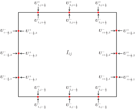
Refer to caption
Figure 3.1. The limiting values at Q𝑄Q Gaussian nodes on four edges of the cell Iijsubscript𝐼𝑖𝑗I_{ij} with Q=3𝑄3Q=3.

Let {x^iα}α=1Lsuperscriptsubscriptsuperscriptsubscript^𝑥𝑖𝛼𝛼1𝐿\{\hat{x}_{i}^{\alpha}\}_{\alpha=1}^{L} and {y^jα}α=1Lsuperscriptsubscriptsuperscriptsubscript^𝑦𝑗𝛼𝛼1𝐿\{\hat{y}_{j}^{\alpha}\}_{\alpha=1}^{L} be the Gauss-Lobatto nodes transformed into the intervals [xi12,xi+12]subscript𝑥𝑖12subscript𝑥𝑖12\left[x_{i-\frac{1}{2}},x_{i+\frac{1}{2}}\right] and [yj12,yj+12]subscript𝑦𝑗12subscript𝑦𝑗12\left[y_{j-\frac{1}{2}},y_{j+\frac{1}{2}}\right] respectively, and {ω^α}α=1Lsuperscriptsubscriptsubscript^𝜔𝛼𝛼1𝐿\{\hat{\omega}_{\alpha}\}_{\alpha=1}^{L} be associated weights satisfying α=1Lω^α=1superscriptsubscript𝛼1𝐿subscript^𝜔𝛼1\sum\limits_{\alpha=1}^{L}\hat{\omega}_{\alpha}=1. Here L(K+3)/2𝐿𝐾32L\geq(K+3)/2 such that the algebraic precision degree of corresponding quadrature is at least K𝐾K. Similar to Theorem 3.2 for the 1D case, we have the following sufficient conditions for that the high-order accurate scheme (3.19) is PCP.

Theorem 3.5.

If 𝐔ijn(x,y)=:(Dij(x,y),𝐦ij(x,y),𝐁ij(x,y),Eij(x,y)){\mbox{\boldmath\small$U$}}_{ij}^{n}(x,y)=:\big{(}D_{ij}(x,y),\mbox{\boldmath\small$m$}_{ij}(x,y),\mbox{\boldmath\small$B$}_{ij}(x,y),E_{ij}(x,y)\big{)}^{\top} satisfy:
(i). the discrete divergence-free conditions

divijin𝑩1Δxβ=1Qωβ((B1)i+12,β(B1)i12,β+)+1Δyβ=1Qωβ((B2)β,j+12(B2)β,j12+)=0,superscriptsubscriptdiv𝑖𝑗in𝑩1Δ𝑥superscriptsubscript𝛽1𝑄subscript𝜔𝛽superscriptsubscriptsubscript𝐵1𝑖12𝛽superscriptsubscriptsubscript𝐵1𝑖12𝛽1Δ𝑦superscriptsubscript𝛽1𝑄subscript𝜔𝛽superscriptsubscriptsubscript𝐵2𝛽𝑗12superscriptsubscriptsubscript𝐵2𝛽𝑗120\displaystyle\mbox{\rm div}_{ij}^{\mbox{\tiny\rm in}}{\mbox{\boldmath\small$B$}}\triangleq\frac{1}{\Delta x}\sum\limits_{\beta=1}^{Q}\omega_{\beta}\Big{(}(B_{1})_{i+\frac{1}{2},\beta}^{-}-(B_{1})_{i-\frac{1}{2},\beta}^{+}\Big{)}+\frac{1}{\Delta y}\sum\limits_{\beta=1}^{Q}\omega_{\beta}\Big{(}(B_{2})_{\beta,j+\frac{1}{2}}^{-}-(B_{2})_{\beta,j-\frac{1}{2}}^{+}\Big{)}=0, (3.20)
divijout𝑩1Δxβ=1Qωβ((B1)i+12,β+(B1)i12,β)+1Δyβ=1Qωβ((B2)β,j+12+(B2)β,j12)=0,superscriptsubscriptdiv𝑖𝑗out𝑩1Δ𝑥superscriptsubscript𝛽1𝑄subscript𝜔𝛽superscriptsubscriptsubscript𝐵1𝑖12𝛽superscriptsubscriptsubscript𝐵1𝑖12𝛽1Δ𝑦superscriptsubscript𝛽1𝑄subscript𝜔𝛽superscriptsubscriptsubscript𝐵2𝛽𝑗12superscriptsubscriptsubscript𝐵2𝛽𝑗120\displaystyle\mbox{\rm div}_{ij}^{\mbox{\tiny\rm out}}{\mbox{\boldmath\small$B$}}\triangleq\frac{1}{\Delta x}\sum\limits_{\beta=1}^{Q}\omega_{\beta}\Big{(}(B_{1})_{i+\frac{1}{2},\beta}^{+}-(B_{1})_{i-\frac{1}{2},\beta}^{-}\Big{)}+\frac{1}{\Delta y}\sum\limits_{\beta=1}^{Q}\omega_{\beta}\Big{(}(B_{2})_{\beta,j+\frac{1}{2}}^{+}-(B_{2})_{\beta,j-\frac{1}{2}}^{-}\Big{)}=0, (3.21)

for all i𝑖i and j𝑗j, and
(ii). 𝐔ijn(x^iα,yjβ),𝐔ijn(xiβ,y^jα)𝒢superscriptsubscript𝐔𝑖𝑗𝑛superscriptsubscript^𝑥𝑖𝛼superscriptsubscript𝑦𝑗𝛽superscriptsubscript𝐔𝑖𝑗𝑛superscriptsubscript𝑥𝑖𝛽superscriptsubscript^𝑦𝑗𝛼𝒢\mbox{\boldmath\small$U$}_{ij}^{n}(\hat{x}_{i}^{\alpha},y_{j}^{\beta}),\mbox{\boldmath\small$U$}_{ij}^{n}(x_{i}^{\beta},\hat{y}_{j}^{\alpha})\in{\mathcal{G}}, for all i,j,α,β𝑖𝑗𝛼𝛽i,j,\alpha,\beta,
then under the CFL type condition

0<ΔtnΔx+ΔtnΔyω^1,0Δsubscript𝑡𝑛Δ𝑥Δsubscript𝑡𝑛Δ𝑦subscript^𝜔10<\frac{\Delta t_{n}}{\Delta x}+\frac{\Delta t_{n}}{\Delta y}\leq\hat{\omega}_{1}, (3.22)

the solution 𝐔¯jn+1superscriptsubscript¯𝐔𝑗𝑛1\overline{\mbox{\boldmath\small$U$}}_{j}^{n+1} of the scheme (3.19) belongs to 𝒢𝒢{\mathcal{G}}.

Proof.

The exactness of the Gauss-Lobatto quadrature rule with L𝐿L nodes and the Gauss quadrature rule with Q𝑄Q nodes for the polynomials of degree K𝐾K yields

𝑼¯ijn=1ΔxΔyIij𝑼ijn(x,y)𝑑x𝑑y=1Δxxi12xi+12(β=1Qωβ𝑼ijn(x,yjβ))𝑑x=β=1Qωβ(1Δxxi12xi+12𝑼ijn(x,yjβ)𝑑x)=β=1Qωβ(α=1Lω^α𝑼ijn(x^iα,yjβ))=α=1Lβ=1Qω^αωβ𝑼ijn(x^iα,yjβ).superscriptsubscript¯𝑼𝑖𝑗𝑛1Δ𝑥Δ𝑦subscriptdouble-integralsubscript𝐼𝑖𝑗superscriptsubscript𝑼𝑖𝑗𝑛𝑥𝑦differential-d𝑥differential-d𝑦1Δ𝑥superscriptsubscriptsubscript𝑥𝑖12subscript𝑥𝑖12superscriptsubscript𝛽1𝑄subscript𝜔𝛽superscriptsubscript𝑼𝑖𝑗𝑛𝑥superscriptsubscript𝑦𝑗𝛽differential-d𝑥superscriptsubscript𝛽1𝑄subscript𝜔𝛽1Δ𝑥superscriptsubscriptsubscript𝑥𝑖12subscript𝑥𝑖12superscriptsubscript𝑼𝑖𝑗𝑛𝑥superscriptsubscript𝑦𝑗𝛽differential-d𝑥superscriptsubscript𝛽1𝑄subscript𝜔𝛽superscriptsubscript𝛼1𝐿subscript^𝜔𝛼superscriptsubscript𝑼𝑖𝑗𝑛superscriptsubscript^𝑥𝑖𝛼superscriptsubscript𝑦𝑗𝛽superscriptsubscript𝛼1𝐿superscriptsubscript𝛽1𝑄subscript^𝜔𝛼subscript𝜔𝛽superscriptsubscript𝑼𝑖𝑗𝑛superscriptsubscript^𝑥𝑖𝛼superscriptsubscript𝑦𝑗𝛽\begin{split}\overline{\mbox{\boldmath\small$U$}}_{ij}^{n}&=\frac{1}{\Delta x\Delta y}\iint_{I_{ij}}{\mbox{\boldmath\small$U$}}_{ij}^{n}(x,y)~{}dxdy=\frac{1}{\Delta x}\int_{x_{i-\frac{1}{2}}}^{x_{i+\frac{1}{2}}}\left(\sum\limits_{\beta=1}^{Q}\omega_{\beta}\mbox{\boldmath\small$U$}_{ij}^{n}\left(x,y_{j}^{\beta}\right)\right)dx\\ &=\sum\limits_{\beta=1}^{Q}\omega_{\beta}\left(\frac{1}{\Delta x}\int_{x_{i-\frac{1}{2}}}^{x_{i+\frac{1}{2}}}\mbox{\boldmath\small$U$}_{ij}^{n}\left(x,y_{j}^{\beta}\right)dx\right)=\sum\limits_{\beta=1}^{Q}\omega_{\beta}\left(\sum\limits_{\alpha=1}^{L}\hat{\omega}_{\alpha}\mbox{\boldmath\small$U$}_{ij}^{n}\left(\hat{x}_{i}^{\alpha},y_{j}^{\beta}\right)\right)\\ &=\sum\limits_{\alpha=1}^{L}\sum\limits_{\beta=1}^{Q}\hat{\omega}_{\alpha}\omega_{\beta}\mbox{\boldmath\small$U$}_{ij}^{n}\left(\hat{x}_{i}^{\alpha},y_{j}^{\beta}\right).\end{split} (3.23)

Similarly, one has

𝑼¯ijn=α=1Lβ=1Qω^αωβ𝑼ijn(xiβ,y^jα).superscriptsubscript¯𝑼𝑖𝑗𝑛superscriptsubscript𝛼1𝐿superscriptsubscript𝛽1𝑄subscript^𝜔𝛼subscript𝜔𝛽superscriptsubscript𝑼𝑖𝑗𝑛superscriptsubscript𝑥𝑖𝛽superscriptsubscript^𝑦𝑗𝛼\overline{\mbox{\boldmath\small$U$}}_{ij}^{n}=\sum\limits_{\alpha=1}^{L}\sum\limits_{\beta=1}^{Q}\hat{\omega}_{\alpha}\omega_{\beta}\mbox{\boldmath\small$U$}_{ij}^{n}\left(x_{i}^{\beta},\hat{y}_{j}^{\alpha}\right). (3.24)

By combining (3.23) and (3.24), and using 𝑼ijn(x^i1,yjβ)=𝑼i12,β+superscriptsubscript𝑼𝑖𝑗𝑛superscriptsubscript^𝑥𝑖1superscriptsubscript𝑦𝑗𝛽superscriptsubscript𝑼𝑖12𝛽\mbox{\boldmath\small$U$}_{ij}^{n}\left(\hat{x}_{i}^{1},y_{j}^{\beta}\right)=\mbox{\boldmath\small$U$}_{i-\frac{1}{2},\beta}^{+}, 𝑼ijn(x^iL,yjβ)=𝑼i+12,βsuperscriptsubscript𝑼𝑖𝑗𝑛superscriptsubscript^𝑥𝑖𝐿superscriptsubscript𝑦𝑗𝛽superscriptsubscript𝑼𝑖12𝛽\mbox{\boldmath\small$U$}_{ij}^{n}\left(\hat{x}_{i}^{L},y_{j}^{\beta}\right)=\mbox{\boldmath\small$U$}_{i+\frac{1}{2},\beta}^{-}, 𝑼ijn(xiβ,y^j1)=𝑼β,j12+superscriptsubscript𝑼𝑖𝑗𝑛superscriptsubscript𝑥𝑖𝛽superscriptsubscript^𝑦𝑗1superscriptsubscript𝑼𝛽𝑗12\mbox{\boldmath\small$U$}_{ij}^{n}\left(x_{i}^{\beta},\hat{y}_{j}^{1}\right)=\mbox{\boldmath\small$U$}_{\beta,j-\frac{1}{2}}^{+}, 𝑼ijn(xiβ,y^jL)=𝑼β,j+12superscriptsubscript𝑼𝑖𝑗𝑛superscriptsubscript𝑥𝑖𝛽superscriptsubscript^𝑦𝑗𝐿superscriptsubscript𝑼𝛽𝑗12\mbox{\boldmath\small$U$}_{ij}^{n}\left(x_{i}^{\beta},\hat{y}_{j}^{L}\right)=\mbox{\boldmath\small$U$}_{\beta,j+\frac{1}{2}}^{-}, and ω^1=ω^Lsubscript^𝜔1subscript^𝜔𝐿\hat{\omega}_{1}=\hat{\omega}_{L}, one has

𝑼¯ijnsuperscriptsubscript¯𝑼𝑖𝑗𝑛\displaystyle\overline{\mbox{\boldmath\small$U$}}_{ij}^{n} =λxλx+λy𝑼¯ijn+λyλx+λy𝑼¯ijnabsentsubscript𝜆𝑥subscript𝜆𝑥subscript𝜆𝑦superscriptsubscript¯𝑼𝑖𝑗𝑛subscript𝜆𝑦subscript𝜆𝑥subscript𝜆𝑦superscriptsubscript¯𝑼𝑖𝑗𝑛\displaystyle=\frac{\lambda_{x}}{\lambda_{x}+\lambda_{y}}\overline{\mbox{\boldmath\small$U$}}_{ij}^{n}+\frac{\lambda_{y}}{\lambda_{x}+\lambda_{y}}\overline{\mbox{\boldmath\small$U$}}_{ij}^{n}
=λxλx+λyα=1Lβ=1Qω^αωβ𝑼ijn(x^iα,yjβ)+λyλx+λyα=1Lβ=1Qω^αωβ𝑼ijn(xiβ,y^jα)absentsubscript𝜆𝑥subscript𝜆𝑥subscript𝜆𝑦superscriptsubscript𝛼1𝐿superscriptsubscript𝛽1𝑄subscript^𝜔𝛼subscript𝜔𝛽superscriptsubscript𝑼𝑖𝑗𝑛superscriptsubscript^𝑥𝑖𝛼superscriptsubscript𝑦𝑗𝛽subscript𝜆𝑦subscript𝜆𝑥subscript𝜆𝑦superscriptsubscript𝛼1𝐿superscriptsubscript𝛽1𝑄subscript^𝜔𝛼subscript𝜔𝛽superscriptsubscript𝑼𝑖𝑗𝑛superscriptsubscript𝑥𝑖𝛽superscriptsubscript^𝑦𝑗𝛼\displaystyle=\frac{\lambda_{x}}{\lambda_{x}+\lambda_{y}}\sum\limits_{\alpha=1}^{L}\sum\limits_{\beta=1}^{Q}\hat{\omega}_{\alpha}\omega_{\beta}\mbox{\boldmath\small$U$}_{ij}^{n}\left(\hat{x}_{i}^{\alpha},y_{j}^{\beta}\right)+\frac{\lambda_{y}}{\lambda_{x}+\lambda_{y}}\sum\limits_{\alpha=1}^{L}\sum\limits_{\beta=1}^{Q}\hat{\omega}_{\alpha}\omega_{\beta}\mbox{\boldmath\small$U$}_{ij}^{n}\left(x_{i}^{\beta},\hat{y}_{j}^{\alpha}\right)
=λxλx+λyα=2L1β=1Qω^αωβ𝑼ijn(x^iα,yjβ)+λyλx+λyα=2L1β=1Qω^αωβ𝑼ijn(xiβ,y^jα)+λxω^1λx+λyβ=1Qωβ(𝑼i12,β++𝑼i+12,β)+λyω^1λx+λyβ=1Qωβ(𝑼β,j12++𝑼β,j+12),absentsubscript𝜆𝑥subscript𝜆𝑥subscript𝜆𝑦superscriptsubscript𝛼2𝐿1superscriptsubscript𝛽1𝑄subscript^𝜔𝛼subscript𝜔𝛽superscriptsubscript𝑼𝑖𝑗𝑛superscriptsubscript^𝑥𝑖𝛼superscriptsubscript𝑦𝑗𝛽subscript𝜆𝑦subscript𝜆𝑥subscript𝜆𝑦superscriptsubscript𝛼2𝐿1superscriptsubscript𝛽1𝑄subscript^𝜔𝛼subscript𝜔𝛽superscriptsubscript𝑼𝑖𝑗𝑛superscriptsubscript𝑥𝑖𝛽superscriptsubscript^𝑦𝑗𝛼subscript𝜆𝑥subscript^𝜔1subscript𝜆𝑥subscript𝜆𝑦superscriptsubscript𝛽1𝑄subscript𝜔𝛽superscriptsubscript𝑼𝑖12𝛽superscriptsubscript𝑼𝑖12𝛽subscript𝜆𝑦subscript^𝜔1subscript𝜆𝑥subscript𝜆𝑦superscriptsubscript𝛽1𝑄subscript𝜔𝛽superscriptsubscript𝑼𝛽𝑗12superscriptsubscript𝑼𝛽𝑗12\displaystyle\begin{split}&=\frac{\lambda_{x}}{\lambda_{x}+\lambda_{y}}\sum\limits_{\alpha=2}^{L-1}\sum\limits_{\beta=1}^{Q}\hat{\omega}_{\alpha}\omega_{\beta}\mbox{\boldmath\small$U$}_{ij}^{n}\left(\hat{x}_{i}^{\alpha},y_{j}^{\beta}\right)+\frac{\lambda_{y}}{\lambda_{x}+\lambda_{y}}\sum\limits_{\alpha=2}^{L-1}\sum\limits_{\beta=1}^{Q}\hat{\omega}_{\alpha}\omega_{\beta}\mbox{\boldmath\small$U$}_{ij}^{n}\left(x_{i}^{\beta},\hat{y}_{j}^{\alpha}\right)\\ &\quad+\frac{\lambda_{x}\hat{\omega}_{1}}{\lambda_{x}+\lambda_{y}}\sum\limits_{\beta=1}^{Q}\omega_{\beta}\left(\mbox{\boldmath\small$U$}_{i-\frac{1}{2},\beta}^{+}+\mbox{\boldmath\small$U$}_{i+\frac{1}{2},\beta}^{-}\right)+\frac{\lambda_{y}\hat{\omega}_{1}}{\lambda_{x}+\lambda_{y}}\sum\limits_{\beta=1}^{Q}\omega_{\beta}\left(\mbox{\boldmath\small$U$}_{\beta,j-\frac{1}{2}}^{+}+\mbox{\boldmath\small$U$}_{\beta,j+\frac{1}{2}}^{-}\right),\end{split}

where λx:=Δtn/Δxassignsubscript𝜆𝑥Δsubscript𝑡𝑛Δ𝑥\lambda_{x}:=\Delta t_{n}/\Delta x and λy:=Δtn/Δyassignsubscript𝜆𝑦Δsubscript𝑡𝑛Δ𝑦\lambda_{y}:=\Delta t_{n}/\Delta y. Substituting the above identity and (3.2) into (3.19) gives

𝑼¯ijn+1=λxλx+λyα=2L1β=1Qω^αωβ𝑼ijn(x^iα,yjβ)+λyλx+λyα=2L1β=1Qω^αωβ𝑼ijn(xiβ,y^jα)+λxω^1λx+λyβ=1Qωβ(𝑼i12,β++𝑼i+12,β)+λyω^1λx+λyβ=1Qωβ(𝑼β,j12++𝑼β,j+12)λxβ=1Qωβ(𝑭^1(𝑼i+12,β,𝑼i+12,β+)𝑭^1(𝑼i12,β,𝑼i12,β+))λyβ=1Qωβ(𝑭^2(𝑼β,j+12,𝑼β,j+12+)𝑭^2(𝑼β,j12,𝑼β,j12+))superscriptsubscript¯𝑼𝑖𝑗𝑛1subscript𝜆𝑥subscript𝜆𝑥subscript𝜆𝑦superscriptsubscript𝛼2𝐿1superscriptsubscript𝛽1𝑄subscript^𝜔𝛼subscript𝜔𝛽superscriptsubscript𝑼𝑖𝑗𝑛superscriptsubscript^𝑥𝑖𝛼superscriptsubscript𝑦𝑗𝛽subscript𝜆𝑦subscript𝜆𝑥subscript𝜆𝑦superscriptsubscript𝛼2𝐿1superscriptsubscript𝛽1𝑄subscript^𝜔𝛼subscript𝜔𝛽superscriptsubscript𝑼𝑖𝑗𝑛superscriptsubscript𝑥𝑖𝛽superscriptsubscript^𝑦𝑗𝛼subscript𝜆𝑥subscript^𝜔1subscript𝜆𝑥subscript𝜆𝑦superscriptsubscript𝛽1𝑄subscript𝜔𝛽superscriptsubscript𝑼𝑖12𝛽superscriptsubscript𝑼𝑖12𝛽subscript𝜆𝑦subscript^𝜔1subscript𝜆𝑥subscript𝜆𝑦superscriptsubscript𝛽1𝑄subscript𝜔𝛽superscriptsubscript𝑼𝛽𝑗12superscriptsubscript𝑼𝛽𝑗12subscript𝜆𝑥superscriptsubscript𝛽1𝑄subscript𝜔𝛽subscriptbold-^𝑭1subscriptsuperscript𝑼𝑖12𝛽subscriptsuperscript𝑼𝑖12𝛽subscriptbold-^𝑭1subscriptsuperscript𝑼𝑖12𝛽subscriptsuperscript𝑼𝑖12𝛽subscript𝜆𝑦superscriptsubscript𝛽1𝑄subscript𝜔𝛽subscriptbold-^𝑭2subscriptsuperscript𝑼𝛽𝑗12subscriptsuperscript𝑼𝛽𝑗12subscriptbold-^𝑭2subscriptsuperscript𝑼𝛽𝑗12subscriptsuperscript𝑼𝛽𝑗12\displaystyle\begin{split}\overline{\mbox{\boldmath\small$U$}}_{ij}^{n+1}&=\frac{\lambda_{x}}{\lambda_{x}+\lambda_{y}}\sum\limits_{\alpha=2}^{L-1}\sum\limits_{\beta=1}^{Q}\hat{\omega}_{\alpha}\omega_{\beta}\mbox{\boldmath\small$U$}_{ij}^{n}\left(\hat{x}_{i}^{\alpha},y_{j}^{\beta}\right)+\frac{\lambda_{y}}{\lambda_{x}+\lambda_{y}}\sum\limits_{\alpha=2}^{L-1}\sum\limits_{\beta=1}^{Q}\hat{\omega}_{\alpha}\omega_{\beta}\mbox{\boldmath\small$U$}_{ij}^{n}\left(x_{i}^{\beta},\hat{y}_{j}^{\alpha}\right)\\ &\quad+\frac{\lambda_{x}\hat{\omega}_{1}}{\lambda_{x}+\lambda_{y}}\sum\limits_{\beta=1}^{Q}\omega_{\beta}\left(\mbox{\boldmath\small$U$}_{i-\frac{1}{2},\beta}^{+}+\mbox{\boldmath\small$U$}_{i+\frac{1}{2},\beta}^{-}\right)+\frac{\lambda_{y}\hat{\omega}_{1}}{\lambda_{x}+\lambda_{y}}\sum\limits_{\beta=1}^{Q}\omega_{\beta}\left(\mbox{\boldmath\small$U$}_{\beta,j-\frac{1}{2}}^{+}+\mbox{\boldmath\small$U$}_{\beta,j+\frac{1}{2}}^{-}\right)\\ &\quad-\lambda_{x}\sum\limits_{\beta=1}^{Q}\omega_{\beta}\bigg{(}\mbox{\boldmath\small$\hat{F}$}_{1}(\mbox{\boldmath\small$U$}^{-}_{i+\frac{1}{2},\beta},{\mbox{\boldmath\small$U$}}^{+}_{i+\frac{1}{2},\beta})-\mbox{\boldmath\small$\hat{F}$}_{1}({\mbox{\boldmath\small$U$}}^{-}_{i-\frac{1}{2},\beta},\mbox{\boldmath\small$U$}^{+}_{i-\frac{1}{2},\beta})\bigg{)}\\ &\quad-\lambda_{y}\sum\limits_{\beta=1}^{Q}\omega_{\beta}\bigg{(}\mbox{\boldmath\small$\hat{F}$}_{2}(\mbox{\boldmath\small$U$}^{-}_{\beta,j+\frac{1}{2}},{\mbox{\boldmath\small$U$}}^{+}_{\beta,j+\frac{1}{2}})-\mbox{\boldmath\small$\hat{F}$}_{2}({\mbox{\boldmath\small$U$}}^{-}_{\beta,j-\frac{1}{2}},\mbox{\boldmath\small$U$}^{+}_{\beta,j-\frac{1}{2}})\bigg{)}\end{split}
=(12ω^1)Ξ1+(λx+λy)Ξ2+(2ω^1(λx+λy))Ξ3,absent12subscript^𝜔1subscriptΞ1subscript𝜆𝑥subscript𝜆𝑦subscriptΞ22subscript^𝜔1subscript𝜆𝑥subscript𝜆𝑦subscriptΞ3\displaystyle=(1-2\hat{\omega}_{1})\Xi_{1}+\left(\lambda_{x}+\lambda_{y}\right)\Xi_{2}+\big{(}2\hat{\omega}_{1}-\left(\lambda_{x}+\lambda_{y}\right)\big{)}\Xi_{3}, (3.25)

with

Ξ1subscriptΞ1\displaystyle\Xi_{1} :=α=2L1ω^α12ω^1[λxλx+λyβ=1Qωβ𝑼ij(x^iα,yjβ)+λyλx+λyβ=1Qωβ𝑼ij(xiβ,y^jα)],assignabsentsuperscriptsubscript𝛼2𝐿1subscript^𝜔𝛼12subscript^𝜔1delimited-[]subscript𝜆𝑥subscript𝜆𝑥subscript𝜆𝑦superscriptsubscript𝛽1𝑄subscript𝜔𝛽subscript𝑼𝑖𝑗superscriptsubscript^𝑥𝑖𝛼superscriptsubscript𝑦𝑗𝛽subscript𝜆𝑦subscript𝜆𝑥subscript𝜆𝑦superscriptsubscript𝛽1𝑄subscript𝜔𝛽subscript𝑼𝑖𝑗superscriptsubscript𝑥𝑖𝛽superscriptsubscript^𝑦𝑗𝛼\displaystyle:=\sum\limits_{\alpha=2}^{L-1}\frac{\hat{\omega}_{\alpha}}{1-2\hat{\omega}_{1}}\left[\frac{\lambda_{x}}{\lambda_{x}+\lambda_{y}}\sum\limits_{\beta=1}^{Q}\omega_{\beta}\mbox{\boldmath\small$U$}_{ij}\left(\hat{x}_{i}^{\alpha},y_{j}^{\beta}\right)+\frac{\lambda_{y}}{\lambda_{x}+\lambda_{y}}\sum\limits_{\beta=1}^{Q}\omega_{\beta}\mbox{\boldmath\small$U$}_{ij}\left(x_{i}^{\beta},\hat{y}_{j}^{\alpha}\right)\right],
Ξ2:=12(1Δx+1Δy)β=1Qωβ[1Δx(𝑼i+12,β+𝑭1(𝑼i+12,β+)+𝑼i12,β+𝑭1(𝑼i12,β))+1Δy(𝑼β,j+12+𝑭2(𝑼β,j+12+)+𝑼β,j12+𝑭2(𝑼β,j12))],assignsubscriptΞ2121Δ𝑥1Δ𝑦superscriptsubscript𝛽1𝑄subscript𝜔𝛽delimited-[]1Δ𝑥superscriptsubscript𝑼𝑖12𝛽subscript𝑭1superscriptsubscript𝑼𝑖12𝛽superscriptsubscript𝑼𝑖12𝛽subscript𝑭1superscriptsubscript𝑼𝑖12𝛽1Δ𝑦superscriptsubscript𝑼𝛽𝑗12subscript𝑭2superscriptsubscript𝑼𝛽𝑗12superscriptsubscript𝑼𝛽𝑗12subscript𝑭2superscriptsubscript𝑼𝛽𝑗12\displaystyle\begin{split}\Xi_{2}&:=\frac{1}{2\left(\frac{1}{\Delta x}+\frac{1}{\Delta y}\right)}\sum\limits_{\beta=1}^{Q}{{\omega_{\beta}}}\bigg{[}\frac{1}{\Delta x}\bigg{(}{\mbox{\boldmath\small$U$}}_{i+\frac{1}{2},\beta}^{+}-\mbox{\boldmath\small$F$}_{1}\left({\mbox{\boldmath\small$U$}}_{i+\frac{1}{2},\beta}^{+}\right)+{\mbox{\boldmath\small$U$}}_{i-\frac{1}{2},\beta}^{-}+\mbox{\boldmath\small$F$}_{1}\left({\mbox{\boldmath\small$U$}}_{i-\frac{1}{2},\beta}^{-}\right)\bigg{)}\\ &\quad+\frac{1}{\Delta y}\bigg{(}{\mbox{\boldmath\small$U$}}_{\beta,j+\frac{1}{2}}^{+}-\mbox{\boldmath\small$F$}_{2}\left({\mbox{\boldmath\small$U$}}_{\beta,j+\frac{1}{2}}^{+}\right)+{\mbox{\boldmath\small$U$}}_{\beta,j-\frac{1}{2}}^{-}+\mbox{\boldmath\small$F$}_{2}\left({\mbox{\boldmath\small$U$}}_{\beta,j-\frac{1}{2}}^{-}\right)\bigg{)}\bigg{]},\end{split}
Ξ3:=12(1Δx+1Δy)β=1Qωβ[1Δx(𝑼i+12,βθ1𝑭1(𝑼i+12,β)+𝑼i12,β++θ1𝑭1(𝑼i12,β+))+1Δy(𝑼β,j+12θ1𝑭2(𝑼β,j+12)+𝑼β,j12++θ1𝑭2(𝑼β,j12+))],assignsubscriptΞ3121Δ𝑥1Δ𝑦superscriptsubscript𝛽1𝑄subscript𝜔𝛽delimited-[]1Δ𝑥superscriptsubscript𝑼𝑖12𝛽superscript𝜃1subscript𝑭1superscriptsubscript𝑼𝑖12𝛽superscriptsubscript𝑼𝑖12𝛽superscript𝜃1subscript𝑭1superscriptsubscript𝑼𝑖12𝛽1Δ𝑦superscriptsubscript𝑼𝛽𝑗12superscript𝜃1subscript𝑭2superscriptsubscript𝑼𝛽𝑗12superscriptsubscript𝑼𝛽𝑗12superscript𝜃1subscript𝑭2superscriptsubscript𝑼𝛽𝑗12\displaystyle\begin{split}\Xi_{3}&:=\frac{1}{2\left(\frac{1}{\Delta x}+\frac{1}{\Delta y}\right)}\sum\limits_{\beta=1}^{Q}{{\omega_{\beta}}}\bigg{[}\frac{1}{\Delta x}\bigg{(}{\mbox{\boldmath\small$U$}}_{i+\frac{1}{2},\beta}^{-}-\theta^{-1}\mbox{\boldmath\small$F$}_{1}\left({\mbox{\boldmath\small$U$}}_{i+\frac{1}{2},\beta}^{-}\right)+{\mbox{\boldmath\small$U$}}_{i-\frac{1}{2},\beta}^{+}+\theta^{-1}\mbox{\boldmath\small$F$}_{1}\left({\mbox{\boldmath\small$U$}}_{i-\frac{1}{2},\beta}^{+}\right)\bigg{)}\\ &\quad+\frac{1}{\Delta y}\bigg{(}{\mbox{\boldmath\small$U$}}_{\beta,j+\frac{1}{2}}^{-}-\theta^{-1}\mbox{\boldmath\small$F$}_{2}\left({\mbox{\boldmath\small$U$}}_{\beta,j+\frac{1}{2}}^{-}\right)+{\mbox{\boldmath\small$U$}}_{\beta,j-\frac{1}{2}}^{+}+\theta^{-1}\mbox{\boldmath\small$F$}_{2}\left({\mbox{\boldmath\small$U$}}_{\beta,j-\frac{1}{2}}^{+}\right)\bigg{)}\bigg{]},\end{split}

where θ:=2ω^1λx+λy11assign𝜃2subscript^𝜔1subscript𝜆𝑥subscript𝜆𝑦11\theta:=\frac{2\hat{\omega}_{1}}{\lambda_{x}+\lambda_{y}}-1\geq 1. Thanks to the convexity of 𝒢𝒢\mathcal{G} and the condition (ii), Ξ1𝒢subscriptΞ1𝒢\Xi_{1}\in{\mathcal{G}}. With 𝑼i±12,β,𝑼β,j±12𝒢superscriptsubscript𝑼plus-or-minus𝑖12𝛽minus-or-plussuperscriptsubscript𝑼𝛽plus-or-minus𝑗12minus-or-plus𝒢{\mbox{\boldmath\small$U$}}_{i\pm\frac{1}{2},\beta}^{\mp},{\mbox{\boldmath\small$U$}}_{\beta,j\pm\frac{1}{2}}^{\mp}\in{\mathcal{G}}, θ1𝜃1\theta\geq 1, and the condition (3.20), one has Ξ3𝒢subscriptΞ3𝒢\Xi_{3}\in{\mathcal{G}} by the generalized LxF splitting property in Theorem 2.5. Similarly, utilizing the condition (3.21) gives Ξ2𝒢subscriptΞ2𝒢\Xi_{2}\in{\mathcal{G}}. Thus using (3.25) and the convexity of 𝒢𝒢\mathcal{G} yields 𝑼¯ijn+1𝒢superscriptsubscript¯𝑼𝑖𝑗𝑛1𝒢\overline{\mbox{\boldmath\small$U$}}_{ij}^{n+1}\in{\mathcal{G}}, and completes the proof. ∎

Remark 3.2.

Both (3.20) or (3.21) in the condition (i) are approximating (2.44) by replacing x0subscript𝑥0x_{0} and y0subscript𝑦0y_{0} with xi12subscript𝑥𝑖12x_{i-\frac{1}{2}} and yj12subscript𝑦𝑗12y_{j-\frac{1}{2}} respectively.

Remark 3.3.

For some high-order finite volume methods, it only needs to reconstruct the limiting values 𝐔i12,β+superscriptsubscript𝐔𝑖12𝛽\mbox{\boldmath\small$U$}_{i-\frac{1}{2},\beta}^{+}, 𝐔i+12,βsuperscriptsubscript𝐔𝑖12𝛽\mbox{\boldmath\small$U$}_{i+\frac{1}{2},\beta}^{-}, 𝐔β,j12+superscriptsubscript𝐔𝛽𝑗12\mbox{\boldmath\small$U$}_{\beta,j-\frac{1}{2}}^{+}, 𝐔β,j+12superscriptsubscript𝐔𝛽𝑗12\mbox{\boldmath\small$U$}_{\beta,j+\frac{1}{2}}^{-}, instead of the polynomial vector 𝐔ijn(x,y)superscriptsubscript𝐔𝑖𝑗𝑛𝑥𝑦{\mbox{\boldmath\small$U$}}_{ij}^{n}(x,y). In this case, the condition (ii) in Theorem 3.5 can be replaced with the following condition

𝑼i12,β+,𝑼i+12,β,𝑼β,j12+,𝑼β,j+12𝒢,β=1,2,,Q,Ξ1=112ω^1(𝑼¯ijnω^1β=1Qωβλx+λy(λx(𝑼i12,β++𝑼i+12,β)+λy(𝑼β,j12++𝑼β,j+12)))𝒢,\begin{split}&\mbox{\boldmath\small$U$}_{i-\frac{1}{2},\beta}^{+},\mbox{\boldmath\small$U$}_{i+\frac{1}{2},\beta}^{-},\mbox{\boldmath\small$U$}_{\beta,j-\frac{1}{2}}^{+},\mbox{\boldmath\small$U$}_{\beta,j+\frac{1}{2}}^{-}\in{\mathcal{G}},\quad\beta=1,2,\cdots,Q,\\ &\Xi_{1}=\frac{1}{1-2\hat{\omega}_{1}}\Bigg{(}\overline{\mbox{\boldmath\small$U$}}_{ij}^{n}-\hat{\omega}_{1}\sum\limits_{\beta=1}^{Q}\frac{\omega_{\beta}}{{\lambda_{x}+\lambda_{y}}}\bigg{(}\lambda_{x}\Big{(}\mbox{\boldmath\small$U$}_{i-\frac{1}{2},\beta}^{+}+\mbox{\boldmath\small$U$}_{i+\frac{1}{2},\beta}^{-}\Big{)}+\lambda_{y}\Big{(}\mbox{\boldmath\small$U$}_{\beta,j-\frac{1}{2}}^{+}+\mbox{\boldmath\small$U$}_{\beta,j+\frac{1}{2}}^{-}\Big{)}\bigg{)}\Bigg{)}\in{\mathcal{G}},\end{split}

for all i𝑖i and j𝑗j.

It is worth emphasizing the above discussions can be extended to non-uniform or unstructured meshes by using Theorem 2.7. Theorem 3.5 provides two sufficient conditions (i) and (ii) on the function 𝑼ijn(x,y)superscriptsubscript𝑼𝑖𝑗𝑛𝑥𝑦\mbox{\boldmath\small$U$}_{ij}^{n}(x,y) reconstructed in the finite volume method or evolved in the DG method in order to ensure that the numerical schemes (3.19) is PCP. The condition (ii) can be easily met by using the PCP limiter similar to that in Section 3.1.2, but Eqs. (3.20) and (3.21) in the condition (i) are two constraints on the discrete divergence. By using the divergence theorem, it can be seen that the discrete divergence-free condition (3.20) may be met if the the reconstructed or evolved polynomial vector (B1,B2)ij(x,y)subscriptsubscript𝐵1subscript𝐵2𝑖𝑗𝑥𝑦(B_{1},B_{2})_{ij}(x,y) is locally divergence-free, see e.g. [28, 47]. The locally divergence-free property of (B1,B2)ij(x,y)subscriptsubscript𝐵1subscript𝐵2𝑖𝑗𝑥𝑦(B_{1},B_{2})_{ij}(x,y) is not destroyed in the PCP limiting procedure since the PCP limiter modifies the vectors 𝑼ijn(x,y)superscriptsubscript𝑼𝑖𝑗𝑛𝑥𝑦\mbox{\boldmath\small$U$}_{ij}^{n}(x,y) only with a simple scaling. The condition (3.21) is necessary for a PCP numerical scheme for the RMHD equations, see Example 3.1, where the magnetic vector satisfies (3.20) and the condition (ii). Numerical results in Section 4 will further demonstrate the importance of condition (3.21). However, it is not easy to meet the condition (3.21) because (3.21) depends on the limiting values of the magnetic field calculated from the neighboring cells Ii±1,jsubscript𝐼plus-or-minus𝑖1𝑗I_{i\pm 1,j} and Ii,j±1subscript𝐼𝑖plus-or-minus𝑗1I_{i,j\pm 1} of Iijsubscript𝐼𝑖𝑗I_{ij}. If the polynomials (B1,B2)ij(x,y)subscriptsubscript𝐵1subscript𝐵2𝑖𝑗𝑥𝑦(B_{1},B_{2})_{ij}(x,y) are globally or exactly divergence-free, in other words, it is locally divergence-free in Iijsubscript𝐼𝑖𝑗I_{ij} with normal magnetic component continuous across the cell interface, then (3.20) and (3.21) are satisfied. But the PCP limiter with local scaling may destroy the globally or exactly divergence-free property of (B1,B2)ij(x,y)subscriptsubscript𝐵1subscript𝐵2𝑖𝑗𝑥𝑦(B_{1},B_{2})_{ij}(x,y). Hence, it is nontrivial and still open to design a limiting procedure for the polynomial vector 𝑼ijn(x,y)superscriptsubscript𝑼𝑖𝑗𝑛𝑥𝑦\mbox{\boldmath\small$U$}_{ij}^{n}(x,y) satisfying two sufficient conditions in Theorem 3.5 at the same time.

Remark 3.4.

As the mesh is refined, it can be weakened that violating the condition (3.21) impacts on the PCP property, if the reconstructed or evolved polynomial vector (B1,B2)ij(x,y)subscriptsubscript𝐵1subscript𝐵2𝑖𝑗𝑥𝑦(B_{1},B_{2})_{ij}(x,y) is locally divergence-free, i.e. divijin𝐁=0superscriptsubscriptdiv𝑖𝑗in𝐁0\mbox{\rm div}_{ij}^{\mbox{\tiny\rm in}}{\mbox{\boldmath\small$B$}}=0. In fact, the proof of Theorem 3.5 shows that the condition (3.21) is only related to Ξ2𝒢subscriptΞ2𝒢\Xi_{2}\in{\mathcal{G}}. If assuming that (B1,B2)ij(x,y)subscriptsubscript𝐵1subscript𝐵2𝑖𝑗𝑥𝑦(B_{1},B_{2})_{ij}(x,y) approximates the exact solution (B1,B2)(x,y,tn)subscript𝐵1subscript𝐵2𝑥𝑦subscript𝑡𝑛(B_{1},B_{2})(x,y,t_{n}) with at least first order, then the continuity of B1(x,y,tn)subscript𝐵1𝑥𝑦subscript𝑡𝑛B_{1}(x,y,t_{n}) across the edge {xi+12}×(yj12,yj+12)subscript𝑥𝑖12subscript𝑦𝑗12subscript𝑦𝑗12\big{\{}x_{i+\frac{1}{2}}\big{\}}\times\big{(}y_{j-\frac{1}{2}},y_{j+\frac{1}{2}}\big{)} implies

(B1)i+12,β=B1(xi+12,yjβ,tn)+𝒪(Δ),(B1)i+12,β+=B1(xi+12,yjβ,tn)+𝒪(Δ),formulae-sequencesuperscriptsubscriptsubscript𝐵1𝑖12𝛽subscript𝐵1subscript𝑥𝑖12superscriptsubscript𝑦𝑗𝛽subscript𝑡𝑛𝒪Δsuperscriptsubscriptsubscript𝐵1𝑖12𝛽subscript𝐵1subscript𝑥𝑖12superscriptsubscript𝑦𝑗𝛽subscript𝑡𝑛𝒪Δ(B_{1})_{i+\frac{1}{2},\beta}^{-}=B_{1}\big{(}x_{i+\frac{1}{2}},y_{j}^{\beta},t_{n}\big{)}+{\mathcal{O}}(\Delta),\quad(B_{1})_{i+\frac{1}{2},\beta}^{+}=B_{1}\big{(}x_{i+\frac{1}{2}},y_{j}^{\beta},t_{n}\big{)}+{\mathcal{O}}(\Delta),

where Δ=min{Δx,Δy}ΔΔ𝑥Δ𝑦\Delta=\min\{\Delta x,\Delta y\}. Similarly, one has

(B2)β,j+12=B2(xiβ,yj+12,tn)+𝒪(Δ),(B2)β,j+12=B2(xiβ,yj+12,tn)+𝒪(Δ).formulae-sequencesuperscriptsubscriptsubscript𝐵2𝛽𝑗12subscript𝐵2superscriptsubscript𝑥𝑖𝛽subscript𝑦𝑗12subscript𝑡𝑛𝒪Δsuperscriptsubscriptsubscript𝐵2𝛽𝑗12subscript𝐵2superscriptsubscript𝑥𝑖𝛽subscript𝑦𝑗12subscript𝑡𝑛𝒪Δ(B_{2})_{\beta,j+\frac{1}{2}}^{-}=B_{2}\big{(}x_{i}^{\beta},y_{j+\frac{1}{2}},t_{n}\big{)}+{\mathcal{O}}(\Delta),\quad(B_{2})_{\beta,j+\frac{1}{2}}^{-}=B_{2}\big{(}x_{i}^{\beta},y_{j+\frac{1}{2}},t_{n}\big{)}+{\mathcal{O}}(\Delta).

It follows that divijout𝐁=divijin𝐁+𝒪(1)=𝒪(1)superscriptsubscriptdiv𝑖𝑗out𝐁superscriptsubscriptdiv𝑖𝑗in𝐁𝒪1𝒪1\mbox{\rm div}_{ij}^{\mbox{\tiny\rm out}}{\mbox{\boldmath\small$B$}}=\mbox{\rm div}_{ij}^{\mbox{\tiny\rm in}}{\mbox{\boldmath\small$B$}}+{\mathcal{O}}(1)={\mathcal{O}}(1), so that Ξ2subscriptΞ2\Xi_{2} may not belong to 𝒢𝒢{\mathcal{G}}. However, Ξ2subscriptΞ2\Xi_{2} is very close to 𝒢𝒢{\mathcal{G}} in the sense of that the first component of Ξ2subscriptΞ2\Xi_{2} is positive, and for any 𝐁,𝐯3superscript𝐁superscript𝐯superscript3{\mbox{\boldmath\small$B$}}^{*},\mbox{\boldmath\small$v$}^{*}\in\mathbb{R}^{3} with |𝐯|<1superscript𝐯1|\mbox{\boldmath\small$v$}^{*}|<1, it holds

Ξ2𝒏+pm𝒗𝑩2(1Δx+1Δy)(divijout𝑩)=𝒪(Δ),subscriptΞ2superscript𝒏superscriptsubscript𝑝𝑚superscript𝒗superscript𝑩21Δ𝑥1Δ𝑦superscriptsubscriptdiv𝑖𝑗out𝑩𝒪Δ\Xi_{2}\cdot\mbox{\boldmath\small$n$}^{*}+p_{m}^{*}\geq-\frac{\mbox{\boldmath\small$v$}^{*}\cdot\mbox{\boldmath\small$B$}^{*}}{2\left(\frac{1}{\Delta x}+\frac{1}{\Delta y}\right)}\Big{(}\mbox{\rm div}_{ij}^{\mbox{\tiny\rm out}}{\mbox{\boldmath\small$B$}}\Big{)}=-{\mathcal{O}}(\Delta),

whose derivation is similar to that of Theorem 2.5. Therefore, as ΔΔ\Delta approaches 00, the convex combination in (3.25) becomes more possibly in 𝒢𝒢{\mathcal{G}}.

4. Numerical experiments

This section conducts numerical experiments on several 1D and 2D challenging RMHD problems with either large Lorentz factors, strong discontinuities, low plasma-beta β:=p/pmassign𝛽𝑝subscript𝑝𝑚\beta:=p/p_{m}, or low rest-mass density or pressure, to demonstrate our theoretical analyses and the performance of the proposed PCP limiter. Without loss of generality, we take the (third-order accurate) 2superscript2{\mathbb{P}}^{2}-based, locally divergence-free DG methods [47], together with the third-order SSP Runge-Kutta time disretization (3.10), as our base schemes. According to the analysis in Section 3.1.2, the 1D base scheme with the proposed PCP limiter results in a PCP DG scheme. As discussed in Section 3.2.2, the 2D base scheme with such limiter may not be PCP in general, because the discrete divergence-free condition (3.21) in Theorem 3.5 is not strictly satisfied even though the locally divergence-free property can ensure the condition (3.20). However, it will be shown in the following that the PCP limiter can still improve the robustness of 2D DG method. To meet the conditions (3.5) and (3.22), the time step-sizes in 1D and 2D will be taken as 0.15Δx0.15Δ𝑥0.15\Delta x and 0.15(1/Δx+1/Δy)10.15superscript1Δ𝑥1Δ𝑦10.15\left({1}/{\Delta x}+{1}/{\Delta y}\right)^{-1}, respectively. Unless otherwise stated, all the computations are restricted to the equation of state (2.1) with the adiabatic index Γ=5/3Γ53\Gamma=5/3.

Example 4.1 (Smooth problems).

A 1D and a 2D smooth problems are respectively solved within the domain [0,1]dsuperscript01𝑑[0,1]^{d} on the uniform meshes of Ndsuperscript𝑁𝑑N^{d} cells to test the accuracy of the 2superscript2{\mathbb{P}}^{2}-based DG methods with the proposed PCP limiter.

The 1D problem describes Alfvén waves propagating periodically with large velocity of 0.99 and low pressure, and has the exact solution

𝑽(x,t)=(1,0,v2,v3,1,κv2,κv3,102),(x,t)[0,1]×+,formulae-sequence𝑽𝑥𝑡superscript10subscript𝑣2subscript𝑣31𝜅subscript𝑣2𝜅subscript𝑣3superscript102top𝑥𝑡01superscript\mbox{\boldmath\small$V$}(x,t)=\big{(}1,0,v_{2},v_{3},1,\kappa v_{2},\kappa v_{3},10^{-2}\big{)}^{\top},\quad(x,t)\in[0,1]\times{\mathbb{R}}^{+},

where v2=0.99sin(2π(x+t/κ))subscript𝑣20.992𝜋𝑥𝑡𝜅v_{2}=0.99\sin(2\pi\big{(}x+t/\kappa)\big{)}, v3=0.99cos(2π(x+t/κ))subscript𝑣30.992𝜋𝑥𝑡𝜅v_{3}=0.99\cos(2\pi\big{(}x+t/\kappa)\big{)}, and κ=1+ρhW2𝜅1𝜌superscript𝑊2\kappa=\sqrt{1+\rho hW^{2}}. While the 2D problem’s exact solution is given by

𝑽(x,y,t)=(1+0.99999999sin(2π(x+y)),0.9,0.2,0,1,1,1,102),(x,y,t)[0,1]2×+,formulae-sequence𝑽𝑥𝑦𝑡superscript10.999999992𝜋𝑥𝑦0.90.20111superscript102top𝑥𝑦𝑡superscript012superscript\mbox{\boldmath\small$V$}(x,y,t)=\big{(}1+0.99999999\sin\big{(}2\pi(x+y)\big{)},0.9,0.2,0,1,1,1,10^{-2}\big{)}^{\top},\quad(x,y,t)\in[0,1]^{2}\times{\mathbb{R}}^{+},

which describes a RMHD sine wave fast propagating with low density and pressure.

Fig. 4.1 displays the l1superscript𝑙1l^{1}- and l2superscript𝑙2l^{2}-errors at t=1𝑡1t=1 and corresponding orders obtained by using the proposed DG methods, respectively. The results show that the theoretical orders are obtained in both 1D and 2D cases, and the PCP limiting procedure does not destroy the accuracy.
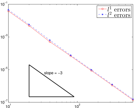
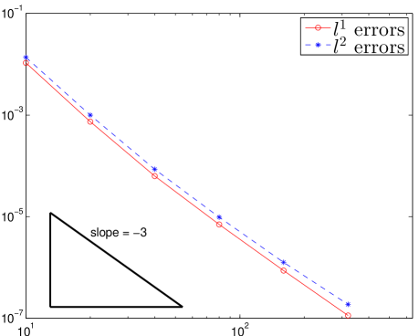
Refer to caption
(a) Errors in v2subscript𝑣2v_{2} for 1D smooth problem
Refer to caption
(b) Errors in ρ𝜌\rho for 2D smooth problem
Figure 4.1. Example 4.1: Numerical l1superscript𝑙1l^{1}- and l2superscript𝑙2l^{2}-errors at t=1𝑡1t=1. The horizontal axis represents the value of N𝑁N.

To verify the capability of DG methods with PCP limiter in resolving 1D and 2D ultra-relativistic wave configurations, three 1D Riemann problems, a 2D rotor problem, a 2D shock and cloud interaction problem, and several 2D blast problems will be solved. For those problems, before using the PCP limiting procedure, the WENO limiter [36, 47] will be implemented with the aid of the local characteristic decomposition [2] to enhance the numerical stability of high-order DG methods in resolving the strong discontinuities as well as their interactions. Different from [47], the improved WENO proposed in [8] and the “trouble” cell indicator in [26] are used here.

Example 4.2 (1D Riemann problems).

This example verifies the robustness and effectiveness of the PCP DG method by simulating three 1D Riemann problems (RP), whose initial data comprise two different constant states separated by the initial discontinuity at x=0𝑥0x=0, see Table 4.1. The computational domain is [0.5,0.5]0.50.5[-0.5,0.5] and divided into 100010001000 uniform cells.

Table 4.1. Initial data of the three 1D RPs in Example 4.2.
ρ𝜌\quad\rho\quad v1subscript𝑣1\quad v_{1}\quad v2subscript𝑣2\quad v_{2}\quad v3subscript𝑣3\quad v_{3}\quad B1subscript𝐵1\quad B_{1}\quad B2subscript𝐵2\quad B_{2}\quad B3subscript𝐵3\quad B_{3}\quad p𝑝\quad p\quad
RP I left state 1 0 0 0 5 26 26 30
right state 1 0 0 0 5 0.7 0.7 1
RP II left state 1 0 0 0 10 7 7 104superscript10410^{4}
right state 1 0 0 0 10 0.7 0.7 108superscript10810^{-8}
RP III left state 1 0.99999 0 0 100 70 70 0.10.10.1
right state 1 -0.99999 0 0 100 -70 -70 0.10.10.1
Refer to caption
Refer to caption
Refer to caption
Refer to caption
Figure 4.2. RP I in Example 4.2: The density ρ𝜌\rho (top left), velocity v1subscript𝑣1v_{1} (top right), magnetic-field B2subscript𝐵2B_{2} (bottom left), and pressure p𝑝p (bottom right) at t=0.4𝑡0.4t=0.4 obtained by the PCP DG method. The solid lines denote the reference solutions.
Refer to caption
Refer to caption
Refer to caption
Refer to caption
Figure 4.3. Same as Fig. 4.2 except for RP II.

The first two Riemann problems are similar to but more ultra than those 1D blast wave problems in [3, 19]. Specifically, the stronger magnetic field (|𝑩|37.108𝑩37.108|\mbox{\boldmath\small$B$}|\approx 37.108) appears in the left state of the first problem, while a very strong initial jump in pressure (Δp:=|pRpL|/pR1012assignΔ𝑝subscript𝑝𝑅subscript𝑝𝐿subscript𝑝𝑅superscript1012\Delta p:=|p_{R}-p_{L}|/p_{R}\approx 10^{12}) and extremely low gas pressure (the minimum plasma-beta β:=p/pm1.98×1010assign𝛽𝑝subscript𝑝𝑚1.98superscript1010\beta:=p/p_{m}\approx 1.98\times 10^{-10}) in the second problem. The numerical results of those problem at t=0.4𝑡0.4t=0.4 obtained by using the 2superscript2{\mathbb{P}}^{2}-based PCP DG method are displayed by symbols “\circ” in Figs. 4.2 and 4.3 respectively, where and hereafter the solid lines denote the reference solutions obtained by a second-order MUSCL scheme with PCP limiter over the uniform mesh of 200002000020000 cells. It is seen that the PCP DG method exhibits good resolution and strong robustness, and the results agree well with the reference ones. Without employing the PCP limiting procedure, the high-order accurate DG methods will break down quickly within few time steps due to nonphysical numerical solutions.
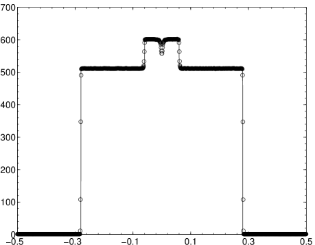
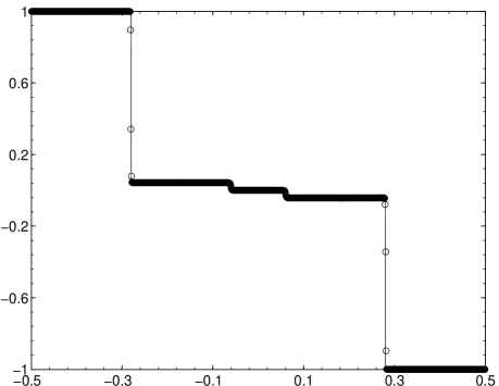
Refer to caption
Refer to caption
Refer to caption
Refer to caption
Figure 4.4. Same as Fig. 4.2 except for RP III.

The third Riemann problem describes the strong collision between two high-speed RMHD flows with a Lorentz factor of about 223.61. As a result, it is a very strongly relativistic test problem. Fig. 4.4 gives the numerical results at t=0.4𝑡0.4t=0.4 obtained by using the 2superscript2{\mathbb{P}}^{2}-based PCP DG method. As the time increases, we see that two fast and two slow reflected shock waves are produced, and a very high pressure region appears between the two slow shock waves. Those shock waves are well resolved robustly, even though there exists the well-known wall-heating type phenomenon around x=0𝑥0x=0, which is often observed in the literatures e.g. [3, 21]. It is worth mentioning that the 2superscript2{\mathbb{P}}^{2}-based DG method fails in the first time step if the PCP limiting procedure is not employed.

Example 4.3 (Rotor problem).

This is a benchmark test problem [14] extended from the classical MHD rotor problem and has been widely simulated in the literatures. It is set up on a unit domain [0.5,0.5]2superscript0.50.52[-0.5,0.5]^{2} with outflow boundary conditions. Initially, the gas pressure and magnetic field are uniform; there is a high-density disk centered at coordinate origin with radius of 0.1, rotating in anti-clockwise direction at a speed close to c𝑐c; the ambient fluid is homogeneous for r>0.115𝑟0.115r>0.115, and the fluid density and velocity are linearly with respect to r[0.1,0.115]𝑟0.10.115r\in[0.1,0.115], where r=x2+y2𝑟superscript𝑥2superscript𝑦2r=\sqrt{x^{2}+y^{2}}. Specifically, the initial data are

𝑽(x,y,0)={(10,αy,αx,0,1,0,0,1),r<0.1,(1+9δ,αyδ/r,αxδ/r,0,1,0,0,1),0.1r0.115,(1,0,0,0,1,0,0,1),r>0.115,𝑽𝑥𝑦0casessuperscript10𝛼𝑦𝛼𝑥01001top𝑟0.1superscript19𝛿𝛼𝑦𝛿𝑟𝛼𝑥𝛿𝑟01001top0.1𝑟0.115superscript10001001top𝑟0.115\mbox{\boldmath\small$V$}(x,y,0)=\begin{cases}\big{(}10,-\alpha y,\alpha x,0,1,0,0,1\big{)}^{\top},&r<0.1,\\ \big{(}1+9\delta,-\alpha y\delta/r,\alpha x\delta/r,0,1,0,0,1\big{)}^{\top},\quad&0.1\leq r\leq 0.115,\\ \big{(}1,0,0,0,1,0,0,1\big{)}^{\top},&r>0.115,\end{cases}

with δ:=(0.115r)/0.015assign𝛿0.115𝑟0.015\delta:=(0.115-r)/0.015.

Refer to caption
Refer to caption
Figure 4.5. Example 4.3: the contour plot of rest-mass density (left), and the schlieren image of Lorentz factor with magnetic lines (right) at t=0.4𝑡0.4t=0.4.

The parameter α𝛼\alpha is first taken as 9.95, which corresponds to a maximal initial Lorentz factor of about 10.01. Fig. 4.5 shows the contour plot of rest-mass density and the schlieren image of Lorentz factor at t=0.4𝑡0.4t=0.4 obtained by using the 2superscript2{\mathbb{P}}^{2}-based DG method with the PCP limiter over the uniform mesh of 400×400400400400\times 400 cells. The results agree well with those in the works [21, 47]. As one can see that winding magnetic field lines are formed and decelerates the disk speed. The central magnetic field lines are rotated almost 90superscript9090^{\circ} at t=0.4𝑡0.4t=0.4. The initial high density at the center is swept away completely and a oblong-shaped shell is formed. Our PCP method can work successfully for more ultra cases with larger α=9.99𝛼9.99\alpha=9.99 and 9.9999.9999.999 (corresponding maximal initial Lorentz factors are of about 22.37 and 70.71). However, if the PCP limiting procedure is not employed, the high-order accurate DG code breaks down.

Example 4.4 (Shock and cloud interaction problem).

This problem describes the disruption of a high density cloud by a strong shock wave. The setup is the same as that in [21]. Different from the setup in [31], the magnetic field is not orthogonal to the slab plane so that the magnetic divergence-free treatment has to be imposed. The computational domain is [0.2,1.2]×[0,1]0.21.201[-0.2,1.2]\times[0,1], with the left boundary specified as inflow condition and the others as outflow conditions. Initially, a shock wave moves to the right from x=0.05𝑥0.05x=0.05, with the left and right states 𝑽L=(3.86859,0.68,0,0,0,0.84981,0.84981,1.25115)subscript𝑽𝐿superscript3.868590.680000.849810.849811.25115top{\mbox{\boldmath\small$V$}}_{L}=(3.86859,0.68,0,0,0,0.84981,-0.84981,1.25115)^{\top} and 𝑽R=(1,0,0,0,0,0.16106,0.16106,0.05)subscript𝑽𝑅superscript100000.161060.161060.05top{\mbox{\boldmath\small$V$}}_{R}=(1,0,0,0,0,0.16106,0.16106,0.05)^{\top}, respectively. There exists a rest circular cloud centred at the point (0.25,0.5)0.250.5(0.25,0.5) with radius 0.15. The cloud has the same states to the surrounding fluid except for a higher density 30.
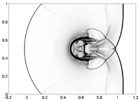
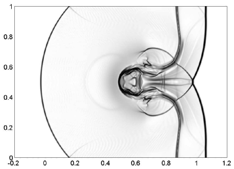
Refer to caption
Refer to caption
Figure 4.6. Example 4.4: the schlieren images of rest-mass density logarithm (left) and magnetic pressure logarithm (right) at t=1.2𝑡1.2t=1.2.

Fig. 4.6 displays the schlieren images of rest-mass density logarithm lnρ𝜌\ln\rho and magnetic pressure logarithm lnpmsubscript𝑝𝑚\ln p_{m} at t=1.2𝑡1.2t=1.2 obtained by using the 2superscript2{\mathbb{P}}^{2}-based DG method with the PCP limiter over the uniform mesh of 560×400560400560\times 400 cells. One can see that the discontinuities are captured with high resolution, and the results agree well with those in [21]. In this test, it is also necessary to use the PCP limiting procedure for the successful performance of high-order accurate DG methods. The 2superscript2{\mathbb{P}}^{2}-based DG method without the PCP limiter will fail at t0.05𝑡0.05t\approx 0.05 due to inadmissible numerical solutions.

Example 4.5 (Blast problems).

Blast problem has become a standard test for 2D RMHD numerical schemes. If the low gas pressure, strong magnetic field or low plasma-beta β:=p/pmassign𝛽𝑝subscript𝑝𝑚\beta:=p/p_{m} is involved, then simulating those ultra RMHD blast problems becomes very challenging [30]. Several different setups have been used in the literature, see e.g. [27, 31, 15, 43, 30]. Our setups are similar to that in [31, 15, 7, 43]. Initially, the computational domain [6,6]2superscript662[-6,6]^{2} is filled with a homogeneous gas at rest with adiabatic index Γ=43Γ43\Gamma=\frac{4}{3}. The explosion zone (r<0.8𝑟0.8r<0.8) has a density of 102superscript10210^{-2} and a pressure of 111, while the ambient medium (r>1𝑟1r>1) has a density of 104superscript10410^{-4} and a pressure of pa=5×10⁴subscript𝑝𝑎5superscript104p_{a}=5\times 10^{-4}, where r=x2+y2𝑟superscript𝑥2superscript𝑦2r=\sqrt{x^{2}+y^{2}}. A linear taper is applied to the density and pressure for r[0.8,1]𝑟0.81r\in[0.8,1]. The magnetic field is initialized in the x𝑥x-direction as Basubscript𝐵𝑎B_{a}. As Basubscript𝐵𝑎B_{a} is set larger, the initial ambient magnetization becomes higher (βa:=pa/pmassignsubscript𝛽𝑎subscript𝑝𝑎subscript𝑝𝑚\beta_{a}:=p_{a}/p_{m} becomes lower) and this test becomes more challenging. In the literature [31, 15, 7], Basubscript𝐵𝑎B_{a} is usually specified as 0.1, which corresponds to a moderate magnetized case (βa=0.1subscript𝛽𝑎0.1\beta_{a}=0.1). A more strongly magnetized case with Ba=0.5subscript𝐵𝑎0.5B_{a}=0.5 is tested in [43], corresponding to a lower plasma-beta βa=4×10³subscript𝛽𝑎4superscript103\beta_{a}=4\times 10^{-3}. Most existing methods in literature need some artificial treatments for the strongly magnetized case, see e.g. [27, 31]. It is reported in [15] that the RMHD code ECHO is not able to run this test with Ba>0.1subscript𝐵𝑎0.1B_{a}>0.1 if no ad hoc numerical strategy is introduced.
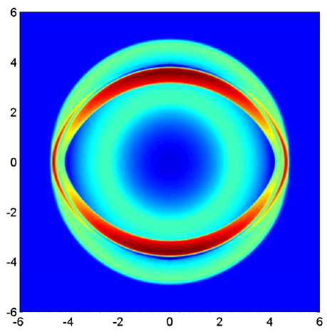
Refer to caption
Refer to caption
Refer to caption
Refer to caption
Figure 4.7. Example 4.5 with Ba=0.1subscript𝐵𝑎0.1B_{a}=0.1: the schlieren images of rest-mass density logarithm (top-left), gas pressure (top-right), Lorentz factor (bottom-left) and magnetic field strength (bottom-right) at t=4𝑡4t=4.
Refer to caption
Refer to caption
Refer to caption
Refer to caption
Figure 4.8. Same as Fig. 4.7 except for Ba=0.5subscript𝐵𝑎0.5B_{a}=0.5.
Refer to caption
Refer to caption
Refer to caption
Refer to caption
Figure 4.9. Same as Fig. 4.7 except for Ba=20subscript𝐵𝑎20B_{a}=20.

Our numerical results of this test at t=4𝑡4t=4 are shown in Fig. 4.7 for the moderately magnetized case with Ba=0.1subscript𝐵𝑎0.1B_{a}=0.1, in Fig. 4.8 for the relatively strongly magnetized case with Ba=0.5subscript𝐵𝑎0.5B_{a}=0.5, and in Fig. 4.9 for the strongly magnetized case with Ba=20subscript𝐵𝑎20B_{a}=20 (corresponding βa=2.5×10⁶subscript𝛽𝑎2.5superscript106\beta_{a}=2.5\times 10^{-6}). All of them are obtained by using the 2superscript2{\mathbb{P}}^{2}-based DG method with the PCP limiter over the uniform mesh of 400×400400400400\times 400 cells. During those simulations, the present method exhibits very good robustness without any artificial treatment. For the first two cases, our results agree quite well with those reported in [43, 7]. From Fig. 4.7, it is observed that the wave pattern of the configuration is composed by two main waves, an external fast and a reverse shock waves. The former is almost circular, while the latter is somewhat elliptic. The magnetic field is essentially confined between them, while the inner region is almost devoid of magnetization. In the case of Ba=0.5subscript𝐵𝑎0.5B_{a}=0.5, the external circular fast shock is clearly visible in the rest-mass density and in the magnetic field, but very weak. When Basubscript𝐵𝑎B_{a} is increased to 20, the external circular fast shock becomes much weaker and is only visible in the magnetic field in Fig. 4.9. As the magnetization is increased, the blast wave is confined to propagate along the magnetic field lines, creating a structure elongated in the x𝑥x-direction.

Refer to caption
Figure 4.10. Example 4.5 with Ba=100subscript𝐵𝑎100B_{a}=100: close-up of the schlieren image of |divijout𝑩|superscriptsubscriptdiv𝑖𝑗out𝑩\left|\mbox{\rm div}_{ij}^{\mbox{\tiny\rm out}}{\mbox{\boldmath\small$B$}}\right| at t=0.783𝑡0.783t=0.783 on the uniform mesh of 400×400400400400\times 400 cells.

To investigate the importance of discrete divergence-free condition (3.21) in Theorem 3.5, we now try to test a much lower plasma-beta case βa=107subscript𝛽𝑎superscript107\beta_{a}=10^{-7} (i.e. Ba=100subscript𝐵𝑎100B_{a}=100) on the mesh of 400×400400400400\times 400 cells. For such extreme case, our method breaks down at t0.783𝑡0.783t\approx 0.783. This failure results from the computed inadmissible cell averages of conservative variables, detected in the three cells centered at points (0.225,1.095)0.2251.095(-0.225,1.095), (0.165,1.095)0.1651.095(-0.165,1.095) and (0.165,1.095)0.1651.095(-0.165,-1.095), respectively. Fig. 4.10 displays the schlieren image of |divijout𝑩|superscriptsubscriptdiv𝑖𝑗out𝑩\left|\mbox{\rm div}_{ij}^{\mbox{\tiny\rm out}}{\mbox{\boldmath\small$B$}}\right| at the moment of failure. It clearly shows the subregions with large values of |divijout𝑩|superscriptsubscriptdiv𝑖𝑗out𝑩\left|\mbox{\rm div}_{ij}^{\mbox{\tiny\rm out}}{\mbox{\boldmath\small$B$}}\right|, where the condition (3.21) is violated most seriously, and the three detected cells are exactly located in those subregions. This further demonstrates that the condition (3.21) is really crucial in achieving completely PCP schemes in 2D. As mentioned in Remark 3.4, for the purpose of numerical simulation, it is possible to weaken the impact of violating (3.21) by refining the mesh. By numerical experiments, we find that our method can work successfully on a refined mesh of 600×600600600600\times 600 cells for the case of Ba=100subscript𝐵𝑎100B_{a}=100 and a extremely strongly magnetized case with Ba=1500subscript𝐵𝑎1500B_{a}=1500 (βa4.444×1010subscript𝛽𝑎4.444superscript1010\beta_{a}\approx 4.444\times 10^{-10}). The flow structures in those two cases are similar to the case of Ba=20subscript𝐵𝑎20B_{a}=20 and omitted here. To our best knowledge, the 2D blast test with so low plasma-beta is rarely considered in the literature.

5. Conclusions

The paper studied mathematical properties of the admissible state set 𝒢𝒢\mathcal{G} defined in (1.3) of the relativistic magnetohydrodynamical (RMHD) equations (1.1). In comparison with the non-relativistic and relativistic hydrodynamical cases (with the zero magnetic field), the difficulties mainly came from the extremely strong nonlinearities, no explicit formulas of the primitive variables and the flux vectors with respect to the conservative variables, and the solenoidal magnetic field. To overcome those difficulties, the first equivalent form of 𝒢𝒢\mathcal{G} with explicit constraints on the conservative vector was first skillfully discovered with the aid of polynomial root properties, and followed by the scaling invariance. The convexity of 𝒢𝒢\mathcal{G} was proved by utilizing the semi-positive definiteness of the second fundamental form of a hypersurface, and then the second equivalent form of 𝒢𝒢\mathcal{G} and the orthogonal invariance were obtained. It was verified that the Lax-Friedrichs (LxF) splitting property did not hold in general when the magnetic field was nonzero. However, by combining the convex combination of some LxF splitting terms with a “discrete divergence-free” condition for the magnetic field, the generalized LxF splitting properties were subtly discovered with a constructive inequality and some pivotal techniques. This revealed in theory for the first time the close connection between the “discrete divergence-free” condition and the physical-constraints-preserving (PCP) property of numerical schemes.

The above mathematical properties were footstone of studying PCP numerical schemes for RMHDs. Based on the resulting theoretical results, several 1D and 2D PCP schemes were studied for the first time. In the 1D case, a first-order accurate LxF type scheme was first proved to be PCP under the CFL condition. Then, the high-order accurate 1D PCP schemes were proposed via a PCP limiter, which was designed by using the first equivalent form of 𝒢𝒢\mathcal{G}. In the 2D case, the “discrete divergence-free” condition and PCP property were analyzed for a first-order accurate LxF type scheme, and followed by two sufficient conditions for high-order accurate PCP schemes. Several numerical experiments were conducted to demonstrate the theoretical analyses and the performance of numerical schemes as well as the importance of discrete divergence-free condition in achieving genuinely PCP scheme in 2D. The studies on the PCP schemes may be easily extended to the three-dimensional case by Theorem 2.6, the non-uniform or unstructured meshes by Theorem 2.7, and the general EOS case by the similar discussions in [40].

Acknowledgements

This work was partially supported by the National Natural Science Foundation of China (Nos. 91330205 & 11421101).

References

  • [1] M. Anderson, E.W. Hirschmann, S.L. Liebling and D. Neilsen, Relativistic MHD with adaptive mesh refinement, Class. Quantum Grav. 23 (2006) 6503–6524.
  • [2] L. Antón, J.A. Miralles, J.M. Martí, J.M. Ibáñez, M.A. Aloy and P. Mimica, Relativistic magnetohydrodynamics: renormalized eigenvectors and full wave decomposition Riemann solver, Astrophys. J. Suppl. Ser. 188 (2010) 1–31.
  • [3] D.S. Balsara, Total variation diminishing scheme for relativistic magnetohydrodynamics, Astrophys. J. Suppl. Ser. 132 (2001) 83–101.
  • [4] D.S. Balsara, Second-order-accurate schemes for magnetohydrodynamics with divergence-free reconstruction, Astrophys. J. Suppl. Ser. 151 (2004) 149–184.
  • [5] D.S. Balsara, Divergence-free reconstruction of magnetic fields and WENO schemes for magnetohydrodynamics, J. Comput. Phys. 228 (2009) 5040–5056.
  • [6] D.S. Balsara, Self-adjusting, positivity preserving high order schemes for hydrodynamics and magnetohydrodynamics, J. Comput. Phys. 231 (2012) 7504–7517.
  • [7] D.S. Balsara and J. Kim, A subluminal relativistic magnetohydrodynamics scheme with ADER-WENO predictor and multidimensional Riemann solver-based corrector, J. Comput. Phys. 312 (2016) 357–384.
  • [8] R. Borges, M. Carmona, B. Costa and W. S. Don, An improved weighted essentially nonoscillatory scheme for hyperbolic conservation laws, J. Comput. Phys. 227 (2008) 3101–3211.
  • [9] J.U. Brackbill and D.C. Barnes, The effect of nonzero 𝑩𝑩\nabla\cdot\mbox{\boldmath\small$B$} on the numerical solution of the magnetodyndrodynamic equations, J. Comput. Phys. 35 (1980) 426–430.
  • [10] Y. Cheng, F.Y. Li, J.X. Qiu and L.W. Xu, Positivity-preserving DG and central DG methods for ideal MHD equations, J. Comput. Phys. 238 (2013) 255–280.
  • [11] A. J. Christlieb, Y. Liu, Q. Tang and Z.F. Xu, Positivity-preserving finite difference weighted ENO schemes with constrained transport for ideal magnetohydrodynamic equations, SIAM J. Sci. Comput. 37 (2015) A1825–A1845.
  • [12] B. Cockburn, S.C. Hu and C.-W. Shu, The Runge-Kutta local projection discontinuous Galerkin finite element method for conservation laws IV: the multidimensional case, Math. Comp. 54 (1990) 545–581.
  • [13] M. Cissoko, Detonation waves in relativistic hydrotlynamics, Phys. Rev. D 45 (1992) 1045–1052.
  • [14] L. Del Zanna, N. Bucciantini and P. Londrillo, An efficient shock-capturing central-type scheme for multidimensional relativistic flows II. Magnetohydrodynamics, Astron. Astrophys. 400 (2003) 397–413.
  • [15] L. Del Zanna, O. Zanotti, N. Bucciantini and P. Londrillo, ECHO: a Eulerian conservative high-order scheme for general relativistic magnetohydrodynamics and magnetodynamics, Astron. Astrophys. 473 (2007) 11–30.
  • [16] C.R. Evans and J.F. Hawley, Simulation of magnetodydrodynamic flows: A constrained transport method, Astrophys. J. 332 (1988) 659–677.
  • [17] J.A. Font, Numerical hydrodynamics and magnetohydrodynamics in general relativity, Living Rev. Relativity 11 (2008) 7.
  • [18] K.O. Friedrichs, On the laws of relativistic electro-magneto-fluid dynamics, Comm. Pure Appl. Math. 27 (1974) 749–808.
  • [19] B. Giacomazzo and L. Rezzolla, The exact solution of the Riemann problem in relativistic magnetohydrodynamics, J. Fluid Mech. 562 (2006) 223–259.
  • [20] S. Gottlieb, D.J. Ketcheson and C.-W. Shu, High order strong stability preserving time discretizations, J. Sci. Comput. 38 (2009) 251–289.
  • [21] P. He and H.Z. Tang, An adaptive moving mesh method for two-dimensional relativistic magnetohydrodynamics, Computers & Fluids 60 (2012) 1–20.
  • [22] V. Honkkila and P. Janhunen, HLLC solver for ideal relativistic MHD, J. Comput. Phys. 223 (2007) 643–656.
  • [23] B. van der Holst, R. Keppens, and Z. Meliani, A multidimensional grid-adaptive relativistic magnetofluid code, Comput. Phys. Comm. 179 (2008) 617–627.
  • [24] L.D. Jonker, Immersions with semi-definite second fundamental forms, Canad. J. Math. 27 (1975) 610–617.
  • [25] J. Kim and D.S. Balsara, A stable HLLC Riemann solver for relativistic magnetohydrodynamics, J. Comput. Phys. 270 (2014) 634–639.
  • [26] L. Krivodonova, J. Xin, J.-F. Remacle, N. Chevaugeon and J.E. Flaherty, Shock detection and limiting with discontinuous Galerkin methods for hyperbolic conservation laws, Appl. Numer. Math. 48 (2004) 323–338.
  • [27] S.S. Komissarov, A Godunov-type scheme for relativistic magnetohydrodynamics, Mon. Not. R. Astron. Soc. 303 (1999) 343–366.
  • [28] F.Y. Li and C.-W. Shu, Locally divergence-free discontinuous Galerkin methods for MHD equations, J. Sci. Comput. 22 (2005) 413–442.
  • [29] F.Y. Li, L.W. Xu and S. Yakovlev, Central discontinuous Galerkin methods for ideal MHD equations with the exactly divergence-free magnetic field, J. Comput. Phys. 230 (2011) 4828–4847.
  • [30] J.M. Martí and E. Müller, Grid-based methods in relativistic hydrodynamics and magnetohydrodynamics, Living Rev. Comput. Astrophys. 1 (2015) 3.
  • [31] A. Mignone and G. Bodo, An HLLC Riemann solver for relativistic flows–II. Magnetohydrodynamics, Mon. Not. R. Astron. Soc. 368 (2006) 1040–1054.
  • [32] T. Miyoshi and K. Kusano, A multi-state HLL approximate Riemann solver for ideal magnetohydrodynamics, J. Comput. Phys. 208 (2005) 315–344.
  • [33] W.I. Newman and N. D. Hamlin, Primitive variable determination in conservative relativistic magnetohydrodynamic simulations, SIAM J. Sci. Comput. 36 (2014) B661–B683.
  • [34] S.C. Noble, C.F. Gammie, J.C. McKinney and L.D. Zanna, Primitive variable solvers for conservative general relativistic magnetohydrodynamics, Astrophys. J., Suppl. Ser. 641 (2006) 626–637.
  • [35] S. Qamar and G. Warnecke, A high-order kinetic flux-splitting method for the relativistic magnetohydrodynamics, J. Comput. Phys. 205 (2005) 182–204.
  • [36] J. Qiu and C.-W. Shu, Runge-Kutta discontinuous Galerkin method using WENO limiters, SIAM J. Sci. Comput. 26 (2005) 907–929.
  • [37] J.A. Rossmanith, An unstaggered, high-resolution constrained transport method for magnetohydrodynamic flows, SIAM J. Sci. Comput. 28 (2006) 1766–1797.
  • [38] G. Tóth, The 𝑩=0𝑩0\nabla\cdot\mbox{\boldmath\small$B$}=0 constraint in shock-capturing magnetohydrodynamics codes, J. Comput. Phys. 161 (2000) 605–652.
  • [39] K.L. Wu and H.Z. Tang, High-order accurate physical-constraints-preserving finite difference WENO schemes for special relativistic hydrodynamics, J. Comput. Phys. 298 (2015) 539–564.
  • [40] K.L. Wu and H.Z. Tang, Physical-constraints-preserving central discontinuous Galerkin methods for special relativistic hydrodynamics with a general equation of state, accepted by Astrophys. J. Suppl. Ser., 2016.
  • [41] Y. Xing, X. Zhang and C.-W. Shu, Positivity-preserving high order well-balanced discontinuous Galerkin methods for the shallow water equations, Adv. Water Res. 33 (2010) 1476–1493.
  • [42] H. Yang and F.Y. Li, Stability analysis and error estimates of an exactly divergence-free method for the magnetic induction equations, ESAIM: Math. Model. Numer. Anal. 50 (2016) 965–993.
  • [43] O. Zanotti, F. Fambri and M. Dumbser, Solving the relativistic magnetohydrodynamics equations with ADER discontinuous Galerkin methods, a posteriori subcell limiting and adaptive mesh refinement, Mon. Not. R. Astron. Soc. 452 (2015) 3010–3029.
  • [44] X. Zhang and C.-W. Shu, On maximum-principle-satisfying high order schemes for scalar conservation laws, J. Comput. Phys. 229 (2010) 3091–3120.
  • [45] X. Zhang and C.-W. Shu, On positivity-preserving high-order discontinuous Galerkin schemes for compressible Euler equations on rectangular meshes, J. Comput. Phys. 229 (2010) 8918–8934.
  • [46] X.X. Zhang and C.-W. Shu, Maximum-principle-satisfying and positivity-preserving high-order schemes for conservation laws: survey and new developments, Proc. R. Soc. A 467 (2011) 2752–2776.
  • [47] J. Zhao and H.Z. Tang, Runge-Kutta discontinuous Galerkin methods for the special relativistic magnetohydrodynamics, arXiv:1610.03404, 2016.