Observational biases for transiting planets

Abstract

Observational biases distort our view of nature, such that the patterns we see within a surveyed population of interest are often unrepresentative of the truth we seek. Transiting planets currently represent the most informative data set on the ensemble properties of exoplanets within 1 au of their star. However, the transit method is inherently biased due to both geometric and detection-driven effects. In this work, we derive the overall observational biases affecting the most basic transit parameters from first principles. By assuming a trapezoidal transit and using conditional probability, we infer the expected distribution of these terms both as a joint distribution and in a marginalized form. These general analytic results provide a baseline against which to compare trends predicted by mission-tailored injection/recovery simulations and offer a simple way to correct for observational bias. Our results explain why the observed population of transiting planets displays a non-uniform impact parameter distribution, with a bias towards near-equatorial geometries. We also find that the geometric bias towards observed planets transiting near periastron is attenuated by the longer durations which occur near apoastron. Finally, we predict that the observational bias with respect to ratio-of-radii is super-quadratic, scaling as $(R_{P}/R_{\star})^{5/2}$, driven by an enhanced geometric transit probability and modestly longer durations.

1 Introduction

The occurrence rate and properties of extrasolar planetary systems has been an active area of astronomical research in recent years. These topics pertain to our uniqueness in the cosmos and affect the technical requirements of future instrumentation (e.g. see Dalcanton et al. 2015).

The primary Kepler Mission, which was designed to be a statistical mission, has provided a wealth of data to address these questions. By detecting the decrement in stellar brightness caused by planets passing in front of their stars, Kepler has uncovered more than 4000 planetary candidates to date (Burke et al., 2015). However, the transit method, whilst evidently highly successful, is also plagued with several severe and well-known observational biases. Specifically, two dominant forms of bias obscure our view of the true exoplanet population: a geometric bias and a detection bias. For example, the former leads to a bias towards detecting short-period planets (Beatty & Gaudi, 2008) and the latter leads to a bias towards larger planets.

Correcting for these biases is crucial when interpreting the Kepler data to make inferences about the underlying population. The most assured approach for correcting for these biases is a full end-to-end numerical simulation of the detection efficiency (e.g. see Petigura et al. 2013; Christiansen et al. 2015; Dressing & Charbonneau 2015). In such a simulation, one generates a population of fake planets, creates corresponding fake time series with transits, and pushes the fake time series through the detection pipeline of interest to numerically compute the detection efficiency as a function of the input parameters.

These numerical approaches are tailored to the specific mission of interest and may be sensitive to the assumed population of injected planets. Nevertheless, this method is undoubtedly the most robust way to perform bias corrections on complex data sets like Kepler. Despite this, we argue that there is also great value in considering the problem of bias correction analytically. Analytic investigations can provide a deeper understanding of the underlying problem than possible through Monte Carlo simulations, which can often obscure the explanations of observed patterns. Moreover, analytic results can be interpreted in any context, rather than being tailored to a specific mission. This approach therefore complements the numerical work, offering insights into which trends are instrument-specific and which are inherent to transit surveys.

Several previous works have investigated some of the biases affecting transit surveys analytically. For example, Barnes (2007) showed that the geometric bias of transits favors the detection of eccentric transiting planets. Burke (2008) extended upon these ideas and showed how the transit duration is also affected by orbital eccentricity, leading to an overall decrease in the detectability of eccentric planets. Beatty & Gaudi (2008) consider the overall detection yield from a transit survey in an analytic framework, revealing the dependence on orbital period.

In these previous works, the transit light curves were assumed to be well-approximated by a simple box-like shape. Whilst a reasonable first approximation, this assumption prohibits the investigation of V-shaped grazing transits and is, as we show later, an assumption which could be relaxed without abandoning an analytic framework. Additionally, previous works tend to focus on the expected detection yields from transit surveys (e.g. Beatty & Gaudi 2008; Burke 2008), as opposed to how the observed population parameters are modified by the various biases. In Kipping (2014), we used conditional probability to explore the distortion to the eccentricity distribution, but that work was limited to just geometric bias (i.e., no detection bias) and also only considered eccentricity and argument of periastron.

In this paper, we aim to build upon the aforementioned works to derive the effect of both geometric and detection bias on the basic parameters observable with transits. By using a trapezoidal transit model, we also investigate the limit of grazing transits and use our model to explain previously observed trends from the Kepler transit survey.

The paper is organized as follows. In §2, we derive an analytic expression for the SNR of a trapezoidal transit, including grazing geometries. In §3, we show how making some approximations to this result allows us to write down a simple form for the joint distribution of the transit parameters. We build upon this work in §4, deriving a more accurate set of expressions for the joint and marginalized distributions that result and extending the formalism to include occultations. Finally, we summarize our findings in §5.

2 Signal-to-Noise Ratio of a Transit

2.1 SNR of a trapezoidal transit

In order to analytically model detection bias, we begin by deriving the SNR of the transit light curve as a function of the basic transit parameters.

A transit is a decrease in the apparent brightness, or more specifically the received intensity, $I(t)$, of a star as a function of time, $t$. The received intensity may be defined as the number of photons received per unit time. Away from transit events (‘out-of-transit’), then, a ‘vanilla’ star displaying no changes in brightness would cause our detector to receive an intensity

$$I_{\mathrm{out}}(t) =\Gamma,$$ (1)

where $\Gamma$ represents the nominal photon collection rate. In order to actually measure the photon collection rate, we have to collect photons over a specific time interval ($t_{i}\to t_{f}$) and then divide by said interval. This is equivalent to calculating the mean of the function $I(t)$ via

$$\overline{I}= \frac{\int_{t=t_{i}}^{t_{f}}I(t)\mathrm{d}t}{\int_{t=t_{i}}^{t_{f}}\mathrm{d}t}.$$ (2)

In the out-of-transit case, the above yields the simple result $\overline{I_{\mathrm{out}}}=\Gamma$.

In the case of a star accompanied by a transiting planet, the intensity will be periodically attenuated by the eclipse of the planet. Following Carter et al. (2008), we approximate the shape of the transit light curve as a trapezoid in what follows. As was shown in fig. 1 of Carter et al. (2008), four key times, $t_{1}<t_{2}<t_{3}<t_{4}$, as well as a depth, $\delta$, define the shape of the transit:

$$I_{\mathrm{in}}(t)=\Gamma\left\{\begin{array}[]{ll}1-\delta&t_{2}\leq t\leq t_{3}\\ 1-\frac{\delta(t-t_{1})}{t_{2}-t_{1}}&t_{1}<t<t_{2}\\ 1-\frac{\delta(t_{4}-t)}{t_{4}-t_{3}}&t_{3}<t<t_{4}\end{array}\right..$$ (3)

The fractional change in the measured intensity defines the ‘signal’ in the case of transits. We express the signal as

$$S= \frac{\overline{I_{\mathrm{out}}}-\overline{I_{\mathrm{in}}}}{\overline{I_{\mathrm{out}}}},$$ (4)

where the subscripts ‘in’ and ‘out’ denote in- and out-of-transit. Evaluating $\overline{I_{\mathrm{in}}}$ using Equations (2) and (3), then substituting into Equation (4) and replacing $(t_{4}-t_{1})$ and $(t_{3}-t_{2})$ with $T_{14}$ and $T_{23}$, respectively, yields

$$S= \Big{(}\frac{T_{14}+T_{23}}{2T_{14}}\Big{)}\delta.$$ (5)

In the limit of a box-like transit, we have $T_{14}\to T$ and $T_{23}\to T$, which reproduces the classic result of $S=\delta$.

Having calculated the ‘signal,’ we now turn our attention to the ‘noise.’ Since $\overline{I_{\mathrm{in}}}$ and $\overline{I_{\mathrm{out}}}$ are independent of one another, the error on $S$, which we define as $\sigma_{S}$ (the ‘noise’), may be calculated via quadrature as

$$\sigma_{S}^{2}= (\partial_{\overline{I_{\mathrm{out}}}}S)^{2}\sigma_{\overline{I_{\mathrm{out}}}}^{2}+(\partial_{\overline{I_{\mathrm{in}}}}S)^{2}\sigma_{\overline{I_{\mathrm{in}}}}^{2},$$

$$\qquad= \frac{\overline{I_{\mathrm{out}}}^{2}\sigma_{\overline{I_{\mathrm{in}}}}^{2}+\overline{I_{\mathrm{in}}}^{2}\sigma_{\overline{I_{\mathrm{out}}}}^{2}}{\overline{I_{\mathrm{out}}}^{4}}.$$ (6)

Since our detector is essentially a photon counter, the uncertainty on the terms $\overline{I_{\mathrm{in}}}$ and $\overline{I_{\mathrm{out}}}$ may be calculated using Poisson statistics. Specifically, one expects the uncertainty on the mean intensity $\overline{I(t)}$ to be given by

$$\sigma_{\overline{I}} =\frac{\sqrt{\int_{t=t_{i}}^{t_{f}}I(t)\mathrm{d}t}}{\int_{t=t_{i}}^{t_{f}}\mathrm{d}t}.$$ (7)

Evaluating $\sigma_{\overline{I_{\mathrm{in}}}}$ and $\sigma_{\overline{I_{\mathrm{out}}}}$ using Equation (7) and then substituting the results into Equation (6), we find

$$\sigma_{S} =\sqrt{\frac{(T_{14}-W\delta)(T_{\mathrm{obs}}+T_{14}-W\delta)}{T_{14}^{2}T_{\mathrm{obs}}\Gamma}},$$ (8)

where $W\equiv(T_{14}+T_{23})/2$ and $T_{\mathrm{obs}}$ is the duration over which the out-of-transit intensity is observed. Finally, then, the SNR of a single trapezoidal transit is

$$\mathrm{SNR}_{\mathrm{single}} =\frac{W\delta\sqrt{T_{\mathrm{obs}}\Gamma}}{\sqrt{(T_{14}-W\delta)(T_{\mathrm{obs}}+T_{14}-W\delta)}}.$$ (9)

In most instances, the out-of-transit baseline is much longer than the in-transit observations in order to reduce the uncertainty in the transit measurement. In this limit of $T_{\mathrm{obs}}\gg T_{14}$, we have

$$\lim_{T_{\mathrm{obs}}\gg T_{14}}\mathrm{SNR}_{\mathrm{single}} =\frac{W\delta\sqrt{\Gamma}}{\sqrt{T_{14}-W\delta}}$$ (10)

In the small-planet case of $\delta\ll 1$ (appropriate even for the Jupiter-Sun system), this becomes

$$\lim_{\delta\ll 1}\lim_{T_{\mathrm{obs}}\gg T_{14}}\mathrm{SNR}_{\mathrm{single}} =\delta\sqrt{\Gamma}\frac{W}{\sqrt{T_{14}}}.$$ (11)

In what follows, $T_{\mathrm{obs}}\gg T_{14}$ and $\delta\ll 1$ are adopted as assumptions, and we do not explicitly state them in subsequent expressions.

2.2 Accounting for grazing transits

Equation (11) provides a simple and practical estimate for the SNR of a trapezoidal transit. However, it is framed in terms of the depth, $\delta$, which is not equal to $p^{2}$ (the ratio-of-radii squared) in cases where $(1-p)<b<(1+p)$, corresponding to so-called grazing transits. In such instances, $\delta<p^{2}$ and requires calculating the area of partial overlap between the planet’s disc and that of the star. This is commonly done using the $\lambda$ function, defined in Equation 1 of Mandel & Agol (2002) as

$$\lambda(p,\mathcal{S})=\frac{1}{\pi}\Bigg{(}p^{2}\kappa_{0}+\kappa_{1}-\sqrt{\frac{4\mathcal{S}^{2}-(1-\mathcal{S}^{2}-p^{2})^{2}}{4}}\Bigg{)},$$ (12)

where

$$\kappa_{0}\equiv\cos^{-1}\Big{(}\frac{p^{2}+\mathcal{S}^{2}-1}{2p\mathcal{S}}\Big{)},$$ (13)

$$\kappa_{1}\equiv\cos^{-1}\Big{(}\frac{1-p^{2}+\mathcal{S}^{2}}{2\mathcal{S}}\Big{)},$$ (14)

and $\mathcal{S}$ is the sky-projected planet–star separation in stellar radii. Accordingly, we now express

$$\delta(p,b)=\left\{\begin{array}[]{ll}p^{2}&0\leq b<1-p\\ \lambda(p,b)&1-p\leq b<1+p\\ 0&1+p\leq b<\infty\end{array}\right..$$ (15)

We may now modify the $\mathrm{SNR}_{\mathrm{single}}$ expression (Equation 11) to account for grazing events as

$$\mathrm{SNR}_{\mathrm{single}}=\left\{\begin{array}[]{ll}\Big{(}\frac{T_{14}+T_{23}}{2\sqrt{T_{14}}}\Big{)}p^{2}\sqrt{\Gamma}&0\leq b<1-p\\ \Big{(}\frac{\sqrt{T_{14}}}{2}\Big{)}\lambda(p,b)\sqrt{\Gamma}&1-p\leq b<1+p\\ 0&1+p\leq b<\infty\end{array}\right.,$$ (16)

where the grazing case is evaluated by appreciating that $T_{23}=0$ in such instances. In the limit of a box-like transit, these expressions are equivalent to Equation 19 of Carter et al. (2008).

2.3 Approximating the SNR equation

In order to understand the relationship between SNR and impact parameter, $b$, we need to rewrite Equation (16) by evaluating the various durations. To this end, we employ the “one term” transit duration function from Kipping (2010) (Equation 15 of that work) in what follows. We initially seek a simple and approximate formula, with the full SNR expression of Equation (16) serving as a useful comparison for the accuracy of proposed approximations.

We start by assuming that $p\ll 1$, the small-planet approximation, for which the first implication is that grazing transits contribute negligibly to the SNR function, and thus we need only consider trapezoidal transits. Under this approximation, it also true that one expects $W=(T_{14}+T_{23})/2\simeq\tilde{T}$, as defined in Kipping (2010), which reduces two of the duration terms to just one. We then proceed to make a small-angle approximation on the inverse sine functions ($\sin^{-1}(x)\simeq x$) within the duration terms, equivalent to assuming $a_{R}\gg 1$, which is valid for the vast majority of exoplanets. In total, then, we approximate $a_{R}\gg 1$, $W\to\tilde{T}$ and $p\ll 1$, such that

$$\lim_{a_{R}\gg 1}\lim_{W\to\tilde{T}}\lim_{p\ll 1}\mathrm{SNR}_{\mathrm{single}}=\nu_{\mathrm{single}}(1-b^{2})^{1/4}p^{2},$$ (17)

where we have defined

$$\nu_{\mathrm{single}} \equiv\Bigg{(}\frac{3}{G\pi^{2}}\Bigg{)}^{1/6}\rho_{\star}^{-1/6}P^{1/6}\Bigg{(}\frac{(1-e^{2})^{1/4}}{(1+e\sin\omega)^{1/2}}\Bigg{)}\Gamma^{1/2}.$$ (18)

The accuracy of Equation (17) versus the more accurate Equation (16) is illustrated later in Figs 2 and 3.

Whilst the above is derived for single transits, one often deals with multiple events, in which case the SNR is expected to increase with the square root of the number of events. Within a given baseline of observations, $T_{\mathrm{obs}}$, we therefore expect the SNR to increase by $\sqrt{T_{\mathrm{obs}}/P}$, since shorter-period planets fit more transits in within $T_{\mathrm{obs}}$, such that

$$\lim_{a_{R}\gg 1}\lim_{W\to\tilde{T}}\lim_{p\ll 1}\mathrm{SNR}_{\mathrm{multi}}=\nu_{\mathrm{multi}}(1-b^{2})^{1/4}p^{2},$$ (19)

where

$$\nu_{\mathrm{multi}} \equiv\Bigg{(}\frac{3}{G\pi^{2}}\Bigg{)}^{1/6}\rho_{\star}^{-1/6}P^{-1/3}\Bigg{(}\frac{(1-e^{2})^{1/4}}{(1+e\sin\omega)^{1/2}}\Bigg{)}\sqrt{\Gamma T_{\mathrm{obs}}}.$$ (20)

3 Conditional Probability Distributions

3.1 Probability of detection

In what follows, we use the symbol $\hat{d}$ to denote ‘transit detected.’ Let us group the various parameters in Equation (19) into a vector $\boldsymbol{\Theta}=\{p,b,P,\rho_{\star},e,\omega\}$. We define the probability of detecting a transit conditioned upon these transit parameters and the fact that the system geometry permits the planet to transit at all as $\mathrm{Pr}(\hat{d}|\boldsymbol{\Theta},\hat{b})$, where $\hat{b}$ is short-hand for $b<1$. In what follows, a basic assumption of this work is that

$$\mathrm{Pr}(\hat{d}|\boldsymbol{\Theta},\hat{b})\propto\mathrm{SNR}_{\mathrm{multi}},$$ (21)

which states that the probability of detecting a transit is proportional to its SNR. Whilst this statement is intuitive, it is worth pausing to consider its validity in the case of the most comprehensive transit survey to date, Kepler.

Figure 1: Probability of detecting an injected transit of a known SNR into the Kepler pipeline for FGK dwarfs (data taken from Christiansen et al. 2015). The top-left key lists various models in chronological publication order, where the last is derived here using updated parameters for the Fressin et al. (2013) ramp, which provides a reasonable description with a sufficiently analytically simple model to make progress within this work.

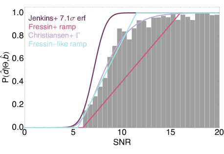
The formal criterion for a Kepler detection is that the transit events display an SNR exceeding 7.1 (Jenkins et al., 2010). This assumption implies that the probability of detection, $\mathrm{Pr}(\hat{d}|\boldsymbol{\Theta},\hat{b})$, follows a cumulative normal distribution centred on 7.1 with a standard deviation of unity (Christiansen et al., 2015), as shown in Fig. 1.

In practice, this simple model has been found to be an unrealistic representation of the Kepler detections, with Fressin et al. (2013) arguing that modelling $\mathrm{Pr}(\hat{d}|\boldsymbol{\Theta},\hat{b})$ as linearly proportional to SNR (the same assumption we make here) describes the data far better. However, recently, Christiansen et al. (2015) used injection/recovery simulations to show that $\mathrm{Pr}(\hat{d}|\boldsymbol{\Theta},\hat{b})$ is best described by a $\Gamma$ cumulative distribution, as shown in Fig. 1. Nevertheless, fitting updated parameters to the Fressin et al. (2013) ramp model conditioned on the FGK dwarf injection tests of Christiansen et al. (2015) reveals that a linear model still provides an excellent description, as evident in Fig. 1. Due to its analytic convenience, reasonable accuracy, and general applicability to other surveys, we therefore adopt the linearly proportional assumption throughout.

We also note that detection functions tend to truncate to unity probability at a high SNR, and our model does not directly account for this truncation. However, in such a regime, the transit surveys are complete, detection bias plays no role, and one may use the geometric bias terms derived in this work alone.

3.2 Joint probability distribution of the transit parameters

Using Bayes’ theorem, the joint probability distribution of $\boldsymbol{\Theta}$, conditioned upon $\hat{d}$ and $\hat{b}$, is given by

$$\mathrm{Pr}(\boldsymbol{\Theta}|\hat{d},\hat{b}) \propto\mathrm{Pr}(\hat{d}|\boldsymbol{\Theta},\hat{b})\mathrm{Pr}(\boldsymbol{\Theta}|\hat{b}),$$ (22)

We take a brief aside to explore the $\mathrm{Pr}(\boldsymbol{\Theta}|\hat{b})$ term. From Kipping (2014), Equation 2, the probability of a transit, defined as being $b<1$, modified to replace $a_{R}\to\rho_{\star}$, is given by

$$\mathrm{Pr}(\hat{b}|\boldsymbol{\Theta}) =\Bigg{(}\frac{3\pi}{G}\Bigg{)}^{1/3}P^{-2/3}\rho_{\star}^{-1/3}\Bigg{(}\frac{1+e\sin\omega}{1-e^{2}}\Bigg{)}.$$ (23)

The above essentially assumes $p\ll 1$, since grazing events do not contribute as ‘transits.’ Using Bayes’ theorem, then, one may write that

$$\mathrm{Pr}(\boldsymbol{\Theta}|\hat{b}) \propto\mathrm{Pr}(\hat{b}|\boldsymbol{\Theta})\mathrm{Pr}(\boldsymbol{\Theta}),$$ (24)

and thus

$$\mathrm{Pr}(\boldsymbol{\Theta}|\hat{d},\hat{b}) \propto\mathrm{Pr}(\hat{d}|\boldsymbol{\Theta},\hat{b})\mathrm{Pr}(\hat{b}|\boldsymbol{\Theta})\mathrm{Pr}(\boldsymbol{\Theta}).$$ (25)

where it is evident from Equation (23) that $\mathrm{Pr}(\hat{b}|\boldsymbol{\Theta})$ is in fact independent of $p$ and $b$. Since $\mathrm{Pr}(\hat{d},\hat{b}|\boldsymbol{\Theta})\propto\mathrm{Pr}(\hat{d}|\boldsymbol{\Theta},\hat{b})\mathrm{Pr}(\hat{b}|\boldsymbol{\Theta})$, we may re-write Equation (25) as

$$\underbrace{\mathrm{Pr}(\boldsymbol{\Theta}|\hat{d},\hat{b})}_{\text{overall dist.}} \propto\underbrace{\mathrm{Pr}(\hat{d},\hat{b}|\boldsymbol{\Theta})}_{\text{observational bias}}\underbrace{\mathrm{Pr}(\boldsymbol{\Theta})}_{\text{intrinsic dist.}}.$$ (26)

where $\mathrm{Pr}(\hat{d},\hat{b}|\boldsymbol{\Theta})$ is proportional to the product of Equations (19) and (23), yielding

$$\mathrm{Pr}(\hat{d},\hat{b}|\boldsymbol{\Theta}) \propto\kappa(1-b^{2})^{1/4}p^{2},$$ (27)

where we define

$$\kappa \equiv P^{-1}\rho_{\star}^{-1/2}(1+e\sin\omega)^{1/2}(1-e^{2})^{-3/4}.$$ (28)

It is worth noting that in the above, all of the terms except $e$ and $\omega$ are separable, and Equation (27) can be expressed as

$$\mathrm{Pr}(\hat{d},\hat{b}|\boldsymbol{\Theta}) \propto\mathrm{Pr}(\hat{d},\hat{b}|P)\mathrm{Pr}(\hat{d},\hat{b}|\rho_{\star})\mathrm{Pr}(\hat{d},\hat{b}|e,\omega)\mathrm{Pr}(\hat{d},\hat{b}|b)\mathrm{Pr}(\hat{d},\hat{b}|p).$$ (29)

If $\mathrm{Pr}(\boldsymbol{\Theta})$, the intrinsic distribution, is also separable, then the result above implies that $\mathrm{Pr}(\boldsymbol{\Theta}|\hat{d},\hat{b})$ is separable too. In practice, the intrinsic distribution is unlikely to be truly separable (even if assumed so for convenience). In particular, the distribution of ratio-of-radii, $p$, is likely covariant with terms such as $\rho_{\star}$. This means that inverse sampling from the overall prior will be hierarchically conditional, assuming it is even possible to write down a closed form for such a distribution. For this reason, we argue that inverse transform sampling is not a practical way of sampling the distribution.

3.3 Using the conditional probability distributions as a prior

As a brief aside, we discuss here why generally we do not recommend blindly using the derived conditional probabilities as priors in the analysis of individual transiting planets. To centre the discussion, we first consider the case of the mean stellar density, $\rho_{\star}$.

The likelihood function of a real transit fit exhibits a strong negative covariance between $\rho_{\star}$ and $b$ (Carter et al., 2008). Our derived bias terms favour a low $\rho_{\star}$ and a low $b$, i.e., they are positively covariant. Furthermore, the exponential $\rho_{\star}$ bias quickly outweighs the softer $b$ bias, and thus, when convolved with the likelihood effect, transit fits would tend to be driven towards low $\rho_{\star}$ parameter space but high, near-grazing $b$. This means the $b$ bias is essentially washed out, and the overall fit is driven towards low $\rho_{\star}$.

One reason why this is problematic is that, thanks to our knowledge of stellar evolution, we understand that low-density stars will have larger stellar radii, and therefore, the same sized planet is less likely to be detected around a low-density than a high-density star. This problem could be resolved if we actually knew the true joint (and covariant) intrinsic prior of $\rho_{\star}$ and $p$, which would correct for this effect. Of course, the intrinsic prior is generally unavailable.

Since many of the transit parameters display covariance in the likelihood function to some extent (Carter et al., 2008), particularly in the case of realistic transits with limb darkening and sparse sampling, the above effect is general. For these reasons, we do not advocate blindly using these distributions as priors in individual transit light-curve fits.

4 Extending to Grazing Transits

4.1 A more accurate SNR

Based on the analytical form for the SNR of a trapezoidal transit and the geometric bias of the transit method, we have derived the conditional probability of the basic transit parameters for a planet detected to transit, $\mathrm{Pr}(\boldsymbol{\Theta}|\hat{d},\hat{b})$.

In order to do this, we made various approximations to the SNR expression shown in Equation (16). The result of these approximations was a simple, multiplicative form of the joint distribution (Equation 27). Whilst this is undoubtedly useful, especially for illustrating overall trends, we describe here a more accurate estimate.

The biggest problem with Equation (27) is that $b=1$ has zero probability, but the SNR should not go to zero until $b=(1+p)$. Therefore, our proposed simple form truncates a part of parameter space. To derive a superior approximation, we return to Equation (16).

In the case of non-grazing events, we first tried approximating $(T_{14}+T_{23})/2\simeq\tilde{T}$ (see Kipping 2010 for definitions). However, this approximation becomes increasingly inaccurate as $b\to(1-p)$ (see Fig. 2). For a more accurate expression, we only apply $a_{R}\gg 1$, allowing us to make small-angle approximations, to show that:

$$\lim_{a_{R}\gg 1}\mathrm{SNR}_{\mathrm{multi}}^{\text{non-grazing}}= \frac{\nu_{\mathrm{multi}}}{2}((1+p)^{2}-b^{2})^{-1/4}p^{2}$$

$$\Big{(}\sqrt{(1+p)^{2}-b^{2}}+\sqrt{(1-p)^{2}-b^{2}}\Big{)},$$ (30)

where the superscript ‘non-grazing’ defines the condition under which the above is valid. In the limit of $p\to 0$, this SNR expression reduces to the simpler approximation of Equation (19).

Figure 2: Comparison of three approximations (coloured lines) to the full SNR expression (black) for non-grazing transits. We here adopt $p=0.1$, $P=3$ d, $a_{R}=10$, $e=0.1$ and $\omega=0$. Whilst the most approximate form (Equation 19) only broadly reproduces the shape, assuming only $a_{R}\gg 1$ (Equation 30) provides an excellent approximation.

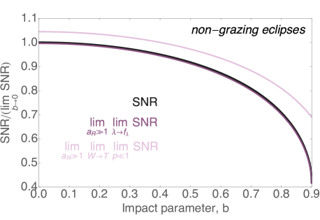
In the case of a grazing event, we formally need to use the $\lambda$ function defined earlier in Equation (12):

$$\lim_{a_{R}\gg 1}\mathrm{SNR}_{\mathrm{multi}}^{\text{grazing}}=\frac{\nu_{\mathrm{multi}}}{2}((1+p)^{2}-b^{2})^{1/4}\lambda.$$ (31)

The $\lambda$ function (Equation 12) can be approximated to high accuracy using the $f_{\lambda}$ derived in Appendix A (see Equation 54). Using this approximation, we may write

$$\lim_{a_{R}\gg 1}\lim_{\lambda\to f_{\lambda}}\mathrm{SNR}_{\mathrm{multi}}^{\text{grazing}}= \frac{\nu_{\mathrm{multi}}}{2}((1+p)^{2}-b^{2})^{1/4}$$

$$\frac{(1+p-b)^{2}}{4}\Bigg{(}1-2\log_{4}\Big{[}\frac{1+p-b}{2p}\Big{]}\Bigg{)}.$$ (32)

As shown in Fig. 3, this approximation provides an excellent match to the true function with a considerably simpler form than that of the $\lambda$ function.

Figure 3: Comparison of three approximations (coloured lines) to the full SNR expression (black) for grazing transits. We here adopt $p=0.1$, $P=3$ d, $a_{R}=10$, $e=0.1$ and $\omega=0$. The most approximate form (Equation 19) poorly reproduces the shape, but assuming $a_{R}\gg 1$ and $\lambda\to f_{\lambda}$ (Equation 31) provides an excellent approximation.

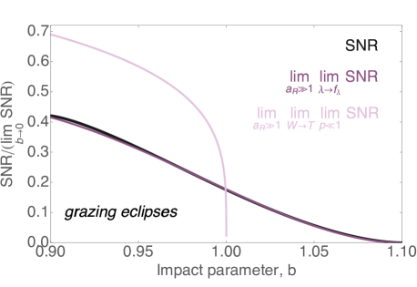
As expected, Equations (30) and (32) are equivalent in the limit of $b\to(1-p)$, meaning that these two functions join together at the boundary dividing them.

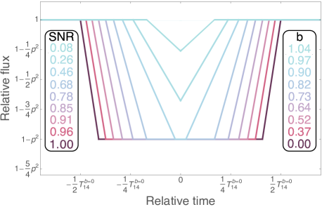
In Fig. 4, we plot a sample of trapezoidal light curves following our model, with the associated $b$ and $\mathrm{SNR}_{\mathrm{single}}$ values listed as a visual guide.

Figure 4: Examples of the trapezoidal transits following our model (colored lines). The adopted parameters are those of a typical hot Jupiter, except for $b$, which is evenly spaced in $(1-b^{2})$ space. For each example transit, we list both the $b$ value and the associated $\mathrm{SNR}_{\mathrm{single}}$ (relative to the $b=0$ case).

4.2 Updated joint conditional probability distribution

The joint probability distribution of the transit parameters, conditioned upon the fact that a planet transits and the transit is detectable, is directly proportional to the SNR, as shown in Equations (21) and (25). As before then, the joint probability may be expressed as

$$\mathrm{Pr}(\boldsymbol{\Theta}|\hat{d},\hat{b})\propto\mathrm{Pr}(\hat{d},\hat{b}|\boldsymbol{\Theta})\mathrm{Pr}(\boldsymbol{\Theta}).$$ (33)

The $\mathrm{Pr}(\hat{d},\hat{b}|\boldsymbol{\Theta})$ represents the observational bias, which using the simpler approximation in §3 was given by Equation (27). Now, the form of $\mathrm{Pr}(\hat{d},\hat{b}|\boldsymbol{\Theta})$ is modified to account for the trapezoidal shape of the transit, but the only terms which have been changed relate to $p$ and $b$.

As an additional improvement, we modify the geometric bias (Equation 23) to include grazing events, such that transits are now defined as $b<1+p$. Following the methodology described in Kipping (2014), it may be shown that this modifies $\mathrm{Pr}(\hat{b}|\boldsymbol{\Theta})\to(1+p)\mathrm{Pr}(\hat{b}|\boldsymbol{\Theta})$.

Accordingly, we may express the observational bias as

$$\mathrm{Pr}(\hat{d},\hat{b}|\boldsymbol{\Theta})\propto\kappa\times\left\{\begin{array}[]{ll}\eta(p,b)&0\leq b<1-p\\ \zeta(p,b)&1-p\leq b<1+p\\ 0&1+p\leq b<\infty\end{array}\right.,$$ (34)

where $\kappa$ is defined in Equation (28), and

$$\eta(p,b)\equiv \tfrac{1}{2}(1+p)((1+p)^{2}-b^{2})^{-1/4}p^{2}$$

$$\Big{(}\sqrt{(1+p)^{2}-b^{2}}+\sqrt{(1-p)^{2}-b^{2}}\Big{)},$$ (35)

$$\zeta(p,b)\equiv \tfrac{1}{2}(1+p)((1+p)^{2}-b^{2})^{1/4}\frac{(1+p-b)^{2}}{4}$$

$$\Bigg{(}1-2\log_{4}\Big{[}\frac{1+p-b}{2p}\Big{]}\Bigg{)}.$$ (36)

In the above, a Taylor series expansion in small $p$ provides a first-order leading term equal to that of Equation (27), demonstrating the equivalency of the two derivations.

4.3 Marginalized distributions

We first note that, as in the simple case, the observational bias terms are largely separable, with the exceptions of $e$ and $\omega$, and now $p$ and $b$, being covariant:

$$\mathrm{Pr}(\hat{d},\hat{b}|\boldsymbol{\Theta}) \propto\mathrm{Pr}(\hat{d},\hat{b}|P)\mathrm{Pr}(\hat{d},\hat{b}|e,\omega)\mathrm{Pr}(\hat{d},\hat{b}|b,p).$$ (37)

If we further assume that the intrinsic distributions are fully separable, then the above simplifies the derivation of marginalized distributions, since we can write, for example,

$$\mathrm{Pr}(P|\hat{d},\hat{b}) \propto\int\int\int\int\int\mathrm{Pr}(\hat{d},\hat{b}|\boldsymbol{\Theta})\mathrm{Pr}(\boldsymbol{\Theta})\,\mathrm{d}p\,\mathrm{d}b\,\mathrm{d}\rho_{\star}\,\mathrm{d}e\,\mathrm{d}\omega$$

$$\propto\mathrm{Pr}(\hat{d},\hat{b}|P)\mathrm{Pr}(P),$$ (38)

where in the case of the above, adopting a log-uniform intrinsic period distribution ($\propto P^{-1}$), would mean that $\mathrm{Pr}(P|\hat{d},\hat{b})\propto P^{-2}$. Repeating this marginalization for the other terms allows us to write

$$\mathrm{Pr}(P|\hat{d},\hat{b}) \propto P^{-1}\mathrm{Pr}(P),$$ (39)

$$\mathrm{Pr}(\rho_{\star}|\hat{d},\hat{b}) \propto\rho_{\star}^{-1/2}\mathrm{Pr}(\rho_{\star}),$$ (40)

$$\mathrm{Pr}(e,\omega|\hat{d},\hat{b}) \propto\frac{(1+e\sin\omega)^{1/2}}{(1-e^{2})^{3/4}}\mathrm{Pr}(e)\mathrm{Pr}(\omega),$$ (41)

$$\mathrm{Pr}(b,p|\hat{d},\hat{b}) \propto\mathrm{Pr}(\hat{d},\hat{b}|b,p)\mathrm{Pr}(b)\mathrm{Pr}(p),$$ (42)

where we do not write out the last function due to its split-domain nature (see Sections 4.3.1 and 4.3.2 for discussion). First, though, note that we do not impose specific intrinsic priors in the above, allowing for flexibility in their usage. The only critical assumption in deriving the above is that the intrinsic distributions are separable.

4.3.1 The case of $p$

In the case of the simple priors derived earlier, $p$ and $b$ are separable, in which case one can show that

$$\mathrm{Pr}(b|\hat{d},\hat{b}) \propto(1-b^{2})^{1/4}\mathrm{Pr}(b),$$ (43)

$$\mathrm{Pr}(p|\hat{d},\hat{b}) \propto p^{2}\mathrm{Pr}(p).$$ (44)

The latter expression reflects our intuition that detected transits are biased towards larger planets with a quadratic scaling. The bias evident in $\mathrm{Pr}(b|\hat{d},\hat{b})$ is likely unfamiliar to the reader, but we show later in Fig. 8 that it provides a good match to observations.

For the more advanced case, calculating the one-dimensional marginalized $\mathrm{Pr}(p|\hat{d},\hat{b})$ and $\mathrm{Pr}(b|\hat{d},\hat{b})$ can only be accomplished by assuming an intrinsic distribution for $\mathrm{Pr}(p)$ and $\mathrm{Pr}(b)$. For impact parameter $b$, a uniform prior is reasonable and expected, but $p$ is somewhat non-trivial. Before tackling this issue, though, the fact that we can define $\mathrm{Pr}(b)$ means we can marginalize it out to derive $\mathrm{Pr}(p|\hat{d},\hat{b})$. Doing so leads to a highly elaborate expression (which cannot be compactly written out here) involving generalized hypergeometric functions.

Figure 5: Red line shows the analytic (but highly elaborate) functional dependence of $\mathrm{Pr}(\hat{d},\hat{b}|p)$ with respect to $p$, which is clearly super-quadratic (grey line) and very well approximated by a power law of index $5/2$ (black line). The pink line shows the full function in the case where V-shaped (i.e., grazing) transits are not considered ‘detections.’

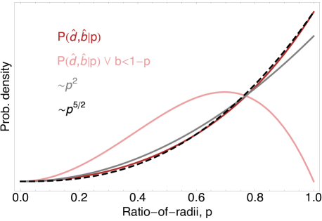
Plotting our solved function $\mathrm{Pr}(p|\hat{d},\hat{b})$ (which is purely dependent on $p$) in Fig. 5 reveals that the function is super-quadratic with respect to $p$. This implies that if one assumed a detection bias of $p^{2}$, one would underestimate the true number of small planets, since the bias towards $p$ is actually sharper. Additionally, we observe that the plotted function closely resembles a power-law, for which we can fit the index. We therefore approximate

$$\mathrm{Pr}(p|\hat{d},\hat{b}) \propto p^{\alpha}\mathrm{Pr}(p).$$ (45)

A least-squares fit of samples suggests $\alpha=2.424$, but plotting even $\alpha=5/2$ reveals excellent agreement. It is important to stress that this value is not dependent upon any assumption regarding the intrinsic distributions, except that impact parameter is uniformly distributed and separable from $p$. Under this assumption, and the assumption that detectability is proportional to SNR, geometric effects conspire to favour the detection of planets with a scaling of $p^{5/2}$. We also tried repeating the derivation marginalizing over only $b<1-p$, which is equivalent to insisting that V-shaped transits are not considered ‘detections.’ This line, plotted in pink in Fig. 5, reveals a turn-over at $p=0.696$, since it is increasingly unlikely for the disc of a large planet to fully pass in front of the star.

4.3.2 The case of $b$

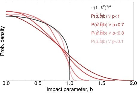
We are unable to derive a closed-form expression for the marginalized distribution of $\mathrm{Pr}(b|\hat{d},\hat{b})$. Instead, we perform the integral numerically over a grid of $b$ values in order to plot the functional form of the expression. For this calculation, we assume that the logarithm of $p$ is distributed uniformly from $10^{-3}$ to a fixed upper limit, which we try varying.

The results, shown in Fig. 6, illustrate that the functional form is generally flat at low $b$ and follows the approximate shape of the simple form derived earlier (i.e. $(1-b^{2})^{1/4}$). The effect of the $p$ marginalization largely appears to be that of a convolution kernel, smoothing out the distribution.

Figure 6: Coloured lines show the analytic (but highly elaborate) functional dependence of $\mathrm{Pr}(\hat{d},\hat{b}|b)$ with respect to $b$, the observational bias to transit impact parameter. The black line shows the same bias derived in the small-planet ($p\to 0$) limit of a box-like transit.

4.3.3 The case of $e$

For eccentricity and argument of periastron, we assume that $\omega$ has a uniform intrinsic distribution. Regardless of the intrinsic distribution for $e$, we find that marginalizing over $\omega$ is possible analytically, as

$$\mathrm{Pr}(e|\hat{d},\hat{b}) \propto\mathrm{Pr}(e)\int_{\omega=0}^{2\pi}\mathrm{Pr}(e,\omega|\hat{d},\hat{b})\mathrm{Pr}(\omega)\,\mathrm{d}\omega,$$ (46)

giving

$$\mathrm{Pr}(e|\hat{d},\hat{b}) \propto\frac{\mathrm{Pr}(e)}{(1-e^{2})^{3/4}}\Bigg{(}\sqrt{1-e}E\Big{[}\frac{2e}{e-1}\Big{]}+\sqrt{1+e}E\Big{[}\frac{2e}{e+1}\Big{]}\Bigg{)},$$ (47)

where $E(x)$ is the complete elliptic integral of $x$. The above is essentially an exponential-like function multiplied by the intrinsic $e$ prior and thus distorts the observed eccentricity distribution towards more elliptical orbits than the true underlying distribution.

4.3.4 The case of $\omega$

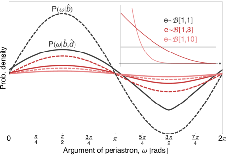
Repeating this trick for $\omega$ is more challenging and is functionally dependent upon the assumed form for $\mathrm{Pr}(e)$. In what follows, we adopt a Beta distribution for $e$, for reasons discussed in Kipping (2013). Whilst a closed-form expression was not found, numerically marginalizing over $e$ for three different choices of the Beta shape parameters allows us to visualize the effect of the detection bias, as shown in Fig. 7.

In this figure, we compare the results of including both detection bias and geometric bias (this work), versus the geometric bias alone (expressions of Kipping 2014). It is clear that our expressions significantly suppress the $\omega$ biases, leading to a population more evenly distributed with respect to $\omega$. This can be understood by considering that apoastron transits, whilst geometrically disfavoured, have a significant detection enhancement due to their longer transit durations.

Figure 7: Solid coloured lines show $\mathrm{Pr}(\omega|\hat{d},\hat{b})$, whereas dashed lines show $\mathrm{Pr}(\omega|\hat{b})$ for comparison, using the same inputs. Including detection bias suppresses the strong bias towards periastron transits.

5 Discussion

In this work, we have derived the joint probability distribution of the basic transit parameters conditioned upon two observational biases affecting this type of measurement: geometric bias and detection bias. By treating the transit as a trapezoid, accounting for grazing events, and using conditional probability theory, we have derived an analytic, closed form for these biases (see Equation 34).

Whereas previous works have used analytic arguments to predict the detection yields of transit surveys subject to observational biases (e.g. Beatty & Gaudi 2008), the focus here is the distortion of the observed transit parameter distributions away from those of the underlying exoplanet population. Inferences about the properties of Kepler planets are strongly affected by geometric and detection bias, and our work provides a general framework to interpret the observed trends.

Our work is not intended to replace numerical Monte Carlo simulations, which typically perform injection/recovery tests through a detection pipeline (e.g. see Petigura et al. 2013; Christiansen et al. 2015; Dressing & Charbonneau 2015). These results, tailored to a specific mission, have both advantages in their flexibility and disadvantages in obscuring the mechanisms responsible for various trends. In this sense, our work complements numerical efforts by providing insight into what observational trends are inherent to the transit technique, rather than effects localized to a particular survey. We highlight here several important results from our work.

We predict that observational bias should lead to a non-uniform distribution in the impact parameters of detected transiting planets. This prediction may be tested with the Kepler catalogue, for which we turn to Swift et al. (2015), who derived homogeneous posterior distributions for the basic transit parameters, including $b$, of 163 Kepler planetary candidates. The cumulative distributions of these terms are shown in fig. 9 of that work, of which we reproduce a version in Fig. 8 here.

Figure 8: Distribution of the transit impact parameter for the sample of Kepler planetary candidates studied in Swift et al. (2015). The measured distribution (green) is reasonably well approximated by the (simple case) prior $\mathrm{Pr}(b|\hat{d},\hat{b})$ of Equation (27) derived in this work.

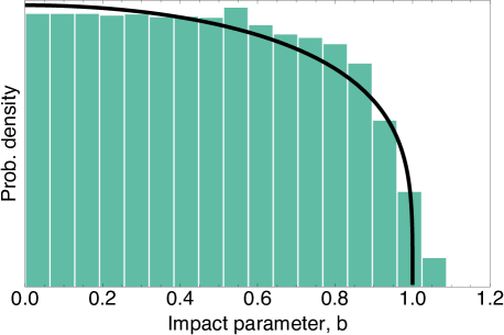
Despite the fact that Swift et al. (2015) impose a uniform prior on $b$, the overall distribution drops off at high $b$, reproducing our expectation that such cases are indeed less frequent in a SNR-limited survey like Kepler. Fig. 8 compares the measured distribution to that predicted by our function $\mathrm{Pr}(b|\hat{d},\hat{b})$ in the simple case of Equation (27), which displays a reasonable match to the observed shape.

Aside from providing an explanation for the distribution of impact parameters observed in real data (Swift et al., 2015), we highlight two other important results from our work. First, we update the well-known eccentricity bias of transits (Barnes 2007; Burke 2008; Kipping 2014) to include detection bias. We find that the previously reported bias of transiting planets towards being preferentially near periastron is substantially relaxed by virtue of near-apoastron transits being much longer and thus more detectable. Equation (47) provides a general formulation to correct for the eccentricity bias for any assumed intrinsic distribution.

Finally, we highlight that we find the observational bias of transits with respect to the ratio-of-radii, $p$, is not quadratic (i.e. $p^{2}$), as commonly assumed, but actually super-quadratic and well-approximated by $p^{5/2}$ (see Fig. 5 and Section 4.3.1). Critically, this result is independent of any assumption about the intrinsic distribution of $p$ and only assumes that impact parameter is intrinsically uniformly distributed. This result is driven by larger planets having (i) a longer transit duration and (ii) a higher geometric transit probability. Excluding grazing events (i.e. assuming $b<1-p$) leads to a non-monotonic form for the bias with respect to $p$. These results highlight the importance of correctly accounting for observational biases in statistical calculations seeking to infer the true planetary radius distribution.

Appendix A An Approximation for $\lambda$

The expression for $\lambda$ (Equation 12) is restrictive for further analytic work, and thus we seek an approximation via a simple polynomial, aiming to capture both the curvature and boundary conditions of the function. We consider using a so-called smooth-step function, $f[x]$, over the interval $0<x<1$, where $f[x]$ varies smoothly from $f[0]=0$ to $f[1]=1$. The function $\lambda$ is approximated by

$$\lambda \simeq p^{2}f[\mathcal{S}^{\prime}],$$

$$\mathcal{S}^{\prime} =\frac{1+p-\mathcal{S}}{2p}.$$ (48)

The simplest function we might propose is $f_{1}[x]=x$, which is simply a straight line. A common smooth-step function used in computer graphics is

$$f_{2}[x]=3x^{2}-2x^{3}.$$ (49)

Several other smooth-step functions exist at higher order, such as

$$f_{3}[x] =6x^{5}-15x^{4}+10x^{3},$$ (50)

$$f_{4}[x] =-20x^{7}+70x^{6}-84x^{5}+35x^{4}.$$ (51)

Figure 9: Comparison of several “smooth-step” approximations to the $\lambda$ function. Our newly derived function, $f_{\lambda}$, provides an excellent match.

Plotting these functions in Fig. 9, it apparent that the true function, $\lambda$, lies between $f_{1}[\mathcal{S}^{\prime}]$ and $f_{2}[\mathcal{S}^{\prime}]$. We therefore seek to generalize the $f_{2}[\mathcal{S}^{\prime}]$ expression by writing:

$$f_{\lambda}[x]=(\alpha+1)x^{\beta}-\alpha x^{\gamma}.$$ (52)

We note that the $\lambda$ function intersects $\frac{1}{2}$ for $\lim_{p\to 0}\lambda(p,1)=\frac{1}{2}$, which implies that we expect $f_{\lambda}[\frac{1}{2}]=\frac{1}{2}$. Imposing the above and solving for $\alpha$ allows us to replace

$$\alpha =-\frac{2^{\gamma-1}(2^{\beta}-2)}{2^{\beta}-2^{\gamma}}.$$ (53)

Experimenting with different low-integer combinations of $\beta$ and $\gamma$, we find that setting $\beta=\gamma=2$ yields a close match. Indeed, setting $\beta=\gamma$ and applying a least squares fit for $\beta$ yields $\beta=2$. Adopting this value, we therefore use the following approximate expression for $\lambda$ (plotted in Fig. 9):

$$f_{\lambda}[x] =x^{2}(1-\log_{4}x^{2}).$$ (54)

References

- Barnes (2007) Barnes, J. W., 2007, PASP, 119, 986
- Beatty & Gaudi (2008) Beatty, T. G. & Gaudi, S. B., 2008, ApJ, 686, 1302
- Burke (2008) Burke, C. J., 2008, ApJ, 679, 1566
- Burke et al. (2015) Burke, C. J. et al., 2015, ApJ, 809, 8
- Carter et al. (2008) Carter, J. A., Yee, J. C., Eastman, J., Scott, S. B. & Winn, J. N., 2008, ApJ, 689, 499
- Christiansen et al. (2015) Christiansen, J. L. et al., 2015, ApJ, 810, 95
- Dalcanton et al. (2015) Dalcanton, J. et al., 2015, preprint (arXiv:1507.04779)
- Dressing & Charbonneau (2015) Dressing, C. D. & Charbonneau, D., 2015, ApJ, 807, 45
- Fressin et al. (2013) Fressin, F. et al., 2013, ApJ, 766, 81
- Jenkins et al. (2010) Jenkins, J. M. et al., 2010, ApJ, 713, 87
- Kipping (2010) Kipping, D. M., 2010, MNRAS, 407, 301
- Kipping (2013) Kipping, D. M., 2013, MNRAS, 434, L51
- Kipping (2014) Kipping, D. M., 2014, MNRAS, 444, 2263
- Mandel & Agol (2002) Mandel, K. & Agol, E., 2002, ApJ, 580, 171
- Petigura et al. (2013) Petigura, E. A., Howard, A. W. & Marcy, G. W., 2013, PNAS, 110, 19273
- Swift et al. (2015) Swift, J. J., Montet, B. T., Vanderburg, A., Morton, T., Muirhead, P. S. & Johnson, J. A., 2015, ApJ, 218, 26
Appendix A An Approximation for
The expression for (Equation 12) is restrictive for further analytic work, and thus we seek an approximation via a simple polynomial, aiming to capture both the curvature and boundary conditions of the function. We consider using a so-called smooth-step function, , over the interval , where varies smoothly from to . The function is approximated by