For quantum field theories with topological sectors, Monte Carlo simulations on fine lattices tend to be obstructed by an extremely long auto-correlation time with respect to the topological charge. Then reliable numerical measurements are feasible only within individual sectors. The challenge is to assemble such restricted measurements in a way that leads to a substantiated approximation to the fully fledged result, which would correspond to the correct sampling over the entire set of configurations. We test an approach for such a topological summation, which was suggested by Brower, Chandrasekharan, Negele and Wiese. Under suitable conditions, energy levels and susceptibilities can be obtained to a good accuracy, as we demonstrate for O($N$) models, SU(2) Yang-Mills theory, and for the Schwinger model.

1 Motivation

We consider quantum field theories with topological sectors, in Euclidean spacetime. These sectors are characterized by a topological charge $Q\in\mathbb{Z}$, which is a functional of the field configuration. In infinite volume, the configurations with finite action are divided into these disjoint sectors. The same property holds in finite volume with periodic boundary conditions.

Examples are O$(N)$ models in $d=N-1$ dimensions, all 2d CP$(N-1)$ models, 4d SU$(N)$ Yang-Mills gauge theories ($N\geq 2$), as well as QCD, and 2d U(1) gauge theory, as well as the Schwinger model. In all these models, a continuous deformation of a given configuration (at finite action) can only lead to configurations within the same topological sector, i.e. the deformation cannot alter the topological charge $Q$.

In light of this definition, lattice regularized models have in general no topological sectors — strictly speaking. Nevertheless, it is often useful to divide the set of lattice field configurations into sectors, which turn into the topological sectors in the continuum limit. The definition of a topological charge on the lattice is somewhat arbitrary. In presence of chiral fermions (where the lattice Dirac operator obeys the Ginsparg-Wilson relation), the fermion index provides a sound formulation [1]. For the O$(N)$ models the geometric definition [2] is optimal, since it guarantees integer topological charges on periodic lattices (for all configurations except for a subset of measure zero). In gauge theory, field theoretic definitions are often applied, usually combined with smearing or cooling techniques, see e.g. Ref. [3]. These techniques are computationally cheap and provide, on fine lattices or at fixed topology, results which agree well with the computationally demanding fermion index [4, 5, 6].

As we proceed to finer and finer lattices, the formulation becomes more continuum-like, and changing a (suitably defined) topological sector of the lattice field is getting more and more tedious — for this purpose, continuous deformations have to pass through a statistically suppressed domain of high Euclidean action. To a large extent, this property persists for finite but small deformations, as they are carried out in the Markov chain of a Monte Carlo simulation which performs small update steps.

In QCD simulations with dynamical quarks, the gauge configurations are usually generated with a Hybrid Monte Carlo (HMC) algorithm, with small updates, on lattices of a spacing $a$ in the range $0.05~{}{\rm fm}\raisebox{-2.15277pt}{$\,\stackrel{{\scriptstyle<}}{{\scriptstyle\sim}}\,$}a\raisebox{-2.15277pt}{$\,\stackrel{{\scriptstyle<}}{{\scriptstyle\sim}}\,$}0.15~{}{\rm fm}$. The artifacts due to the finite lattice spacing tend to be the main source of systematic errors. Therefore, the lattice community will try to suppress them further by proceeding to even finer lattices, $a<0.05~{}{\rm fm}$.

This will provide continuum-like features, which are highly welcome in general, but as a draw-back it will become harder to change the topological sector. A HMC simulation may well be trapped in a single sector over a tremendously long trajectory; in particular, this is the experience in QCD simulations with dynamical overlap quarks [7]. In this case, Ref. [8] suggested a method to estimate the ratio between topologically constrained partition functions, and tested this method by determining the topological susceptibility from fixed topology overlap quark simulations.

In some circumstances it is even motivated to suppress topological transitions on purpose, in particular when dealing with dynamical chiral fermions. In that context, configurations in a transition region cause technical problems, like a bad condition number of an overlap or domain wall Dirac operator. This can be avoided by the use of unconventional lattice gauge actions, known as “topology conserving gauge actions” [9, 4] (see also Ref. [10] for a very similar formulation).

A further option is the use of a “mixed action”, where one implements chiral symmetry only for the valence quarks, which requires just a moderate computational effort. In particular, overlap valence quarks have been combined with Wilson sea quarks. However, in this set-up the continuum limit is not on safe ground, because (approximate) valence quark zero modes are not compensated by the sea quark spectrum [11]. This problem might be avoided by fixing the topological sector particularly to $Q=0$.

In such settings, there are obvious questions about the (effective) ergodicity of the algorithm, since the simulation does not sample properly the entire space of all configurations. Even if we ignore this conceptual question, in practice the measurement of an observable may well be distorted. This is the issue to be addressed in this work.

Section 2 describes the Brower-Chandrasekharan-Negele-Wiese (BCNW) approach, and Sections 3 and 4 probe it in the 1d O(2) and the 2d O(3) non-linear $\sigma$-model. It is explored further in 4d SU(2) Yang-Mills theory in Section 5, and in the Schwinger model in Section 6. The field theoretic models discussed in Sections 4 to 6 share fundamental features with QCD. Section 7 is devoted to our conclusions.

2 The BCNW method

As a remedy against the topological freezing of Monte Carlo histories, Lüscher suggested the use of open boundary conditions, such that the topological charge can change continuously [12]. This overcomes the problem, but it breaks translational invariance and one gives up integer topological charges $Q$. However, $Q\in\mathbb{Z}$ provides a valuable link to aspects, which are analytically known or conjectured in the continuum, for instance regarding the $\epsilon$-regime of QCD, or properties based on an instanton picture. Therefore it is still motivated to also explore alternative approaches.

In this work we maintain periodic boundary conditions (in some volume $V$) for the bosonic fields involved, so the topological charges $Q$ are integers. Moreover we consider models with parity invariance. This implies $\langle Q\rangle=0$, and the topological susceptibility is given by

$$\chi_{\rm t}=\frac{1}{V}\langle Q^{2}\rangle\ .$$ (2.1)

In this framework, we are going to test the BCNW approximation [14]. It can be written in the form of an expansion in inverse powers of $V\chi_{\rm t}$,

$$\langle{\cal O}\rangle_{Q}\simeq\langle{\cal O}\rangle+\frac{1}{V\chi_{\rm t}}c+\frac{1}{(V\chi_{\rm t})^{2}}(\bar{c}-c\,Q^{2})-\frac{2}{(V\chi_{\rm t})^{3}}\bar{c}\,Q^{2}\ .$$ (2.2)

The left-hand-side refers to the expectation value of some observable ${\cal O}$ (Refs. [14] inserted specifically the pion mass) within the sectors of topological charges $\pm Q$. It is accessible even in simulations which are confined to one — or a few — topological sectors.

All the unknown terms on the right-hand-side, i.e. the expectation value $\langle{\cal O}\rangle$, $\chi_{\rm t}$ and the coefficients $c$ and $\bar{c}$, are quantities that asymptotically stabilize in large volume. Hence this form enables the use of results for $\langle{\cal O}\rangle_{Q}$, measured in several volumes and for distinct $|Q|$, to determine these unknown terms. In particular we are interested in $\langle{\cal O}\rangle$ and $\chi_{\rm t}$. The coefficients are determined as well; for instance $c$ can be expressed by derivatives with respect to the vacuum angle $\theta$ of the extended Euclidean action $S+{\rm i}\theta Q$,

$$c=\frac{1}{2}\langle{\cal O}\rangle^{\prime\prime}(\theta)|_{\theta=0}\ ,$$ (2.3)

but we are not going to discuss any conceivable interpretation of these coefficients.

Actually the third order in approximation (2.2) is incomplete, but the additional term in this order would bring along another free parameter. These terms are identified and discussed in detail in Refs. [15, 16, 17]. Here we mostly focus on the simplest form which captures the $Q$-dependence of $\langle{\cal O}\rangle_{Q}$, and which involves only three parameters (though an incomplete second order),

$$\langle{\cal O}\rangle_{Q}\approx\langle{\cal O}\rangle+\frac{c}{V\chi_{\rm t}}\left(1-\frac{Q^{2}}{V\chi_{\rm t}}\right)\ .$$ (2.4)

In the following, we will refer to this approximation as the BCNW formula. Obviously we cannot determine the quantities $\langle{\cal O}\rangle$, $\chi_{\rm t}$ and $c$ within a single volume; for instance

$$\langle{\cal O}\rangle_{Q_{1}}-\langle{\cal O}\rangle_{Q_{2}}\approx\frac{c}{(V\chi_{\rm t})^{2}}(Q_{2}^{2}-Q_{1}^{2})$$ (2.5)

only determines the ratio $c/\chi_{\rm t}^{2}$. If we include different volumes $V_{1}$ and $V_{2}$, however, we could use e.g. $\langle{\cal O}\rangle_{0}(V_{1})-\langle{\cal O}\rangle_{0}(V_{2})\approx\frac{c}{\chi_{\rm t}}(1/V_{1}-1/V_{2})$ to fix $c/\chi_{\rm t}$, and we obtain — along with relation (2.5) — all three quantities, $\langle{\cal O}\rangle$, $\chi_{\rm t}$ and $c$ (we repeat that only the former two are of interest). In practice one would rather involve several volumes and topological sectors, and perform a 3-parameter fit to the (over-determined) system.

We distinguish three regimes for the volume $V$

• Small volume: there are significant finite size effects of the ordinary type, not related to topology fixing, in particular in $\langle{\cal O}\rangle$ and $\chi_{\rm t}$.

• Moderate volume: ordinary finite size effects are negligible (they tend to be exponentially suppressed), but $\langle{\cal O}\rangle_{Q}$ still depends significantly on $|Q|$ and $V$.

• Large volume: there are hardly any finite size effects left, even the correction terms in approximations (2.2), (2.4) are negligible.

In small volumes, the formulae (2.2) and (2.4) cannot be applied, because results from various volumes cannot be used for the same fit. In large volumes, we obtain the correct value for $\langle{\cal O}\rangle$ anyhow, without worrying about frozen topology, as we see from the expansions (2.2) and (2.4). However, such large volumes may be inaccessible in realistic simulations, due to limitations of the computational resources. Hence we are interested in moderate volumes, where the determination of $\langle{\cal O}\rangle$ is difficult, but possibly feasible by means of the BCNW approximation. Moreover, that regime also provides an estimate for $\chi_{\rm t}$, which is particularly hard to measure directly.

The derivation of formula (2.2) involves approximations, which assume:

• $\langle Q^{2}\rangle=V\chi_{\rm t}$ is large. As we mentioned before, eq. (2.2) takes the form of an expansion in $1/\langle Q^{2}\rangle$. Once $\chi_{\rm t}$ is stable, this can also be viewed as a large volume expansion.

• $|Q|/\langle Q^{2}\rangle$ is small, so we should work in the sectors with a small absolute value $|Q|$. This is less obvious from the formulae (2.2) and (2.4) (although the terms $\propto Q^{2}$ are related to this condition), but it is required for a step in its derivation, which relies on a stationary phase approximation.

Here we employ numerical data to explore how large $\langle Q^{2}\rangle$ has to be for this approximation to be sensible, and up to which absolute value $|Q|$ the data are useful in this context. In practice it is rather easy to work at small $|Q|$, but the former condition could be a serious obstacle.

So far there have been only few attempts to apply this approximation to simulation data. This was done for the 2-flavor Schwinger model with dynamical overlap fermions [19, 20] with respect to the pseudo-scalar mass $M_{\pi}$ and the chiral condensate $\Sigma$. Tests for a quantum rotor — more precisely a scalar particle on a circle with a potential — are reported in Refs. [15, 16].

Another approach was derived — similarly to the BCNW approximation — in Ref. [21]. It refers to the long-distance correlation of the topological charge density $q(x)$, $Q=\int d^{d}x\,q(x)$. The applicability of that method has been tested in a set of models [22], and variants had been studied previously [23]. Further approaches to extract physics from topologically frozen Markov chains include Refs. [24, 25, 26]. Preliminary results of this work have been anticipated in some proceeding contributions [15, 17, 18, 27].

3 Tests for the quantum rotor

As a simple but precise test, we first consider a toy model from quantum mechanics (i.e. 1d quantum field theory), namely the quantum rotor, or 1d XY model, or 1d O(2) model. It describes a free quantum mechanical particle moving on a circle, with a periodicity condition in Euclidean time. A theoretical discussion of this system, in the continuum and for different lattice actions, is given in Ref. [28]. Below we write down the continuum action, and on the lattice the standard action and the Manton action [30] (in lattice units),

$$S_{\rm cont}[\varphi] = \frac{\beta_{\rm cont}}{2}\int_{0}^{L_{\rm cont}}dt\,\dot{\varphi}(t)^{2}\ ,$$

$$S_{\rm standard}[\varphi] = \beta\sum_{t=1}^{L}\Big{(}1-\cos(\Delta\varphi_{t})\Big{)}\ ,$$

$$S_{\rm Manton}[\varphi] = \frac{\beta}{2}\sum_{t=1}^{L}\,(\Delta\varphi_{t})^{2}\ .$$ (3.1)

$L_{\rm cont}$ and $L$ are the extent of the periodic Euclidean time interval in the continuum and on the lattice, respectively, $\varphi(t)$ and $\varphi_{t}$ are time dependent angles, with $\varphi(L_{\rm cont}+t)=\varphi(t)$, $\varphi_{L+t}=\varphi_{t}$. $\beta_{\rm cont}$ and $\beta$ can be interpreted as an inverse temperature, or in this case also as the moment of inertia. In the terms for the lattice actions we define

$$\Delta\varphi_{t}=(\varphi_{t+1}-\varphi_{t})\ {\rm mod}\ 2\pi\in(-\pi,\pi]\ ,$$ (3.2)

i.e. the modulo function is implemented such that it minimizes $|\Delta\varphi_{t}|$. Thus $\Delta\varphi_{t}$ also defines the lattice topological charge density $q_{t}$ (geometric definition) and the charge $Q$,

$$q_{t}=\frac{1}{2\pi}\Delta\varphi_{t}\ ,\quad Q[\varphi]=\sum_{t=1}^{L}q_{t}\in\mathbb{Z}\ .$$ (3.3)

In the continuum and infinite size $L_{\rm cont}$, the correlation length and its product with the topological susceptibility amount to

$$\xi_{\rm cont}=2\beta_{\rm cont}\ ,\quad\chi_{\rm t}\ \xi_{\rm cont}=\frac{1}{2\pi^{2}}\ .$$ (3.4)

Analytic expressions for the corresponding quantities on the lattice, with the standard action and the Manton action, are given in Ref. [28].

Our simulations were carried out with the Wolff cluster algorithm [31], which performs non-local update steps. This algorithm is highly efficient and provided a statistics of $5\times 10^{9}$ measurements for each setting. Since it changes the topological sector frequently, in this case the observables could also be measured directly to high precision, which allows for a detailed test of the BCNW method. In most quantum field theoretic models no efficient cluster algorithm is known, in particular in the presence of gauge fields. Then one has to resort to local update algorithms, which motivates this project, as we pointed out in Section 1.

For our tests we set $\beta=4$ and consider six lattice sizes in the range $L=150\dots 400$. This is large compared to the correlation length, which was measured at $L=400$ as

$$\xi_{\rm standard}=6.81495(4)\ ,\quad\xi_{\rm Manton}=7.9989(1)\ ,$$ (3.5)

very close to the analytic values at $L=\infty$. This demonstrates that ordinary finite size effects are very small, but — as we are going to see — there are significant fixed topology finite size effects. Hence we are in the regime of moderate volumes, as desired. Moreover, this regime is sensible also because lattice artifacts are quite well suppressed.

The BCNW formula consists of leading terms in an expansion in $1/\langle Q^{2}\rangle$, cf. Section 1. In the range $L=150\dots 400$ we obtain

$$\langle Q^{2}\rangle_{\rm standard}=1.13\dots 3.02\ ,\quad\langle Q^{2}\rangle_{\rm Manton}=0.95\dots 2.53\ .$$ (3.6)

This suggests that we are in the transition regime to the validity of this method, which is interesting to explore.

3.1 Action density

We first consider the action density

$$s=\langle S\rangle/V\ .$$ (3.7)

This quantity is not directly physical, but it is suitable for testing the BCNW method, based on topologically restricted expectation values $s_{|Q|}=\langle S\rangle_{|Q|}/V$. Moreover, the corresponding fits provide a value for $\chi_{\rm t}$, which is physical.

Figure 1 shows the action density for both lattice actions under consideration, measured at fixed $|Q|=0\dots 4$, and by including all sectors (the way the simulation samples them). The latter is constant to high accuracy for $L=150\dots 400$, which confirms that ordinary finite size effects are negligible. On the other hand, at fixed $|Q|$ we see deviations far beyond the statistical errors, depending on $L$ and $|Q|$, so this setting is appropriate for the application of the BCNW method.

Figure 1: The action density in the 1d O(2) model at $\beta=4$ on lattices of size $L=150\dots 400$, with the standard action (left) and the Manton action (right). We show $s$ measured in all sectors (which is practically constant in this range of $L$), as well as the values of $s_{|Q|}$ in the sectors $|Q|=0\dots 4$, which strongly depend on $|Q|$ and $V$.

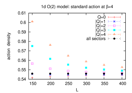
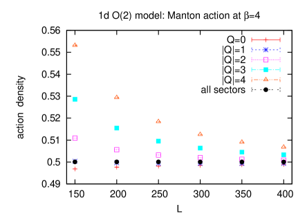
Table 1 presents our results obtained by least-square fits to the BCNW approximation (2.4): we use data for $s_{|Q|}$ in all six volumes, and in the topological sectors $|Q|=0\dots|Q|_{\rm max}$, where $|Q|_{\rm max}$ varies from 1 to 4. Similar results are obtained when we only involve the larger volumes, such as $L=250\dots 400$ or $300\dots 400$.

	standard action		Manton action
$|Q|_{\rm max}$	$s$	$\chi_{\rm t}$	$s$	$\chi_{\rm t}$
1	0.545910(1)	0.007552(4)	0.500073(3)	0.006135(9)
2	0.545910(1)	0.007555(3)	0.500072(2)	0.006132(8)
3	0.545912(2)	0.007559(5)	0.500072(2)	0.006132(8)
4	0.545912(2)	0.007559(5)	0.500072(2)	0.006131(7)
all	0.545910(1)	0.007554	0.500041(1)	0.006333

Table 1: Results based on fits to the formula (2.4), with input data for the action density in the range $L=150\dots 400$ and $|Q|\leq|Q|_{\rm max}$. The last line displays $s$ measured in all sectors at $L=400$, and the analytic value of $\chi_{\rm t}$ at $L=\infty$.

Regarding the value of $s$, the method works perfectly (to the given precision) for the standard action, and up to a deviation of about $0.006\,\%$ for the Manton action. For the standard action the fits yield values for $\chi_{\rm t}$, which are again compatible with the correct value, with uncertainties around $0.05\,\%$. In case of the Manton action a systematic discrepancy of $3\,\%$ is observed, as a consequence of the approximations in formula (2.4).

In summary, this first numerical experiment can be considered a success of the BCNW method. The good results for $s$ are highly non-trivial in view of the sizable differences in the individual sectors (shown in Figure 1), and exactly these differences give rise to quite good estimates for $\chi_{\rm t}$. As a generic property, it is easy to measure $s_{|Q|}$ accurately (in gauge theories it is given by the mean plaquette value), so it is motivated to estimate $\chi_{\rm t}$ in this way also in higher dimensional models.

3.2 Magnetic susceptibility

In this model, the correlation function in a fixed sector of topological charge $Q$ has a peculiar form. For a continuous time variable $t$ it reads [16]

$$\langle\vec{e}(0)\cdot\vec{e}(t)\rangle_{Q} = \frac{1}{2}\exp\Big{(}-\frac{t(L_{\rm cont}-t)}{2\beta_{\rm cont}L_{\rm cont}}\Big{)}\cos\Big{(}\frac{2\pi Qt}{L_{\rm cont}}\Big{)}\ ,$$ (3.8)

$${\rm with} \vec{e}(t)=\left(\begin{array}[]{c}\cos\varphi(t)\\ \sin\varphi(t)\end{array}\right)\ .$$ (3.11)

The unusual last factor in eq. (3.8) obstructs the determination of a correlation length $\xi_{Q\neq 0}$, and we recall that the BCNW method does not apply to results, which are obtained in various volumes, but always at $Q=0$.

By integrating over the time shift $t$, however, we obtain a quantity, which is suitable for testing this method, namely the magnetic susceptibility

$$\chi_{\rm m}=\frac{\langle\vec{M}^{2}\rangle-\langle\vec{M}\rangle^{2}}{L_{\rm cont}}=\int_{0}^{L_{\rm cont}}dt\,\langle\vec{e}(0)\cdot\vec{e}(t)\rangle-\frac{1}{L_{\rm cont}}\Big{(}\Big{\langle}\int_{0}^{L_{\rm cont}}dt\,\vec{e}(t)\Big{\rangle}\Big{)}^{2}\ ,$$ (3.12)

where $\vec{M}=\int_{0}^{L_{\rm cont}}dt\,\vec{e}(t)$ is the magnetization. The subtracted term vanishes in our case due to the global O(2) invariance, $\langle\vec{M}\rangle=\vec{0}$. The magnetic susceptibility is physical in the framework of statistical mechanics; we can interpret a configuration $[\vec{e}\,]$ as a spin chain. Based on eq. (3.8) we obtain for its topologically restricted counterpart

$$\chi_{{\rm m},|Q|}=2\int_{0}^{L_{\rm cont}/2}dt\,\exp\Big{(}-\frac{t}{2\beta_{\rm cont}}+\frac{t^{2}}{2\beta_{\rm cont}L_{\rm cont}}\Big{)}\,\cos\Big{(}\frac{2\pi Qt}{L_{\rm cont}}\Big{)}\ .$$ (3.13)

In each sector, the limit $L_{\rm cont}\to\infty$ leads to $\chi_{\rm m}=\chi_{{\rm m},|Q|}=4\beta_{\rm cont}$. If we insert the large volume expansions of $\exp(t^{2}/(2\beta_{\rm cont}L_{\rm cont}))$ and $\cos(2\pi Qt/L_{\rm cont})$ up to ${\cal O}(1/L_{\rm cont}^{3})$, and perform the integral, we arrive at

$$\chi_{{\rm m},Q} = \chi_{\rm m}+\frac{4\beta_{\rm cont}}{\pi^{2}L_{\rm cont}\chi_{\rm t}}\Big{(}1+\frac{3/\pi^{2}-Q^{2}}{L_{\rm cont}\chi_{\rm t}}\Big{)}$$ (3.14)

$$+\frac{12\beta_{\rm cont}}{\pi^{4}(L_{\rm cont}\chi_{\rm t})^{3}}\Big{(}\frac{5}{\pi^{2}}-2Q^{2}\Big{)}+{\cal O}\Big{(}\frac{1}{(L_{\rm cont}\chi_{\rm t})^{4}}\Big{)}\ ,$$

where we substituted the infinite volume value $\chi_{\rm t}=1/(4\pi^{2}\beta_{\rm cont})$ [28], cf. eq. (3.4). This is exactly the form of the BCNW approximation (2.2), with

$$c=\frac{4\beta_{\rm cont}}{\pi^{2}}\ ,\quad\bar{c}=\frac{12\beta_{\rm cont}}{\pi^{4}}\ ,$$ (3.15)

and in this case the third order is complete. If we only consider the second order and neglect its $\bar{c}$-term, we are left with the BCNW approximation (2.4). A detailed derivation of the expansion (3.14) is given in Appendix A.

Therefore the magnetic susceptibility is fully appropriate for numerical tests of the validity of this approximation, where we use the corresponding lattice terms, like $\vec{M}=\sum_{t=1}^{L}\vec{e}_{t}$. The sources of systematic errors (errors in the BCNW approximation) are sub-leading finite size effects and lattice artifacts.

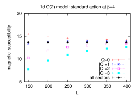
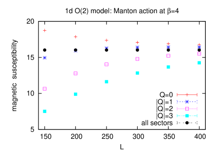
In analogy to Subsection 3.1, Figure 2 gives an overview over the values of $\chi_{{\rm m},|Q|}$ up to $|Q|=3$, at different $L$. Again we see that the value measured in all sectors is stable in $L$, whereas the topologically restricted results strongly depend on $L$ and $|Q|$. Hence the setting is suitable for the BCNW method also with respect to the magnetic susceptibility.

Figure 2: The magnetic susceptibility in the 1d O(2) model at $\beta=4$ on lattices of size $L=150\dots 400$, with the standard action (left) and the Manton action (right). We show $\chi_{\rm m}$ measured in all sectors (practically constant in this range of $L$), as well as $\chi_{{\rm m},|Q|}$ in the sectors $|Q|=0\dots 3$ (well distinct).

We proceed to the fits to search the optimal values — according to formula (2.4) — for the (over-determined) susceptibilities $\chi_{\rm m}$ and $\chi_{\rm t}$. Table 2 shows the results in the fitting ranges $L=L_{\rm min}\dots 400$, $L_{\rm min}=150,$ $250$, $300$, and $|Q|=0\dots|Q|_{\rm max}$, with $|Q|_{\rm max}=2$ or $3$.

		standard action		Manton action
$L_{\rm min}$	$|Q|_{\rm max}$	$\chi_{\rm m}$	$\chi_{\rm t}$	$\chi_{\rm m}$	$\chi_{\rm t}$
150	2	13.64(16)	0.0072(13)	16.11(35)	0.0054(18)
150	3	13.67(22)	0.0070(22)	16.14(41)	0.0050(26)
250	2	13.64(5)	0.0071(5)	16.00(14)	0.0060(8)
250	3	13.65(13)	0.0074(15)	15.99(28)	0.0064(20)
300	2	13.64(5)	0.0071(5)	16.02(12)	0.0058(8)
300	3	13.66(13)	0.0073(17)	16.02(29)	0.0061(23)
	all	13.6545(4)	0.007554	16.0187(5)	0.006333

Table 2: Results based on fits to formula (2.4), with input data for the magnetic susceptibility in the range $L=L_{\rm min}\dots 400$ and $|Q|\leq|Q|_{\rm max}$. The last line displays $\chi_{\rm m}$ measured in all sectors at $L=400$, and $\chi_{\rm t}$ at $L=\infty$.

The fitting results for both susceptibilities are compatible with the correct values, albeit the uncertainty of $\chi_{\rm t}$ is rather large. Without knowing the exact value one could combine the results of separate fits, which reduces the uncertainty, but it leads to a $\chi_{\rm t}$-value which is somewhat too small. On the other hand, for $\chi_{\rm m}$ the values are far more precise, and the relative uncertainty is on the percent level (or below) in each case. Here a combination which reduces the uncertainty is welcome, although it has to be done with care since the partial results are not independent of each other. We add that the fitting results for the coefficient $c$ are consistent with eq. (3.15), $c\simeq 1.6$, within (considerable) uncertainties.

The observed precisions for $\chi_{\rm m}$ and $\chi_{\rm t}$ can be understood if we consider the impact of the sub-leading contributions, which are missing in the BCNW formula (2.4): taking into account the additional terms up to the incomplete third order modifies the fitting results for $\chi_{\rm m}$ only on the permille level, but those for $\chi_{\rm t}$ in ${\cal O}(10)\,\%$, both with somewhat enhanced errors. Also a variety of further fitting variants, with the terms of a complete second or complete third order of approximation (3.14), with fixed or free additional terms, leads to consistent results for $\chi_{\rm m}$ and $\chi_{\rm t}$, but with enlarged errors. In summary, there seems to be no fitting strategy which improves the results compared to the simple 3-parameter fit based on the BCNW approximation (2.4).

4 Applications to the 2d Heisenberg model

Our study of the 2d Heisenberg model, or 2d O(3) model, uses quadratic lattices of unit spacing and square-shaped volumes $V=L\times L$. On each lattice site $x$ there is a classical spin $\vec{e}_{x}\in S^{2}$, and we implement periodic boundary conditions in both directions. We consider the standard lattice action as well as the constraint action [32],

$$S[\vec{e}\,]_{\rm standard} = \beta\sum_{x,\mu}(1-\vec{e}_{x}\cdot\vec{e}_{x+\hat{\mu}})\ ,$$

$$S[\vec{e}\,]_{\rm constraint} = \left\{\begin{array}[]{ccc}0&&\vec{e}_{x}\cdot\vec{e}_{x+\hat{\mu}}\geq\cos\delta\quad\forall x,\,\mu=1,2\\ +\infty&&{\rm otherwise,}\end{array}\right.$$ (4.3)

where $\delta$ is the constraint angle, and $\hat{\mu}$ is the unit vector in $\mu$-direction.

Our simulations were performed at $\beta=1.5$ and $\delta=0.55\,\pi$, respectively, with the correlation lengths

$${\rm standard~{}action}\ \ (L=84) : \xi=9.42(2)\ ,$$

$${\rm constraint~{}action}\ (L=96) : \xi=3.58(5)\ .$$ (4.4)

The cluster algorithm allowed us to perform ${\cal O}(10^{7})$ measurements at each lattice size shown in Figures 3 and 4.

For the topological charge we use again a geometric definition [2]. To this end, each plaquette is split into two triangles, in alternating orientation. We consider the oriented solid angle of the spins at the corners of a triangle: the sum of the two angles (divided by $4\pi$) within a plaquette (associated with the site $x$) amounts to its topological charge density $q_{x}$. Due to the periodic boundary conditions, their sum must be an integer, $Q=\sum_{x}q_{x}\in\mathbb{Z}$. Details and explicit formulae are given in Refs. [32, 22].

4.1 Action density

A study of the BCNW formula with respect to the action density (3.7) can only be performed with the standard action (in case of the constraint action all contributing configurations have action $S_{\rm constraint}=0$). Figure 3 shows the values of $s$ and $s_{|Q|}$, $|Q|\leq 2$ in the range $L=32\dots 84$. The total expectation value $s$ is stable within $0.0003$ for $L\geq 56$, while the topologically constrained results differ by ${\cal O}(10^{-3})$ even at $L=84$. Therefore $L=56\dots 84$ is a regime of moderate volumes, which is suitable for testing the BCNW formula.

Figure 3: The action density in the 2d O(3) model, on $L\times L$ lattices with the standard lattice action, in the sectors with topological charge $|Q|=0$, $1$, $2$, and summed over all sectors (i.e. all configurations used for the numerical measurements). The latter stabilizes to $0.3$ permille for $L\geq 56$.

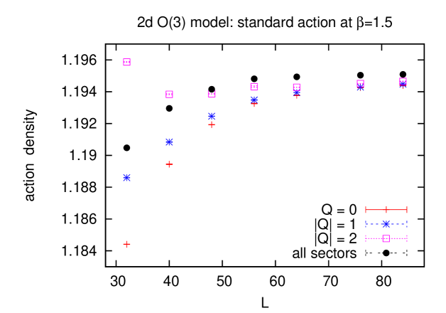
The fitting results, for $|Q|\leq 2$ and various ranges of $L$ are listed in Table 3. The fits do not match the BCNW formula perfectly, as expected, since the latter is an approximation, and the input data have very small statistical errors of ${\cal O}(10^{-5})$. Nevertheless, the value of $s$ is obtained correctly up to a high precision of $0.2$ permille. On the other hand, the determination of the topological susceptibility is less successful; only the fit with $L=76$ and $84$ yields a result, which is correct within the errors.

fitting range in $L$	$s$	$\chi_{\rm t}$	$\chi^{2}/$d.o.f.
56 — 64	1.1955(2)	0.0035(5)	2.66
56 — 76	1.19538(6)	0.0031(3)	2.66
56 — 84	1.19536(5)	0.0030(3)	2.63
64 — 76	1.19532(7)	0.0031(3)	2.65
64 — 84	1.19531(5)	0.0031(3)	2.58
76 — 84	1.1953(1)	0.0026(3)	2.60
$L=84$, all sectors	1.195089(5)	0.002323(3)

Table 3: Fitting results for the action density $s$ and the topological susceptibility $\chi_{\rm t}$ in the 2d O(3) model. The input data in fixed topological sectors are plotted in Figure 3.

4.2 Magnetic susceptibility and correlation length

We proceed to the constraint action (4.3) where our choice of $\delta$ yields a shorter correlation length, which favors the stabilization of observables (measured in all sectors) at smaller $L$. This can be seen in Figure 4, which shows the magnetic susceptibility $\chi_{\rm m}$, analogous to eq. (3.12) (again the disconnected part vanishes due to rotational symmetry), and the correlation length $\xi$. Stabilization within the errors is attained for $\chi_{\rm m}$ at $L\geq 48$ (with errors around $0.2$ permille), and for $\xi$ already at $L\geq 16$ (with errors of ${\cal O}(1)\,\%$). On the other hand, for $L=128$ the $\chi_{{\rm m},|Q|}$-values are not distinguished anymore from $\chi_{\rm m}$ beyond the errors, and the same happens for $\xi_{|Q|}$ already at $L=96$. Finally, we have to exclude $L=16$, because here we only obtain $\langle Q^{2}\rangle\simeq 0.63$, hence its inverse is not suitable as an expansion parameter. This singles out the regime of moderate volumes, where the BCNW formula is appropriate, to the range $L=48\dots 96$ for $\chi_{\rm m}$, and $L=32\dots 64$ for $\xi$.

Figure 4: Results for the magnetic susceptibility (above) and for the correlation length (below) in the 2d O(3) model, with the constraint action at $\delta=0.55\,\pi$. The windows, which are suitable for applications of the BCNW formula, are given by $L=48\dots 96$ for $\chi_{\rm m}$, and by $L=32\dots 64$ for $\xi$.

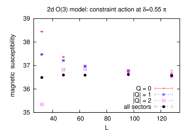
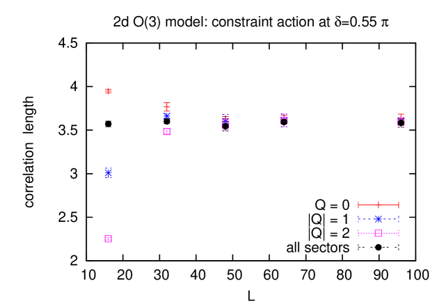
Our fitting results are given in Table 4. In the case of $\chi_{\rm m}$ we probe the BCNW formula (2.4) (with its incomplete second order, ${\cal O}(1/V^{2})$), as well as its extensions to the second order plus an incomplete third order as given in formula (2.2). For the latter option, the approximation is more precise, but an additional free parameter $\bar{c}$ hampers the fits.

	fitting	BCNW	incomplete	all sectors
	range	formula	3rd order	at $L_{\rm max}$
$\chi_{\rm m}$	48 — 64	36.56(4)	36.64(11)	36.590(9)
$\chi_{\rm t}$		0.0026(2)	0.0031(6)	0.0027935(14)
$\chi_{\rm m}$	48 — 96	36.58(3)	36.64(7)	36.616(9)
$\chi_{\rm t}$		0.0026(2)	0.0032(6)	0.0027942(11)
$\xi$	32 — 64	3.56(2)	3.58(4)	3.59(2)
$\chi_{\rm t}$		0.0027(3)	0.0034(14)	0.0027935(14)

Table 4: Fitting results based on data for $\chi_{\rm m}$ and for $\xi$ in the 2d O(3) model, in fitting ranges $L_{\rm min}$ — $L_{\rm max}$, and sectors with $|Q|\leq 2$. In the case of $\chi_{\rm m}$, with the optimal range, we show results for the BCNW approximation (2.4), as well as its extension to the complete second order plus one term of ${\cal O}(1/V^{3})$, according to formula (2.2).

For both fitting versions, the results for $\chi_{\rm m}$ and $\chi_{\rm t}$ are compatible with the directly measured values. We observe, however, that the inclusion of terms beyond the BCNW formula enhances the uncertainty (due to the additional fitting parameter). The uncertainty is on the permille level for $\chi_{\rm m}$, but large for $\chi_{\rm t}$, in particular with extra terms. (Without these terms it is around $8\,\%$.) It turns out to be non-profitable to extend the approximation beyond the BCNW formula.

The simple BCNW approximation is also superior for the fits with respect to $\xi$, where the additional terms drastically increase the uncertainty. The results in Table 4 are correct, within percent level for $\xi$, but again with a large uncertainty of the $\chi_{\rm t}$-value.

We add that we also tried fits to the complete second order approximation, without the third order term that appears in formula (2.2). However, this scenario (which also involves the fitting parameter $\bar{c}$) is clearly unfavorable: in this case, it often happens that the least-square fit even fails to converge to values in the correct magnitude.

To conclude, this study suggests that the simple BCNW formula, with only three free parameters, is in fact optimal for extracting values for the considered observable, and for $\chi_{\rm t}$. Moreover, we confirm that the method works best for the determination of the observable; it is less successful with respect to the determination of $\chi_{\rm t}$.

5 Results in 4d SU(2) Yang-Mills theory

The topological tunnelling rate has been investigated in 4d Yang-Mills theories with the heatbath [33] and the HMC algorithm [34]. In both cases the autocorrelation time with respect to $Q$ was found to increase drastically for decreasing lattice spacing, which further substantiates the motivation of our study.

5.1 Simulation setup

We consider 4d SU(2) Yang-Mills theory, which has the continuum action

$$S_{\rm cont}[A]=\beta_{\rm cont}\int d^{4}x\,F_{\mu\nu}^{a}(x)F_{\mu\nu}^{a}(x)\ ,$$ (5.1)

and the topological charge

$$Q[A]=\frac{1}{16\pi^{2}}\int d^{4}x\,\epsilon_{\mu\nu\rho\sigma}F_{\mu\nu}^{a}(x)F_{\rho\sigma}^{a}(x)\ .$$ (5.2)

On the lattice we simulate Wilson’s standard plaquette action. For the topological charge of a lattice gauge configuration $[U]$, we use an improved field-theoretic definition [3],

$$Q[U]=\frac{1}{16\pi^{2}}\sum_{x}\epsilon_{\mu\nu\rho\sigma}\sum_{\Box=1,2,3}\frac{c_{\Box}}{\Box^{4}}F_{x,\mu\nu}^{(\Box\times\Box)}[U]F_{x,\rho\sigma}^{(\Box\times\Box)}[U]\ ,$$ (5.3)

where $F_{x,\mu\nu}^{(\Box\times\Box)}[U]$ denotes the lattice field strength tensor, clover averaged over square-shaped loops of size $\Box\times\Box$, and $(c_{1},c_{2},c_{3})=(1.5,-0.6,0.1)$. Before applying eq. (5.3), we perform a number of cooling sweeps with the intention to remove local fluctuations in the gauge configurations, while preserving the topological structure.

Figure 5: Cooling and assignment of the topological charge for three typical gauge configurations, at $\beta=2.5$, in a lattice volume $V=18^{4}$.

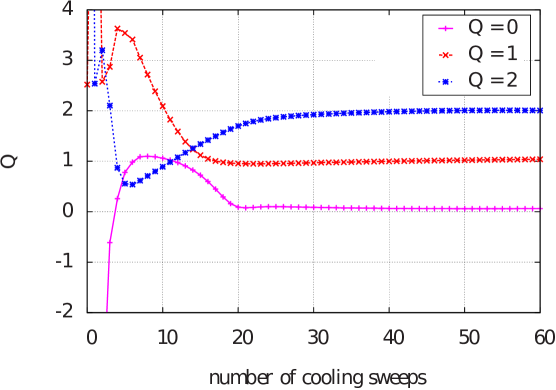
A cooling sweep amounts to a local minimization of the action, i.e. a minimization with respect to each gauge link within a short range. For this minimization we use again an improved lattice Yang-Mills action,

$$S[U]=\frac{\beta}{16}\sum_{x}\sum_{\mu\nu}\sum_{\Box=1,2,3}\frac{c_{\Box}}{\Box^{4}}\textrm{Tr}\Big{(}1\!\!1-W_{x,\mu\nu}^{(\Box\times\Box)}[U]\Big{)}\ ,$$ (5.4)

where $W_{x,\mu\nu}^{(\Box\times\Box)}[U]$ is a clover averaged loop of size $\Box\times\Box$ with the coefficients $c_{\Box}$ given above (for comparison, the standard plaquette action corresponds to $(c_{1},c_{2},c_{3})=(1,0,0)$). Choosing an appropriate number of cooling sweeps is a subtle and somewhat ambiguous task, which is carried out for each gauge configuration one by one. After every cooling sweep we compute $Q[U]$ according to eq. (5.3). As soon as $Q[U]$ is stable (it varies by less than 10 % and is close to an integer for at least 50 cooling sweeps), the corresponding close integer is the topological charge that we assign to the gauge configuration $[U]$. Figure 5 shows examples for typical cooling histories of gauge configurations with $Q=0$, $1$ and $2$. (Details of this procedure, and a comparison to other definitions of the topological charge, are discussed in Ref. [6].)

Our simulations were performed with a heatbath algorithm, see e.g. Ref. [35]. We set $\beta=2.5$, which corresponds to a lattice spacing $a\approx 0.073\,\textrm{fm}$, if the scale is set with the QCD Sommer parameter $r_{0}=0.46\,\textrm{fm}$ [36]. This value is in the range of lattice spacings $0.05\,\textrm{fm}\raisebox{-2.15277pt}{$\,\stackrel{{\scriptstyle<}}{{\scriptstyle\sim}}\,$}a\raisebox{-2.15277pt}{$\,\stackrel{{\scriptstyle<}}{{\scriptstyle\sim}}\,$}0.15\,\textrm{fm}$ typically used in contemporary QCD simulations. We generated gauge configurations in lattice volumes $V=L^{4}$, with $L=12,\,14,\,15,\,16,\,18$. In each volume, observables were measured on 4000 configurations, separated by 100 heatbath sweeps. This guarantees their statistical independence; in particular, even the auto-correlation time with respect to the topological charge $Q$ is below 20 heatbath sweeps.

5.2 Computation of observables

The observable we focus on is the static quark-antiquark potential ${\mathcal{V}}_{q\bar{q}}(r)$ for separations $r=1,2\ldots 6$. This quantity can be interpreted as the mass of a static-static meson. To determine ${\mathcal{V}}_{q\bar{q}}(r)$, we consider temporal correlation functions of operators

$$O_{q\bar{q}}(r)=\bar{q}(\vec{r}_{1})\,U^{\textrm{APE}}(\vec{r}_{1},\vec{r}_{2})\,q(\vec{r}_{2})\ ,\quad r=|\vec{r}_{1}-\vec{r}_{2}|\ ,$$ (5.5)

where $\bar{q}$, $q$ represent spinless static quarks, while $U^{\textrm{APE}}(\vec{r}_{1},\vec{r}_{2})$ denotes a product of APE smeared spatial links [37] along a straight line connecting the lattice sites $\vec{r}_{1}$ and $\vec{r}_{2}$ on a given time slice. For the quarks we use the HYP2 static action, which is designed to reduce UV fluctuations and, therefore, to improve the signal-to-noise ratio [38]. These temporal correlation functions can be simplified analytically resulting in Wilson loop averages $\langle W(r,t)\rangle$ with APE smeared spatial and HYP2 smeared temporal lines of length $r$ and $t$, respectively. Thus we arrive at the vacuum expectation value

$$\langle\Omega|O^{\dagger}_{\bar{q}q}(t)O_{\bar{q}q}(0)|\Omega\rangle\propto\Big{\langle}W(r,t)\Big{\rangle}\ .$$ (5.6)

We chose the APE smearing parameters as $N_{\textrm{APE}}=15$ and $\alpha_{\textrm{APE}}=0.5$, which (roughly) optimizes the overlap of $O_{\bar{q}q}|\Omega\rangle$ with the ground state of the static potential (for details of the smearing procedure we refer to Ref. [39], where a similar setup had been used).

5.3 Numerical results

5.3.1 The static potential

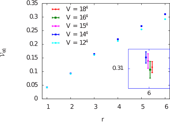
Figure 6 shows results for the static potential measured in all topological sectors, i.e. for each $r$ and $t$ the Wilson loop average is computed on all configurations, which are available in some volume. The volumes $14^{4}$, $15^{4}$, $16^{4}$ and $18^{4}$ yield identical results within statistical errors, but the static potential in the $12^{4}$ volume differs by several $\sigma$ for quark-antiquark separations $r\geq 3$. We conclude that $V=12^{4}$ entails sizable ordinary finite volume effects (not associated with topology fixing), whereas for volumes $V\geq 14^{4}$ such ordinary finite volume effects are negligible. Consequently, we do not use the $12^{4}$ lattice in the following fixed topology studies.

Figure 6: The static potential ${\mathcal{V}}_{q\bar{q}}(r)$ in a variety of lattice volumes $V=12^{4}\dots 18^{4}$.

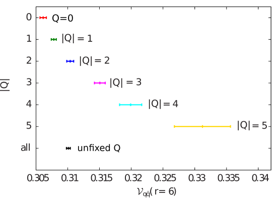
For $V=15^{4}$, Figure 7 demonstrates that static potentials obtained at fixed topology from different sectors $|Q|=0\ldots 5$ (by averaging only over configurations of a fixed charge $|Q|$), ${\mathcal{V}}_{q\bar{q},|Q|}$, differ significantly. For example ${\mathcal{V}}_{q\bar{q},0}(r=6)$ and ${\mathcal{V}}_{q\bar{q},4}(r=6)$ differ by more than $6\sigma$. They are also well distinct from the corresponding result in all sectors, ${\mathcal{V}}_{q\bar{q},|Q|\leq 1}(6)<{\mathcal{V}}_{q\bar{q}}(6)<{\mathcal{V}}_{q\bar{q},|Q|\geq 2}(6)$. These observations show that $V=14^{4}\dots 18^{4}$ is in the regime that we denoted as moderate volumes (cf. Section 2), where the BCNW method is appropriate to extract observables from fixed topology measurements. Similar results for the static potential in SU(3) Yang-Mills theory have been reported in Ref. [4].

Figure 7: The static potential at separation $r=6$, ${\mathcal{V}}_{q\bar{q}}(6)$, for fixed topological sectors $|Q|\leq 5$, and without topology fixing, in the volume $V=15^{4}$.

To extract the physical static potential from Wilson loop averages, separately computed in distinct topological sectors $|Q|\leq 7$ and some volume $V$, $\langle W_{V}(r,t)\rangle_{|Q|}$, we follow the procedure discussed in Ref. [15].

• We perform $\chi^{2}$ minimizing fits of either the $1/V$ expansion of the correlation function [14],

  $$C_{Q,V}(t)=\Big{\langle}W_{V}(r,t)\Big{\rangle}_{|Q|}$$

  $$\approx\alpha(r)\exp\bigg{\{}-\bigg{[}{\mathcal{V}}_{q\bar{q}}(r)+\frac{1}{2}{\mathcal{V}}^{\prime\prime}_{q\bar{q}}(r)\frac{1}{V\chi_{\rm t}}\bigg{(}1-\frac{Q^{2}}{V\chi_{\rm t}}\bigg{)}\bigg{]}t\bigg{\}}$$ (5.7)

  (cf. formula (2.4)), or of the improved approximation [16]

  $$C_{Q,V}(t)\simeq\frac{\alpha(r)}{\sqrt{1+{\mathcal{V}}^{\prime\prime}_{q\bar{q}}(r)t/(\chi_{\rm t}V)}}$$

  $$\hskip 19.20569pt\times\exp\bigg{(}-{\mathcal{V}}_{q\bar{q}}(r)t-\frac{1}{\chi_{\rm t}V}\bigg{(}\frac{1}{1+{\mathcal{V}}^{\prime\prime}_{q\bar{q}}(r)t/(\chi_{\rm t}V)}-1\bigg{)}\frac{1}{2}Q^{2}\bigg{)}\qquad\quad$$ (5.8)

  with respect to the parameters ${\mathcal{V}}_{q\bar{q}}(r)$, ${\mathcal{V}}^{\prime\prime}_{q\bar{q}}(r)=\partial^{2}_{\theta}{\mathcal{V}}_{q\bar{q}}(r,\theta)|_{\theta=0}$, $\alpha(r)$ ($r=1\ldots 6$) and $\chi_{\rm t}$ to the numerical results for $\langle W_{V}(r,t)\rangle_{|Q|}$ in the range $t_{\textrm{min}}\leq t\leq t_{\textrm{max}}$, where $t_{\textrm{min}}$ and $t_{\textrm{max}}$ are displayed in Table 5. When fitting formula (5.8), we also study the scenario where $\chi_{\rm t}$ is fixed to $\chi_{\rm t}=7\times 10^{-5}$, which was obtained in Ref. [3] by means of a direct measurement, in agreement with the fixed topology study in Ref. [22]. Moreover, we checked that the resulting fit parameters are stable within errors when we vary $t_{\textrm{min}}$ and $t_{\textrm{max}}$ by $\pm 1$.

  $V$	$t_{\textrm{min}}$	$t_{\textrm{max}}$	maximum $|Q|$ fulfilling	maximum $|Q|$ fulfilling
  			$1/(\chi_{\rm t}V),\,|Q|/(\chi_{\rm t}V)<1$	$1/(\chi_{\rm t}V),\,|Q|/(\chi_{\rm t}V)<0.5$
  $14^{4}$	5	7	2	1
  $15^{4}$	5	7	3	1
  $16^{4}$	5	8	4	2
  $18^{4}$	5	8	7	3

  Table 5: Temporal fitting ranges $t_{\textrm{min}}\ldots t_{\textrm{max}}$, and maximum topological charges $|Q|$, for the lattice volumes $V$ under consideration.

• The results for $\langle W_{V}(r,t)\rangle_{|Q|}$ entering the fit are restricted to those $|Q|$ and $V$ values for which $1/(\chi_{\rm t}V),\,|Q|/(\chi_{\rm t}V)<1$ or $<0.5$; we recall that the approximations (5.7) and (5.8) are only valid for sufficiently large $\chi_{\rm t}V=\langle Q^{2}\rangle$, and small $|Q|$. To implement this selection we insert $\chi_{\rm t}=7\times 10^{-5}$ [3]; Table 5 gives an overview.

• We either perform a single combined fit to all considered separations $r=1\ldots 6$, or six separate fits, one for each $r$. In the latter case we obtain six results for $\chi_{\rm t}$, which agree within the errors in most cases, cf. Subsection 5.3.2.

Table 6 collects the results for ${\mathcal{V}}_{q\bar{q}}(r)$ from fixed topology computations (using four volumes, $V=14^{4},\,15^{4},\,16^{4},\,18^{4}$), and computed in all sectors at $V=18^{4}$. There is agreement between most of these results within about $2\sigma$. Only for $r=1$, and the relaxed constraint $1/(\chi_{\rm t}V),\,|Q|/(\chi_{\rm t}V)<1$, there are a few cases with discrepancies beyond $3\sigma$, in particular for the expansion (5.7) (the corresponding data in Table 6 are displayed in italics).

The extent of the errors of the fitting results is fairly independent of the choice of the expansion ((5.7), or (5.8), or (5.8) with $\chi_{\rm t}=7\times 10^{-5}$ fixed). The errors increase, however, by factors up to $\approx 2$, when we implement the stringent constraint $1/(\chi_{\rm t}V),\,|Q|/(\chi_{\rm t}V)<0.5$, which is expected, since less input data are involved, see Table 5. All fits of the expansions (5.7) and (5.8) capture well the fixed topology results.

method	$\mathcal{V}_{q\bar{q}}(1)$	$\mathcal{V}_{q\bar{q}}(2)$	$\mathcal{V}_{q\bar{q}}(3)$	$\mathcal{V}_{q\bar{q}}(4)$	$\mathcal{V}_{q\bar{q}}(5)$	$\mathcal{V}_{q\bar{q}}(6)$
all sectors,    $V=18^{4}$
	0.04229(1)	0.09329(2)	0.1646(1)	0.2190(1)	0.2664(2)	0.3101(3)
fixed topology,    $V\in\{14^{4},\,15^{4},\,16^{4},\,18^{4}\}$,    $1/(\chi_{\rm t}V),\,|Q|/(\chi_{\rm t}V)<1$
(5.7)c	0.04240(3)	0.09343(8)	0.1646(2)	0.2189(3)	0.2662(4)	0.3097(5)
(5.7)s	0.04241(3)	0.09342(9)	0.1646(2)	0.2189(3)	0.2662(4)	0.3097(6)
(5.8)c	0.04230(3)	0.09324(8)	0.1644(2)	0.2187(3)	0.2661(4)	0.3098(6)
(5.8)s	0.04240(3)	0.09338(9)	0.1645(2)	0.2188(3)	0.2661(4)	0.3098(6)
(5.8)c$\chi_{\rm t}$	0.04225(3)	0.09326(8)	0.1643(2)	0.2186(3)	0.2660(4)	0.3097(6)
(5.8)s$\chi_{\rm t}$	0.04225(3)	0.09326(8)	0.1643(2)	0.2186(3)	0.2660(4)	0.3097(6)
fixed topology,    $V\in\{14^{4},\,15^{4},\,16^{4},\,18^{4}\}$,    $1/(\chi_{\rm t}V),\,|Q|/(\chi_{\rm t}V)<0.5$
(5.7)c	0.04227(4)	0.09326(14)	0.1645(3)	0.2190(5)	0.2665(7)	0.3103(10)
(5.7)s	0.04226(4)	0.09322(13)	0.1644(3)	0.2189(5)	0.2666(8)	0.3105(11)
(5.8)c	0.04227(4)	0.09326(14)	0.1645(4)	0.2190(5)	0.2665(7)	0.3104(10)
(5.8)s	0.04226(4)	0.09323(13)	0.1645(3)	0.2189(5)	0.2665(8)	0.3104(10)
(5.8)c$\chi_{\rm t}$	0.04225(4)	0.09317(12)	0.1643(3)	0.2186(4)	0.2660(6)	0.3096(8)
(5.8)s$\chi_{\rm t}$	0.04225(3)	0.09317(12)	0.1643(3)	0.2186(4)	0.2660(6)	0.3096(8)

Table 6: Results for the static potential ${\mathcal{V}}_{q\bar{q}}(r)$ for separations $r=1\ldots 6$ measured with and without topology fixing. In the column “method” the equation number of the expansion is listed, “c” denotes a single combined fit for all separations $r=1\ldots 6$, “s” denotes a separate fit for each separation, and $\chi_{\rm t}$ indicates that the topological susceptibility is not a fit parameter, but fixed to $\chi_{\rm t}=7\times 10^{-5}$. Fixed topology results, which differ by more than $3\sigma$ from the directly computed value, are written in italics.

For the extraction of the potential it seems essentially irrelevant whether a single combined fit or six separate fits are performed. Both the mean values and the statistical errors of ${\mathcal{V}}_{q\bar{q}}(r)$ are in most cases very similar. A single combined fit, however, seems somewhat advantageous regarding the determination of $\chi_{\rm t}$, see Subsection 5.3.2.

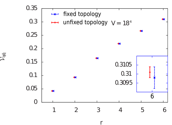
Figure 8 compares the static potential obtained from fixed topology Wilson loops, and computed without topology fixing at $V=18^{4}$. As reflected by Table 6 there is excellent agreement within the errors.

Figure 8: Comparison of static potential obtained from fixed topology Wilson loops, in the volumes $V=14^{4},\,15^{4},\,16^{4},\,18^{4}$, with $1/(\chi_{\rm t}V),\,|Q|/(\chi_{\rm t}V)<1$, using expansion (5.8) with one combined fit, and directly measured at $V=18^{4}$. (Since unfixed and fixed topology results coincide within the errors, they are shifted horizontally for better visibility.)

The expansion (5.7) of fixed topology Wilson loop averages $\langle W_{V}(r,t)\rangle_{|Q|}$ is a decaying exponential in $t$. This suggests defining a static potential at fixed topological charge $|Q|$ and volume $V$,

$$\mathcal{V}_{q\bar{q},|Q|,V}(r)=-\frac{d}{dt}\ln\Big{(}\Big{\langle}W_{V}(r,t)\Big{\rangle}_{|Q|}\Big{)}$$ (5.9)

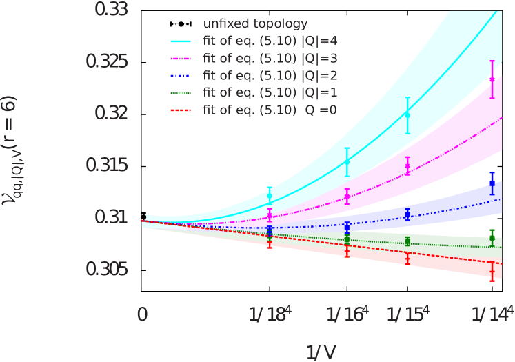
for some value of $t$, where formula (5.7) is a rather precise approximation. Within statistical errors $\mathcal{V}_{q\bar{q},|Q|,V}(r)$ is independent of $t$ for $t_{\textrm{min}}\leq t\leq t_{\textrm{max}}$. Therefore, we determine $\mathcal{V}_{q\bar{q},|Q|,V}(r)$ by a $\chi^{2}$ minimizing fit of a constant to the right-hand-side of eq. (5.9), with the derivative replaced by a finite difference (this is the common definition of an effective mass) in the interval $t_{\textrm{min}}\leq t\leq t_{\textrm{max}}$. For $|Q|=0\ldots 4$ and $V=14^{4},15^{4},16^{4},18^{4}$, the values for $\mathcal{V}_{q\bar{q},|Q|,V}(r=6)$ are plotted in Figure 9. As already shown in Figure 7, there is a strong dependence on the topological sector, which becomes increasingly prominent for smaller volumes. From expansion (5.7) the fixed topology static potential is expected to behave as

$$\mathcal{V}_{q\bar{q},|Q|,V}(r)\approx{\mathcal{V}}_{q\bar{q}}(r)+\frac{1}{2}{\mathcal{V}}^{\prime\prime}_{q\bar{q}}(r)\frac{1}{V\chi_{\rm t}}\bigg{(}1-\frac{Q^{2}}{V\chi_{\rm t}}\bigg{)}\ .$$ (5.10)

The corresponding curves for $|Q|=0\ldots 4$, with parameters ${\mathcal{V}}_{q\bar{q}}(r=6)$, ${\mathcal{V}}^{\prime\prime}_{q\bar{q}}(r=6)$ and $\chi_{\rm t}$ determined by the previously discussed fits ($V=14^{4}\dots 18^{4}$, $1/(\chi_{\rm t}V)$,$\,|Q|/(\chi_{\rm t}V)<1$, expansion (5.7) and a single combined fit), are also shown in Figure 9. One clearly sees that approximation (5.10) nicely describes the numerical results for $\mathcal{V}_{q\bar{q},|Q|,V}(r=6)$.

Figure 9: The fixed topology static potential $\mathcal{V}_{q\bar{q},Q,V}(r=6)$ for $|Q|=0\ldots 4$, as a function of $1/V$, and the curves corresponding to approximation (5.10).

We conclude that one can obtain a correct and accurate physical static potential from Wilson loops separately computed in different topological sectors. The errors are larger by factors $\approx 2\ldots 5$ (cf. Table 6) for a fixed topology computation using four ensembles, compared to a corresponding direct computation using a single ensemble ($V=18^{4}$).

5.3.2 The topological susceptibility

In Table 7 we present results for the topological susceptibility extracted from fixed topology Wilson loops $\langle W_{V}(r,t)\rangle_{|Q|}$. Again we use the $1/V$ expansion (5.7) or (5.8), the constraints $1/(\chi_{\rm t}V),\,|Q|/(\chi_{\rm t}V)<1$ or $<0.5$, and either a single combined fit to all considered separations $r=1\ldots 6$, or six separate fits, one for each $r$. The latter yields six different results for $\chi_{\rm t}$.

method	$\mathcal{V}_{q\bar{q}}(1)$	$\mathcal{V}_{q\bar{q}}(2)$	$\mathcal{V}_{q\bar{q}}(3)$	$\mathcal{V}_{q\bar{q}}(4)$	$\mathcal{V}_{q\bar{q}}(5)$	$\mathcal{V}_{q\bar{q}}(6)$
fixed topology,    $V\in\{14^{4},\,15^{4},\,16^{4},\,18^{4}\}$,    $1/(\chi_{\rm t}V),\,|Q|/(\chi_{\rm t}V)<1$
(5.7)c	8.8(0.5)
(5.7)s	8.8(0.5)	8.7(0.6)	8.6(0.7)	8.6(0.9)	8.8(1.0)	8.9(1.2)
(5.8)c	7.1(0.6)
(5.8)s	8.6(0.5)	8.2(0.7)	7.7(0.8)	7.3(0.9)	7.0(1.0)	6.7(1.1)
fixed topology,    $V\in\{14^{4}\,,\,15^{4}\,,\,16^{4}\,,\,18^{4}\}$,    $1/(\chi_{\rm t}V),\,|Q|/(\chi_{\rm t}V)<0.5$
(5.7)c	11.8(5.9)
(5.7)s	10.0(14.0)	20.7(44.3)	11.1(8.2)0	11.8(16.0)	12.8(8.7)0	15.4(52.1)
(5.8)c	11.9(5.4)
(5.8)s	10.2(21.8)	10.7(12.5)	11.3(8.7)0	11.8(5.8)0	13.0(9.7)0	14.6(12.2)

Table 7: Results for the topological susceptibility $\chi_{\rm t}\times 10^{5}$ from fixed topology computations of the static potential ${\mathcal{V}}_{q\bar{q}}(r)$ for various separations $r=1\ldots 6$. In the column “method” the equation number of the expansion is listed, “c” denotes a single combined fit for all separations $r=1\ldots 6$, and “s” denotes a separate fit for each separation. The reference value from a direct computation is $\chi_{\rm t}\times 10^{5}=(7.0\pm 0.9)$ [3].

Not all of the extracted $\chi_{\rm t}$ values perfectly agree with each other or with the result $\chi_{\rm t}=(7.0\pm 0.9)\times 10^{-5}$ from Ref. [3], which we take as a reference. Using the weak constraint $1/(\chi_{\rm t}V),\,|Q|/(\chi_{\rm t}V)<1$ there seems to be a slight tension in form of $\approx 2\sigma$ discrepancies, when performing fits with formula (5.7). The extended expansion (5.8) gives somewhat better results: no tension shows up, and most results agree with the reference value within $\sigma$.

One might hope for further improvement by using the stronger constraint $1/(\chi_{\rm t}V),\,|Q|/(\chi_{\rm t}V)<0.5$, since then formulae (5.7) and (5.8) are more accurate. Indeed this leads to consistency with the reference value, but in most cases the errors are very large, of the order of 100 % or even more. For this strong constraint the available ${\mathcal{V}}_{q\bar{q},|Q|}$-data are not sufficient to extract a useful result for $\chi_{\rm t}$. Note that here the error for one combined fit is significantly smaller than those for the separate fits.

We conclude that — in principle — one can extract the topological susceptibility in Yang-Mills theory from the static potential at fixed topology using formulae like (5.7) or (5.8). In practice, however, one needs precise data in several large volumes. Only when a variation of the input data (e.g. by using different bounds with respect to $1/(\chi_{\rm t}V),\,|Q|/(\chi_{\rm t}V)$) leads to precise and stable $\chi_{\rm t}$ values, should one consider the result trustworthy. The data used in this work are not sufficient to achieve this standard. As we mentioned before, more promising methods to determine $\chi_{\rm t}$ from simulations at fixed topology using the same lattice setup have recently been explored [22, 23, 24, 26].

6 Results in the Schwinger model

6.1 Simulation setup

We finally proceed to the Schwinger model — or 2d Quantum Electrodynamics — as a test model with dynamical fermions. This model has the continuum Lagrangian

$$\mathcal{L}_{\rm cont}(\psi,\bar{\psi},A)=\sum_{{\rm f}=1}^{N_{\rm f}}\bar{\psi}^{\rm(f)}\Big{(}\gamma_{\mu}(\partial_{\mu}+{\rm i}g_{\rm cont}A_{\mu})+m^{\rm(f)}\Big{)}\psi^{\rm(f)}+\frac{1}{4}F_{\mu\nu}F_{\mu\nu}\ ,$$ (6.1)

where $N_{\rm f}$ is the number of fermion flavors. It is a widely used toy model, which shares important features with QCD. In particular the U(1) gauge theory in two (spacetime) dimensions allows for topologically non-trivial gauge configurations, similar to instantons in 4d Yang-Mills theories and in QCD. The topological charge is given by

$$Q[A]=\frac{1}{\pi}\int d^{2}x\,\epsilon_{\mu\nu}F_{\mu\nu}\ .$$ (6.2)

Moreover, for $N_{\rm f}=2$ the low lying energy eigenstates contain a light iso-triplet composed of quasi Nambu-Goldstone bosons, which we are going to denote as “pions”. This model also exhibits fermion confinement.

We simulated the Schwinger model on periodic lattices of volume $V=L\times L$ (as before we use lattice units), with $N_{\rm f}=2$ mass degenerate flavors. They are represented by Wilson fermions, and we use the standard plaquette gauge action (see e.g. Ref. [40]).

One can approach the continuum limit by increasing $L$, while keeping the terms $gL$ and $M_{\pi}L$ fixed, where $M_{\pi}$ denotes the pion mass. This requires decreasing both $g$ and $M_{\pi}$ proportional to $1/L$ (for the latter the fermion mass has to be adjusted). It is also common to refer to $\beta=1/g^{2}$, in analogy to the previous sections.

As in Sections 3 and 4, we employ a geometric definition of the topological charge on the lattice [41],

$$Q[U]=\frac{1}{2\pi}\sum_{P}\phi(P)\ ,$$ (6.3)

where $\sum_{P}$ denotes the sum over all plaquettes $P=e^{{\rm i}\phi(P)}$, $-\pi<\phi(P)\leq\pi$. With this definition, $Q\in\mathbb{Z}$ holds for any stochastic gauge configuration.

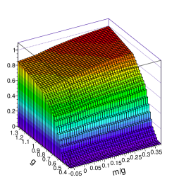
We performed simulations at various values of $\beta$, $m$ and $L$ using the HMC algorithm of Ref. [42], with multiple timescale integration and mass preconditioning [43]. We started with rather short simulations ($\approx 50\,000\ldots 100\,000$ HMC trajectories) on small lattices ($L=8\ldots 28$), to investigate the transition probability between topological sectors per HMC trajectory. This probability is plotted in Figure 10, as a function of $g=1/\sqrt{\beta}$ and $m/g$, while $gL=24/\sqrt{5}$ is kept constant. (The ratio $m/g$ is proportional to the bare fermion mass in physical units.) As expected, topological transitions are frequent at large couplings $g$ (coarse lattices), whereas at weak coupling (fine lattices) topology freezing is observed. Such a freezing is also observed in QCD, which is the main motivation of this work. We see that the dependence of the transition probability on the ratio $m/g$, and therefore on the dimensional bare fermion mass, is rather weak.

Figure 10: The transition probability to a different topological sector per HMC trajectory as a function of $g=1/\sqrt{\beta}$ (varying the lattice spacing in physical units, $a\propto g$) and $m/g$ (varying the bare fermion mass in physical units) at $gL=24/\sqrt{5}$ (fixed dimensional volume and coupling constant).

Similarly to the previous two sections we now explore the possibility of extracting physical energy levels (the “hadron” masses in the Schwinger model) from simulations at fixed topology. To obtain such results with small statistical errors, we focused on a single coupling and a single “quark” mass,

$$\beta=4\ ,\quad m=0.1\ ,$$ (6.4)

and we performed long simulations ($\approx 500\,000$ HMC trajectories) for volumes $V=L\times L$, with $L=40,\,44\,,48\,,52\,,56\,,60$.

6.2 Computation of observables

We determine the topological charge $Q[U]$ for each gauge configuration $U$ according to definition (6.3). (To measure observables at fixed topological charge $\nu$, we only use the configurations with $Q[U]=\nu$.)

The hadron masses that we investigate are the static potential $\mathcal{V}_{\bar{q}q}(r)$, which has been discussed before in Yang-Mills theory (Subsection 5.2), and the pion mass $M_{\pi}$. A suitable pion creation operator reads

$$O_{\pi}=\sum_{x}\bar{\psi}^{(u)}_{x}\gamma_{3}\psi^{(d)}_{x}\ ,$$ (6.5)

where $u$ and $d$ label the two (degenerate) fermion flavors. For the static potential we use again

$$O_{q\bar{q}}=\bar{q}(r_{1})U(r_{1};r_{2})q(r_{2})\ ,\quad r=|r_{1}-r_{2}|\ .$$ (6.6)

Also here $\bar{q}$ and $q$ represent spinless static fermions and $U(r_{1};r_{2})$ denotes the product of spatial links connecting the lattice sites $r_{1}$ and $r_{2}$ on a given time slice. Since there is only one spatial dimension, we do not apply any gauge link smearing.

6.3 Numerical results

6.3.1 The pion mass and the static potential

Similar to eq. (5.9) one can define a pion mass at fixed topological charge $|Q|$ and volume $V$ by

$$M_{\pi,|Q|,V}=-\frac{d}{dt}\ln\Big{(}\Big{\langle}O_{\pi}^{\dagger}(t)O_{\pi}(0)\Big{\rangle}\Big{)}$$ (6.7)

for some value of $t$, where approximation (5.7) is quite precise. Within statistical errors, $M_{\pi,|Q|,V}$ is independent of $t$ for large $t$. Therefore, we determine $M_{\pi,|Q|,V}$ by a $\chi^{2}$ minimizing fit of a constant to the right-hand-side of eq. (6.7) (with the derivative replaced by a finite difference).

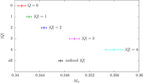
Figure 11 shows that pion masses obtained at fixed topology in different topological sectors, $M_{\pi,|Q|}$, differ significantly at $V=40^{2}$. For example $M_{\pi,0}$ and $M_{\pi,3}$ differ by more than $6\sigma$. The physically meaningful value measured in all sectors, $M_{\pi}$, also deviates e.g. from $M_{\pi,0}$ by more than $7\sigma$. Figure 11 demonstrates also here the necessity to analytically assemble fixed topology results, when the Monte Carlo algorithm is unable to generate frequent changes in $Q$.

Figure 11: The pion masses $M_{\pi,|Q|}$ in distinct topological sectors $|Q|=0\ldots 4$, and $M_{\pi}$ obtained in all sectors, in the volume $V=40^{2}$.

To determine the pion mass and the static potential from correlation functions evaluated in single topological sectors, $M_{\pi,|Q|}$ and ${\cal V}_{q\bar{q},|Q|}$, we follow the lines of Section 5. We perform least-square fits using expansion (5.7) or (5.8) of the correlation functions. We choose a suitable fitting range $t_{\textrm{min}}\ldots t_{\textrm{max}}$, which typically leads to $\chi^{2}/\textrm{d.o.f.}\raisebox{-2.15277pt}{$\,\stackrel{{\scriptstyle<}}{{\scriptstyle\sim}}\,$}1$. The stability of the resulting $M_{\pi,|Q|}$ and ${\cal V}_{q\bar{q},|Q|}$ has been checked by varying $t_{\textrm{min}}$ and $t_{\textrm{max}}$ by $\pm 1$. The $t$ ranges used for the determination of the pion mass are listed in Table 8.

$V$	$t_{\textrm{min}}$	$t_{\textrm{max}}$	maximum $|Q|$ for	maximum $|Q|$ for
			$1/(\chi_{\rm t}V)$, $|Q|/(\chi_{\rm t}V)<1$	$1/(\chi_{\rm t}V)$, $|Q|/(\chi_{\rm t}V)<0.5$
$40^{2}$	$12$	$16$	$7$	$3$
$44^{2}$	$12$	$18$	$9$	$4$
$48^{2}$	$12$	$20$	$11$	$5$
$52^{2}$	$12$	$22$	$13$	$6$
$56^{2}$	$12$	$24$	$15$	$7$
$60^{2}$	$12$	$24$	$17$	$8$

Table 8: Temporal fitting ranges $t_{\textrm{min}}\ldots t_{\textrm{max}}$ and maximum topological charges $|Q|$ for the volumes $V$ under consideration.

We perform fits in three different ways: (“c”) a single combined fit to all five observables ($M_{\pi}$, $\mathcal{V}_{q\bar{q}}(r=1)$, $\mathcal{V}_{q\bar{q}}(r=2)$, $\mathcal{V}_{q\bar{q}}(r=3)$, $\mathcal{V}_{q\bar{q}}(r=4)$); (“c$\mathcal{V}$”) a single combined fit to the four static potential observables; (“s”) five separate fits, one to each of the five observables. The results are collected in Table 9, along with reference values obtained in all sectors at $V=60^{2}$.

The conclusions are essentially the same as for Yang-Mills theory discussed in Section 5. Results extracted indirectly, from simulations at fixed topology, are in agreement with those obtained directly. The magnitude of the errors is the same for the two expansions (5.7) and (5.8), and for the fitting methods “c”, “c$\mathcal{V}$” and “s”. They are, however, larger by factors of $\approx 2$ when we use the stringent constraint $1/(\chi_{\rm t}V),\,|Q|/(\chi_{\rm t}V)<0.5$, since less input data are involved compared to $1/(\chi_{\rm t}V),\,|Q|/(\chi_{\rm t}V)<1$. The fits all yield uncorrelated $\chi^{2}/\textrm{d.o.f.}\raisebox{-2.15277pt}{$\,\stackrel{{\scriptstyle<}}{{\scriptstyle\sim}}\,$}1$, indicating that the fixed topology results are well described by both formulae (5.7) and (5.8).

method	$M_{\pi}$	$\mathcal{V}_{q\bar{q}}(1)$	$\mathcal{V}_{q\bar{q}}(2)$	$\mathcal{V}_{q\bar{q}}(3)$	$\mathcal{V}_{q\bar{q}}(4)$
all sectors,    $V=60^{2}$
	0.3474(3)	0.1296(2)	0.2382(5)	0.3288(7)	0.4045(10)
fixed topology,  $V\in\{40^{2},44^{2},48^{2},52^{2},56^{2},60^{2}\}$,  $1/(\chi_{\rm t}V)$, $|Q|/(\chi_{\rm t}V)<1$
(5.7)c	0.3466(16)	0.1293(19)	0.2370(23)	0.3261(29)	0.4022(62)
(5.7)c$\mathcal{V}$		0.1295(10)	0.2372(12)	0.3386(15)	0.4052(16)
(5.7)s	0.3477(8)   ​​​	0.1285(7)   ​​​	0.2371(9)   ​​​	0.3282(12)	0.4050(16)
(5.8)c	0.3467(10)	0.1293(6)   ​​​	0.2377(9)   ​​​	0.3321(32)	0.4059(69)
(5.8)c$\mathcal{V}$		0.1295(5)   ​​​	0.2379(11)	0.3392(14)	0.4049(16)
(5.8)s	0.3477(9)   ​​​	0.1294(5)   ​​​	0.2374(6)   ​​​	0.3288(12)	0.4040(15)
fixed topology,  $V\in\{40^{2},44^{2},48^{2},52^{2},56^{2},60^{2}\}$,  $1/(\chi_{\rm t}V)$, $|Q|/(\chi_{\rm t}V)<0.5$
(5.7)c	0.3454(32)	0.1284(27)	0.2364(28)	0.3311(50)	0.4049(80)
(5.7)c$\mathcal{V}$		0.1282(12)	0.2370(16)	0.3312(35)	0.4175(82)
(5.7)s	0.3478(32)	0.1292(12)	0.2377(21)	0.3275(61)	0.4027(91)
(5.8)c	0.3455(32)	0.1285(16)	0.2365(19)	0.3310(49)	0.4048(78)
(5.8)c$\mathcal{V}$		0.1287(9)   ​​​	0.2371(23)	0.3312(36)	0.4073(83)
(5.8)s	0.3482(35)	0.1291(11)	0.2376(13)	0.3290(22)	0.4036(55)

Table 9: Results for the pion mass $M_{\pi}$ and the static potential ${\mathcal{V}}_{q\bar{q}}(r)$ at separations $r=1,2,3,4$, with and without topology fixing. In the column “method” the equation number of the expansion is listed, “c” denotes one combined fit to all five observables, “c$\mathcal{V}$” means one combined fit to the four static potential observables, and “s” indicates separate fits for each of the five observables.

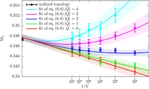
For $|Q|=0\ldots 4$ and $V=40^{2}\dots 60^{2}$, the $M_{\pi,|Q|,V}$ values are plotted in Figure 12. Again we observe a strong dependence on the topological sector, in particular in small volumes. From the expansion (5.7), $M_{\pi,|Q|,V}$ is expected to behave as approximation (2.4),

$$M_{\pi,Q,V}=M_{\pi}+\frac{c}{V\chi_{\rm t}}\bigg{(}1-\frac{Q^{2}}{V\chi_{\rm t}}\bigg{)}\ ,\quad c=\frac{1}{2}M_{\pi}^{\prime\prime}(\theta)_{\pi}|_{\theta=0}\ .$$ (6.8)

The corresponding curves for $|Q|=0\ldots 4$ with parameters $M_{\pi}$, $M^{\prime\prime}_{\pi}$ and $\chi_{\rm t}$, determined by the previously discussed fit “(5.7)s”, are also shown in Figure 12. One can clearly see that approximation (6.8) nicely captures the lattice results for $M_{\pi,|Q|,V}$.

Figure 12: The fixed topology pion mass $M_{\pi,|Q|,V}$ for $|Q|=0\dots 4$, as a function of $1/V$, and the curves corresponding to formula (6.8).

We conclude, similar to our study in Yang-Mills theory, that it is possible to extract correct and accurate values for the pion mass and the static potential from correlation functions computed in a number of fixed topological sectors and volumes. The errors are somewhat larger than for direct computation, in our case by factors of $\approx 2\ldots 7$. This is partly due to the smaller amount of gauge configurations of the fixed $Q$ ensembles at different $V$, and partly due to the extrapolation to infinite volume.

6.3.2 The topological susceptibility

Table 10 presents results for the topological susceptibility extracted from our data for $M_{\pi,|Q|}$ and ${\cal V}_{q\bar{q},|Q|}$. These values for $\chi_{\rm t}$ are obtained from the same fits, which lead to the results in Table 9. The results for $\chi_{\rm t}$ and their interpretation are similar to those obtained in Yang-Mills theory. We observe a slight tension of $\approx 2\sigma$ for some values, when using expansion (5.7) and the relaxed constraint ($1/(\chi_{\rm t}V),|Q|/(\chi_{\rm t}V)<1$). This tension disappears when we apply the improved expansion (5.8). When imposing the strict constraint ($1/\chi_{\rm t}V,\,|Q|/\chi_{\rm t}V<0.5$), we encounter the same problem as in Subsection 5.3.2: all results are in agreement with the directly measured $\chi_{\rm t}=\langle Q^{2}\rangle/V$ (at $V=60^{2}$), but the errors are very large.

method	$M_{\pi}$	$\mathcal{V}_{q\bar{q}}(1)$	$\mathcal{V}_{q\bar{q}}(2)$	$\mathcal{V}_{q\bar{q}}(3)$	$\mathcal{V}_{q\bar{q}}(4)$
all sectors,     $V=60^{2}$
0.0048(1)
fixed topology,  $V\in\{40^{2},44^{2},48^{2},52^{2},56^{2},60^{2}\}$,  $1/(\chi_{\rm t}V)$, $|Q|/(\chi_{t}V)<1$
(5.7)c	0.0038(5)
(5.7)c$\mathcal{V}$		0.0042(5)
(5.7)s	0.0041(4)	0.0038(5)	0.0036(7)	0.0038(11)	0.0044(9)
(5.8)c	0.0044(4)
(5.8)c$\mathcal{V}$		0.0042(6)
(5.8)s	0.0046(5)	0.0043(4)	0.0045(7)	0.0036(12)	0.0038(8)
fixed topology,  $V\in\{40^{2},44^{2},48^{2},52^{2},56^{2},60^{2}\}$,  $1/(\chi_{\rm t}V)$, $|Q|/(\chi_{\rm t}V)<0.5$
(5.7)c	0.0065(35)
(5.7)c$\mathcal{V}$		0.0017(30)
(5.7)s	0.0014(38)	0.0049(32)	0.0057(31)	0.0037(48)	0.0032(27)
(5.8)c	0.0067(32)
(5.8)c$\mathcal{V}$		0.0018(33)
(5.8)s	0.0017(32)	0.0043(34)	0.0022(46)	0.0015(38)	0.0048(52)

Table 10: Results for the topological susceptibility $\chi_{\rm t}$, directly measured (at $V=60^{2}$), and based on fixed topology computations of $M_{\pi,|Q|}$ and $\mathcal{V}_{q\bar{q},|Q|}(r)$ for separations $r=1,2,3,4$. In the column “method” the equation number of the expansion is listed, “c” denotes a single combined fit to all five observables, “c$\mathcal{V}$” means a single combined fit to the four static potential observables, and “s” denotes a separate fit to each of the five observables.

We infer that a reasonably accurate determination of the topological susceptibility from $M_{\pi,|Q|}$ and $\mathcal{V}_{q\bar{q},|Q|}$ requires extremely precise input data. The fixed topology ensembles and correlation functions of this work are not sufficient to extract an accurate and stable value for $\chi_{\rm t}$.

7 Conclusions

We have systematically explored the applicability of the Brower-Chandrasekharan-Negele-Wiese (BCNW) method [14] with lattice data in fixed topological sectors. Our study encompasses the quantum rotor, the Heisenberg model, 4d SU(2) Yang-Mills theory and the 2-flavor Schwinger model. The originally suggested application to the pion mass has been extended to other observables, like the magnetic susceptibility and the static quark-antiquark potential.

The primary goal of this method is the determination of a physical observable if only fixed topology results are available. Our observations show that this can be achieved to a good precision with input data from various volumes and topological sectors, which obey the (rather relaxed) constraint $1/(\chi_{\rm t}V),\,|Q|/(\chi_{\rm t}V)<1$. Hence this method is promising for application in QCD, where lattice spacings below $a\simeq 0.05\ {\rm fm}$ are expected to confine HMC simulations to a single topological sector over extremely long trajectories.

As a second goal, this method also enables — in principle — the determination of the topological susceptibility $\chi_{\rm t}$. In our study we obtained the right magnitude also for $\chi_{\rm t}$, but the results were usually plagued by large uncertainties. For this purpose, i.e. for the measurement of $\chi_{\rm t}$ based on fixed topology simulation results, other methods are more appropriate, based on the topological charge density correlation [21, 23, 22], or on an analysis of $\chi_{\rm t}$ in sub-volumes [24, 26].

Regarding the optimal way to apply this method, it seems — for lattice data of typical statistical precision — not really helpful to add additional terms of the $1/(\chi_{\rm t}V)$ expansion, beyond the incomplete second order that was suggested in Ref. [14]. Higher terms were elaborated in Ref. [16], and they improve the agreement with the fixed topology lattice data, but due to the appearance of additional free parameters they hardly improve the results for the physical observable and for $\chi_{\rm t}$.

A step beyond, which deserves being explored in more detail, is the inclusion of ordinary finite size effects (not related to topology fixing) [18], which even allows for the use of small volumes (in the terminology of Section 2).

At this point, we recommend the application of the simple formulae (2.4) and (5.7) or (slightly better) (5.8), with only three free parameters, for the determination of hadron masses in QCD on fine lattices, in particular in the presence of very light quarks.

Acknowledgements  We thank Irais Bautista and Lilian Prado for their contributions to this project at an early stage, and Carsten Urbach for providing a simulation code for the Schwinger model, corresponding advice and helpful discussions. This work was supported by the Helmholtz International Center for FAIR within the framework of the LOEWE program launched by the State of Hesse, and by the Mexican Consejo Nacional de Ciencia y Tecnología (CONACYT) through projects CB-2010/155905 and CB-2013/222812, as well as DGAPA-UNAM, grant IN107915. A.D., C.C. and M.W. acknowledge support by the Emmy Noether Programme of the DFG (German Research Foundation), grant WA 3000/1-1, and C.P.H. was supported through the project Redes Temáticas de Colaboración Académica 2013, UCOL-CA-56. Calculations were performed on the LOEWE-CSC and FUCHS-CSC high-performance computer of Frankfurt University, and on the cluster of ICN/UNAM. We also thank HPC-Hessen, funded by the State Ministry of Higher Education, Research and the Arts, for programming advice.

Appendix A Low temperature expansion of the magnetic susceptibility of the quantum rotor

Our point of departure is eq. (3.13) for the magnetic susceptibility of the quantum rotor at fixed topology

$$\chi_{{\rm m},Q}=\int_{0}^{L/2}dt\,e^{(t^{2}/L-t)/(2\beta)}\left[e^{2\pi{\rm i}Qt/L}+e^{-2\pi{\rm i}Qt/L}\right]\ .$$ (A.1)

By completing the squares in each term, and defining

$$z_{0}=\sqrt{\frac{L}{8\beta}}\ \Big{(}1+\frac{4\pi{\rm i}Q\beta}{L}\Big{)}$$ (A.2)

we obtain

$$\chi_{{\rm m},Q} = \sqrt{2\beta L}\ e^{\frac{2\pi^{2}\beta Q^{2}}{L}-\frac{L}{8\beta}}(-1)^{Q}\Big{[}\int_{-z_{0}}^{-\pi{\rm i}Q\sqrt{2\beta/L}}dt\,e^{t^{2}}+\int_{-z_{0}^{*}}^{\pi{\rm i}Q\sqrt{2\beta/L}}dt\,e^{t^{2}}\Big{]}$$ (A.3)

$$= \sqrt{\frac{\pi\beta L}{2}}\ e^{\frac{2\pi^{2}\beta Q^{2}}{L}-\frac{L}{8\beta}}(-1)^{Q}\Big{[}{\rm erfi}(z_{0})+{\rm erfi}(z_{0}^{*})\Big{]}$$

$$= \sqrt{8\beta L}\ {\rm Re}\ D(z_{0})\ .$$

We have used two properties of the imaginary error function, ${\rm erfi}(z)=-{\rm erfi}(-z)$ and ${\rm erfi}(z^{*})=({\rm erfi}(z))^{*}$, and in the last step we inserted Dawson’s function

$$D(z)=\frac{\sqrt{\pi}}{2}\,e^{-z^{2}}\,{\rm erfi}(z)=e^{-z^{2}}\int_{0}^{z}dt\,e^{t^{2}}\ .$$ (A.4)

We are interested in the case $L\gg\beta$ where $|{\rm arg}\,({\rm i}z_{0})|\approx\frac{\pi}{2}<\frac{3\pi}{4}$, so we can apply the asymptotic expansion [47]

$$D(z_{0})=\frac{1}{2z_{0}}\sum_{n\geq 0}\frac{(2n-1)!!}{(2z_{0}^{2})^{n}}=\frac{1}{2z_{0}}\Big{(}1+\frac{1}{2z^{2}_{0}}+\frac{3}{4z^{4}_{0}}+\frac{15}{8z^{6}_{0}}+{\cal O}(|z_{0}|^{-8})\Big{)}\ .$$ (A.5)

If we expand

$$\chi_{{\rm m},Q}\simeq 4\beta\ {\rm Re}\ \Big{[}\frac{1}{1+4\pi{\rm i}Q\beta/L}\ \Big{(}1+\frac{1}{2z^{2}_{0}}+\frac{3}{4z^{4}_{0}}+\frac{15}{8z^{6}_{0}}\Big{)}\Big{]}$$ (A.6)

to ${\cal O}((\beta/L)^{3})$, and insert the infinite volume limit $\chi_{\rm m}=4\beta$, we arrive at

$$\chi_{{\rm m},Q}=\chi_{\rm m}+\beta\left[\frac{16\beta}{L}+\frac{64\beta^{2}}{L^{2}}\Big{(}3-(\pi Q)^{2}\Big{)}+\frac{768\beta^{3}}{L^{3}}\Big{(}5-2(\pi Q)^{2}\Big{)}+{\cal O}\Big{(}(\frac{\beta}{L})^{4}\Big{)}\right]\ .\$$ (A.7)

By substituting $\chi_{\rm t}=\frac{1}{4\pi^{2}\beta}$ (which only has exponentially suppressed finite size effects [26]), we confirm to each order given in eq. (A.7) the expansion that we anticipated in eq. (3.14); it is not altered by the truncation of the Gauss integrals.

References

- [1] P. Hasenfratz, V. Laliena and F. Niedermayer, Phys. Lett. B 427 (1998) 125 [hep-lat/9801021].
- [2] B. Berg and M. Lüscher, Nucl. Phys. B 190 (1981) 412.
- [3] P. de Forcrand, M. García Pérez and I.-O. Stamatescu, Nucl. Phys. B 499 (1997) 409 [hep-lat/9701012].
- [4] F. Bruckmann, F. Gruber, K. Jansen, M. Marinkovic, C. Urbach and M. Wagner, Eur. Phys. J. A 43 (2010) 303 [arXiv:0905.2849 [hep-lat]].
- [5] K. Cichy, E. Garcia-Ramos and K. Jansen, JHEP 02 (2014) 119 [arXiv:1312.5161 [hep-lat]].
- [6] K. Cichy, A. Dromard, E. Garcia-Ramos, K. Ottnad, C. Urbach, M. Wagner, U. Wenger and F. Zimmermann, PoS(LATTICE2014) 075 [arXiv:1411.1205 [hep-lat]].
-
[7]
H. Fukaya et al.,
Phys. Rev. Lett. 98 (2007) 172001 [hep-lat/0702003];
Phys. Rev. D 76 (2007) 054503 [arXiv:0711.4965 [hep-lat]].
S. Aoki et al. [JLQCD Collaboration], Phys. Rev. D 78 (2008) 014508 [arXiv:0803.3197 [hep-lat]].
Sz. Borsanyi et al., arXiv:1510.03376 [hep-lat]. - [8] G.I. Egri, Z. Fodor, S.D. Katz and K.K. Szabo, JHEP 0601 (2006) 049 [hep-lat/0510117].
[9]
H. Fukaya, S. Hashimoto, T. Hirohashi,
K. Ogawa and T. Onogi,
Phys. Rev. D 73 (2006) 014503 [hep-lat/0510116].
W. Bietenholz, K. Jansen, K.-I. Nagai, S. Necco, L. Scorzato and S. Shcheredin, JHEP 0603 (2006) 017 [hep-lat/0511016]. - [10] D. Banerjee, M. Bögli, K. Holland, F. Niedermayer, M. Pepe, U. Wenger and U.-J. Wiese, arXiv:1512.04984 [hep-lat].
[11]
K. Cichy, G. Herdoiza and K. Jansen,
Nucl. Phys. B 847 (2011) 179 [arXiv:1012.4412 [hep-lat]].
K. Cichy, V. Drach, E. Garcia-Ramos, G. Herdoiza and K. Jansen, Nucl. Phys. B 869 (2013) 131 [arXiv:1211.1605 [hep-lat]]. -
[12]
M. Lüscher,
JHEP 1008 (2010) 071 [arXiv:1006.4518 [hep-lat]];
PoS(LATTICE2010) 015 [arXiv:1009.5877 [hep-lat]].
M. Lüscher and S. Schaefer, JHEP 1107 (2011) 036 [arXiv:1105.4749 [hep-lat]].
G. McGlynn and R.D. Mawhinney, Phys. Rev. D 90 (2014) 074502 [arXiv:1406.4551 [hep-lat]]. - [13] S. Mages, B.C. Tóth, S. Borsányi, Z. Fodor, S. Katz and K.K. Szabó, arXiv:1512.06804 [hep-lat].
- [14] R. Brower, S. Chandrasekharan, J.W. Negele and U.-J. Wiese, Nucl. Phys. Proc. Suppl. 106 (2002) 581 [hep-lat/0110121]; Phys. Lett. B 560 (2003) 64 [hep-lat/0302005].
- [15] A. Dromard and M. Wagner, PoS(LATTICE2013) 339 [arXiv:1309.2483 [hep-lat]].
- [16] A. Dromard and M. Wagner, Phys. Rev. D 90 (2014) 074505 [arXiv:1404.0247 [hep-lat]].
- [17] C. Czaban, A. Dromard and M. Wagner, Acta Phys. Polon. Supp. 7 (2014) 551 [arXiv:1404.3597 [hep-lat]].
- [18] A. Dromard, W. Bietenholz, U. Gerber, H. Mejía-Díaz and M. Wagner, Acta Phys. Polon. Supp. 8 (2015) 2, 391 [arXiv:1505.03435 [hep-lat]]; arXiv:1510.08809 [hep-lat].
- [19] W. Bietenholz, I. Hip, S. Shcheredin and J. Volkholz, Eur. Phys. J. C 72 (2012) 1938 [arXiv:1109.2649 [hep-lat]].
- [20] W. Bietenholz and I. Hip, PoS LATTICE2008 079 [arXiv:0808.3049 [hep-lat]]; J. Phys. Conf. Ser. 378 (2012) 012041 [arXiv:1201.6335 [hep-lat]].
- [21] S. Aoki, H. Fukaya, S. Hashimoto and T. Onogi, Phys. Rev. D 76 (2007) 054508 [arXiv:0707.0396 [hep-lat]].
- [22] I. Bautista, W. Bietenholz, A. Dromard, U. Gerber, C.P. Hofmann, H. Mejía-Díaz and M. Wagner, Phys. Rev. D 92 (2015) 114510 [arXiv:1503.06853 [hep-lat]].
[23]
S. Aoki et al.
[JLQCD and TWQCD Collaborations],
Phys. Lett. B 665 (2008) 294
[arXiv:0710.1130 [hep-lat]].
H. Fukaya, S. Aoki, G. Cossu, S. Hashimoto, T. Kaneko and J. Noaki [JLQCD Collaboration], PoS LATTICE2014 323 [arXiv:1411.1473 [hep-lat]]. - [24] R.C. Brower et al. [LSD Collaboration], Phys. Rev. D 90 (2014) 014503 [arXiv:1403.2761 [hep-lat]].
- [25] A. Laio, G. Martinelli and F. Sanfilippo, arXiv:1508.07270 [hep-lat].
- [26] W. Bietenholz, P. de Forcrand and U. Gerber, JHEP 1512 (2015) 070 [arXiv:1509.06433 [hep-lat]].
[27]
C. Czaban and M. Wagner,
PoS(LATTICE 2013) 465 [arXiv:1310.5258 [hep-lat]].
I. Bautista, W. Bietenholz, U. Gerber, C.P. Hofmann, H. Mejía-Díaz and L. Prado, arXiv:1402.2668 [hep-lat].
U. Gerber, I. Bautista, W. Bietenholz, H. Mejíía-Díaz and C.P. Hofmann, PoS(LATTICE2014) 320 [arXiv:1410.0426 [hep-lat]].
A. Dromard, C. Czaban and M. Wagner, PoS(LATTICE2014) 321 [arXiv:1410.4333 [hep-lat]]. - [28] W. Bietenholz, R. Brower, S. Chandrasekharan and U.-J. Wiese, Phys. Lett. B 407 (1997) 283 [hep-lat/9704015].
- [29] L.S. Schulman, “Techniques and Applications of Path Integration”, John Wiley & Sons, 1981.
- [30] N. Manton, Phys. Lett. B 96 (1980) 328.
- [31] U. Wolff, Phys. Rev. Lett. 62 (1989) 361.
- [32] W. Bietenholz, U. Gerber, M. Pepe and U.-J. Wiese, JHEP 1012 (2010) 020 [arXiv:1009.2146 [hep-lat]].
- [33] L. Del Debbio, H. Panagopoulos and E. Vicari, JHEP 0208 (2002) 044 [arXiv:hep-th/0204125].
- [34] S. Schaefer, R. Sommer and F. Virotta (ALPHA Collaboration), Nucl. Phys. B 845 (2011) 93 [arXiv:1009.5228 [hep-lat]].
- [35] M. Creutz, “Quarks, gluons and lattices”, Cambridge University Press (1983).
- [36] O. Philipsen and M. Wagner, Phys. Rev. D 89 (2014) 014509 [arXiv:1305.5957 [hep-lat]].
- [37] M. Albanese et al. [APE Collaboration], Phys. Lett. B 192 (1987) 163.
[38]
A. Hasenfratz and F. Knechtli,
Phys. Rev. D 64 (2001) 034504 [hep-lat/0103029].
M. Della Morte et al. [ALPHA Collaboration], Phys. Lett. B 581 (2004) 93 [Erratum-ibid. B 612 (2005) 313 (2005)] [hep-lat/0307021].
M. Della Morte, A. Shindler and R. Sommer, JHEP 0508 (2005) 051 [hep-lat/0506008]. - [39] K. Jansen et al. [ETM Collaboration], JHEP 0812 (2008) 058 [arXiv:0810.1843 [hep-lat]].
- [40] H.J. Rothe, “Lattice gauge theories: an introduction”, World Scientific (2005).
[41]
Commun. Math. Phys. 85 (1982) 39.
C.R. Gattringer, I. Hip and C.B. Lang, Nucl. Phys. B 508 (1997) 329 [hep-lat/9707011]. - [42] https://github.com/urbach/schwinger.
- [43] M. Hasenbusch, Phys. Lett. B 519 (2001) 177 [hep-lat/0107019].
- [44] M. Wagner, S. Diehl, T. Kuske and J. Weber, arXiv:1310.1760 [hep-lat].
- [45] A.V. Smilga, Phys. Rev. D 55 (1997) 443 [hep-th/9607154].
- [46] S. Dürr and C. Hoelbling, Phys. Rev. D 69 (2004) 034503 [hep-lat/0311002].
- [47] M. Abramowitz and I.A. Stegun, “Handbook of Mathematical Functions”, Dover Publications, 1972.