Time and direction of arrival detection and filtering for imaging in strongly scattering random media

Abstract

We study detection and imaging of small reflectors in heavy clutter, using an array of transducers that emits and receives sound waves. Heavy clutter means that multiple scattering of the waves in the heterogeneous host medium is strong and overwhelms the arrivals from the small reflectors. Building on the adaptive time-frequency filter of [15], we propose a robust method for detecting the direction of arrival of the direct echoes from the small reflectors, and suppressing the unwanted clutter backscatter. This improves the resolution of imaging. We illustrate the performance of the method with realistic numerical simulations in a non-destructive testing setup.

1 Introduction

We study detection and imaging of remote small reflectors in a strongly scattering medium, aka heavy clutter, using an array of $N$ transducers that emit and receive sound waves. This is a difficult inverse problem because the echoes arriving directly from the reflectors are weak by the time they reach the array and are overwhelmed by the waves multiply scattered in clutter. We call these waves clutter backscatter and note that they arrive at the array long before and after the direct echoes.

The array probes sequentially the medium with pulses emitted from one transducer at a time, and records the resulting acoustic pressure waves at all the $N$ transducers. These recordings form the $N\times N$ array response matrix ${\itbf{P}}(t)$, which is a function of time $t$. The detection problem is to distinguish in ${\itbf{P}}(t)$, which is dominated by clutter backscatter, the time and direction of arrival of the weak echoes from the small reflectors. For imaging we need to extract these echoes from ${\itbf{P}}(t)$, and use them to localize the reflectors.

Heavy clutter arises in applications of imaging through foliage or the turbulent atmosphere, in nondestructive testing of materials, and so on. It has received much attention lately, specially in the context of imaging with passive arrays of receivers which are either near the imaging region or are separated from it by a non scattering medium [18]. In these problems the waves emitted from remote sources travel through clutter before reaching the receivers and the small reflectors. Due to the favorable placement of the receivers, the clutter effects can be suppressed by computing the cross-correlations of the recordings and using appropriate time windowing [5, 18]. The images formed with such cross-correlations are as good as if there were no clutter, as shown with analysis and numerical simulations in [18].

In many applications it is not possible to place receiver arrays near the imaging region, or behind the heavy clutter. For example, in nondestructive testing, the measurements are necessarily confined to the surface of the tested body, and the small reflectors (defects) are buried deep inside, as we assume in this paper. The suppression of clutter backscatter is much more challenging in this case, and requires carefully designed data filters.

A filter of waves backscattered by a randomly layered medium was proposed and studied in [11]. It is efficient, but since it relies on the layered structure it does not generalize to other clutter. The filter in [3, 4, 2] seeks to separate single from multiple scattering waves by performing a rotation of the response matrix followed by a projection. It uses that when the array aperture is small with respect to the distance to the small reflectors, the single scattering part of ${\itbf{P}}(t)$ i.e., the direct arrivals from the small reflectors, is approximately a Hankel matrix. After the rotation, which involves discarding a large part of ${\itbf{P}}(t)$, the filtering is carried out by a projection on the space of certain rank one matrices. The detection method in [3, 4, 2] requires measurements of the response matrix from a part of the medium that does not contain the small reflectors.

The detection and filtering method proposed in this paper is an extension of that in [15]. It analyzes the response matrix ${\itbf{P}}(t)$ in sequentially refined time windows, using the singular value decomposition (SVD) of the local-cosine transform (LCT) of ${\itbf{P}}(t)$. The point is that in time windows that contain only clutter backscatter, ${\itbf{P}}(t)$ resolved over frequencies is a ”noise” matrix. Its SVD analysis reveals that the larger singular values are clustered together, and have similar behavior across frequencies. In the windows that contain echoes from the small scatterers, ${\itbf{P}}(t)$ is a perturbation of a noise matrix, and detection can be carried out by seeking singular values that are significantly larger than the others across frequencies. The success of the detection depends on the strength of the perturbation relative to noise. This improves as we refine the time windows. However, there is a trade-off. If the windows are too small, they cannot capture the arrival of the echoes from the small reflectors at all the receivers in the array. The arrival times vary across the array, and the window selection must take this into account. The adaptive time-frequency algorithm in [15] is designed to address this trade-off.

An analysis of the adaptive time-frequency algorithm in [15] was carried out in [1] in the case of randomly layered media, but the method applies to general clutter. Here we extend the algorithm so that it also selects the direction of arrival of the echoes from the small reflectors. This leads to improved data filtering and better resolution of the images obtained with any coherent method. We illustrate this using both the coherent interferometric imaging method [13, 14, 12] and the Kirchhoff migration method [9, 10].

The paper is organized as follows: In section 2 we formulate the problem. In section 3 we illustrate with numerical simulations the difficulty of imaging in heavy clutter. In section 4 we present our detection and imaging algorithm. We review its first step from [15] in section 4.1, and describe in detail the new step for direction of arrival detection and filtering in section 4.2. The performance of the algorithm is illustrated in section 5 using numerical simulations carried out in a setup relevant to non-destructive testing. We end with a summary in section 6

2 Formulation of the problem

The array gathers the response matrix ${\itbf{P}}(t)$ with entries $P(t,\vec{\mathbf{x}}_{r},\vec{\mathbf{x}}_{s})$ by emitting pulses $f(t)$ from $\vec{\mathbf{x}}_{s}$ for $s=1,\ldots,N$, and recording the scattered waves at the receiver locations $\vec{\mathbf{x}}_{r}$ for $r=1,\ldots,N$. The measurements are modeled by the solution of the wave equation

$$\displaystyle\frac{1}{v^{2}(\vec{\mathbf{x}})}\frac{\partial^{2}P(t,\vec{\mathbf{x}},\vec{\mathbf{x}}_{s})}{\partial t^{2}}-\Delta P(t,\vec{\mathbf{x}},\vec{\mathbf{x}}_{s}) = f(t)\delta(\vec{\mathbf{x}}-\vec{\mathbf{x}}_{s}),\qquad\vec{\mathbf{x}}=(\mathbf{x},z)\in\mathbb{R}^{d},$$ (2.1)

for $d\geq 2$ and time $t>0$, with initial conditions

$$P(0,\vec{\mathbf{x}})=0,\quad\displaystyle\frac{\partial P(0,\vec{\mathbf{x}})}{\partial t} = 0.$$ (2.2)

Here we introduced the system of coordinates with range axis $z$ in the direction of propagation of the waves, pointing from the array to the reflectors that we wish to image, and cross-range $\mathbf{x}$ in the plane $\mathbb{R}^{d-1}$ orthogonal to it.

We model the emitted pulse as

$$f(t)=e^{-i\omega_{o}t}f_{B}(t),$$

where $\omega_{o}$ is the carrier frequency and $f_{B}$ is a function with Fourier transform $\widehat{f}_{B}$ supported in the interval $(-\pi B,\pi B)$, where $B$ is the bandwidth. Then,

$$\widehat{f}(\omega)=\displaystyle\int_{-\infty}^{\infty}e^{i(\omega-\omega_{o})t}f_{B}(t)dt=\widehat{f}_{B}(\omega-\omega_{o}),$$ (2.3)

is supported at frequencies $\omega\in(\omega_{o}-\pi B,\omega_{o}+\pi B)$.

If the small reflectors are penetrable inclusions, we can model them and the clutter by $v(\vec{\mathbf{x}})$ in (2.1), satisfying

$$\frac{1}{v^{2}(\vec{\mathbf{x}})}=\frac{1}{c^{2}}\left[1+\varepsilon\mu(\vec{\mathbf{x}})+\rho(\vec{\mathbf{x}})\right].$$ (2.4)

Here $c$ is the constant reference speed and $\rho(\vec{\mathbf{x}})$ is the reflectivity of the inclusions, supported in the union of the disjoint domains $\Omega_{m}$, centered at points $\vec{\mathbf{y}}_{m}$, for $m=1,\ldots,M$. The inclusions are round and small, meaning that their volumes $|\Omega_{m}|$ satisfy $|\Omega_{m}|^{1/d}<\lambda_{o},$ where $\lambda_{o}=2\pi c/\omega_{o}$ is the central wavelength. However, they have a much larger reflectivity than the heterogeneities in the cluttered medium. This is why we can hope to image them.

If the small reflectors are impenetrable, they are modeled with boundary conditions at $\partial\Omega_{m}$. In the simulations they are soft scatterers, so

$$P(t,\vec{\mathbf{x}},\vec{\mathbf{x}}_{s})=0,\quad\vec{\mathbf{x}}\in\partial\Omega_{m},~{}~{}m=1,\ldots,M,$$ (2.5)

and the wave speed $v(\vec{\mathbf{x}})$ satisfies

$$\frac{1}{v^{2}(\vec{\mathbf{x}})}=\frac{1}{c^{2}}\left[1+\varepsilon\mu(\vec{\mathbf{x}})\right].$$ (2.6)

The clutter is a conglomerate of small and weak heterogeneities, which are impossible to know in detail. They introduce uncertainty in the wave propagation model which translates into uncertainty of the waves measured at the array. This impedes the imaging process. We model the uncertainty of $v(\vec{\mathbf{x}})$ with the mean zero random process $\mu$, which is assumed statistically homogeneous, bounded almost surely, with integrable autocorrelation

$$\mathcal{C}(\vec{\mathbf{x}})=\mathbb{E}[\mu(\vec{\mathbf{x}}+\vec{\mathbf{x}}^{\prime})\mu(\vec{\mathbf{x}}^{\prime})],$$

where $\mathbb{E}$ denotes expectation. We normalize the process by $\mathcal{C}({\bf 0})=1,$ so $\varepsilon\ll 1$ scales the small amplitude of the fluctuations.

In imaging we probe a single heterogeneous medium, corresponding to one realization of the process $\mu$. Any heterogeneity in this medium is a weak scatterer when compared with the reflectors that we wish to image, as modeled by $\varepsilon\ll 1$. However, there are many heterogeneities and their cumulative scattering effects add up over long distances of propagation of the waves. This cumulative scattering is responsible for the strong reverberations registered at the array, the heavy clutter backscatter.

The detection problem seeks to identify the time and direction of arrival of the single scattered waves at the reflector locations $\vec{\mathbf{y}}_{m}$, for $m=1,\ldots,M$. The goal of filtering is to suppress the heavy clutter backscatter and emphasize these direct arrivals, so that better estimates of $\{\vec{\mathbf{y}}_{m}\}_{1\leq m\leq M}$ can be obtained with coherent imaging methods such as coherent interferometry (CINT) [14, 12] or Kirchhoff migration (KM) [9, 10].

The KM imaging function is

$${\cal J}^{\tiny\mbox{KM}}(\vec{\mathbf{y}}) =\sum_{r=1}^{N}\sum_{s=1}^{N}P\left(\tau(\vec{\mathbf{x}}_{s},\vec{\mathbf{y}})+\tau(\vec{\mathbf{y}},\vec{\mathbf{x}}_{r}),\vec{\mathbf{x}}_{r},\vec{\mathbf{x}}_{s}\right)$$

$$=\sum_{r=1}^{N}\sum_{s=1}^{N}\int_{-\infty}^{\infty}\frac{d\omega}{2\pi}\,\widehat{P}(\omega,\vec{\mathbf{x}}_{r},\vec{\mathbf{x}}_{s})\exp{\left\{-i\omega\left[\tau(\vec{\mathbf{x}}_{s},\vec{\mathbf{y}})+\tau(\vec{\mathbf{y}},\vec{\mathbf{x}}_{r})\right]\right\}},$$ (2.7)

where $\vec{\mathbf{y}}$ are the search points in the imaging region. It adds the entries of the response matrix delayed by the travel time from the sources to the imaging point and then back to the receivers. The travel times are calculated in the reference medium, at wave speed $c$,

$$\tau(\vec{\mathbf{x}},\vec{\mathbf{y}})={|\vec{\mathbf{x}}-\vec{\mathbf{y}}|}/{c},$$ (2.8)

and the evaluation of $P(t,\vec{\mathbf{x}}_{r},\vec{\mathbf{x}}_{s})$ at the round trip travel time $\tau(\vec{\mathbf{x}}_{s},\vec{\mathbf{y}})+\tau(\vec{\mathbf{y}},\vec{\mathbf{x}}_{r})$ is called backpropagation to $\vec{\mathbf{y}}$. The estimates of the reflector locations are the peaks of ${\cal J}^{\tiny\mbox{KM}}(\vec{\mathbf{y}})$. The direct arrivals from the reflectors add constructively at points $\vec{\mathbf{y}}\in\{\vec{\mathbf{y}}_{1},\ldots,\vec{\mathbf{y}}_{M}\}$, and the KM imaging method works well when the clutter backscatter is weak.

The CINT imaging function is given by

$${\cal J}^{\tiny\mbox{CINT}}(\vec{\mathbf{y}}) = \int_{-\infty}^{\infty}\frac{d\omega}{2\pi}\int\limits_{|\omega-\omega^{\prime}|\leq\Omega_{d}}\frac{d\omega^{\prime}}{2\pi}\sum_{r,r^{\prime}\in\mathscr{S}_{d}(\omega+\omega^{\prime})}\sum_{s,s^{\prime}\in\mathscr{S}_{d}(\omega+\omega^{\prime})}\widehat{P}(\omega,\vec{\mathbf{x}}_{r},\vec{\mathbf{x}}_{s})\overline{\widehat{P}(\omega^{\prime},\vec{\mathbf{x}}_{r^{\prime}},\vec{\mathbf{x}}_{s^{\prime}})}$$ (2.9)

$$\vspace{0.1in}\exp\left\{-i\omega[\tau(\vec{\mathbf{x}}_{r},\vec{\mathbf{y}})+\tau(\vec{\mathbf{y}},\vec{\mathbf{x}}_{s})]+i\omega^{\prime}[\tau(\vec{\mathbf{x}}_{r^{\prime}},\vec{\mathbf{y}})+\tau(\vec{\mathbf{y}},\vec{\mathbf{x}}_{s^{\prime}}]\right\}.$$

It also uses backpropagation to $\vec{\mathbf{y}}$ via travel time delays, but it does not sum directly the measurements. It sums their local cross-correlations, calculated at nearby frequencies $\omega$ and $\omega^{\prime}$ satisfying $|\omega-\omega^{\prime}|\leq\Omega_{d}$, and at nearby sources and receivers, with indexes in the frequency dependent sets

$$\mathscr{S}(\omega+\omega^{\prime})=\left\{r,r^{\prime}=1,\ldots,N,~{}~{}|\vec{\mathbf{x}}_{r}-\vec{\mathbf{x}}_{r^{\prime}}|\leq X_{d}\left(\frac{\omega+\omega^{\prime}}{2}\right)\right\}.$$

Here $\Omega_{d}$ and $X_{d}$ are the decoherence frequency and length. They define the frequency and sensor location offsets over which the waves scattered in clutter decorrelate statistically. They play an important role in the statistical stabilization of the CINT imaging function, and can be obtained adaptively during the image formation as explained in detail in [14, 12, 16]. CINT can mitigate moderate clutter backscatter. Explicitly, it can image at distances that do not exceed a few transport mean free paths in the cluttered medium. In this paper we consider stronger clutter backscatter, which cannot be handled by CINT alone, as shown with numerical simulations in the next section.

3 Illustration of heavy clutter effects on imaging

(a) The imaging problem setup.

(b) Time traces

Fig. 1: (a) Two small, sound soft reflectors embedded in a strongly scattering medium. The array is on the top. The velocity of the medium fluctuates around the constant $c=1$Km/s. The fluctuations are shown with colors. The horizontal axis is cross-range and the vertical axis is range, in units of $\lambda_{o}$. (b) The display of $P(t,\vec{\mathbf{x}}_{r},\vec{\mathbf{x}}_{s})$ as a function of time on the abscissa and $x_{r}$ on the ordinate, for the source at $\vec{\mathbf{x}}_{s}=(44\lambda_{o},2\lambda_{o})$.

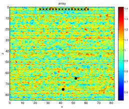
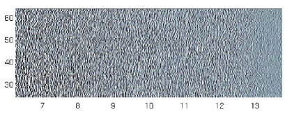
To illustrate how clutter impedes imaging, we present here the results of a numerical simulation in two dimensions, in the setup depicted on the left in Figure 1. There are two small reflectors to image, shown with the black dots. They are modeled as sound soft disks of radius $\lambda_{o}/4$, centered at $\vec{\mathbf{y}}_{1}=(42\lambda_{o},75\lambda_{o})$ and $\vec{\mathbf{y}}_{2}=(52\lambda_{o},65\lambda_{o})$. The array is linear, and consists of $N=80$ transducers. The range axis is orthogonal to it, and points downward in the figure. The transducer locations are

$$\vec{\mathbf{x}}_{r}=\left(x_{r},2\lambda_{o}\right),\quad x_{r}=24\lambda_{o}+(r-1)\frac{\lambda_{o}}{2},\quad r=1,\ldots,80,$$

so the array has aperture $a\approx 40\lambda_{o}$, which is about half the range of the reflectors.

The clutter is a realization of

$$\mu(\vec{\mathbf{x}})=\frac{1}{\sqrt{2}}\left[\mu_{i}(\vec{\mathbf{x}})+\mu_{l}\Big{(}z\Big{)}\right],$$ (3.1)

where $\mu_{i}$ and $\mu_{l}$ are mean zero, statistically homogeneous random processes. The first models an isotropic random medium with autocorrelation

$$\mathbb{E}[\mu_{i}(\vec{\mathbf{x}})\mu_{i}(\vec{\mathbf{x}}^{\prime})]=\left(1+\frac{|\vec{\mathbf{x}}-\vec{\mathbf{x}}^{\prime}|}{\ell}\right)e^{-\frac{|\vec{\mathbf{x}}-\vec{\mathbf{x}}^{\prime}|}{\ell}},$$ (3.2)

and correlation length $\ell=\lambda_{o}/4$. The second models a randomly layered medium with autocorrelation

$$\mathbb{E}[\mu_{l}(z)\mu_{l}(z^{\prime})]=\left(1+\frac{|z-z^{\prime}|}{\ell_{z}}\right)e^{-\frac{|z-z^{\prime}|}{\ell_{z}}},$$ (3.3)

and correlation length $\ell_{z}=\lambda_{o}/50$. The amplitude scale of the fluctuations $\mu(\vec{\mathbf{x}})$ is $\varepsilon=0.1$, and the actual wave speed $v(\vec{\mathbf{x}})$ used in the simulation is shown with colors in Figure 1.

The simulation parameters are typical for an ultrasonic non-destructive testing experiment [3]. The array probes the medium with Ricker pulses, which are second derivatives of a Gaussian, with central frequency $\omega_{o}/(2\pi)=10$MHz and standard deviation $10$MHz. The reference velocity is $c=1$Km/s, so $\lambda_{o}=0.1$mm. All the lengths in Figure 1 are scaled by $\lambda_{o}$.

The array response matrix ${\itbf{P}}(t)$ is obtained by solving numerically the wave equation (2.1) in $\mathbb{R}^{2}$, using the perfectly matched absorbing layer technique [8]. The numerical method uses a finite element discretization in space of (2.1), written as a first order hyperbolic system [6, 7]. The discretization in time is with standard finite differences.

We display on the right in Figure 1 the recordings $P(t,\vec{\mathbf{x}}_{r},\vec{\mathbf{x}}_{s})$ for $r=1,\ldots,80$ and $s=41$. Borrowing terminology from the seismic literature, we call the recordings time traces. The direct arrivals from the two sound soft disks are weak and cannot be seen because they are dominated by the clutter backscattered waves, which arrive before and after them.

(a) KM

(b) CINT

Fig. 2: Kirchhoff migration (a) and CINT (b) images obtained for the data shown on Figure 1(b). The full array response matrix is used to obtain these images and not just the central illumination data. The true location of the scatterers is shown with black circles.

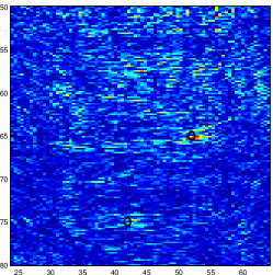
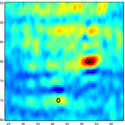
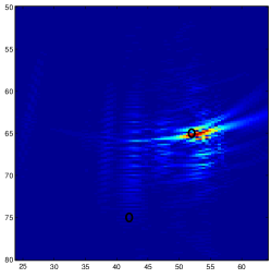
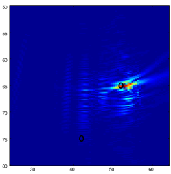
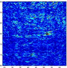
The KM and CINT images are shown in Figure 2, where the two sound soft reflectors are indicated with black circles. We note that both images have peaks near the locations of the reflectors. In particular, CINT produces a strong peak at the reflector that is closer to the array. However, there are many other peaks, which are stronger than the peak at the second reflector. The algorithm described in the next section is designed to mitigate the clutter backscatter, and therefore improve the quality of the images.

4 Detection and filtering of clutter backscatter

Our method of detection of the arrival of the weak echoes from the small reflectors, and of filtering the unwanted clutter backscatter, consists of two main parts, outlined here.

The first part is as in [15], and we review it in section 4.1. It analyzes the response matrix ${\itbf{P}}(t)$ in sequentially refined time windows using the discrete local cosine transform (LCT). Time windowing is useful because over the entire duration of the recordings the energy carried by the clutter backscatter (the ”noise”) overwhelms that of the useful echoes (the ”signal”). As the time windows containing these echoes become smaller and smaller, the signal to noise ratio (SNR) improves. The LCT allows a systematic window refinement and search, using a tree structure. It decomposes the entries of ${\itbf{P}}(t)$ over frequencies, locally in each window, and the detection is done by tracking the behavior of the leading singular values of the transformed matrix. Data filtering consists of zeroing the LCT coefficients in the windows where no signal is detected, projecting on the subspace spanned by the singular vectors of the distinguished singular values, and then inverting the LCT transform. We call the filtered response matrix ${\itbf{P}}^{{}^{TF}}(t)$, where the index TF stands for time filtering.

The second part of the method is the main contribution of this paper, and is described in section 4.2. It seeks to detect the direction of arrival of the desired echoes from the small reflectors, in addition to the arrival time, and to improve the data filter for better resolution of the images. To do so, we begin with the backpropagation of ${\itbf{P}}^{{}^{TF}}(t)$ using travel time delays from the array transducers to a reference point in the imaging region. This reference point is at range equal to half the center time of the selected time window, multiplied by the wave speed $c$. If more time windows are selected, than the backpropagation is done for each of them. The purpose of the backpropagation is to remove the large phase of the entries of ${\itbf{P}}^{{}^{TF}}(t)$, so that we can better analyze the data around the detected arrival time.

We call the backpropagated matrix ${\itbf{P}}^{{}^{BP}}(t)$ and its Fourier transform $\widehat{{\itbf{P}}}^{{}^{BP}}(\omega)$. Its entries are indexed by the receivers located at $\vec{\mathbf{x}}_{r}$ and sources at $\vec{\mathbf{x}}_{s}$, and we rotate it next by representing it in the center and difference coordinates $(\vec{\mathbf{x}}_{s}+\vec{\mathbf{x}}_{r})/2$ and $\vec{\mathbf{x}}_{r}-\vec{\mathbf{x}}_{s}$. The motivation for the rotation is similar to that in [3, 4, 2]. Assuming that the array aperture is small with respect to the range of the reflectors, we may use the paraxial approximation to model the direct arrivals from the small reflectors, the useful (coherent) part of the data. After the backpropagation, this part is approximately independent of the difference $\vec{\mathbf{x}}_{r}-\vec{\mathbf{x}}_{s}$, which is why it is advantageous to rotate $\widehat{{\itbf{P}}}^{{}^{BP}}(\omega)$.

We denote the rotation by $\mathcal{R}$, and to suppress the remaining clutter backscatter, we calculate the best approximation of $\mathcal{R}\widehat{{\itbf{P}}}^{{}^{BP}}(\omega)$ by a rank one matrix which is independent of $\vec{\mathbf{x}}_{r}-\vec{\mathbf{x}}_{s}$. The approximation is with respect to the Frobenius norm, and the result is denoted by $\mathcal{R}\widehat{{\itbf{P}}}^{{}^{AF}}(\omega)$.

To determine the direction of arrival of the coherent echoes i.e., the wave vectors associated with the single scattered waves, we decompose $\mathcal{R}\widehat{{\itbf{P}}}^{{}^{AF}}(\omega)$ in plane waves using Fourier transforms. The detection amounts to seeking maxima of the Fourier coefficients (the plane wave amplitudes), and the filtering is done by careful tapering over the other directions. The output of the algorithm is the inverse Fourier transform of the result, rotated back to the coordinates $\vec{\mathbf{x}}_{r}$ and $\vec{\mathbf{x}}_{s}$. This is the filtered data to be used in the image formation.

4.1 Adaptive time-frequency detection and filtering

We review here the steps of the algorithm introduced in [15]. The input is the array response matrix ${\itbf{P}}(t)$, for time $t\in[0,T]$ sampled in uniform $N_{T}$ time steps, where $N_{T}$ equals an integer power of $2$. The LCT decomposition [19] is done in time windows arranged in a binary tree structure. At each level $l=0,\ldots,N_{l}$, the recording window $[T_{o},T]$ is divided in $2^{l}$ windows, of size $\Delta_{l}=(T-T_{o})/2^{l}$. The minimum size of the time windows is determined by the user defined maximum tree level $N_{l}$.

Let us index the nodes of the tree by $(j,l)$, with $j=0,\ldots,2^{l}-1$ and $l=0,\ldots,N_{l}$. Each node is associated with the subspace spanned by the orthonormal bases

$$\mathscr{B}_{j}^{l}=\left\{\sqrt{\frac{2}{\Delta_{l}}}\chi\Big{(}\frac{t-t_{j}^{l}}{\Delta_{l}}\Big{)}\cos[\omega_{n}^{l}(t-t_{j}^{l})],~{}~{}n\in\mathbb{Z}^{+}\right\},$$ (4.1)

with discrete times $t_{j}^{l}=T_{o}+j\Delta_{l}$ and frequencies $\omega_{n}^{l}={\pi\left(n+1/2\right)}/{\Delta_{l}}$ of the decomposition in the smooth windows $\chi$. For any $l$, the union over $j$ of the bases $\mathscr{B}_{j}^{l}$ forms an orthonormal basis of $L^{2}[T_{o},T]$, and at the next tree level the span of $\mathscr{B}_{j}^{l}$ is split in two orthogonal subspaces, with bases $\mathscr{B}_{2j}^{l+1}$ and $\mathscr{B}_{2j+1}^{l+1}$. We refer to [19] for details.

The steps of the time-frequency detection and fitering algorithm are:

1. Computation of the discrete LCT transform of the array response matrix on a binary tree with maximum level $N_{l}$. This gives the $N\times N$ matrices

   $$\widehat{\itbf{P}}^{l}{(t_{j}^{l},\omega_{n}^{l})}=\left\{\widehat{P}^{l}(t_{j}^{l},\omega_{n}^{l},\vec{\mathbf{x}}_{r},\vec{\mathbf{x}}_{s})\right\}_{r,s=1,\ldots,N},$$ (4.2)

   for $j=0,1,\ldots,2^{l}-1$ and $l=0,\ldots,N_{l}$, with entries

   $$\widehat{P}^{l}(t_{j}^{l},\omega_{n}^{l},\vec{\mathbf{x}}_{r},\vec{\mathbf{x}}_{s})=\int dt\,P(t,\vec{\mathbf{x}}_{r},\vec{\mathbf{x}}_{s})\sqrt{\frac{2}{\Delta_{l}}}\chi\Big{(}\frac{t-t_{j}^{l}}{\Delta_{l}}\Big{)}\cos[\omega_{n}^{l}(t-t_{j}^{l})].$$ (4.3)

2. Calculate the singular value decomposition of $\widehat{\itbf{P}}^{l}{(t_{j}^{l},\omega_{n}^{l})}$. Let $\sigma^{l,j}_{q}(\omega_{n}^{l})$ be the singular values, for $q=1,\ldots N$.

3. Choose the frequency band $\mathcal{B}\in(0,\pi N_{T}/T)$ and the number $\bar{q}$ of largest singular values to be used in the detection.

4. Detect the time window of interest as follows:
   For $l=0:N_{l}$

   1. Decide if there is at least one window indexed by $(j,l)$, where the largest singular values are distinguished from the others across the frequencies in $\mathcal{B}$. If yes, let $l_{o}=l$ and $j_{\star}^{l_{o}}=j$ and stop.
      

   For $l=l_{0}+1:N_{l}$

   1. Let $j\in\{2j_{\star}^{l-1},2j_{\star}^{l-1}+1\}$ and decide in which of the two windows the largest singular values are better separated from the rest. Call the decision $j_{\star}^{l}=j$. If the selection is ambiguous, set $l=l-1$ and stop.

5. Let the chosen time window be indexed by $(j_{\star}^{l},l)$. Set to zero the LCT coefficients in all other windows at level $l$. This is equivalent to multiplying (4.3) with the Kronecker $\delta_{j,j_{\star}^{l}}$.

6. Project $\delta_{j,j_{\star}^{l}}\widehat{\itbf{P}}^{l}(t_{j}^{l},\omega_{n}^{l})$ on the subspace of low rank matrices with singular vectors corresponding to the distinguished top singular values. The projection is done for frequencies $\omega_{n}\in\mathcal{B}$. All other coefficients are set to zero.

7. The output of the algorithm is the filtered response matrix ${\itbf{P}}^{{}^{TF}}(t)$ obtained with the inverse LCT of the entries of the matrix obtained at step (6).

Remarks

The number $\bar{q}$ of singular values at step (3) should be larger than the number $M$ of reflectors that we wish to image. We also should have enough measurements, meaning that $N\gg\bar{q}>M$. The bandwidth ${\mathcal{B}}$ is the part of the frequency support of the probing pulse over which the reflectors are detectable. This ${\mathcal{B}}$ depends on the clutter, but in general it is at the lower frequencies that the detection is easier.

The details on how the algorithm searches for the distinguishable, leading singular values are given in [15]. Note that at step (4) we search first from the bottom to the top of the tree. At the root level $l=0$, the data is expected to be dominated by the clutter backscatter, so $\widehat{\itbf{P}}^{0}(T_{o},\omega_{n}^{0})$ are like noise matrices. This is illustrated in Figure 12 and the numerical simulations in [15] by the fact that all singular values $\sigma_{q}^{0,0}(\omega_{n}^{0})$ are clustered together across the frequencies. There is no distinguished or significant singular value. When the window sizes become small enough, the SNR in the windows that contain the useful echoes from the reflectors (the signal) improves, and the largest singular values become well separated from the others. This is the level $l_{o}$ at step (4). The second part of the search at step (4) refines sequentially the windows of interest until the selection becomes ambiguous.

The filters at steps (5) and (6) are for suppressing the clutter backscatter. First, they remove all the arrivals outside the selected time window and then, they project the result on the subspace spanned by the singular vectors corresponding to the distinguishable singular values.

4.2 Direction of arrival detection and filtering

The filtered array response matrix ${\itbf{P}}^{{}^{TF}}(t)$ given by the first part of the algorithm is localized in a small time window which contains the echoes from the reflectors that we wish to image. Here we explain how we can detect the direction of arrival of these echoes and how we can improve the data filtering.

Fig. 3: Illustration of an imaging setup with array aperture $a$ that is small compared to the range $L$. The reference point $\vec{\mathbf{y}}_{o}$ is determined from the center time of a selected window and is along the range axis originating at the center of the array.

Suppose that a small reflector at $\vec{\mathbf{y}}$ is detected in the selected time window centered at $t_{o}$. Its distance to the center of the array, the origin of coordinates, is approximately $L=c/(2t_{o})$, and we define the reference point $\vec{\mathbf{y}}_{o}=({\bf 0},L)$. As illustrated in Figure 3, $\vec{\mathbf{y}}_{o}$ is offset from $\vec{\mathbf{y}}$ by $\mathbf{y}$ in the cross-range plane and $\eta$ in range, meaning that $\vec{\mathbf{y}}=(\mathbf{y},L+\eta)$.

The useful echoes for imaging, which are single scattered at $\vec{\mathbf{y}}$, have the deterministic phase $k(|\vec{\mathbf{y}}-\vec{\mathbf{x}}_{s}|+|\vec{\mathbf{y}}-\vec{\mathbf{x}}_{r}|)$ for the source receiver pair $(s,r)$, where $k=\omega/c$ is the wavenumber. Assuming that the array is planar, with small aperture with respect to the range $L$, we let $\vec{\mathbf{x}}_{r}=(\mathbf{x}_{r},0)$ and obtain with the paraxial approximation that

$$|\vec{\mathbf{y}}-\vec{\mathbf{x}}_{s}|+|\vec{\mathbf{y}}-\vec{\mathbf{x}}_{r}| =\sqrt{(L+\eta)^{2}+|\mathbf{x}_{r}-\mathbf{y}|^{2}}+\sqrt{(L+\eta)^{2}+|\mathbf{x}_{s}-\mathbf{y}|^{2}}$$

$$\approx 2(L+\eta)+\frac{|\mathbf{x}_{r}-\mathbf{y}|^{2}+|\mathbf{x}_{s}-\mathbf{y}|^{2}}{2L}$$

$$=2(L+\eta)+\frac{|\bar{\mathbf{x}}_{rs}|^{2}}{L}+\frac{|\widetilde{\mathbf{x}}_{rs}|^{2}}{4L}+\frac{|\mathbf{y}^{2}|}{L}-\frac{2\bar{\mathbf{x}}_{rs}\cdot\mathbf{y}}{L},$$ (4.4)

where $\bar{\mathbf{x}}_{rs}=(\mathbf{x}_{r}+\mathbf{x}_{s})$ and $\widetilde{\mathbf{x}}_{rs}=\mathbf{x}_{r}-\mathbf{x}_{s}.$ For the reference point $\vec{\mathbf{y}}_{o}$ we have similarly

$$|\vec{\mathbf{y}}_{o}-\vec{\mathbf{x}}_{s}|+|\vec{\mathbf{y}}_{o}-\vec{\mathbf{x}}_{r}| =\sqrt{L^{2}+|\mathbf{x}_{r}|^{2}}+\sqrt{L^{2}+|\mathbf{x}_{s}|^{2}}$$

$$\approx 2L+\frac{|\bar{\mathbf{x}}_{rs}|^{2}}{L}+\frac{|\widetilde{\mathbf{x}}_{rs}|^{2}}{4L},$$ (4.5)

so when backpropagating the filtered data ${\itbf{P}}^{{}^{TF}}(t)$ to $\vec{\mathbf{y}}_{o}$ we achieve the following phase reduction of the direct arrivals in the selected time window

$$k(|\vec{\mathbf{y}}-\vec{\mathbf{x}}_{s}|+|\vec{\mathbf{y}}-\vec{\mathbf{x}}_{r}|-|\vec{\mathbf{y}}_{o}-\vec{\mathbf{x}}_{s}|+|\vec{\mathbf{y}}_{o}-\vec{\mathbf{x}}_{r}|)\approx k\left(2\eta+\frac{|\mathbf{y}^{2}|}{L}-\frac{2\bar{\mathbf{x}}_{rs}\cdot\mathbf{y}}{L}\right).$$ (4.6)

The observation that these reduced phases are independent of the difference coordinates $\widetilde{\mathbf{x}}_{rs}$ leads to the detection and filtering algorithm described below.

The algorithm can be used for three dimensional problems, but to avoid cumbersome index notation we present it here in two dimensions, for a linear array. The extension to three dimensions requires a modification of the indexing in the rotation operation at step (2) below. The steps of the algorithm are:

1. For the selected time window, centered at $t_{o}$, define the $N\times N$ input matrix

   $$\itbf{P}^{{}^{IN}}(t)=\itbf{P}^{{}^{TF}}(t-t_{o}),$$ (4.7)

   and Fourier transform it with respect to time $t$,

   $$\widehat{{\itbf{P}}}^{{}^{IN}}(\omega)=\int_{-\infty}^{\infty}e^{i\omega t}{\itbf{P}}^{{}^{IN}}(t)dt=e^{i\omega t_{o}}\int_{-\infty}^{\infty}e^{i\omega(t-t_{o})}\itbf{P}^{{}^{TF}}(t-t_{o})dt.$$ (4.8)

   Denote the entries of this matrix by $\widehat{P}^{{}^{IN}}(\omega,x_{r},x_{s})$, since for the linear array $\vec{\mathbf{x}}_{r}=(x_{r},0)$, with $r=1,\ldots,N$.

   Backpropagate $\widehat{{\itbf{P}}}^{{}^{IN}}(\omega)$ to the test point $\vec{\mathbf{y}}_{o}$, and denote the resulting matrix by $\widehat{{\itbf{P}}}^{{}^{BP}}(\omega)$, with entries defined by

   $$\widehat{P}^{{}^{BP}}(\omega,x_{r},x_{s})=\widehat{P}_{o}(\omega,x_{r},x_{s})e^{-i\omega t_{o}-ik(|\vec{\mathbf{y}}_{o}-\vec{\mathbf{x}}_{s}|+|\vec{\mathbf{y}}_{o}-\vec{\mathbf{x}}_{r}|)},\quad r,s=1,\ldots,N.$$ (4.9)

2. Rotate $\widehat{{\itbf{P}}}^{{}^{BP}}(\omega)$ by ninety degrees, to form a larger $(2N-1)\times(2N-1)$ matrix, with entries indexed by the center and difference coordinates

   $$\bar{x}_{rs}=\frac{x_{r}+x_{s}}{2},\quad\widetilde{x}_{rs}=x_{r}-x_{s}.$$

   The rotation is done with the following commands:

   ⬇

   $\itbf{H}=\widehat{{\itbf{P}}}^{{}^{BP}}(\omega)$

   ${\mathcal{R}}\itbf{H}=zeros(2N-1,2N-1)$

   For i=1:N

   For j=1: N

   i1=i+j-1

   i2=i-j-(1-N)+1

   $\mathcal{R}$H(i1,i2)= H(j,i)

   end

   end

   The rotated matrix has a rhombus structure as illustrated in Figure 4. The diagonals in $\itbf{H}$, which correspond to constant source receiver offsets $\widetilde{x}_{rs}$, form the columns of $\mathcal{R}\itbf{H}$. The anti-diagonals of $\itbf{H}$, which correspond to common midpoints $\bar{x}_{rs}$, form the rows of $\mathcal{R}\itbf{H}$. The resulting matrix is $\mathcal{R}\widehat{{\itbf{P}}}^{{}^{BP}}(\omega)$.

   

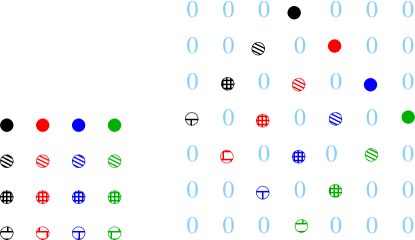
   Fig. 4: Illustration of a square $4\times 4$ matrix $\itbf{H}$ on the left and its rotation ${\mathcal{R}}\itbf{H}$ on the right.

3. We know from equation (4.6) that the desired, coherent part of the matrix calculated at step (2) should be independent of the source receiver offsets $\widetilde{x}_{rs}$. Therefore, we calculate the best approximation of ${\mathcal{R}}\widehat{{\itbf{P}}}^{{}^{BP}}(\omega)$ by a matrix $\mathcal{R}\widehat{{\itbf{P}}}^{{}^{AF}}(\omega)$ with identical columns $\widehat{\itbf{p}}(\omega)$, restricted to the support of ${\mathcal{R}}\widehat{{\itbf{P}}}^{{}^{BP}}(\omega)$, i.e., the non-zero elements of the rhombus. Let $\mathscr{S}$ be the set of indexes $(i,j)$ in this support, for $i,j=1,\ldots,2N-1$ enumerating the center and difference locations, renamed henceforth $\bar{x}_{i}$ and $\widetilde{x}_{j}$, and define the indicator function

   $$1_{{}_{\mathscr{S}}}(i,j)=\left\{\begin{array}[]{ll}1,&(i,j)\in\mathscr{S}\\ 0,&\mbox{otherwise}\end{array}\right..$$

   Then, $\widehat{\itbf{p}}(\omega)$ is the $2N-1$ column vector with entries $p(\omega,\bar{x}_{i})$ that minimize

   $$\sum_{i,j=1}^{2N-1}1_{{}_{\mathscr{S}}}(i,j)\left|{\mathcal{R}}\widehat{P}^{{}^{BP}}(\omega,\bar{x}_{i},\widetilde{x}_{j})-\widehat{p}(\omega,\bar{x}_{i})\right|^{2}.$$

   We obtain that

   $$\widehat{p}(\omega,\bar{x}_{i})=\frac{1}{n_{i}}\sum_{j=1}^{2N-1}{\mathcal{R}}\widehat{P}^{{}^{BP}}(\omega,\bar{x}_{i},\widetilde{x}_{j}),\quad n_{i}=\sum_{j=1}^{2N-1}1_{{}_{\mathscr{S}}}(i,j),$$ (4.10)

   where $n_{i}$ is is the number of non zero entries of the $i-$th row in the set $\mathscr{S}$. Here we used that $\mathcal{R}\widehat{{\itbf{P}}}^{{}^{BP}}(\omega)$ is supported in $\mathscr{S}$.

   The approximation $\mathcal{R}\widehat{{\itbf{P}}}^{{}^{AF}}(\omega)$ is the matrix with entries

   $$\mathcal{R}\widehat{P}^{{}^{AF}}(\omega,\bar{x}_{i},\widetilde{x}_{j})=1_{{}_{\mathscr{S}}}(i,j)\widehat{p}(\omega,\bar{x}_{i}),\quad i,j=1,\ldots,2N-1.$$ (4.11)

4. Take the Fourier transform of (4.10) with respect to $\bar{x}$. This is a plane wave decomposition, with wave vector samples $\kappa_{i}$, the dual variable to $\bar{x}_{i}$. The transformed vector is

   $$\breve{\itbf{p}}(\omega)=\left(\breve{p}(\omega,\kappa_{i})\right)_{i=1,\ldots,2N-1}.$$ (4.12)

5. The detection of the direction of arrival of the direct echoes from the reflectors amounts to seeking maxima of (4.12) that are above a user defined tolerance. If there is one dominant reflector for the selected time window, we expect a single maximum, denoted by $\kappa^{\star}(\omega)$. For multiple reflectors we may have multiple maxima. If they are well separated, we use them one at a time.

6. To filter the residual unwanted clutter backscatter, we taper off the arrivals from the directions that are different than the selected $\kappa^{\star}(\omega)$ at step (5). The taper function is determined by the aperture $a$ of the array, which defines the resolution of order $a/L$ in the plane wave decomposition.

   In theory, the taper should be a sinc function, due to the support of the entries of $\widehat{\itbf{p}}(\omega)$ in the interval $[-a/2,a/2]$. Since we are interested only in the vicinity of the peak wave vector, we taper using a Gaussian centered at $\kappa^{\star}(\omega)$, with standard deviation $\beta$ determined by minimizing the least squares error between $\breve{p}(\omega,\kappa_{i})$ and $\breve{p}(\omega,\kappa_{i})\exp[-(\kappa_{i}-\kappa_{i}^{\star})^{2}/(2\beta^{2})]$ in the vicinity of $\kappa^{\star}$, where $\breve{p}(\omega,\kappa_{i})$ drops up to half of its peak value.

   We denote the tapered vector by $\breve{\itbf{p}}^{{}^{DoA}}(\omega)$, with index DoA standing for direction of arrival. Its entries are defined by

   $$\breve{{p}}^{{}^{DoA}}(\omega,\kappa_{i})=\breve{p}(\omega,\kappa_{i})e^{-\frac{[\kappa_{i}-\kappa^{\star}(\omega)]^{2}}{2\beta^{2}}},\quad i=1,\ldots,2N-1.$$ (4.13)

7. Compute the inverse Fourier transform (with respect to $\kappa$) of the tapered vector (4.13). Its entries are

   $$\widehat{{p}}^{{}^{\,DoA}}(\omega,\bar{x}_{i})\sim\widehat{p}(\omega,\bar{x}_{i})\star_{\bar{x}}e^{i\kappa^{\star}(\omega)\bar{x}_{i}-\frac{\beta^{2}\bar{x}_{i}^{2}}{2}},$$

   where $\star_{\bar{x}}$ denotes convolution and $\sim$ denotes equal, up to a multiplicative constant. The phase in the right hand side of this equation carries the direction of arrival selected at step (6).

8. Define the filtered, rotated matrix $\mathcal{R}\widehat{\itbf{P}}^{{}^{DoA}}(\omega)$, with entries

   $$\mathcal{R}\widehat{P}^{{}^{DoA}}(\omega,\bar{x}_{i},\widetilde{x}_{j})=1_{{}_{\mathscr{S}}}(i,j)\widehat{p}^{{}^{\,DoA}}(\omega,\bar{x}_{i}),\quad i,j=1,\ldots,2N-1.$$ (4.14)

   Rotate it back to obtain the $N\times N$ matrix $\widehat{\itbf{P}}^{{}^{DoA}}(\omega)$ with entries $\widehat{P}^{{}^{DoA}}(\omega,x_{r},x_{s})$, for $r,s=1,\ldots,N$.

9. Undo the back propagation at step (1), equation (4.9), by multiplying  
   $\widehat{P}^{{}^{DoA}}(\omega,x_{r},x_{s})$ with $\exp\left[i\omega t_{o}+ik(|\vec{\mathbf{y}}_{o}-\vec{\mathbf{x}}_{s}|+|\vec{\mathbf{y}}_{o}-\vec{\mathbf{x}}_{r}|)\right]$, for $r,s=1,\ldots,N$.

10. The output of the algorithm is the inverse Fourier transform in time of the matrix calculated at step (9). We call it ${\itbf{P}}^{{}^{OUT}}(t)$.

Remarks

Equation (4.6), which states that after the backpropagation the direct echoes from the sought-after reflectors carry phases that are independent of the source-receiver offset location, is used by the algorithm in two ways: First, it rotates at step (2) the backpropagated data matrix to the center and difference system of coordinates $\bar{x}_{i}$, and $\widetilde{x}_{j}$, and then approximates at step (3) the result by the closest matrix with identical columns, independent of the offset coordinates $\widetilde{x}_{j}$. Second, it Fourier transforms the result with respect to the center coordinates $\bar{x}_{i}$, to determine at steps (4) and (5) the wave vector $\kappa^{\star}(\omega)$ corresponding to the desired direct echoes. Equation (4.6) says that this should be approximately $\kappa^{\star}(\omega)\approx 2ky/L.$ The algorithm then suppresses the returns with wave vectors away from $\kappa^{\star}(\omega)$ at step (6). The remaining steps (7)-(9) undo the rotation and the Fourier transform to return to the source-receiver coordinates and the time domain in which the array response matrix is represented.

As stated before, the algorithm applies to three dimensions, with the only difference being in the indexing in the rotation operation at step (2), and the search for the direction of arrival at step (5) in two dimensions instead of one.

5 Numerical simulations

We begin in section 5.1 with the illustration of the direction of arrival detection and filtering algorithm, for the setup considered in section 3. Then we present in section 5.2 imaging results for two nearby reflectors in three location arrangements and three different types of clutter.

Fig. 5: From left to right: the real part of $\widehat{{\itbf{P}}}^{{}^{BP}}(\omega)$, its approximation by the Hankel matrix $\widehat{{\itbf{P}}}^{{}^{AF}}(\omega)$ and the filtered matrix $\widehat{{\itbf{P}}}^{{}^{OUT}}(\omega)$. The axes are the indexes of the transducers and $\omega/(2\pi)=5$MHz.

5.1 Illustration of direction of arrival detection and filtering

The numerical simulations in this section are for the setup illustrated in Figure 1 and described in detail in section 3. We focus attention on the reflector that is closer to the array, and illustrate how the algorithm introduced in section 4.2 detects the arrival of the direct echoes from it and removes the clutter backscatter.

Since there are $N=80$ transducers in the simulation, the array response matrix ${\itbf{P}}(t)$ is of size $80\times 80$, and the time recordings are $N_{T}=2^{13}$ for the duration $T-T_{o}=13.7748$$\mu$s. We start the recordings at time $T_{o}=6.2252$$\mu$s and end them at time $T=20$$\mu$s. The selection of the time window containing the arrival of the direct echoes is done as explained in section 4.1 and described in detail in [15]. It identifies the window at the level $l=4$ of the LCT tree, indexed by $j_{\star}^{4}=7,$ and centered at time

$$t_{o}=T_{o}+(j_{\star}^{4}+1/2)\Delta_{4},\quad\Delta_{4}=(T-T_{o})/2^{4}.$$

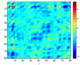
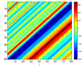
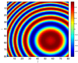
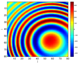
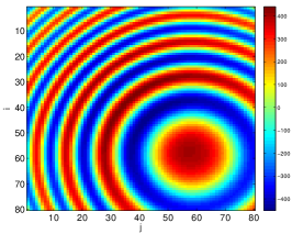
The direction of arrival detection and filtering begins with the matrix ${\itbf{P}}^{{}^{IN}}(t)$ defined in equation (4.8). We Fourier transform it and backpropagate it to the reference point $\vec{\mathbf{y}}_{o}=(0,c/(2t_{o}))$ using equation (4.9), and display in the left plot of Figure 5 the real part of the resulting matrix $\widehat{{\itbf{P}}}^{{}^{BP}}(\omega)$, at frequency $\omega/(2\pi)=5$MHz. In the middle plot we display its approximation $\widehat{{\itbf{P}}}^{{}^{AF}}(\omega)$ obtained by rotating the matrix defined in equation (4.11) to the system of coordinates corresponding to the source and receiver locations. This is a Hankel matrix by construction. In the right plot we display the filtered matrix $\widehat{{\itbf{P}}}^{{}^{OUT}}(\omega)$, the Fourier transform of the output matrix at step (9) of the algorithm. We compare it in Figure 6 with the ideal array response matrix in the homogeneous medium, which has rank one and entries

$$\widehat{P}^{{}^{HOM}}(\omega,\vec{\mathbf{x}}_{r},\vec{\mathbf{x}}_{s})=\frac{e^{ik\left(|\vec{\mathbf{x}}_{r}-\vec{\mathbf{y}})+|\vec{\mathbf{x}}_{s}-\vec{\mathbf{y}}|\right)}}{16\pi^{2}|\vec{\mathbf{x}}_{r}-\vec{\mathbf{y}}||\vec{\mathbf{x}}_{s}-\vec{\mathbf{y}}|}.$$

We note that the matrices are quite close, so the filtering algorithm works well. In the right plot of Figure 6 we display the rank one approximation of $\widehat{{\itbf{P}}}^{{}^{OUT}}(\omega)$, the matrix with the leading left and right singular vectors and singular value of $\widehat{{\itbf{P}}}^{{}^{OUT}}(\omega)$. The improvement is slight, and has little effect on the images displayed in Figure 7. Comparing these images with those in Figure 2 we note the dramatic improvement brought by the filtering algorithm.

Fig. 6: From left to right: the real part of the ideal response matrix $\widehat{{\itbf{P}}}^{{}^{HOM}}(\omega)$ in the homogeneous medium, the filtered matrix $\widehat{{\itbf{P}}}^{{}^{OUT}}(\omega)$, and its rank one approximation. The axes are the indexes of the transducers and $\omega/(2\pi)=5$MHz.

Fig. 7: Kirchhoff migration images formed with the filtered data matrix ${{\itbf{P}}}^{{}^{OUT}}(t)$ (left) and the inverse Fourier transform of its rank one approximation (right). They are almost the same. The abscissa is cross-range in units of $\lambda_{o}$ and the ordinate is range in units of $\lambda_{o}$.

Fig. 8: We display the absolute value of the entries of $\breve{\itbf{p}}(\omega)$ defined in equation (4.12) (blue line) and the Gaussian taper in green. The points used to determine the least squares fit by the Gaussian at step (6) are shown with green stars. The abscissa is scaled by the wavenumber $k$ so the peak corresponds to $2y/L$.

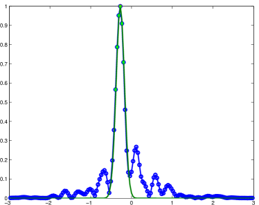
To illustrate the use of the rotation and approximation at step (3) of the algorithm, equation (4.10) in particular, we plot in Figure 8 the entries of the vector $\breve{\itbf{p}}(\omega)$ as a function of $\kappa$. We note that there is a clear peak, corresponding to the arrival of the coherent echoes from the reflector at $\vec{\mathbf{y}}$, that is fitted with the Gaussian taper shown in green.

5.2 Imaging two reflectors in different geometrical configurations and types of clutter

We assess in this section the performance of the direction of arrival filtering algorithm for different geometric configurations of two reflectors and different cluttered media, as illustrated in Figures 9 and 10. We begin with the numerical setup in section 5.2 and then we show the results in the following sections.

5.2.1 Description of the numerical setup

Fig. 9: Combined cluttered medium modeled by the process $\mu$ in equation (3.1). Three configurations of two reflectors. We call them configurations 1, 2 and 3 from left to right.

Fig. 10: The third configuration of reflectors in three different cluttered media. Isotropic on the left, layered in the middle and combined on the right.

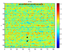
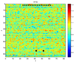
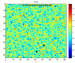
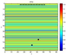
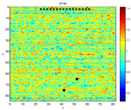
We consider three geometrical arrangements of two reflectors which are offset either in range, in cross-range or both directions, as illustrated in Figure 9. The reflectors are sound soft disks of radius $\lambda_{o}/4$, located at $\vec{\mathbf{y}}_{1}=(37\lambda_{o},65\lambda_{o})$, $\vec{\mathbf{y}}_{2}=(37\lambda_{o},72\lambda_{o})$ for configuration 1, at $\vec{\mathbf{y}}_{1}=(42\lambda_{o},75\lambda_{o})$, $\vec{\mathbf{y}}_{2}=(52\lambda_{o},75\lambda_{o})$ for configuration 2, and at $\vec{\mathbf{y}}_{1}=(42\lambda_{o},75\lambda_{o})$, $\vec{\mathbf{y}}_{2}=(52\lambda_{o},65\lambda_{o})$ for the third configuration.

We test the direction of arrival filtering algorithm in three different types of clutter modeled by the isotropic random process $\mu_{i}$ in equation (3.2), the layered one $\mu_{l}$ in equation (3.3), and the combined $\mu$ in equation (3.1). In all cases, the smooth part of the speed is constant $c=1$km/s, and the fluctuations are generated with random Fourier series. In the isotropic medium the standard deviation of the fluctuations is $\varepsilon=0.1$ and the correlation length is $\ell=\lambda_{o}/4$. For the layered medium $\varepsilon=0.17$ and $\ell=\lambda_{o}/50$. For the combined medium (3.1) the standard deviation is $\varepsilon=0.1$. We display in Figure 10 the realizations of the wave speed used in the simulations.

The array is linear, as described in section 3, and gathers the response matrix by probing the medium with one source at a time, emitting the same Ricker pulse. The receivers record the echoes in the time window $[T_{o},T]$ with $T_{o}=6.2252$$\mu$s and $T=20$$\mu$s. The time discretization is with $N_{T}=2^{13}$ steps.

5.2.2 Imaging results for the three reflector configurations

We present here imaging results in the clutter modeled by the process $\mu$ in equation (3.1), for the three geometric arrangements of the reflectors. We begin with Figure 11, where we display the KM images formed with the unfiltered response matrix ${\itbf{P}}(t)$. Due to the strong clutter, the images are noisy and difficult to interpret. Repeated simulations, in different realizations of $\mu$, also show that the images change dramatically, and unpredictably. We do not show the CINT images because they are also not useful in this strong clutter, as illustrated in Figure 2.

Fig. 11: KM images for the three configurations and clutter shown in Figure 9. The images are formed with the unfiltered response matrix ${\itbf{P}}(t)$. The abscissa is cross-range in units of $\lambda_{o}$ and the ordinate is range in units of $\lambda_{o}$. The reflectors are indicated with the black circles.

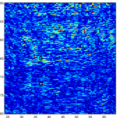
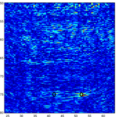
The first part of the filtering algorithm selects the time windows that contain the direct arrivals from the reflectors, at level $l=4$ in the LCT tree. They are indexed by $j_{\star}^{4}=7$ and $j_{\star}^{4}=9$ in configurations 1 and 3 and by $j_{\star}^{4}=9$ in configuration 2, where a single window is selected. This is because in the second configuration the reflectors are at the same range location.

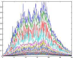
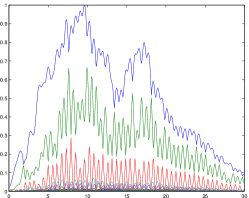
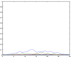
To illustrate the benefit of time windowing, we plot in Figure 12 the singular values of the array response matrix for the second configuration, at level 0 of the LCT tree, and then at level 4 for windows $j_{\star}^{4}=9$ and $j_{\star}^{4}=15$. The first window is selected by the algorithm as containing echoes from a reflector, and the second contains just clutter backscatter. We note that it is more difficult to distinguish the singular values at the root level, because they are clustered together. In the selected time window there is a clear separation of the larger singular values, signaling the arrival of the coherent echoes. In the last window, containing the clutter backscatter, the singular values are smaller and clustered together.

$j_{\star}^{0}=1$                            $j_{\star}^{4}=9$                            $j_{\star}^{4}=15$

Fig. 12: The singular values of the array response matrix as a function of frequency for configuration 2 in the combined medium. The left plot is at root level $l=0$ of the LCT tree i.e., for the entire duration of the recordings. The other plots are at the level $l=4$ of the tree, corresponding to $2^{4}$ time windows in the recording interval. The middle plot is for the selected window indexed by $j_{\star}^{4}=9$ which contains direct echoes from one of the reflectors. The right plot is for the unselected window indexed by $j_{\star}^{4}=15$ which contains only clutter backscatter. The plots are normalized by dividing the singular values at each tree level $l$ by the maximum one over all windows and frequencies at level $l$.

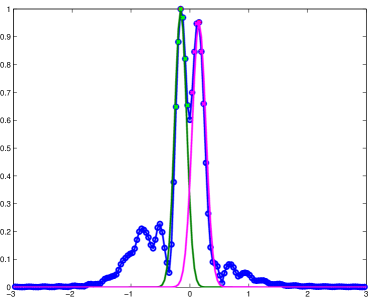
The input matrix ${\itbf{P}}^{{}^{IN}}(t)$ of the detection of the direction of arrival and filtering algorithm introduced in section 4.2 is calculated using equation (4.7), for each selected window centered at $t_{o}=T_{o}+(j_{\star}^{4}+1/2)\Delta_{4}$, with $\Delta_{4}=(T-T_{o})/2^{4}$. The images displayed below are formed with the filtered matrix ${\itbf{P}}^{{}^{OUT}}(t)$, the output of the algorithm. The direction of arrival selection at step (5) is as easy as in Figure 8 in configurations 1 and 3, because the selected time windows contain the direct echoes form a single reflector. In the second configuration the echoes from both reflectors arrive in the selected window, and the plot of the vector $\breve{\itbf{b}}(\omega)$ calculated at step (4) is shown in Figure 13. There are two peaks, corresponding to the direction of each reflector.

Fig. 13: Absolute value of the entries of $\breve{\itbf{p}}(\omega)$ defined in equation (4.12) (blue line) and the Gaussian tapers in green and pink. The points used to determine the least squares fit by the Gaussian at step (6) of the algorithm are shown with green and pink stars. The abscissa is scaled by the wavenumber $k$.

Fig. 14: Imaging results for configuration 1 and the clutter shown in Figure 9. Top row the images obtained with the data in the first selected time window and bottom row in the second selected time window. Left column: KM images formed with ${\itbf{P}}^{{}^{IN}}(t)$. Center column: KM images formed with ${\itbf{P}}^{{}^{OUT}}(t)$. Right column: CINT images formed with ${\itbf{P}}^{{}^{OUT}}(t)$. The abscissa is cross-range in units of $\lambda_{o}$ and the ordinate is range in units of $\lambda_{o}$.

Fig. 15: Imaging results for configuration 3 and the clutter shown in Figure 9. Top row the images obtained with the data in the first selected time window and bottom row in the second selected time window. Left column: KM images formed with ${\itbf{P}}^{{}^{IN}}(t)$. Center column: KM images formed with ${\itbf{P}}^{{}^{OUT}}(t)$. Right column: CINT images formed with ${\itbf{P}}^{{}^{OUT}}(t)$. The abscissa is cross-range in units of $\lambda_{o}$ and the ordinate is range in units of $\lambda_{o}$.

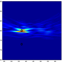
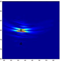
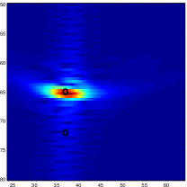
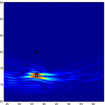
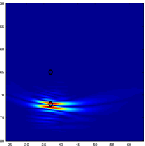
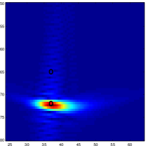
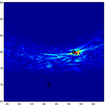
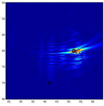
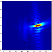
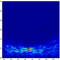
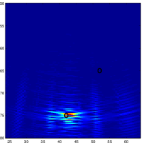
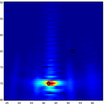
The imaging results for configurations 1 and 3 are shown in Figures 14 and 15, and are a significant improvement over those in Figure 11. Because the direct echoes from the reflectors are well separated in time and are captured in two different windows, we image one reflector at a time. The images are good even before the filtering over the direction of arrival, but this filtering sharpens the focusing of the images, specially in the third configuration.

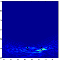
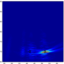
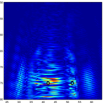
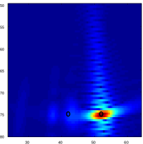
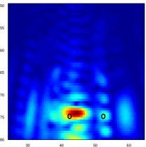
The direction of arrival filtering is important in the second configuration, where the echoes from both reflectors arrive in the same time window. Without it, only one reflector can be seen in the left image in Figure 16. The CINT method performs better than KM, as it mitigates the reverberations between the reflectors and the medium in their vicinity, as seen in the plots in the second row of the figure.

Fig. 16: Imaging results for configuration 2 and the clutter shown in Figure 9. There is a single selected time window containing the echoes from both reflectors. Left column: KM image formed with ${\itbf{P}}^{{}^{IN}}(t)$. Top row middle and right column: KM images formed with the filtered matrices ${\itbf{P}}^{{}^{OUT}}(t)$ for the two selected arrival directions in Figure 13. Bottom row: CINT images formed with ${\itbf{P}}^{{}^{OUT}}(t)$ for the two selected arrival directions. The abscissa is cross-range in units of $\lambda_{o}$ and the ordinate is range in units of $\lambda_{o}$.

5.2.3 Imaging results for different types of clutter

Fig. 17: Imaging results for configuration 2 in the layered clutter. Left column: KM image formed with ${\itbf{P}}^{{}^{IN}}(t)$. Top row middle and right column: KM images formed with the filtered matrices ${\itbf{P}}^{{}^{OUT}}(t)$ for the two selected arrival directions. Bottom row: CINT images formed with ${\itbf{P}}^{{}^{OUT}}(t)$ for the two selected arrival directions. The abscissa is cross-range in units of $\lambda_{o}$ and the ordinate is range in units of $\lambda_{o}$.

Fig. 18: Imaging results for configuration 2 in the isotropic clutter. Left column: KM image formed with ${\itbf{P}}^{{}^{IN}}(t)$. Top row middle and right column: KM images formed with the filtered matrices ${\itbf{P}}^{{}^{OUT}}(t)$ for the two selected arrival directions. Bottom row: CINT images formed with ${\itbf{P}}^{{}^{OUT}}(t)$ for the two selected arrival directions. The abscissa is cross-range in units of $\lambda_{o}$ and the ordinate is range in units of $\lambda_{o}$.

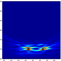
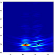
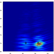
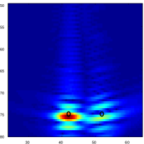
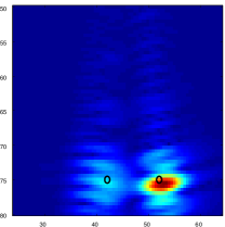
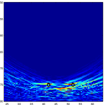
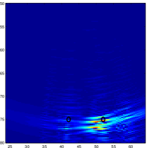
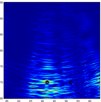
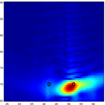
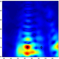
We display in Figures 17 and 18 the images of the two reflectors in the more difficult configuration 2, in layered and isotropic clutter, respectively. These complement the images in Figure 16. We note that the results are better in the layered case, as expected, because scattering in such clutter does not scramble the direction of the arrivals. This is why we can clearly see both reflectors in the KM image formed with the matrix ${\itbf{P}}^{{}^{IN}}(t)$. The direction of arrival filtering does not improve the focusing of the images, it just separates the two reflectors. In the isotropic clutter the imaging is more difficult, and the direction of arrival filtering is essential for focusing the images on the reflectors. As was the case in Figure 16, CINT gives slightly better images, because it mitigates the reverberations between the reflectors and the nearby clutter.

6 Summary

We introduced and tested with numerical simulations a novel detection and data filtering method for coherent array imaging of small reflectors in strongly scattering media, called heavy clutter. The array is a collection of $N$ transducers which play the double role of sources and receivers. It uses the sources to probe the medium with pulses and records the scattered waves. The data is organized in the $N\times N$ response matrix ${\itbf{P}}(t)$, which is a function of time. Because the medium reverberations (the clutter backscatter) dominate the recordings, it is difficult to distinguish the sought-after reflectors in the coherent images formed with ${\itbf{P}}(t)$. These are noisy and difficult to interpret because they change from one clutter to another.

The clutter is not known in imaging applications, which is why we model the uncertainty of the wave speed in the medium with a random process. A good imaging method must produce results that are insensitive to the realizations of the random wave speed i.e., be statistically stable. When the direct (coherent) arrivals of the waves scattered at the reflectors are strong enough with respect to the clutter backscatter, statistically stable imaging can be achieved with the coherent interferometric method (CINT) [14]. Here we consider much stronger clutter, that cannot be handled by CINT alone.

The detection and filtering method introduced in this paper is an improvement of that in [15]. It determines both the arrival time and direction of the weak coherent echoes, and suppresses all the other arrivals, which are clutter backscatter. The arrival time detection involves an adaptive time-frequency analysis of the response matrix in sequentially refined time windows, using the singular value decomposition (SVD) of the local cosine transform (LCT) of ${\itbf{P}}(t)$. The SVD of the Fourier transformed matrix $\widehat{{\itbf{P}}}(\omega)$ has been used to improve imaging in many works, see for example [20]. However, in our context it is not useful by itself, because the clutter backscatter carries most of the energy over the duration of the recordings. Therefore $\widehat{{\itbf{P}}}(\omega)$ is essentially a ”noise” matrix, with no distinguishable singular values. Our method uses the SVD in combination with the LCT analysis, to search systematically for the time windows in which the coherent echoes arrive. These echoes are distinguishable from the clutter backscatter with the SVD, when the time windows are small enough.

The detection of the direction of arrival of the coherent echoes is carried in the selected time windows, using their paraxial approximation. This approximation is justified for array apertures that are small with respect to the distance from the array to the reflectors, as is usually the case in practice. To use the paraxial approximation, we localize the data in time by backpropagating it to a reference point defined by the center time of the selected time windows, using travel time delays. This eliminates the large phase of the coherent echoes and more importantly, it removes their dependence on the source and receiver location offsets in the array. That is to say, it makes the coherent part of the backpropagated data a Hankel matrix. The method exploits this fact by seeking the best approximation of the backpropagated data matrix by a Hankel matrix, and then uses plane wave decompositions of the result to detect the direction of arrival of the desired coherent echoes. This leads to improved focusing of images, as shown with numerical simulations carried in a realistic setup motivated by the application of non-destructive testing.

References

- [1] R. Alonso, L. Borcea, G. Papanicolaou, and C. Tsogka. Detection and imaging in strongly backscattering randomly layered media. Inverse Problems, 27:025004, 2011.
- [2] A. Aubry and A. Derode. Detection and imaging in a random medium: A matrix method to overcome multiple scattering and aberration. J.APPL.PHYS., 106:044903, 2009.
- [3] A. Aubry and A. Derode. Random matrix theory applied to acoustic backscattering and imaging in complex media. Phys. Rev. Lett., 102(8):084301, Feb 2009.
- [4] A. Aubry and A. Derode. Singular value distribution of the propagation matrix in random scattering media. Waves in Random and Complex Media, 20:333–363, 2010.
- [5] A. Bakulin and R. Calvert. The virtual source method: Theory and case study. Geophysics, 71:SI139–SI150, 2006.
- [6] E. Bécache, P. Joly, and C. Tsogka. Etude d’un nouvel élément fini mixte permettant la condensation de masse. C. R. Acad. Sci. Paris Sér. I Math., 324:1281–1286, 1997.
- [7] E. Bécache, P. Joly, and C. Tsogka. An analysis of new mixed finite elements for the approximation of wave propagation problems. SIAM J. Numer. Anal., 37:1053–1084, 2000.
- [8] J. Bérenger. A perfectly matched layer for the absorption of electromagnetic waves. Journal of Comp. Physics, 114:185–200, 1994.
- [9] Biondo Biondi. 3D Seismic Imaging. Number 14 in Investigations in Geophysics. Society of Exploration Geophysicists, Tulsa, 2006.
- [10] N. Bleistein, J.K. Cohen, and J.W. Stockwell Jr. Mathematics of multidimensional seismic imaging, migration, and inversion. Springer, New York, 2001.
- [11] L. Borcea, F. González del Cueto, G. Papanicolaou, and C. Tsogka. Filtering random layering effects in imaging. SIAM Multiscal Modeling and Simulations, 8(3):751–781, 2010.
- [12] L. Borcea, J. Garnier, G. Papanicolaou, and C. Tsogka. Enhanced statistical stability in coherent interferometric imaging. Inverse Problems, 27:085004, 2011.
- [13] L. Borcea, G. Papanicolaou, and C. Tsogka. Interferometric array imaging in clutter. Inverse Problems, 21(4):1419–1460, 2005.
- [14] L. Borcea, G. Papanicolaou, and C. Tsogka. Adaptive interferometric imaging in clutter and optimal illumination. Inverse Problems, 22(4):1405–1436, 2006.
- [15] L. Borcea, G. Papanicolaou, and C. Tsogka. Adaptive time-frequency detection and filtering for imaging in heavy clutter. SIAM Imaging Science, 4(3):827–849, 2011.
- [16] Liliana Borcea, George Papanicolaou, and Chrysoula Tsogka. Asymptotics for the space-time Wigner transform with applications to imaging. Stochastic Differential Equations: Theory and Applications, Interdiscip. Math. Sci, 2:91–112, 2007.
- [17] D. Donoho, A. Maleki, and M. Shahram. Wavelab 850. http://www-stat.stanford.edu/~wavelab/, 2005.
- [18] J. Garnier, G. Papanicolaou, A. Semin, and C. Tsogka. Signal to Noise Ratio analysis in virtual source array imaging. SIAM Imaging Science, 8:248–279, 2015.
- [19] S. Mallat. A wavelet tour of signal processing. Academic Press, second edition, 1999.
- [20] C. Prada and M. Fink. Eigenmodes of the time reversal operator: A solution to selective focusing in multiple-target media. Wave Motion, 20:151–163, 1994.