Parabolic free boundary price formation models under market size fluctuations

Peter Markowich 4700 King Abdullah University of Science and Technology, Thuwal 23955-6900, Kingdom of Saudi Arabia Josef Teichmann Department of Mathematics, ETH Zürich, Rämistr. 101, 8092 Zürich, Switzerland  and  Marie-Therese Wolfram Mathematics Institute, University of Warwick, Coventry CV4 7TL, UK and Radon Institute for Computational and Applied Mathematics, Austrian Academy of Sciences, Altenbergerstr. 69, 4040 Linz, Austria. m.wolfram@warwick.ac.uk
Abstract.

In this paper we propose an extension of the Lasry-Lions price formation model which includes fluctuations of the numbers of buyers and vendors. We analyze the model in the case of deterministic and stochastic market size fluctuations and present results on the long time asymptotic behavior and numerical evidence and conjectures on periodic, almost periodic and stochastic fluctuations. The numerical simulations extend the theoretical statements and give further insights into price formation dynamics.

1. Introduction

This paper studies the impact of buyer and vendor number fluctuations on the price dynamics in an economic market in which a single good is traded. In general the formation of the price is a complex process, which results from the interplay of various additional factors such as trading behavior and rules, transaction costs, etc. Understanding these complicated interactions is a central research question in the field of market microstructure, which aims to explain “the process and outcome of exchanging assets under a specific set of rules” (see for example O’Hara [19]).
In 2007 Lasry and Lions introduced a minimalistic mean-field model (a one-dimensional parabolic free-boundary partial differential equation) to describe the price, which enters as the free boundary, of a single good traded between a large group of vendors and a large group of buyers.
Here we study a dynamic trading model, which is motivated by the price formation model proposed by Lasry and Lions. The original model considers a large group of buyers and vendors trading a single good. Each buyer or vendor acts continuously in time with his/her pre-trade price. If no trade takes place, the price diffuses instantaneously into its immediate neighborhood. When (through the diffusion around the pre-trade price) a buyer and vendor transact at this price, trading takes place. The buyer becomes a vendor, at a price which is the trading price plus the transaction cost, and the vendor becomes a buyer at a price which is the trading price minus the transaction cost. The total number of buyers as well as the total number of vendors is conserved in time. In reality however, buyers may not want to resell immediately or sellers may decide to wait with their next purchase. As a result temporal fluctuations in the number of buyers and vendors arise naturally and should be therefore included in the model. It is natural to expect that these fluctuations have independent increments and depend linearly on the total number of buyers and vendors.
There is a plethora of stochastic models, often based on queuing theory, for price formation (see for instance Lachapelle et al. [16] and the references therein), which deal in different degrees of accuracy with the many known phenomena of price formation on a microlevel. The model, which we present here, fulfills this requirement only in a very schematic conceptual sense. It stands out, however, due to its analytic tractability, a feature badly missing in most of the other models. We believe that the stochastic version of the Lasry and Lions model can serve as a building block for other price formation models with more realistic description of the relaxation and fluctuation mechanisms.
The Lasry and Lions model has been studied in a series of papers (see [8, 18, 15, 6, 7]). Burger et al.  [3, 4] identified the Lasry and Lions model as the asymptotic limit of a kinetic model, in which trading events between buyers and vendors are described by collisions, giving Boltzmann-type equations for the buyer and vendor densities. The Lasry and Lions model corresponds to the high frequency trading regime, that is markets with high volumes of trade and short holding periods. The short holding periods justify the mass conservation property of both models. Kinetic models were also proposed for various applications in finance, such as wealth and income distribution by Düring and Toscani, Toscani, Brugna and Demichelis as well as Pareschi and Toscani in [12, 25, 20, 21], knowledge growth in a society by Burger, Lorz and Wolfram [5] or opinion formation by Toscani [24]. Degond, Liu and Ringhofer  [11, 10] also proposed a kinetic mean-field approach to describe wealth evolution.
Here we generalize the Lasry and Lions model to account for fluctuations in the number of buyers and vendors. The fluctuation are modeled either deterministically or stochastically, and we aim to study their influence on the dynamics of the price. We discuss the long time behavior in either case as well as confirm and extend the analytic findings by several numerical simulations.

The paper is organized as follows: The parabolic price formation model of Lasry and Lions is introduced in Section 2. In Section 3 we present our generalization, which includes deterministic fluctuations in the masses of buyers and vendors. We discuss the large time asymptotics and periodic fluctuations in Section 4. In Section 5 we illustrate the price dynamics with numerical simulations. In Section 5.5 we conclude by studying the price formation process in the case of stochastic mass fluctuations.

2. The Lasry and Lions price formation model

Lasry and Lions [17] consider a market in which a large group of buyers and a large group of vendors trade a certain good. If a buyer and a seller agree on a price, a transaction takes place and the buyer immediately becomes a seller and vice versa. A transaction fee a𝑎a has to be paid by both parties. Buyers and vendors are modeled by densities, which describe the (absolute) number of buyers (vendors) over the price variable x𝑥x. Price formation is modeled by buying at price x=p(t)𝑥𝑝𝑡x=p(t), paying – due to a transaction cost a𝑎a – the price p(t)+a𝑝𝑡𝑎p(t)+a and adding to the vendor distribution at p(t)+a𝑝𝑡𝑎p(t)+a. The same dynamics hold in the case of selling (again with the transaction cost a𝑎a). Non trivial dynamics are introduced by allowing for diffusive changes of the buyer and seller distributions between two events of price formation. The numbers of buyers and vendors remain unchanged at each time of the price formation process.
The distribution of the agents is described in terms of a signed density function f𝑓f. In particular, the distribution of buyers over the price x𝑥x\in\mathbb{R} is the positive part f𝑓f, that is, f+=max(f,0)superscript𝑓𝑓0f^{+}=\max(f,0), while the negative part f=min(f,0)superscript𝑓𝑓0f^{-}=-\min(f,0) is the distribution of vendors again over the price x𝑥x\in\mathbb{R}. The distribution of buyers is supported to the left of the formed price p(t)𝑝𝑡p(t), whereas the distribution of vendors is supported to the right of p(t)𝑝𝑡p(t) reflecting the old principle “buy low and sell high”. The number of transactions at time t𝑡t is given by λ=λ(t)=kfx(p(t),t)𝜆𝜆𝑡𝑘subscript𝑓𝑥𝑝𝑡𝑡\lambda=\lambda(t)=-kf_{x}(p(t),t). The impact of the trading events take place at the agreed price shifted by the transaction cost a>0𝑎0a>0. The diffusive changes in the buyer and vendor distributions are modeled by second order derivatives with constant diffusivity k=σ22𝑘superscript𝜎22k=\frac{\sigma^{2}}{2}.
All the above are expressed by the following free boundary problem:

ft=kfxx+λ(t)(δ(xp(t)+a)δ(xp(t)a)) in ×+subscript𝑓𝑡𝑘subscript𝑓𝑥𝑥𝜆𝑡𝛿𝑥𝑝𝑡𝑎𝛿𝑥𝑝𝑡𝑎 in subscript\displaystyle f_{t}=kf_{xx}+\lambda(t)(\delta(x-p(t)+a)-\delta(x-p(t)-a))\text{ in }\mathbb{R}\times\mathbb{R}_{+} (1a)
λ(t)=kfx(p(t),t) and f(p(t),t)=0 in +𝜆𝑡𝑘subscript𝑓𝑥𝑝𝑡𝑡 and 𝑓𝑝𝑡𝑡0 in subscript\displaystyle\lambda(t)=-kf_{x}(p(t),t)\text{ and }f(p(t),t)=0\text{ in }\mathbb{R}_{+} (1b)
f(,0)=fI and p(0)=0.𝑓0subscript𝑓𝐼 and 𝑝00\displaystyle f(\cdot,0)=f_{I}\text{ and }p(0)=0. (1c)

Note that, without loss of generality, p(0)=0𝑝00p(0)=0. since it can always be achieved by a translation. We assume that the initial distribution of buyers and vendors fIsubscript𝑓𝐼f_{I} satisfies

fIL()L1(),xfIL1()fI0 in (,0),fI(0)=0 and fI(x)0 in (0,+).formulae-sequenceformulae-sequencesubscript𝑓𝐼superscript𝐿superscript𝐿1𝑥subscript𝑓𝐼superscript𝐿1subscript𝑓𝐼0 in 0subscript𝑓𝐼00 and subscript𝑓𝐼𝑥0 in 0\displaystyle\begin{split}&f_{I}\in L^{\infty}(\mathbb{R})\cap L^{1}(\mathbb{R}),~{}xf_{I}\in L^{1}(\mathbb{R})\\ &f_{I}\geq 0\text{ in }(-\infty,0),~{}f_{I}(0)=0\text{ and }f_{I}(x)\leq 0\text{ in }(0,+\infty).\end{split} (A1)

In the original model (1) the numbers of buyers Mlsuperscript𝑀𝑙M^{l} and vendors Mrsuperscript𝑀𝑟M^{r} are conserved in time and are given by

Ml=fI+(x)𝑑x and Mr=fI(x)𝑑x.superscript𝑀𝑙subscriptsubscriptsuperscript𝑓𝐼𝑥differential-d𝑥 and superscript𝑀𝑟subscriptsubscriptsuperscript𝑓𝐼𝑥differential-d𝑥\displaystyle M^{l}=\int_{\mathbb{R}}f^{+}_{I}(x)\,dx\text{ and }M^{r}=\int_{\mathbb{R}}f^{-}_{I}(x)\,dx. (2)

The ratio of these “masses” determines the large time asymptotic behavior of the price, that is, if MlMrsuperscript𝑀𝑙superscript𝑀𝑟M^{l}\neq M^{r}, then (cf. [6])

p(t)tq with erf(q)=4kMlMrMr+Ml,similar-to𝑝𝑡𝑡subscript𝑞 with erfsubscript𝑞4𝑘superscript𝑀𝑙superscript𝑀𝑟superscript𝑀𝑟superscript𝑀𝑙\displaystyle p(t)\sim~{}\sqrt{t}q_{\infty}\text{ with }\operatorname{erf}(q_{\infty})=\sqrt{4k}\frac{M^{l}-M^{r}}{M^{r}+M^{l}}, (3)

where we use the usual definition for the error function erf(z):=2π0zer2𝑑rassignerf𝑧2𝜋superscriptsubscript0𝑧superscript𝑒superscript𝑟2differential-d𝑟\operatorname{erf}(z):=\frac{2}{\sqrt{\pi}}\int_{0}^{z}e^{-r^{2}}dr.
As a result the price increases asymptotically like t𝑡\sqrt{t} if Ml>Mrsubscript𝑀𝑙subscript𝑀𝑟M_{l}>M_{r} (number of buyers is larger than number of vendors) and decreases asymptotically like t𝑡-\sqrt{t} if Mr>Mlsubscript𝑀𝑟subscript𝑀𝑙M_{r}>M_{l} (number of buyers smaller than the number of vendors). When Mr=Mlsubscript𝑀𝑟subscript𝑀𝑙M_{r}=M_{l}, the price stabilizes to a constant.

A very useful tool for the analysis and the numerics of the Lasry and Lions model is the following nonlinear transformation (introduced in [6]), which changes (1a) to the heat equation. Define

F(x,t):={n=0f+(x+na,t)if x<p(t),n=0f(xna,t)if x>p(t).assign𝐹𝑥𝑡casesotherwisesuperscriptsubscript𝑛0superscript𝑓𝑥𝑛𝑎𝑡if 𝑥𝑝𝑡otherwisesuperscriptsubscript𝑛0superscript𝑓𝑥𝑛𝑎𝑡if 𝑥𝑝𝑡\displaystyle F(x,t):=\begin{cases}&\phantom{-}\sum_{n=0}^{\infty}f^{+}(x+na,t)\quad\text{if }x<p(t),\\ &-\sum_{n=0}^{\infty}f^{-}(x-na,t)\quad\text{if }x>p(t).\end{cases} (4)

It follows that F=F(x,t)𝐹𝐹𝑥𝑡F=F(x,t) satisfies the heat equation

Ft=kFxx in ×+,subscript𝐹𝑡𝑘subscript𝐹𝑥𝑥 in subscript\displaystyle F_{t}=kF_{xx}\quad\text{ in }\mathbb{R}\times\mathbb{R}_{+}, (5)

with the (transformed) initial datum

FI(x)={n=0fI+(x+na)if x<0,n=0fI(xna)if x>0.subscript𝐹𝐼𝑥casesotherwisesuperscriptsubscript𝑛0superscriptsubscript𝑓𝐼𝑥𝑛𝑎if 𝑥0otherwisesuperscriptsubscript𝑛0superscriptsubscript𝑓𝐼𝑥𝑛𝑎if 𝑥0\displaystyle F_{I}(x)=\begin{cases}&\phantom{-}\sum_{n=0}^{\infty}f_{I}^{+}(x+na)\quad\text{if }x<0,\\ &-\sum_{n=0}^{\infty}f_{I}^{-}(x-na)\quad\text{if }x>0.\end{cases} (6)

Conversely, if F𝐹F is a solution to (5), then, the density f𝑓f in (1), is recovered by

f(x,t)=F(x,t)F+(x+a,t)+F(xa,t).𝑓𝑥𝑡𝐹𝑥𝑡superscript𝐹𝑥𝑎𝑡superscript𝐹𝑥𝑎𝑡\displaystyle f(x,t)=F(x,t)-F^{+}(x+a,t)+F^{-}(x-a,t). (7)

Note that to obtain (7) it is necessary to ensure that the back-transformed function f𝑓f is positive to the left of the free boundary and negative to the right of it. This follows easily from the structure of the transformed initial datum FIsubscript𝐹𝐼F_{I} and the comparison principle for the heat equation.

3. Deterministic market size fluctuations

We introduce deterministic time dependent changes (fluctuations) of the size of the market in the Lasry and Lions model. This setting is the first step towards the development of a proper stochastic formulation, where mass fluctuations are modeled by typical trajectories of semi-martingales.
Let bl=bl(t)subscript𝑏𝑙subscript𝑏𝑙𝑡b_{l}=b_{l}(t) and br=br(t)subscript𝑏𝑟subscript𝑏𝑟𝑡b_{r}=b_{r}(t) denote fluctuations for the buyer and vendor densities and assume that

  1. (A2)

    blsubscript𝑏𝑙b_{l}, brsubscript𝑏𝑟b_{r} be in C0,1[0,)superscript𝐶010C^{0,1}[0,\infty) with bl(0)=br(0)=0subscript𝑏𝑙0subscript𝑏𝑟00b_{l}(0)=b_{r}(0)=0.

Note that bl(0)=br(0)=0subscript𝑏𝑙0subscript𝑏𝑟00b_{l}(0)=b_{r}(0)=0 can always be achieved by a constant shift blsubscript𝑏𝑙b_{l}, brsubscript𝑏𝑟b_{r}, which will not change the PDE model stated below.

Market size fluctuations are introduced conceptually by the following time splitting scheme, which corresponds to a numerical solution algorithm of a PDE:

  1. (1)

    Given a signed buyer-vendor distribution f=f(x,t)𝑓𝑓𝑥𝑡f=f(x,t) at time t𝑡t, solve the Lasry and Lions model (1) from time t𝑡t to t+Δt𝑡Δ𝑡t+\Delta t.

  2. (2)

    At the end of each time step modify the market by multiplying the distribution of buyers f+superscript𝑓f^{+} and vendors fsuperscript𝑓f^{-} by ebl(t+Δt)bl(t)superscript𝑒subscript𝑏𝑙𝑡Δ𝑡subscript𝑏𝑙𝑡e^{b_{l}(t+\Delta t)-b_{l}(t)} and ebr(t+Δt)br(t)superscript𝑒subscript𝑏𝑟𝑡Δ𝑡subscript𝑏𝑟𝑡e^{b_{r}(t+\Delta t)-b_{r}(t)} respectively.

This splitting scheme yields in the (formal) limit Δt0Δ𝑡0\Delta t\rightarrow 0, the problem

ft=kfxx+λ(t)subscript𝑓𝑡𝑘subscript𝑓𝑥𝑥𝜆𝑡\displaystyle f_{t}=kf_{xx}+\lambda(t) (δ(xp(t)+a)δ(xp(t)a))𝛿𝑥𝑝𝑡𝑎𝛿𝑥𝑝𝑡𝑎\displaystyle(\delta(x-p(t)+a)-\delta(x-p(t)-a)) (8a)
+\displaystyle+ (b˙lf+b˙rf) in ×+.subscript˙𝑏𝑙superscript𝑓subscript˙𝑏𝑟superscript𝑓 in subscript\displaystyle(\dot{b}_{l}f^{+}-\dot{b}_{r}f^{-})\qquad\qquad\qquad\qquad~{}\text{ in }\mathbb{R}\times\mathbb{R}_{+}.
λ(t)=kfx(p(t),t)𝜆𝑡𝑘subscript𝑓𝑥𝑝𝑡𝑡\displaystyle\lambda(t)=-kf_{x}(p(t),t) ,f(p(t),t)=0 in +\displaystyle,~{}f(p(t),t)=0\qquad\qquad\qquad\qquad\text{ in }\mathbb{R}_{+} (8b)
f(,0)=fI and𝑓0subscript𝑓𝐼 and\displaystyle f(\cdot,0)=f_{I}\text{ and } p(0)=p0.𝑝0subscript𝑝0\displaystyle p(0)=p_{0}. (8c)

Assuming that the free boundary p=p(t)𝑝𝑝𝑡p=p(t) is uniquely defined by (8b), we can compute the actual fluctuations of the numbers of buyers and vendors by integrating (8a) over (,p(t))𝑝𝑡(-\infty,p(t)) and (p(t),)𝑝𝑡(p(t),\infty), respectively and taking into account that f>0𝑓0f>0 for x<p(t)𝑥𝑝𝑡x<p(t) and f<0𝑓0f<0 for x>p(t)𝑥𝑝𝑡x>p(t).
Let Ml(t):=f+(x,t)𝑑xassignsuperscript𝑀𝑙𝑡subscriptsuperscript𝑓𝑥𝑡differential-d𝑥M^{l}(t):=\int_{\mathbb{R}}f^{+}(x,t)dx and Mr(t):=f(x,t)𝑑xassignsuperscript𝑀𝑟𝑡subscriptsuperscript𝑓𝑥𝑡differential-d𝑥M^{r}(t):=\int_{\mathbb{R}}f^{-}(x,t)dx. Using the definition of λ𝜆\lambda in (8b), we obtain

ddtMl(t)=b˙l(t)Ml(t),ddtMr(t)=b˙r(t)Mr(t),formulae-sequence𝑑𝑑𝑡superscript𝑀𝑙𝑡subscript˙𝑏𝑙𝑡superscript𝑀𝑙𝑡𝑑𝑑𝑡superscript𝑀𝑟𝑡subscript˙𝑏𝑟𝑡superscript𝑀𝑟𝑡\displaystyle\frac{d}{dt}M^{l}(t)=\dot{b}_{l}(t)M^{l}(t),~{}~{}\frac{d}{dt}M^{r}(t)=\dot{b}_{r}(t)M^{r}(t),

and, therefore, for t0𝑡0t\geq 0,

Ml(t)=ebl(t)Ml and Mr(t)=ebr(t)Mr.superscript𝑀𝑙𝑡superscript𝑒subscript𝑏𝑙𝑡superscript𝑀𝑙 and subscript𝑀𝑟𝑡superscript𝑒subscript𝑏𝑟𝑡superscript𝑀𝑟\displaystyle M^{l}(t)=e^{b_{l}(t)}M^{l}~{}~{}\text{ and }~{}~{}M_{r}(t)=e^{b_{r}(t)}M^{r}.

Hence the proposed time splitting results in exponential market size changes for the buyers and vendors.

The rigorous justification of the convergence of the splitting scheme to (8) follows easily from the reformulation of the problem as the heat equation in each time interval (t,t+Δt)𝑡𝑡Δ𝑡(t,t+\Delta t) after multiplying the initial datum at t𝑡t from the left and right by the appropriate exponential. We leave the details to the reader.
The results here are based on the transformation connecting the Lasry and Lions model (1) in a one-to-one way to the heat equation (5). Since market size fluctuations are homogeneous in space the transformation yields

Ft=kFxx+b˙lF+b˙rF in ×+subscript𝐹𝑡𝑘subscript𝐹𝑥𝑥subscript˙𝑏𝑙superscript𝐹subscript˙𝑏𝑟superscript𝐹 in subscript\displaystyle F_{t}=kF_{xx}+\dot{b}_{l}F^{+}-\dot{b}_{r}F^{-}~{}\quad\text{ in }\mathbb{R}\times\mathbb{R}_{+} (9a)
F(,0)=FI in ,𝐹0subscript𝐹𝐼 in \displaystyle F(\cdot,0)=F_{I}\qquad\qquad\qquad\qquad\text{ in }\mathbb{R}, (9b)

where the initial datum is given by (6); note that p=p(t)𝑝𝑝𝑡p=p(t) is the zero level set of the function F𝐹F. We can rewrite equation (9), using F+=F+|F|2superscript𝐹𝐹𝐹2F^{+}=\frac{F+\lvert F\rvert}{2} and F=|F|F2superscript𝐹𝐹𝐹2F^{-}=\frac{\lvert F\rvert-F}{2}, as

Ftsubscript𝐹𝑡\displaystyle F_{t} =kFxx+b˙lF+b˙rFabsent𝑘subscript𝐹𝑥𝑥subscript˙𝑏𝑙superscript𝐹subscript˙𝑏𝑟superscript𝐹\displaystyle=kF_{xx}+\dot{b}_{l}F^{+}-\dot{b}_{r}F^{-} (10)
=kFxx+12(b˙l+b˙r)F+12(b˙lb˙r)|F|.absent𝑘subscript𝐹𝑥𝑥12subscript˙𝑏𝑙subscript˙𝑏𝑟𝐹12subscript˙𝑏𝑙subscript˙𝑏𝑟𝐹\displaystyle=kF_{xx}+\frac{1}{2}(\dot{b}_{l}+\dot{b}_{r})F+\frac{1}{2}(\dot{b}_{l}-\dot{b}_{r})\lvert F\rvert.

Then the exponential transformation U=Fe(bl+br)/2𝑈𝐹superscript𝑒subscript𝑏𝑙subscript𝑏𝑟2U=Fe^{-(b_{l}+b_{r})/2} gives

Ut=kUxx+12(b˙lb˙r)|U| in ×+subscript𝑈𝑡𝑘subscript𝑈𝑥𝑥12subscript˙𝑏𝑙subscript˙𝑏𝑟𝑈 in subscript\displaystyle U_{t}=kU_{xx}+\frac{1}{2}\left(\dot{b}_{l}-\dot{b}_{r}\right)\lvert U\rvert\quad\text{ in }\mathbb{R}\times\mathbb{R}_{+} (11a)
U(,0)=FI in .𝑈0subscript𝐹𝐼 in \displaystyle U(\cdot,0)=F_{I}\qquad\qquad\qquad\qquad\text{ in }\mathbb{R}. (11b)

We now state the following existence and uniqueness result for (9).

Theorem 3.1.

Assume (A1) and (A2). Then the initial value problem (9) has a unique global-in-time classical solution and the free boundary p=p(t)𝑝𝑝𝑡p=p(t) is the graph of a locally bounded continuous function of time.

Proof.

From the Lipschitz continuity of the absolute value function we can deduce the existence of a unique solution of (11). The free boundary p𝑝p corresponds to the zero level set of the function U𝑈U, that is  U(p(t),t)=0𝑈𝑝𝑡𝑡0U(p(t),t)=0. It follows from Angenent [1] that the function U(,t)𝑈𝑡U(\cdot,t) has at most one zero p(t)𝑝𝑡p(t) for every t>0𝑡0t>0, see also [14]. In the former reference Angenent showed that the number of zeros of any solution u𝑢u of

ut=kuxx+qu, in ×+,formulae-sequencesubscript𝑢𝑡𝑘subscript𝑢𝑥𝑥𝑞𝑢 in subscript\displaystyle u_{t}=ku_{xx}+q~{}u,\quad\text{ in }\in\mathbb{R}\times\mathbb{R}_{+}, (12)

with q=q(x,t)L𝑞𝑞𝑥𝑡superscript𝐿q=q(x,t)\in L^{\infty} cannot increase in time. Since |U|U𝑈𝑈\frac{\lvert U\rvert}{U} is bounded, Lemma 5.1 in [1] guarantees that solutions to (11) cannot vanish identically on any interval (x0,x1)subscript𝑥0subscript𝑥1(x_{0},x_{1}). It is, therefore, immediate that the free boundary has no “fat” parts.
Next we show that the free boundary cannot become unbounded in finite time. Let b(t):=12(b˙l(t)b˙r(t))assign𝑏𝑡12subscript˙𝑏𝑙𝑡subscript˙𝑏𝑟𝑡b(t):=\frac{1}{2}(\dot{b}_{l}(t)-\dot{b}_{r}(t)), write (11a) in the form (12) with q(x,t)=b(t)signU(x,t)𝑞𝑥𝑡𝑏𝑡sign𝑈𝑥𝑡q(x,t)=b(t)\operatorname{sign}U(x,t). We write U=U1U2𝑈subscript𝑈1subscript𝑈2U=U_{1}-U_{2} where U1subscript𝑈1U_{1} and U2subscript𝑈2U_{2} are respectively the solutions of

tU1=k2x2U1+qU1 in ×+,U1(,0)=FI+ in ,missing-subexpression𝑡subscript𝑈1𝑘superscript2superscript𝑥2subscript𝑈1𝑞subscript𝑈1 in subscriptmissing-subexpressionsubscript𝑈10superscriptsubscript𝐹𝐼 in \displaystyle\begin{aligned} &\frac{\partial}{\partial t}U_{1}=k\frac{\partial^{2}}{\partial x^{2}}U_{1}+qU_{1}\qquad\text{ in }\mathbb{R}\times\mathbb{R}_{+},\\ &U_{1}(\cdot,0)=F_{I}^{+}\qquad\qquad\qquad\text{ in }\mathbb{R},\end{aligned}

and

tU2=k2x2U2+qU2 in ×+,U2(,0)=FI in .missing-subexpression𝑡subscript𝑈2𝑘superscript2superscript𝑥2subscript𝑈2𝑞subscript𝑈2 in subscriptmissing-subexpressionsubscript𝑈20superscriptsubscript𝐹𝐼 in \displaystyle\begin{aligned} &\frac{\partial}{\partial t}U_{2}=k\frac{\partial^{2}}{\partial x^{2}}U_{2}+qU_{2}\qquad\text{ in }\mathbb{R}\times\mathbb{R}_{+},\\ &U_{2}(\cdot,0)=F_{I}^{-}\qquad\qquad\qquad\text{ in }\mathbb{R}.\end{aligned}

For any given T>0𝑇0T>0 set AT:=infx,t(0,T)q(x,t)assignsubscript𝐴𝑇subscriptinfimumformulae-sequence𝑥𝑡0𝑇𝑞𝑥𝑡A_{T}:=\inf_{x\in\mathbb{R},~{}t\in(0,T)}q(x,t), BT:=supx,t(0,T)q(x,t)assignsubscript𝐵𝑇subscriptsupremumformulae-sequence𝑥𝑡0𝑇𝑞𝑥𝑡B_{T}:=\sup_{x\in\mathbb{R},~{}t\in(0,T)}q(x,t). Since U1,U20subscript𝑈1subscript𝑈20U_{1},U_{2}\geq 0, the comparison principle gives

eATtR(x,t)U1(x,t)eBTtR(x,t) and eAttS(x,t)U2(x,t)eBTtS(x,t),superscript𝑒subscript𝐴𝑇𝑡𝑅𝑥𝑡subscript𝑈1𝑥𝑡superscript𝑒subscript𝐵𝑇𝑡𝑅𝑥𝑡 and superscript𝑒subscript𝐴𝑡𝑡𝑆𝑥𝑡subscript𝑈2𝑥𝑡superscript𝑒subscript𝐵𝑇𝑡𝑆𝑥𝑡\displaystyle e^{A_{T}t}R(x,t)\leq U_{1}(x,t)\leq e^{B_{T}t}R(x,t)~{}~{}\text{ and }~{}~{}e^{A_{t}t}S(x,t)\leq U_{2}(x,t)\leq e^{B_{T}t}S(x,t),

where R𝑅R and S𝑆S are solution of the initial value problems

Rt=kRxx in ×+R(,0)=FI+ in  and St=kSxx in ×S(,0)=FI in .missing-subexpressionsubscript𝑅𝑡𝑘subscript𝑅𝑥𝑥 in subscriptmissing-subexpression𝑅0superscriptsubscript𝐹𝐼 in  and missing-subexpressionsubscript𝑆𝑡𝑘subscript𝑆𝑥𝑥 in subscriptabsentmissing-subexpression𝑆0superscriptsubscript𝐹𝐼 in \displaystyle\begin{aligned} &R_{t}=kR_{xx}\quad\text{ in }\mathbb{R}\times\mathbb{R}_{+}\\ &R(\cdot,0)=F_{I}^{+}~{}\text{ in }\mathbb{R}\end{aligned}\quad\text{ and }\quad\begin{aligned} &S_{t}=kS_{xx}\quad\text{ in }\mathbb{R}\times\mathbb{R}_{\hfil}\\ &S(\cdot,0)=F_{I}^{-}\text{ in }\mathbb{R}.\end{aligned}

Expressing R𝑅R and S𝑆S in terms of the fundamental solution of the heat equation yields that, for any δ>0𝛿0\delta>0, all t(δ,T]𝑡𝛿𝑇t\in(\delta,T], we have

R(x,t)0 as x and S(x,t)0 as x,𝑅𝑥𝑡0 as 𝑥 and 𝑆𝑥𝑡0 as 𝑥\displaystyle R(x,t)\rightarrow 0\text{ as }x\rightarrow\infty\text{ and }S(x,t)\rightarrow 0\text{ as }x\rightarrow-\infty,

while R(,t)𝑅𝑡R(\cdot,t) and S(,t)𝑆𝑡S(\cdot,t) remain bounded away from 00 as x𝑥x\rightarrow-\infty and x𝑥x\rightarrow\infty respectively see [6] for full details. We conclude that the signs of U𝑈U in the far fields are determined by the signs of the initial datum UIsubscript𝑈𝐼U_{I}, which is positive on the left and negative on the right. The continuity of U𝑈U implies the existence of a zero in between and the free boundary p𝑝p stays locally bounded in time. ∎

It is also of interest to consider market size fluctuation functions with jump discontinuities blsubscript𝑏𝑙b_{l} and brsubscript𝑏𝑟b_{r}, particularly with Levy-type random processes in hindsight. Assume for the moment that, instead of (A2), we have:

  1. (A2’)

    There is an increasing sequence {Tk}k,T0=0subscriptsubscript𝑇𝑘𝑘subscript𝑇00\{T_{k}\}_{k\in\mathbb{N}},~{}T_{0}=0, T0:=T0+:=0assignsuperscriptsubscript𝑇0superscriptsubscript𝑇0assign0T_{0}^{-}:=T_{0}^{+}:=0, Tksubscript𝑇𝑘T_{k}\rightarrow\infty as k𝑘k\rightarrow\infty such that, for all k𝑘k\in\mathbb{N}, bl,brW1,(Tk,Tk+1)subscript𝑏𝑙subscript𝑏𝑟superscript𝑊1subscript𝑇𝑘subscript𝑇𝑘1b_{l},~{}b_{r}\in W^{1,\infty}(T_{k},T_{k+1}) with bl(0)=br(0)=0subscript𝑏𝑙0subscript𝑏𝑟00b_{l}(0)=b_{r}(0)=0.

We are interested in the case where either br(Tk+)subscript𝑏𝑟superscriptsubscript𝑇𝑘b_{r}(T_{k}^{+}) or bl(Tk+)subscript𝑏𝑙superscriptsubscript𝑇𝑘b_{l}(T_{k}^{+}) is different from br(Tk)subscript𝑏𝑟superscriptsubscript𝑇𝑘b_{r}(T_{k}^{-}) or bl(Tk)subscript𝑏𝑙superscriptsubscript𝑇𝑘b_{l}(T_{k}^{-}) respectively. Then the limit Δt0Δ𝑡0\Delta t\rightarrow 0 of the splitting scheme has to be modified even on the formal level as follows:
On every interval (Tk,Tk+1)subscript𝑇𝑘subscript𝑇𝑘1(T_{k},T_{k+1}) we solve (8) subject to the initial datum

fI(x,Tk+)=fI(x,Tk){exp(bl(Tk+)bl(Tk)), if x<p(Tk)exp(br(Tk+)br(Tk)), if x>p(Tk).subscript𝑓𝐼𝑥superscriptsubscript𝑇𝑘subscript𝑓𝐼𝑥superscriptsubscript𝑇𝑘casessubscript𝑏𝑙superscriptsubscript𝑇𝑘subscript𝑏𝑙superscriptsubscript𝑇𝑘 if 𝑥𝑝subscript𝑇𝑘otherwisesubscript𝑏𝑟superscriptsubscript𝑇𝑘subscript𝑏𝑟superscriptsubscript𝑇𝑘 if 𝑥𝑝subscript𝑇𝑘otherwise\displaystyle f_{I}(x,T_{k}^{+})=f_{I}(x,T_{k}^{-})\begin{cases}\exp(b_{l}(T_{k}^{+})-b_{l}(T_{k}^{-})),\quad\text{ if }x<p(T_{k})\\ \exp(b_{r}(T_{k}^{+})-b_{r}(T_{k}^{-})),\quad\text{ if }x>p(T_{k}).\end{cases}

Note that Theorem 3.1 applies on each interval (Tk,Tk+1)subscript𝑇𝑘subscript𝑇𝑘1(T_{k},T_{k+1}) and that the free boundary p=p(t)𝑝𝑝𝑡p=p(t) is globally continuous.

Standard results for the (obvious) time splitting scheme of semilinear parabolic equations with smooth nonlinearities (see [13]) yield the convergence of the scheme. It is immediate that the convergence is retained for less smooth nonlinearities (albeit possibly loosing the convergence order). Applying first the exponential transformation, which gives the splitting scheme for (9) and equivalently for (8), and, consecutively, the transformation (7), we conclude the convergence of the solution of the time spitting scheme.

4. The long time asymptotics

We now consider the asymptotic behavior of (8) for t𝑡t\rightarrow\infty. We use the super- and sub-scripts l𝑙l and r𝑟r to refer to the left and right sides of the free boundary p=p(t)𝑝𝑝𝑡p=p(t) in the following.
In what follows we assume that

  1. (A3)
    1. (i)

      Let b(t):=12(bl(t)br(t))W1,(0,)W1,1(0,)assign𝑏𝑡12subscript𝑏𝑙𝑡subscript𝑏𝑟𝑡superscript𝑊10superscript𝑊110b(t):=\frac{1}{2}(b_{l}(t)-b_{r}(t))\in W^{1,\infty}(0,\infty)\cap W^{1,1}(0,\infty),

    2. (ii)

      limtbl(t)=blsubscript𝑡subscript𝑏𝑙𝑡superscriptsubscript𝑏𝑙\lim_{t\rightarrow\infty}b_{l}(t)=b_{l}^{\infty} and limtbr(t)=br,subscript𝑡subscript𝑏𝑟𝑡superscriptsubscript𝑏𝑟\lim_{t\rightarrow\infty}b_{r}(t)=b_{r}^{\infty},

    3. (iii)

      |bl(t)bl|+|br(t)br|=𝒪(tw)subscript𝑏𝑙𝑡superscriptsubscript𝑏𝑙subscript𝑏𝑟𝑡superscriptsubscript𝑏𝑟𝒪superscript𝑡𝑤\lvert b_{l}(t)-b_{l}^{\infty}\rvert+\lvert b_{r}(t)-b_{r}^{\infty}\rvert=\mathcal{O}(t^{-w}) for all t>0𝑡0t>0 with w>1𝑤1w>1,
      or alternatively we shall use

    4. (iv)

      |bl(t)bl|+|br(t)br|=𝒪((1+t)w)subscript𝑏𝑙𝑡superscriptsubscript𝑏𝑙subscript𝑏𝑟𝑡superscriptsubscript𝑏𝑟𝒪superscript1𝑡𝑤\lvert b_{l}(t)-b_{l}^{\infty}\rvert+\lvert b_{r}(t)-b_{r}^{\infty}\rvert=\mathcal{O}((1+t)^{-w}) for all t>0𝑡0t>0 with w>32𝑤32w>\frac{3}{2}.

To simplify the argument, we write

ebl(t):=l(t) and ebr(t):=r(t).assignsuperscript𝑒subscript𝑏𝑙𝑡𝑙𝑡 and superscript𝑒subscript𝑏𝑟𝑡assign𝑟𝑡\displaystyle e^{b_{l}(t)}:=l(t)\text{ and }~{}e^{b_{r}(t)}:=r(t).

Next we consider the exponential transformation of the original problem (10) given by

G(x,t):={ebl(t)F(x,t) if x<p(t)ebr(t)F(x,t) if x>p(t).assign𝐺𝑥𝑡casessuperscript𝑒subscript𝑏𝑙𝑡𝐹𝑥𝑡 if 𝑥𝑝𝑡otherwisesuperscript𝑒subscript𝑏𝑟𝑡𝐹𝑥𝑡 if 𝑥𝑝𝑡otherwise\displaystyle G(x,t):=\begin{cases}e^{-b_{l}(t)}F(x,t)~{}\text{ if }x<p(t)\\ e^{-b_{r}(t)}F(x,t)~{}\text{ if }x>p(t).\end{cases} (13)

It is immediate that G𝐺G satisfies the following problem

Gtsubscript𝐺𝑡\displaystyle G_{t} =kGxx in {(x,t)t>0 and xp(t)}absent𝑘subscript𝐺𝑥𝑥 in conditional-set𝑥𝑡𝑡0 and 𝑥𝑝𝑡\displaystyle=kG_{xx}\qquad\qquad~{}\text{ in }\{(x,t)\mid t>0\text{ and }x\neq p(t)\} (14a)
G(p(t),t)𝐺𝑝𝑡𝑡\displaystyle G(p(t),t) =0 in +,absent0 in subscript\displaystyle=0\phantom{G_{xx}}\qquad\qquad~{}\text{ in }\mathbb{R}_{+}, (14b)
l(t)Gxx=p(t)evaluated-at𝑙𝑡subscript𝐺𝑥𝑥𝑝superscript𝑡\displaystyle l(t)G_{x}\mid_{x=p(t)^{-}} =r(t)Gxx=p(t)+ in +\displaystyle=r(t)G_{x}\mid_{x=p^{(}t)^{+}}\text{ in }\mathbb{R}_{+} (14c)
G(,0)𝐺0\displaystyle G(\cdot,0) =GI=FI.absentsubscript𝐺𝐼subscript𝐹𝐼\displaystyle=G_{I}=F_{I}. (14d)

To determine the asymptotic behavior in case of deterministic market fluctuations we use the parabolic rescaling and define x=yε and t=τε2.𝑥𝑦𝜀 and 𝑡𝜏superscript𝜀2x=\frac{y}{\varepsilon}~{}\text{ and }t=\frac{\tau}{\varepsilon^{2}}. Then G(y,τ):=G(yε,τε2)assign𝐺𝑦𝜏𝐺𝑦𝜀𝜏superscript𝜀2G(y,\tau):=G(\frac{y}{\varepsilon},\frac{\tau}{\varepsilon^{2}}) satisfies

Gτsubscript𝐺𝜏\displaystyle G_{\tau} =kGyy in {(x,τ)τ>0 and xqε(τ)}absent𝑘subscript𝐺𝑦𝑦 in conditional-set𝑥𝜏𝜏0 and 𝑥superscript𝑞𝜀𝜏\displaystyle=kG_{yy}\qquad~{}\qquad\text{ in }\{(x,\tau)\mid\tau>0\text{ and }x\neq q^{\varepsilon}(\tau)\} (15a)
Gε(qε(τ),τ)superscript𝐺𝜀superscript𝑞𝜀𝜏𝜏\displaystyle G^{\varepsilon}(q^{\varepsilon}(\tau),\tau) =0 in +,absent0 in subscript\displaystyle=0\phantom{G_{yy}(y,\tau),}\qquad\text{ in }\mathbb{R}_{+}, (15b)
l(τε2)Gyy=qε(τ)evaluated-at𝑙𝜏superscript𝜀2subscript𝐺𝑦𝑦superscript𝑞𝜀superscript𝜏\displaystyle l(\frac{\tau}{\varepsilon^{2}})G_{y}\mid_{y=q^{\varepsilon}(\tau)^{-}} =r(τε2)Gyy=qε(t)+,absentevaluated-at𝑟𝜏superscript𝜀2subscript𝐺𝑦𝑦superscript𝑞𝜀superscript𝑡\displaystyle=r(\frac{\tau}{\varepsilon^{2}})G_{y}\mid_{y=q^{\varepsilon}(t)^{+}}, (15c)
G(,0)𝐺0\displaystyle G(\cdot,0) =FIε.absentsuperscriptsubscript𝐹𝐼𝜀\displaystyle=F_{I}^{\varepsilon}. (15d)

We study the limit as ε0𝜀0\varepsilon\rightarrow 0 and note that qε(τ)=εp(τε2)superscript𝑞𝜀𝜏𝜀𝑝𝜏superscript𝜀2q^{\varepsilon(\tau)}=\varepsilon p(\frac{\tau}{\varepsilon^{2}}). At first we assume that qε=qε(τ)superscript𝑞𝜀superscript𝑞𝜀𝜏q^{\varepsilon}=q^{\varepsilon}(\tau) is known (and smooth) and solve (15) on the left and the right of the free boundary respectively. Let Glsuperscript𝐺𝑙G^{l} and Grsuperscript𝐺𝑟G^{r} be the smooth solutions of

Gτl=kGyyl in (,qε(τ)),τ>0Gl(qε(τ),τ)=0 in +,Gl(,0)=FIε in (,qε(0)) and Gτr=kGyyr in (qε(τ),),τ>0Gr(qε(τ),τ)=0 in +,Gr(,0)=FIε in (qε(0),).missing-subexpressionformulae-sequencesuperscriptsubscript𝐺𝜏𝑙𝑘superscriptsubscript𝐺𝑦𝑦𝑙 in superscript𝑞𝜀𝜏𝜏0missing-subexpressionsuperscript𝐺𝑙superscript𝑞𝜀𝜏𝜏0 in subscriptmissing-subexpressionsuperscript𝐺𝑙0superscriptsubscript𝐹𝐼𝜀 in superscript𝑞𝜀0 and missing-subexpressionformulae-sequencesuperscriptsubscript𝐺𝜏𝑟𝑘superscriptsubscript𝐺𝑦𝑦𝑟 in superscript𝑞𝜀𝜏𝜏0missing-subexpressionsuperscript𝐺𝑟superscript𝑞𝜀𝜏𝜏0 in subscriptmissing-subexpressionsuperscript𝐺𝑟0superscriptsubscript𝐹𝐼𝜀 in superscript𝑞𝜀0\displaystyle\begin{aligned} &G_{\tau}^{l}=kG_{yy}^{l}\quad\text{ in }(-\infty,q^{\varepsilon}(\tau)),~{}\tau>0\\ &G^{l}(q^{\varepsilon}(\tau),\tau)=0\quad\text{ in }\mathbb{R}_{+},\\ &G^{l}(\cdot,0)=F_{I}^{\varepsilon}\quad\text{ in }(-\infty,q^{\varepsilon}(0))\end{aligned}\quad\text{ and }\quad\begin{aligned} &G_{\tau}^{r}=kG_{yy}^{r}\quad~{}\text{ in }(q^{\varepsilon}(\tau),\infty),~{}\tau>0\\ &G^{r}(q^{\varepsilon}(\tau),\tau)=0\quad\text{ in }\mathbb{R}_{+},\\ &G^{r}(\cdot,0)=F_{I}^{\varepsilon}\quad\text{ in }(q^{\varepsilon}(0),\infty).\end{aligned}

Then Glsuperscript𝐺𝑙G^{l} and Grsuperscript𝐺𝑟G^{r} can be written as

Gl(y,τ)superscript𝐺𝑙𝑦𝜏\displaystyle G^{l}(y,\tau) =qε(0)FIε(ξ)K(yξ,τ)𝑑ξabsentsuperscriptsubscriptsuperscript𝑞𝜀0superscriptsubscript𝐹𝐼𝜀𝜉𝐾𝑦𝜉𝜏differential-d𝜉\displaystyle=\int_{-\infty}^{q^{\varepsilon}(0)}F_{I}^{\varepsilon}(\xi)K(y-\xi,\tau)d\xi
+0τebl(sε2)Fyε,l(qε(s),s)K(yqε(s),τs)𝑑s,superscriptsubscript0𝜏superscriptesubscript𝑏𝑙𝑠superscript𝜀2subscriptsuperscript𝐹𝜀𝑙𝑦superscript𝑞𝜀𝑠𝑠𝐾𝑦superscript𝑞𝜀𝑠𝜏𝑠differential-d𝑠\displaystyle+\int_{0}^{\tau}\operatorname{e}^{-b_{l}(\frac{s}{\varepsilon^{2}})}F^{\varepsilon,l}_{y}(q^{\varepsilon}(s),s)K(y-q^{\varepsilon}(s),\tau-s)ds,
Gr(y,τ)superscript𝐺𝑟𝑦𝜏\displaystyle G^{r}(y,\tau) =qε(0)FIε(ξ)K(yξ,τ)𝑑ξabsentsuperscriptsubscriptsuperscript𝑞𝜀0superscriptsubscript𝐹𝐼𝜀𝜉𝐾𝑦𝜉𝜏differential-d𝜉\displaystyle=\int_{-\infty}^{q^{\varepsilon}(0)}F_{I}^{\varepsilon}(\xi)K(y-\xi,\tau)d\xi
0τebr(sε2)Fyε,l(qε(s),s)K(yqε(s),τs)𝑑s,superscriptsubscript0𝜏superscriptesubscript𝑏𝑟𝑠superscript𝜀2subscriptsuperscript𝐹𝜀𝑙𝑦superscript𝑞𝜀𝑠𝑠𝐾𝑦superscript𝑞𝜀𝑠𝜏𝑠differential-d𝑠\displaystyle-\int_{0}^{\tau}\operatorname{e}^{-b_{r}(\frac{s}{\varepsilon^{2}})}F^{\varepsilon,l}_{y}(q^{\varepsilon}(s),s)K(y-q^{\varepsilon}(s),\tau-s)ds,

where Fε(y,τ):=F(yε,τε2)assignsuperscript𝐹𝜀𝑦𝜏𝐹𝑦𝜀𝜏superscript𝜀2F^{\varepsilon}(y,\tau):=F(\frac{y}{\varepsilon},\frac{\tau}{\varepsilon^{2}}) and

K(x,t):=14πktex24kt.assign𝐾𝑥𝑡14𝜋𝑘𝑡superscript𝑒superscript𝑥24𝑘𝑡\displaystyle K(x,t):=\frac{1}{\sqrt{4\pi kt}}e^{-\frac{x^{2}}{4kt}}. (16)

is the heat kernel.
Since Gl(qε(τ),τ)=ebl(τε2)Fε(qε(τ),τ)=0superscript𝐺𝑙superscript𝑞𝜀𝜏𝜏superscript𝑒subscript𝑏𝑙𝜏superscript𝜀2superscript𝐹𝜀superscript𝑞𝜀𝜏𝜏0G^{l}(q^{\varepsilon}(\tau),\tau)=e^{-b_{l}(\frac{\tau}{\varepsilon^{2}})}F^{\varepsilon}(q^{\varepsilon}(\tau),\tau)=0 and Gr(qε(τ),τ)=ebr(τε2)Fε(qε(τ),τ)=0superscript𝐺𝑟superscript𝑞𝜀𝜏𝜏superscript𝑒subscript𝑏𝑟𝜏superscript𝜀2superscript𝐹𝜀superscript𝑞𝜀𝜏𝜏0G^{r}(q^{\varepsilon}(\tau),\tau)=e^{-b_{r}(\frac{\tau}{\varepsilon^{2}})}F^{\varepsilon}(q^{\varepsilon}(\tau),\tau)=0 we find

0=Fε(qε(τ),τ)=qε(0)ebl(τε2)FIε(ξ)K(qε(τ)ξ,τ)𝑑ξ0superscript𝐹𝜀superscript𝑞𝜀𝜏𝜏superscriptsubscriptsuperscript𝑞𝜀0superscript𝑒subscript𝑏𝑙𝜏superscript𝜀2superscriptsubscript𝐹𝐼𝜀𝜉𝐾superscript𝑞𝜀𝜏𝜉𝜏differential-d𝜉\displaystyle 0=F^{\varepsilon}(q^{\varepsilon}(\tau),\tau)=\int_{-\infty}^{q^{\varepsilon}(0)}e^{b_{l}(\frac{\tau}{\varepsilon^{2}})}F_{I}^{\varepsilon}(\xi)K(q^{\varepsilon}(\tau)-\xi,\tau)d\xi
+0τebl(τε2)bl(sε2)Fyε(qε(s),s)K(qε(τ)qε(s),τs)𝑑ssuperscriptsubscript0𝜏superscript𝑒subscript𝑏𝑙𝜏superscript𝜀2subscript𝑏𝑙𝑠superscript𝜀2subscriptsuperscript𝐹𝜀𝑦superscript𝑞𝜀𝑠𝑠𝐾superscript𝑞𝜀𝜏superscript𝑞𝜀𝑠𝜏𝑠differential-d𝑠\displaystyle\phantom{0=F^{\varepsilon}(q^{\varepsilon}(\tau),\tau)}+\int_{0}^{\tau}e^{b_{l}(\frac{\tau}{\varepsilon^{2}})-b_{l}(\frac{s}{\varepsilon^{2}})}F^{\varepsilon}_{y}(q^{\varepsilon}(s),s)K(q^{\varepsilon}(\tau)-q^{\varepsilon}(s),\tau-s)ds

and

0=Fε(qε(τ),τ)=qε(0)ebr(τε2)FIε(ξ)K(qε(τ)ξ,τ)𝑑ξ0superscript𝐹𝜀superscript𝑞𝜀𝜏𝜏superscriptsubscriptsuperscript𝑞𝜀0superscript𝑒subscript𝑏𝑟𝜏superscript𝜀2superscriptsubscript𝐹𝐼𝜀𝜉𝐾superscript𝑞𝜀𝜏𝜉𝜏differential-d𝜉\displaystyle 0=F^{\varepsilon}(q^{\varepsilon}(\tau),\tau)=\int_{-\infty}^{q^{\varepsilon}(0)}e^{b_{r}(\frac{\tau}{\varepsilon^{2}})}F_{I}^{\varepsilon}(\xi)K(q^{\varepsilon}(\tau)-\xi,\tau)d\xi
0τebr(τε2)br(sε2)Fyε(qε(s),s)K(qε(τ)qε(s),τs)𝑑s.superscriptsubscript0𝜏superscript𝑒subscript𝑏𝑟𝜏superscript𝜀2subscript𝑏𝑟𝑠superscript𝜀2subscriptsuperscript𝐹𝜀𝑦superscript𝑞𝜀𝑠𝑠𝐾superscript𝑞𝜀𝜏superscript𝑞𝜀𝑠𝜏𝑠differential-d𝑠\displaystyle\phantom{0=F^{\varepsilon}(q^{\varepsilon}(\tau),\tau)}-\int_{0}^{\tau}e^{b_{r}(\frac{\tau}{\varepsilon^{2}})-b_{r}(\frac{s}{\varepsilon^{2}})}F^{\varepsilon}_{y}(q^{\varepsilon}(s),s)K(q^{\varepsilon}(\tau)-q^{\varepsilon}(s),\tau-s)ds.

Adding the above equations gives 1,ε+2,ε=0subscript1𝜀subscript2𝜀0\mathscr{I}_{1,\varepsilon}+\mathscr{I}_{2,\varepsilon}=0 with

1,ε:=0τ[ebl(τε2)bl(sε2)ebr(τε2)br(sε2)]Fyε(qε(s),s)K(qε(τ)qε(s),τs)𝑑sassignsubscript1𝜀superscriptsubscript0𝜏delimited-[]superscript𝑒subscript𝑏𝑙𝜏superscript𝜀2subscript𝑏𝑙𝑠superscript𝜀2superscript𝑒subscript𝑏𝑟𝜏superscript𝜀2subscript𝑏𝑟𝑠superscript𝜀2superscriptsubscript𝐹𝑦𝜀superscript𝑞𝜀𝑠𝑠𝐾superscript𝑞𝜀𝜏superscript𝑞𝜀𝑠𝜏𝑠differential-d𝑠\displaystyle\begin{split}&\mathscr{I}_{1,\varepsilon}:=\\ &~{}~{}~{}\int_{0}^{\tau}\bigl{[}e^{b_{l}(\frac{\tau}{\varepsilon^{2}})-b_{l}(\frac{s}{\varepsilon^{2}})}-e^{b_{r}(\frac{\tau}{\varepsilon^{2}})-b_{r}(\frac{s}{\varepsilon^{2}})}\bigr{]}F_{y}^{\varepsilon}(q^{\varepsilon}(s),s)K(q^{\varepsilon}(\tau)-q^{\varepsilon}(s),\tau-s)ds\\ \end{split} (17a)
and
2,ε:=qε(0)ebl(τε2)FIε(ξ)K(qε(τ)ξ,τ)𝑑ξ+qε(0)ebr(τε2)FIε(ξ)K(qε(τ)ξ,τ)𝑑ξassignsubscript2𝜀superscriptsubscriptsuperscript𝑞𝜀0superscript𝑒subscript𝑏𝑙𝜏superscript𝜀2superscriptsubscript𝐹𝐼𝜀𝜉𝐾superscript𝑞𝜀𝜏𝜉𝜏differential-d𝜉subscriptsuperscriptsuperscript𝑞𝜀0superscript𝑒subscript𝑏𝑟𝜏superscript𝜀2superscriptsubscript𝐹𝐼𝜀𝜉𝐾superscript𝑞𝜀𝜏𝜉𝜏differential-d𝜉\displaystyle\begin{split}&\mathscr{I}_{2,\varepsilon}:=\\ &~{}\int_{-\infty}^{q^{\varepsilon}(0)}e^{b_{l}(\frac{\tau}{\varepsilon^{2}})}F_{I}^{\varepsilon}(\xi)K(q^{\varepsilon}(\tau)-\xi,\tau)d\xi+\int^{\infty}_{q^{\varepsilon}(0)}e^{b_{r}(\frac{\tau}{\varepsilon^{2}})}F_{I}^{\varepsilon}(\xi)K(q^{\varepsilon}(\tau)-\xi,\tau)d\xi\\ \end{split} (17b)

We shall use the following estimate in order to compare 1,εsubscript1𝜀\mathscr{I}_{1,\varepsilon} and 2,εsubscript2𝜀\mathscr{I}_{2,\varepsilon} asymptotically for ε0𝜀0\varepsilon\rightarrow 0.

Lemma 4.1.

Assume A3(A3)(i) and FIW1,()subscript𝐹𝐼superscript𝑊1F_{I}\in W^{1,\infty}(\mathbb{R}). Then

ddxU(,t)L()e0|b˙(s)|𝑑sddxFIL(),subscriptdelimited-∥∥𝑑𝑑𝑥𝑈𝑡superscript𝐿superscript𝑒superscriptsubscript0˙𝑏𝑠differential-d𝑠subscriptdelimited-∥∥𝑑𝑑𝑥subscript𝐹𝐼superscript𝐿\displaystyle\lVert\frac{d}{dx}U(\cdot,t)\rVert_{L^{\infty}(\mathbb{R})}\leq e^{\int_{0}^{\infty}\lvert\dot{b}(s)\rvert ds}\lVert\frac{d}{dx}F_{I}\rVert_{L^{\infty}(\mathbb{R})},

where U𝑈U solves (11).

Note that this implies, that for some C>0𝐶0C>0, FxL(×(0,))Csubscriptdelimited-∥∥subscript𝐹𝑥superscript𝐿0𝐶\lVert F_{x}\rVert_{L^{\infty}(\mathbb{R}\times(0,\infty))}\leq C and thus gives the L(0,)superscript𝐿0L^{\infty}(0,\infty)-bound of λ=λ(t)𝜆𝜆𝑡\lambda=\lambda(t) used in the proof of Theorem 4.3 and 4.5.

Proof.

We write W=Ux𝑊subscript𝑈𝑥W=U_{x} and obtain by differentiating (11)

Wtsubscript𝑊𝑡\displaystyle W_{t} =kWxx+b˙(t)sign(U)W in ×,absent𝑘subscript𝑊𝑥𝑥˙𝑏𝑡sign𝑈𝑊 in \displaystyle=kW_{xx}+\dot{b}(t)\operatorname{sign}(U)W\text{ in }\mathbb{R}\times\mathbb{R}, (18a)
W(,0)𝑊0\displaystyle W(\cdot,0) =ddxFI.absent𝑑𝑑𝑥subscript𝐹𝐼\displaystyle=\frac{d}{dx}F_{I}. (18b)

Multiplying (18) by W2j1superscript𝑊2𝑗1W^{2j-1} for some fixed j>1𝑗1j>1 and integrating over \mathbb{R} yields

12jddtW2j𝑑x=k(2j1)Wx2W2j2𝑑x+b˙(t)sign(U)W2j𝑑x,12𝑗𝑑𝑑𝑡subscriptsuperscript𝑊2𝑗differential-d𝑥𝑘2𝑗1subscriptsuperscriptsubscript𝑊𝑥2superscript𝑊2𝑗2differential-d𝑥˙𝑏𝑡subscriptsign𝑈superscript𝑊2𝑗differential-d𝑥\displaystyle\frac{1}{2j}\frac{d}{dt}\int_{\mathbb{R}}W^{2j}dx=-k(2j-1)\int_{\mathbb{R}}W_{x}^{2}W^{2j-2}dx+\dot{b}(t)\int_{\mathbb{R}}\operatorname{sign}(U)W^{2j}dx,

and, therefore,

ddtW2j𝑑x2j|b˙(t)|W2j𝑑x,𝑑𝑑𝑡subscriptsuperscript𝑊2𝑗differential-d𝑥2𝑗˙𝑏𝑡subscriptsuperscript𝑊2𝑗differential-d𝑥\displaystyle\frac{d}{dt}\int_{\mathbb{R}}W^{2j}dx\leq 2j\lvert\dot{b}(t)\rvert\int_{\mathbb{R}}W^{2j}dx,

and, hence,

W(,t)L2j()e0t|b˙(s)|𝑑sddxFIL2j().subscriptdelimited-∥∥𝑊𝑡superscript𝐿2𝑗superscript𝑒superscriptsubscript0𝑡˙𝑏𝑠differential-d𝑠subscriptdelimited-∥∥𝑑𝑑𝑥subscript𝐹𝐼superscript𝐿2𝑗\displaystyle\lVert W(\cdot,t)\rVert_{L^{2j}(\mathbb{R})}\leq e^{\int_{0}^{t}\lvert\dot{b}(s)\rvert ds}\lVert\frac{d}{dx}F_{I}\rVert_{L^{2j}(\mathbb{R})}.

This results letting the limit j𝑗j\rightarrow\infty. ∎

We remark that FIW1,()subscript𝐹𝐼superscript𝑊1F_{I}\in W^{1,\infty}(\mathbb{R}) holds if, for example fIW1,()subscript𝑓𝐼superscript𝑊1f_{I}\in W^{1,\infty}(\mathbb{R}) has compact support.

Next we consider the rescaled initial datum in the limit ε0𝜀0\varepsilon\rightarrow 0.

Proposition 4.2.

Let FI=FI(x)subscript𝐹𝐼subscript𝐹𝐼𝑥F_{I}=F_{I}(x) be given by (6). Then the rescaled initial datum satisfies FI(xε)=FI0(x)+ε2(MlMr)δ(x)+εa(0zfI+(z)𝑑z+0zfI(z)𝑑z)δ(x)+𝒪(ε2)subscript𝐹𝐼𝑥𝜀superscriptsubscript𝐹𝐼0𝑥𝜀2superscript𝑀𝑙superscript𝑀𝑟𝛿𝑥𝜀𝑎superscriptsubscript0𝑧superscriptsubscript𝑓𝐼𝑧differential-d𝑧superscriptsubscript0𝑧superscriptsubscript𝑓𝐼𝑧differential-d𝑧𝛿𝑥𝒪superscript𝜀2F_{I}(\frac{x}{\varepsilon})=F_{I}^{0}(x)+\frac{\varepsilon}{2}(M^{l}-M^{r})\delta(x)+\frac{\varepsilon}{a}(\int_{-\infty}^{0}zf_{I}^{+}(z)dz+\int_{0}^{\infty}zf_{I}^{-}(z)dz)\delta(x)+\mathcal{O}(\varepsilon^{2}) in 𝒟()superscript𝒟\mathcal{D}^{\prime}(\mathbb{R}), where

FI0(x)superscriptsubscript𝐹𝐼0𝑥\displaystyle F_{I}^{0}(x) ={1aMl for x<q(0)=01aMr for x>q(0)=0.absentcases1𝑎superscript𝑀𝑙 for 𝑥𝑞001𝑎superscript𝑀𝑟 for 𝑥𝑞00\displaystyle=\begin{cases}\frac{1}{a}M^{l}&\text{ for }x<q(0)=0\\ -\frac{1}{a}M^{r}&\text{ for }x>q(0)=0.\end{cases}
Proof.

It is immediate from the definitions of FIsubscript𝐹𝐼F_{I} that, for every test function φC0()𝜑superscriptsubscript𝐶0\varphi\in C_{0}^{\infty}(\mathbb{R}):

[n=0fI+(yε+na)n=0fI(yεna)]φ(y)dy=ε0fI+(z)n=0φ(ε(zna))dzε0fI(z)n=0φ(ε(z+na))dz.superscriptsubscriptdelimited-[]superscriptsubscript𝑛0superscriptsubscript𝑓𝐼𝑦𝜀𝑛𝑎superscriptsubscript𝑛0superscriptsubscript𝑓𝐼𝑦𝜀𝑛𝑎𝜑𝑦𝑑𝑦𝜀superscriptsubscript0superscriptsubscript𝑓𝐼𝑧superscriptsubscript𝑛0𝜑𝜀𝑧𝑛𝑎𝑑𝑧𝜀superscriptsubscript0superscriptsubscript𝑓𝐼𝑧superscriptsubscript𝑛0𝜑𝜀𝑧𝑛𝑎𝑑𝑧\displaystyle\begin{split}\int_{-\infty}^{\infty}&\left[\sum_{n=0}^{\infty}f_{I}^{+}(\frac{y}{\varepsilon}+na)-\sum_{n=0}^{\infty}f_{I}^{-}(\frac{y}{\varepsilon}-na)\right]\varphi(y)dy=\\ &\varepsilon\int_{-\infty}^{0}f_{I}^{+}(z)\sum_{n=0}^{\infty}\varphi(\varepsilon(z-na))dz-\varepsilon\int_{0}^{\infty}f_{I}^{-}(z)\sum_{n=0}^{\infty}\varphi(\varepsilon(z+na))dz.\end{split} (19)

It follows that

εn=0φ(ε(zna))=εn=0(φ(εna)+εzφx(εna))+𝒪(ε2)=1aεa2φ(x)𝑑x+εzaεa2φx(x)𝑑x+𝒪(ε2)=1a0φ(x)𝑑x+ε2φ(0)+εzaφ(0)+𝒪(ε2).𝜀superscriptsubscript𝑛0𝜑𝜀𝑧𝑛𝑎𝜀superscriptsubscript𝑛0𝜑𝜀𝑛𝑎𝜀𝑧subscript𝜑𝑥𝜀𝑛𝑎𝒪superscript𝜀21𝑎superscriptsubscript𝜀𝑎2𝜑𝑥differential-d𝑥𝜀𝑧𝑎superscriptsubscript𝜀𝑎2subscript𝜑𝑥𝑥differential-d𝑥𝒪superscript𝜀21𝑎superscriptsubscript0𝜑𝑥differential-d𝑥𝜀2𝜑0𝜀𝑧𝑎𝜑0𝒪superscript𝜀2\displaystyle\begin{split}\varepsilon\sum_{n=0}^{\infty}\varphi(\varepsilon(z-na))&=\varepsilon\sum_{n=0}^{\infty}(\varphi(-\varepsilon na)+\varepsilon z\varphi_{x}(-\varepsilon na))+\mathcal{O}(\varepsilon^{2})\\ &=\frac{1}{a}\int_{-\infty}^{\frac{\varepsilon a}{2}}\varphi(x)dx+\frac{\varepsilon z}{a}\int_{-\infty}^{\frac{\varepsilon a}{2}}\varphi_{x}(x)dx+\mathcal{O}(\varepsilon^{2})\\ &=\frac{1}{a}\int_{-\infty}^{0}\varphi(x)dx+\frac{\varepsilon}{2}\varphi(0)+\frac{\varepsilon z}{a}\varphi(0)+\mathcal{O}(\varepsilon^{2}).\end{split} (20)

Note that we split both integrals in the second line of (20) into two parts. The first one is approximated by the rectangle integration rule, while the contributions from the second interval over (0,εa2)0𝜀𝑎2(0,\frac{\varepsilon a}{2}) were included in the 𝒪(ε2)𝒪superscript𝜀2\mathcal{O}(\varepsilon^{2}) terms.
Similar calculations give εn=0φ(ε(z+na))=1a0φ(x)𝑑x+ε2φ(0)εzaφ(0)+𝒪(ε2)𝜀superscriptsubscript𝑛0𝜑𝜀𝑧𝑛𝑎1𝑎subscriptsuperscript0𝜑𝑥differential-d𝑥𝜀2𝜑0𝜀𝑧𝑎𝜑0𝒪superscript𝜀2\varepsilon\sum_{n=0}^{\infty}\varphi(\varepsilon(z+na))=\frac{1}{a}\int^{\infty}_{0}\varphi(x)dx+\frac{\varepsilon}{2}\varphi(0)-\frac{\varepsilon z}{a}\varphi(0)+\mathcal{O}(\varepsilon^{2}), which concludes the proof. ∎

Next we introduce the additional notation

l=ebl,r=ebr,αl=laMl and αr=raMr.formulae-sequencesuperscript𝑙superscript𝑒superscriptsubscript𝑏𝑙formulae-sequencesuperscript𝑟superscript𝑒superscriptsubscript𝑏𝑟superscript𝛼𝑙superscript𝑙𝑎superscript𝑀𝑙 and superscript𝛼𝑟superscript𝑟𝑎superscript𝑀𝑟\displaystyle l^{\infty}=e^{b_{l}^{\infty}},~{}r^{\infty}=e^{b_{r}^{\infty}},~{}\alpha^{l}=\frac{l^{\infty}}{a}M^{l}\text{ and }\alpha^{r}=\frac{r^{\infty}}{a}M^{r}. (21)
Theorem 4.3.

Assume A3(A3)(i), A3(A3)(ii) and A3(A3)(iii). Let fIsubscript𝑓𝐼f_{I} be such that FIW1,()subscript𝐹𝐼superscript𝑊1F_{I}\in W^{1,\infty}(\mathbb{R}). Then, as t𝑡t\rightarrow\infty,

p(t)=(β1+𝒪(1t)t,\displaystyle p(t)=(\beta_{1}+\mathcal{O}(\frac{1}{\sqrt{t}})\sqrt{t},

where β1=4kerf1(αlαrαl+αr)subscript𝛽14𝑘superscripterf1superscript𝛼𝑙superscript𝛼𝑟superscript𝛼𝑙superscript𝛼𝑟\beta_{1}=\sqrt{4k}\operatorname{erf}^{-1}(\frac{\alpha^{l}-\alpha^{r}}{\alpha^{l}+\alpha^{r}}).

Proof.

Note that since kFyε(qε(τ),τ)=1ελ(t)𝑘superscriptsubscript𝐹𝑦𝜀superscript𝑞𝜀𝜏𝜏1𝜀𝜆𝑡kF_{y}^{\varepsilon}(q^{\varepsilon}(\tau),\tau)=\frac{1}{\varepsilon}\lambda(t), the bound on λ𝜆\lambda that was obtained earlier yields,

1,εcελL(0,)𝒥ε,less-than-or-similar-tosubscript1𝜀𝑐𝜀subscriptdelimited-∥∥𝜆superscript𝐿0subscript𝒥𝜀\displaystyle\mathscr{I}_{1,\varepsilon}\lesssim\frac{c}{\varepsilon}\lVert\lambda\rVert_{L^{\infty}(0,\infty)}\mathscr{J}_{\varepsilon},

with

𝒥εsubscript𝒥𝜀\displaystyle\mathscr{J}_{\varepsilon} :=0τ1τs|ebl(τε2)bl(sε2)ebr(τε2)br(sε2)|𝑑s.assignabsentsuperscriptsubscript0𝜏1𝜏𝑠superscript𝑒subscript𝑏𝑙𝜏superscript𝜀2subscript𝑏𝑙𝑠superscript𝜀2superscript𝑒subscript𝑏𝑟𝜏superscript𝜀2subscript𝑏𝑟𝑠superscript𝜀2differential-d𝑠\displaystyle:=\int_{0}^{\tau}\frac{1}{\sqrt{\tau-s}}~{}\lvert e^{b_{l}(\frac{\tau}{\varepsilon^{2}})-b_{l}(\frac{s}{\varepsilon^{2}})}-e^{b_{r}(\frac{\tau}{\varepsilon^{2}})-b_{r}(\frac{s}{\varepsilon^{2}})}\rvert~{}ds.

Since

𝒥εsubscript𝒥𝜀\displaystyle\mathscr{J}_{\varepsilon} =ε0t1tu|ebl(t)bl(u)ebr(t)br(u)|𝑑uabsent𝜀superscriptsubscript0𝑡1𝑡𝑢superscript𝑒subscript𝑏𝑙𝑡subscript𝑏𝑙𝑢superscript𝑒subscript𝑏𝑟𝑡subscript𝑏𝑟𝑢differential-d𝑢\displaystyle=\varepsilon\int_{0}^{t}\frac{1}{\sqrt{t-u}}~{}\lvert e^{b_{l}(t)-b_{l}(u)}-e^{b_{r}(t)-b_{r}(u)}\rvert~{}du
:=ε𝒮t with t=τε2formulae-sequenceassignabsent𝜀subscript𝒮𝑡 with 𝑡𝜏superscript𝜀2\displaystyle:=\varepsilon\mathscr{S}_{t}\quad\text{ with }t=\frac{\tau}{\varepsilon^{2}}

we find 1,ελL(0,)𝒮tless-than-or-similar-tosubscript1𝜀subscriptdelimited-∥∥𝜆superscript𝐿0subscript𝒮𝑡\mathscr{I}_{1,\varepsilon}\lesssim\lVert\lambda\rVert_{L^{\infty}(0,\infty)}\mathscr{S}_{t}.
Consider now the 1212\frac{1}{2}-fractional integral

(I12f)(t)subscript𝐼12𝑓𝑡\displaystyle(I_{\frac{1}{2}}f)(t) =0tf(s)ts𝑑s.absentsuperscriptsubscript0𝑡𝑓𝑠𝑡𝑠differential-d𝑠\displaystyle=\int_{0}^{t}\frac{f(s)}{\sqrt{t-s}}~{}ds.

It is easy to verify that, if f(t)tw1less-than-or-similar-to𝑓𝑡superscript𝑡subscript𝑤1f(t)\lesssim t^{-w_{1}} for w1>0subscript𝑤10w_{1}>0

(I12f)(t)t12+|lnt|tw1+12.less-than-or-similar-tosubscript𝐼12𝑓𝑡superscript𝑡12𝑡superscript𝑡subscript𝑤112\displaystyle(I_{\frac{1}{2}}f)(t)\lesssim t^{-\frac{1}{2}}+\lvert\ln t\rvert t^{-w_{1}+\frac{1}{2}}.

Then the asymptotic assumption A3(A3)(iii) on blsubscript𝑏𝑙b_{l} and brsubscript𝑏𝑟b_{r} implies

𝒥1,ε=𝒪(ε) as ε0.subscript𝒥1𝜀𝒪𝜀 as 𝜀0\displaystyle\mathscr{J}_{1,\varepsilon}=\mathcal{O}(\varepsilon)\text{ as }\varepsilon\rightarrow 0. (22)

and, therefore

2,ε=qε(0)eblFIε(ξ)K(qε(τ)ξ,τ)𝑑ξ+qε(0)ebrFIε(ξ)K(qε(τ)ξ,τ)𝑑ξ+𝒪(ε2).subscript2𝜀superscriptsubscriptsuperscript𝑞𝜀0superscript𝑒superscriptsubscript𝑏𝑙superscriptsubscript𝐹𝐼𝜀𝜉𝐾superscript𝑞𝜀𝜏𝜉𝜏differential-d𝜉subscriptsuperscriptsuperscript𝑞𝜀0superscript𝑒superscriptsubscript𝑏𝑟superscriptsubscript𝐹𝐼𝜀𝜉𝐾superscript𝑞𝜀𝜏𝜉𝜏differential-d𝜉𝒪superscript𝜀2\displaystyle\mathscr{I}_{2,\varepsilon}=\int_{-\infty}^{q^{\varepsilon}(0)}e^{b_{l}^{\infty}}F_{I}^{\varepsilon}(\xi)K(q^{\varepsilon}(\tau)-\xi,\tau)d\xi+\int^{\infty}_{q^{\varepsilon}(0)}e^{b_{r}^{\infty}}F_{I}^{\varepsilon}(\xi)K(q^{\varepsilon}(\tau)-\xi,\tau)d\xi+\mathcal{O}(\varepsilon^{2}).

Since, in view of Proposition (4.2),

{eblFIε(x),x<0ebrFIε(x),x>0}={1aeblMl,x<01aeblMr,x<0}+𝒪(ε) in 𝒟(),superscript𝑒superscriptsubscript𝑏𝑙superscriptsubscript𝐹𝐼𝜀𝑥𝑥0superscript𝑒superscriptsubscript𝑏𝑟superscriptsubscript𝐹𝐼𝜀𝑥𝑥01𝑎superscript𝑒superscriptsubscript𝑏𝑙superscript𝑀𝑙𝑥01𝑎superscript𝑒superscriptsubscript𝑏𝑙superscript𝑀𝑟𝑥0𝒪𝜀 in superscript𝒟\displaystyle\begin{aligned} \left\{\begin{aligned} e^{b_{l}^{\infty}}F_{I}^{\varepsilon}(x),~{}x<0\\ e^{b_{r}^{\infty}}F_{I}^{\varepsilon}(x),~{}x>0\end{aligned}\right\}\end{aligned}=\begin{aligned} \left\{\begin{aligned} \frac{1}{a}e^{b_{l}^{\infty}}M^{l},~{}x<0\\ \frac{1}{a}e^{b_{l}^{\infty}}M^{r},~{}x<0\end{aligned}\right\}\end{aligned}+\mathcal{O}(\varepsilon)\text{ in }\mathcal{D}^{\prime}(\mathbb{R}),

using that qε(0)=0superscript𝑞𝜀00q^{\varepsilon}(0)=0, we have

2,ε=αl0K(qε(τ)ξ,τ)𝑑ξαr0K(qε(τ)ξ,τ)𝑑ξ+𝒪(ε).subscript2𝜀superscript𝛼𝑙superscriptsubscript0𝐾superscript𝑞𝜀𝜏𝜉𝜏differential-d𝜉superscript𝛼𝑟superscriptsubscript0𝐾superscript𝑞𝜀𝜏𝜉𝜏differential-d𝜉𝒪𝜀\displaystyle\mathscr{I}_{2,\varepsilon}=\alpha^{l}\int_{-\infty}^{0}K(q^{\varepsilon}(\tau)-\xi,\tau)d\xi-\alpha^{r}\int_{0}^{\infty}K(q^{\varepsilon}(\tau)-\xi,\tau)d\xi+\mathcal{O}(\varepsilon).

This yields together with (22) the equation for qε(τ)superscript𝑞𝜀𝜏q^{\varepsilon}(\tau):

αl0K(qε(τ)ξ,τ)𝑑ξαr0K(qε(τ)ξ,τ)𝑑ξ=𝒪(ε).superscript𝛼𝑙superscriptsubscript0𝐾superscript𝑞𝜀𝜏𝜉𝜏differential-d𝜉superscript𝛼𝑟superscriptsubscript0𝐾superscript𝑞𝜀𝜏𝜉𝜏differential-d𝜉𝒪𝜀\displaystyle\alpha^{l}\int_{-\infty}^{0}K(q^{\varepsilon}(\tau)-\xi,\tau)d\xi-\alpha^{r}\int_{0}^{\infty}K(q^{\varepsilon}(\tau)-\xi,\tau)d\xi=\mathcal{O}(\varepsilon).

Hence we obtain

αl2(1+erf(qε(τ)4kτ))+αr2(1erf(qε(τ)4kτ))=𝒪(ε),superscript𝛼𝑙21erfsuperscript𝑞𝜀𝜏4𝑘𝜏superscript𝛼𝑟21erfsuperscript𝑞𝜀𝜏4𝑘𝜏𝒪𝜀\displaystyle-\frac{\alpha^{l}}{2}(1+\operatorname{erf}(\frac{q^{\varepsilon}(\tau)}{\sqrt{4k\tau}}))+\frac{\alpha^{r}}{2}(1-\operatorname{erf}(\frac{q^{\varepsilon}(\tau)}{\sqrt{4k\tau}}))=\mathcal{O}(\varepsilon),

and thus

erf(qε(τ)4kτ)=αlαrαl+αr+𝒪(ε).erfsuperscript𝑞𝜀𝜏4𝑘𝜏superscript𝛼𝑙superscript𝛼𝑟superscript𝛼𝑙superscript𝛼𝑟𝒪𝜀\displaystyle\operatorname{erf}(\frac{q^{\varepsilon}(\tau)}{\sqrt{4k\tau}})=\frac{\alpha^{l}-\alpha^{r}}{\alpha^{l}+\alpha^{r}}+\mathcal{O}(\varepsilon).

The claim now follows

qε(τ)=β1τ+𝒪(ε)τ,superscript𝑞𝜀𝜏subscript𝛽1𝜏𝒪𝜀𝜏\displaystyle q^{\varepsilon}(\tau)=\beta_{1}\sqrt{\tau}+\mathcal{O}(\varepsilon)\sqrt{\tau},

which, in view of the rescaling, yields

p(t)=qε(ε2t)ε=β1t+𝒪(1) as t.𝑝𝑡superscript𝑞𝜀superscript𝜀2𝑡𝜀subscript𝛽1𝑡𝒪1 as 𝑡\displaystyle p(t)=\frac{q^{\varepsilon}(\varepsilon^{2}t)}{\varepsilon}=\beta_{1}\sqrt{t}+\mathcal{O}(1)\text{ as }t\rightarrow\infty.

For the case αl=αrsuperscript𝛼𝑙superscript𝛼𝑟\alpha^{l}=\alpha^{r} we shall make use of the following auxiliary Lemma:

Lemma 4.4.

Assume fW1,(0,)𝑓superscript𝑊10f\in W^{1,\infty}(0,\infty) and |f(t)|c(1+t)σ|f(t)\rvert\leq\frac{c}{(1+t)^{\sigma}} for t>0𝑡0t>0 with σ>0,c>0formulae-sequence𝜎0𝑐0\sigma>0,~{}c>0. If σ>32𝜎32\sigma>\frac{3}{2}, there exists a function HL+1(0,)L+(0,)𝐻subscriptsuperscript𝐿10subscriptsuperscript𝐿0H\in L^{1}_{+}(0,\infty)\cap L^{\infty}_{+}(0,\infty) such that, for s(0,t)𝑠0𝑡s\in(0,t)

|f(t)f(s)|H(s)tts.𝑓𝑡𝑓𝑠𝐻𝑠𝑡𝑡𝑠\displaystyle\lvert f(t)-f(s)\rvert\leq\frac{H(s)}{\sqrt{t}}\sqrt{t-s}. (23)
Proof.

We rewrite

|f(t)f(s)|𝑓𝑡𝑓𝑠\displaystyle\lvert f(t)-f(s)\rvert =|f(t)f(s)||f(t)f(s)|absent𝑓𝑡𝑓𝑠𝑓𝑡𝑓𝑠\displaystyle=\sqrt{\lvert f(t)-f(s)\rvert}\sqrt{\lvert f(t)-f(s)\rvert}
Lip(f)ts(c(1+t)σ+c(1+s)σ).absent𝐿𝑖𝑝𝑓𝑡𝑠𝑐superscript1𝑡𝜎𝑐superscript1𝑠𝜎\displaystyle\leq\sqrt{Lip(f)}{\sqrt{t-s}}\left(\frac{c}{(1+t)^{\sigma}}+\frac{c}{(1+s)^{\sigma}}\right).

Let α(0,1)𝛼01\alpha\in(0,1) and consider s[αt,t]𝑠𝛼𝑡𝑡s\in[\alpha t,t]. Then

|f(t)f(s)|cLip(f)ts2(1+αt)σ.𝑓𝑡𝑓𝑠𝑐𝐿𝑖𝑝𝑓𝑡𝑠2superscript1𝛼𝑡𝜎\displaystyle\lvert f(t)-f(s)\rvert\leq c\sqrt{Lip(f)}\sqrt{t-s}\frac{2}{(1+\alpha t)^{\sigma}}.

Since min(a,b)ab𝑎𝑏𝑎𝑏\min(a,b)\leq\sqrt{ab} for all a,b>0𝑎𝑏0a,~{}b>0, we have for s[αt,t]𝑠𝛼𝑡𝑡s\in[\alpha t,t]

|f(t)f(s)|Cts1(1+αt)σ21(1+s)σ2,𝑓𝑡𝑓𝑠𝐶𝑡𝑠1superscript1𝛼𝑡𝜎21superscript1𝑠𝜎2\displaystyle\lvert f(t)-f(s)\rvert\leq C\sqrt{t-s}\frac{1}{(1+\alpha t)^{\frac{\sigma}{2}}}\frac{1}{(1+s)^{\frac{\sigma}{2}}},

and thus if t>1𝑡1t>1 and s[αt,t]𝑠𝛼𝑡𝑡s\in[\alpha t,t]

|f(t)f(s)|C1ts1t1(1+αs)σ12.𝑓𝑡𝑓𝑠subscript𝐶1𝑡𝑠1𝑡1superscript1𝛼𝑠𝜎12\displaystyle\lvert f(t)-f(s)\rvert\leq C_{1}\sqrt{t-s}\frac{1}{\sqrt{t}}\frac{1}{(1+\alpha s)^{\sigma-\frac{1}{2}}}.

Since, for all s[0,αt]𝑠0𝛼𝑡s\in[0,\alpha t],

tst[1α,1],𝑡𝑠𝑡1𝛼1\displaystyle\frac{\sqrt{t-s}}{\sqrt{t}}\in[\sqrt{1-\alpha},1],

we have

|f(t)f(s)|tst11α2c(1+s)σ.𝑓𝑡𝑓𝑠𝑡𝑠𝑡11𝛼2𝑐superscript1𝑠𝜎\displaystyle\lvert f(t)-f(s)\rvert\leq\frac{\sqrt{t-s}}{\sqrt{t}}\frac{1}{\sqrt{1-\alpha}}\frac{2c}{(1+s)^{\sigma}}.

The result follows with H(s)=C21(1+αs)σ12𝐻𝑠subscript𝐶21superscript1𝛼𝑠𝜎12H(s)=C_{2}\frac{1}{(1+\alpha s)^{\sigma-\frac{1}{2}}}. ∎

The next result is about the long time asymptotics of p𝑝p when αr=αlsuperscript𝛼𝑟superscript𝛼𝑙\alpha^{r}=\alpha^{l}.

Theorem 4.5.

Assume A3(A3)(i), A3(A3)(ii) and A3(A3)(iv) and let fIsubscript𝑓𝐼f_{I} be such that FIW1,()subscript𝐹𝐼superscript𝑊1F_{I}\in W^{1,\infty}(\mathbb{R}). If αl=αrsuperscript𝛼𝑙superscript𝛼𝑟\alpha^{l}=\alpha^{r}

p(t)=β2+(1) as t,𝑝𝑡subscript𝛽21 as 𝑡\displaystyle p(t)=\beta_{2}+\mathcal{o}(1)\text{ as }t\rightarrow\infty,

with

β2=12αa[l0zfI+(z)𝑑z+r0zfI(z)𝑑za0ζ(,s)λ(s)𝑑s].subscript𝛽212𝛼𝑎delimited-[]superscript𝑙superscriptsubscript0𝑧superscriptsubscript𝑓𝐼𝑧differential-d𝑧superscript𝑟superscriptsubscript0𝑧superscriptsubscript𝑓𝐼𝑧differential-d𝑧𝑎superscriptsubscript0𝜁𝑠𝜆𝑠differential-d𝑠\displaystyle\beta_{2}=\frac{1}{2\alpha a}\left[l^{\infty}\int_{-\infty}^{0}zf_{I}^{+}(z)dz+r^{\infty}\int_{0}^{\infty}zf_{I}^{-}(z)dz-a\int_{0}^{\infty}\zeta(\infty,s)\lambda(s)ds\right]. (24)
Proof.

We revisit the equation 1,ε+2,ε=0subscript1𝜀subscript2𝜀0\mathscr{I}_{1,\varepsilon}+\mathscr{I}_{2,\varepsilon}=0 and refine the asymptotics for each term. Recalling (LABEL:e:I1eps) we find:

1,εsubscript1𝜀\displaystyle\mathscr{I}_{1,\varepsilon} =0t(ebl(t)bl(s)ebr(t)br(s))λ(s)14kπ(ts)e(p(t)p(s))24k(ts)𝑑sabsentsuperscriptsubscript0𝑡superscript𝑒subscript𝑏𝑙𝑡subscript𝑏𝑙𝑠superscript𝑒subscript𝑏𝑟𝑡subscript𝑏𝑟𝑠𝜆𝑠14𝑘𝜋𝑡𝑠superscript𝑒superscript𝑝𝑡𝑝𝑠24𝑘𝑡𝑠differential-d𝑠\displaystyle=-\int_{0}^{t}\left(e^{b_{l}(t)-b_{l}(s)}-e^{b_{r}(t)-b_{r}(s)}\right)\lambda(s)\frac{1}{\sqrt{4k\pi(t-s)}}e^{-\frac{(p(t)-p(s))^{2}}{4k(t-s)}}ds
=0𝟙{s<t}(ebl(t)bl(s)ebr(t)br(s)):=ζ(t,s)λ(s)14kπ(ts)e(p(t)p(s))24k(ts)𝑑sabsentsuperscriptsubscript0subscriptdouble-struck-𝟙𝑠𝑡subscriptsuperscript𝑒subscript𝑏𝑙𝑡subscript𝑏𝑙𝑠superscript𝑒subscript𝑏𝑟𝑡subscript𝑏𝑟𝑠assignabsent𝜁𝑡𝑠𝜆𝑠14𝑘𝜋𝑡𝑠superscript𝑒superscript𝑝𝑡𝑝𝑠24𝑘𝑡𝑠differential-d𝑠\displaystyle=-\int_{0}^{\infty}\mathbb{1}_{\{s<t\}}\underbrace{\left(e^{b_{l}(t)-b_{l}(s)}-e^{b_{r}(t)-b_{r}(s)}\right)}_{:=\zeta(t,s)}\lambda(s)\frac{1}{\sqrt{4k\pi(t-s)}}e^{-\frac{(p(t)-p(s))^{2}}{4k(t-s)}}ds
=14kπt0𝟙{s<t}ζ(t,s)λ(s)11ste(p(t)p(s))24k(ts)𝑑s,absent14𝑘𝜋𝑡superscriptsubscript0subscriptdouble-struck-𝟙𝑠𝑡𝜁𝑡𝑠𝜆𝑠11𝑠𝑡superscript𝑒superscript𝑝𝑡𝑝𝑠24𝑘𝑡𝑠differential-d𝑠\displaystyle=-\frac{1}{\sqrt{4k\pi t}}\int_{0}^{\infty}\mathbb{1}_{\{s<t\}}\zeta(t,s)\lambda(s)\frac{1}{\sqrt{1-\frac{s}{t}}}e^{-\frac{(p(t)-p(s))^{2}}{4k(t-s)}}ds,

where we used that kFyε(qε(τ),τ)=1ελ(t)𝑘subscriptsuperscript𝐹𝜀𝑦superscript𝑞𝜀𝜏𝜏1𝜀𝜆𝑡kF^{\varepsilon}_{y}(q^{\varepsilon}(\tau),\tau)=-\frac{1}{\varepsilon}\lambda(t) and t=τε2𝑡𝜏superscript𝜀2t=\frac{\tau}{\varepsilon^{2}}. Since in view of Theorem 4.3 p(t)=𝒪(1)𝑝𝑡𝒪1p(t)=\mathcal{O}(1) as t𝑡t\rightarrow\infty we have

(p(t)p(s))24k(ts)1(ts),less-than-or-similar-tosuperscript𝑝𝑡𝑝𝑠24𝑘𝑡𝑠1𝑡𝑠\displaystyle\frac{(p(t)-p(s))^{2}}{4k(t-s)}\lesssim\frac{1}{(t-s)},

and, thus, pointwise for a.e. s>0𝑠0s>0, as t𝑡t\rightarrow\infty we get

𝟙{s<t}ζ(t,s)λ(s)11ste(p(s)p(t))24k(ts)ζ(,s)λ(s).subscriptdouble-struck-𝟙𝑠𝑡𝜁𝑡𝑠𝜆𝑠11𝑠𝑡superscript𝑒superscript𝑝𝑠𝑝𝑡24𝑘𝑡𝑠𝜁𝑠𝜆𝑠\displaystyle\mathbb{1}_{\{s<t\}}\zeta(t,s)\lambda(s)\frac{1}{\sqrt{1-\frac{s}{t}}}e^{-\frac{(p(s)-p(t))^{2}}{4k(t-s)}}\rightarrow\zeta(\infty,s)\lambda(s).

Since Lemma 4.4 ensures that |ζ(t,s)|1stH(s)𝜁𝑡𝑠1𝑠𝑡𝐻𝑠\lvert\zeta(t,s)\rvert\leq\sqrt{1-\frac{s}{t}}H(s) for 0<s<t0𝑠𝑡0<s<t we have

𝟙{s<t}|ζ(t,s)|λ(s)11ste(p(t)p(s))24k(ts)λLH(s),subscriptdouble-struck-𝟙𝑠𝑡𝜁𝑡𝑠𝜆𝑠11𝑠𝑡superscript𝑒superscript𝑝𝑡𝑝𝑠24𝑘𝑡𝑠subscriptdelimited-∥∥𝜆superscript𝐿𝐻𝑠\displaystyle\mathbb{1}_{\{s<t\}}\lvert\zeta(t,s)\rvert\lambda(s)\frac{1}{\sqrt{1-\frac{s}{t}}}e^{-\frac{(p(t)-p(s))^{2}}{4k(t-s)}}\leq\lVert\lambda\rVert_{L^{\infty}}H(s),

and, by the Lebesgue dominated convergence, we find that

1,ε=(14kπt0ζ(,s)λ(s)𝑑s+(1)).subscript1𝜀14𝑘𝜋𝑡superscriptsubscript0𝜁𝑠𝜆𝑠differential-d𝑠1\displaystyle\mathscr{I}_{1,\varepsilon}=-\left(\frac{1}{\sqrt{4k\pi t}}\int_{0}^{\infty}\zeta(\infty,s)\lambda(s)ds+\mathcal{o}(1)\right).

To refine the asymptotics of 2,εsubscript2𝜀\mathscr{I}_{2,\varepsilon} given by (LABEL:e:I2eps) we use Proposition 4.2 again with fIsubscript𝑓𝐼f_{I} replaced by lfI(x)superscript𝑙subscript𝑓𝐼𝑥l^{\infty}f_{I}(x) for x<0𝑥0x<0 and rfI(x)superscript𝑟subscript𝑓𝐼𝑥r^{\infty}f_{I}(x) for x>0𝑥0x>0. Letting α:=αl=αrassign𝛼superscript𝛼𝑙superscript𝛼𝑟\alpha:=\alpha^{l}=\alpha^{r}, we get

2,εsubscript2𝜀\displaystyle\mathscr{I}_{2,\varepsilon} =α2(1+erf(qε(τ)4kτ))+α2(1erf(qε(τ)4kτ))absent𝛼21erfsuperscript𝑞𝜀𝜏4𝑘𝜏𝛼21erfsuperscript𝑞𝜀𝜏4𝑘𝜏\displaystyle=-\frac{\alpha}{2}\Bigl{(}1+\operatorname{erf}\left(\frac{q^{\varepsilon}(\tau)}{\sqrt{4k\tau}}\right)\Bigr{)}+\frac{\alpha}{2}\Bigl{(}1-\operatorname{erf}\left(\frac{q^{\varepsilon}(\tau)}{\sqrt{4k\tau}}\right)\Bigr{)}
+εa[l0zfI+(z)𝑑z+r0zfI(z)𝑑z]K(qε(τ),τ)+(ε).𝜀𝑎delimited-[]superscript𝑙superscriptsubscript0𝑧subscriptsuperscript𝑓𝐼𝑧differential-d𝑧superscript𝑟superscriptsubscript0𝑧superscriptsubscript𝑓𝐼𝑧differential-d𝑧𝐾superscript𝑞𝜀𝜏𝜏𝜀\displaystyle+\frac{\varepsilon}{a}\Bigl{[}l^{\infty}\int_{-\infty}^{0}zf^{+}_{I}(z)dz+r^{\infty}\int_{0}^{\infty}zf_{I}^{-}(z)dz\Bigr{]}K(q^{\varepsilon}(\tau),\tau)+\mathcal{o}(\varepsilon).

Hence 1,ε+2,ε=0subscript1𝜀subscript2𝜀0\mathscr{I}_{1,\varepsilon}+\mathscr{I}_{2,\varepsilon}=0 becomes

αerf(qε4kτ)+εa4kπτe(qε(τ))24kτ[l0zfI+(z)𝑑z+r0zfI(z)𝑑z]𝛼erfsuperscript𝑞𝜀4𝑘𝜏𝜀𝑎4𝑘𝜋𝜏superscript𝑒superscriptsuperscript𝑞𝜀𝜏24𝑘𝜏delimited-[]superscript𝑙superscriptsubscript0𝑧subscriptsuperscript𝑓𝐼𝑧differential-d𝑧superscript𝑟superscriptsubscript0𝑧superscriptsubscript𝑓𝐼𝑧differential-d𝑧\displaystyle-\alpha\operatorname{erf}\left(\frac{q^{\varepsilon}}{\sqrt{4k\tau}}\right)+\frac{\varepsilon}{a\sqrt{4k\pi\tau}}e^{\frac{-(q^{\varepsilon}(\tau))^{2}}{4k\tau}}\left[l^{\infty}\int_{-\infty}^{0}zf^{+}_{I}(z)dz+r^{\infty}\int_{0}^{\infty}zf_{I}^{-}(z)dz\right]
ε4kπτ0ζ(,s)λ(s)𝑑s𝜀4𝑘𝜋𝜏superscriptsubscript0𝜁𝑠𝜆𝑠differential-d𝑠\displaystyle-\frac{\varepsilon}{\sqrt{4k\pi\tau}}\int_{0}^{\infty}\zeta(\infty,s)\lambda(s)ds =(ε).absent𝜀\displaystyle=\mathcal{o}(\varepsilon).

We conclude

qε(τ)=(β2+(1))ε uniformly on compact intervals of τ as ε0,superscript𝑞𝜀𝜏subscript𝛽21𝜀 uniformly on compact intervals of 𝜏 as 𝜀0\displaystyle q^{\varepsilon}(\tau)=(\beta_{2}+\mathcal{o}(1))\varepsilon\text{ uniformly on compact intervals of }\tau\text{ as }\varepsilon\rightarrow 0,

with β2=12αa[l0zfI+(z)𝑑z+r0zfI(z)𝑑za0ζ(,s)λ(s)𝑑s]subscript𝛽212𝛼𝑎delimited-[]superscript𝑙superscriptsubscript0𝑧superscriptsubscript𝑓𝐼𝑧differential-d𝑧superscript𝑟superscriptsubscript0𝑧superscriptsubscript𝑓𝐼𝑧differential-d𝑧𝑎superscriptsubscript0𝜁𝑠𝜆𝑠differential-d𝑠\beta_{2}=\frac{1}{2\alpha a}\left[l^{\infty}\int_{-\infty}^{0}zf_{I}^{+}(z)dz+r^{\infty}\int_{0}^{\infty}zf_{I}^{-}(z)dz-a\int_{0}^{\infty}\zeta(\infty,s)\lambda(s)ds\right].
Since p(t)=qε(ε2t)ε𝑝𝑡superscript𝑞𝜀superscript𝜀2𝑡𝜀p(t)=\frac{q^{\varepsilon}(\varepsilon^{2}t)}{\varepsilon} we obtain the claim. ∎

4.1. Periodic market size fluctuations

We now discuss the price formation model in case of periodic fluctuations, that is we assume for all s[0,)𝑠0s\in[0,\infty), there exist τl>0subscript𝜏𝑙0\tau_{l}>0 and τr>0subscript𝜏𝑟0\tau_{r}>0 such that

bl(s)subscript𝑏𝑙𝑠\displaystyle b_{l}(s) =bl(s+τl) and br(s)=br(s+τr).absentsubscript𝑏𝑙𝑠subscript𝜏𝑙 and subscript𝑏𝑟𝑠subscript𝑏𝑟𝑠subscript𝜏𝑟\displaystyle=b_{l}(s+\tau_{l})\text{ and }b_{r}(s)=b_{r}(s+\tau_{r}).

At first we study the highly oscillatory case on time intervals of length 𝒪(1)𝒪1\mathcal{O}(1), that is we choose ε>0𝜀0\varepsilon>0 small and replace bl(t)subscript𝑏𝑙𝑡b_{l}(t), br(t)subscript𝑏𝑟𝑡b_{r}(t) in (8) (and (9), (10) and (11)) respectively by blε(t):=bl(tε2)assignsubscriptsuperscript𝑏𝜀𝑙𝑡subscript𝑏𝑙𝑡superscript𝜀2b^{\varepsilon}_{l}(t):=b_{l}(\frac{t}{\varepsilon^{2}}), and brε(t):=br(tε2)assignsuperscriptsubscript𝑏𝑟𝜀𝑡subscript𝑏𝑟𝑡superscript𝜀2b_{r}^{\varepsilon}(t):=b_{r}(\frac{t}{\varepsilon^{2}}). The PDE is then studied on the time interval (0,T)0𝑇(0,T), where 0<T<0𝑇0<T<\infty is ε𝜀\varepsilon-independent.
Then the IVP (11) reads:

Utε=kUxxε+12ε2(b˙l(tε2)b˙r(tε2))|Uε| in ×[0,T]superscriptsubscript𝑈𝑡𝜀𝑘superscriptsubscript𝑈𝑥𝑥𝜀12superscript𝜀2subscript˙𝑏𝑙𝑡superscript𝜀2subscript˙𝑏𝑟𝑡superscript𝜀2superscript𝑈𝜀 in 0𝑇\displaystyle U_{t}^{\varepsilon}=kU_{xx}^{\varepsilon}+\frac{1}{2\varepsilon^{2}}(\dot{b}_{l}(\frac{t}{\varepsilon^{2}})-\dot{b}_{r}(\frac{t}{\varepsilon^{2}}))\lvert U^{\varepsilon}\rvert\text{ in }\mathbb{R}\times[0,T] (25a)
Uε(x,t=0)=FI(x).superscript𝑈𝜀𝑥𝑡0subscript𝐹𝐼𝑥\displaystyle U^{\varepsilon}(x,t=0)=F_{I}(x). (25b)

Note that the exponential transformation (13) of equation (11) gives:

Gtε(x,t)superscriptsubscript𝐺𝑡𝜀𝑥𝑡\displaystyle G_{t}^{\varepsilon}(x,t) =kGxxε(x,t),xpε(t)formulae-sequenceabsent𝑘superscriptsubscript𝐺𝑥𝑥𝜀𝑥𝑡𝑥superscript𝑝𝜀𝑡\displaystyle=kG_{xx}^{\varepsilon}(x,t),~{}~{}x\neq p^{\varepsilon}(t) (26a)
Gε(pε(t),t)superscript𝐺𝜀superscript𝑝𝜀𝑡𝑡\displaystyle G^{\varepsilon}(p^{\varepsilon}(t),t) =0,t>0formulae-sequenceabsent0𝑡0\displaystyle=0,\phantom{G_{xx}^{\varepsilon}(x,t)}~{}~{}t>0 (26b)
l(tε2)Gxεx=pε(t)evaluated-at𝑙𝑡superscript𝜀2superscriptsubscript𝐺𝑥𝜀𝑥superscript𝑝𝜀superscript𝑡\displaystyle l(\frac{t}{\varepsilon^{2}})G_{x}^{\varepsilon}\mid_{x=p^{\varepsilon}(t)^{-}} =r(tε2)Gxεx=pε(t)+absentevaluated-at𝑟𝑡superscript𝜀2superscriptsubscript𝐺𝑥𝜀𝑥superscript𝑝𝜀superscript𝑡\displaystyle=r(\frac{t}{\varepsilon^{2}})G_{x}^{\varepsilon}\mid_{x=p^{\varepsilon}(t)^{+}} (26c)
Gε(x,t=0)superscript𝐺𝜀𝑥𝑡0\displaystyle G^{\varepsilon}(x,t=0) =FI(x).absentsubscript𝐹𝐼𝑥\displaystyle=F_{I}(x). (26d)

Assume that τlτrsubscript𝜏𝑙subscript𝜏𝑟\frac{\tau_{l}}{\tau_{r}} is rational, r𝑟r is uniformly positive and lr𝑙𝑟\frac{l}{r} is not constant. Then, writing (26c) as

l(tε2)r(tε2)=Gxε(pε(t)+,t)Gxε(pε(t),t).𝑙𝑡superscript𝜀2𝑟𝑡superscript𝜀2superscriptsubscript𝐺𝑥𝜀superscript𝑝𝜀superscript𝑡𝑡superscriptsubscript𝐺𝑥𝜀superscript𝑝𝜀superscript𝑡𝑡\displaystyle\frac{l(\frac{t}{\varepsilon^{2}})}{r(\frac{t}{\varepsilon^{2}})}=\frac{G_{x}^{\varepsilon}(p^{\varepsilon}(t)^{+},t)}{G_{x}^{\varepsilon}(p^{\varepsilon}(t)^{-},t)}.

We conclude that Gxε(pε(t)+,t)/Gxε(pε(t),t)superscriptsubscript𝐺𝑥𝜀superscript𝑝𝜀superscript𝑡𝑡superscriptsubscript𝐺𝑥𝜀superscript𝑝𝜀superscript𝑡𝑡G_{x}^{\varepsilon}(p^{\varepsilon}(t)^{+},t)/G_{x}^{\varepsilon}(p^{\varepsilon}(t)^{-},t) converges weakly to a constant (the average of l(τ)r(τ)𝑙𝜏𝑟𝜏\frac{l(\tau)}{r(\tau)} over the period) and thus Gxε(pε(t)+,t)superscriptsubscript𝐺𝑥𝜀superscript𝑝𝜀superscript𝑡𝑡G_{x}^{\varepsilon}(p^{\varepsilon}(t)^{+},t) and Gxε(pε(t),t)superscriptsubscript𝐺𝑥𝜀superscript𝑝𝜀superscript𝑡𝑡G_{x}^{\varepsilon}(p^{\varepsilon}(t)^{-},t) cannot both converge strongly. Therefore it is not possible to pass to the limit ε0𝜀0\varepsilon\rightarrow 0 in (26c) directly, that is the most basic formal argument fails.
Next we consider the problem

Utε=kUxxε+1ε2b˙(tε2)𝒻(Uε) in ×+superscriptsubscript𝑈𝑡𝜀𝑘superscriptsubscript𝑈𝑥𝑥𝜀1superscript𝜀2˙𝑏𝑡superscript𝜀2𝒻superscript𝑈𝜀 in subscript\displaystyle U_{t}^{\varepsilon}=kU_{xx}^{\varepsilon}+\frac{1}{\varepsilon^{2}}\dot{b}(\frac{t}{\varepsilon^{2}})\mathcal{f}(U^{\varepsilon})\quad\text{ in }\mathbb{R}\times\mathbb{R}_{+} (27)
Uε(x,t=0)=FI(x),superscript𝑈𝜀𝑥𝑡0subscript𝐹𝐼𝑥\displaystyle U^{\varepsilon}(x,t=0)=F_{I}(x),

with 𝒻=𝒻(u)𝒻𝒻𝑢\mathcal{f}=\mathcal{f}(u) a smooth, non-negative function with 𝒻(0)=0𝒻00\mathcal{f}(0)=0 and b𝑏b a 111-periodic function with b=01b(τ)𝑑τ=0delimited-⟨⟩𝑏superscriptsubscript01𝑏𝜏differential-d𝜏0\langle b\rangle=\int_{0}^{1}b(\tau)d\tau=0; here we do not assume b(0)=0𝑏00b(0)=0 but instead b(τ)=12(bl(τ)br(τ)(blbr))𝑏𝜏12subscript𝑏𝑙𝜏subscript𝑏𝑟𝜏delimited-⟨⟩subscript𝑏𝑙delimited-⟨⟩subscript𝑏𝑟b(\tau)=\frac{1}{2}\left(b_{l}(\tau)-b_{r}(\tau)-(\langle b_{l}\rangle-\langle b_{r}\rangle)\right).
We make the following asymptotic ansatz

Uε=Φ(b(tε2),V)+ε2W(x,t,tε2)+𝒪(ε3),superscript𝑈𝜀Φ𝑏𝑡superscript𝜀2𝑉superscript𝜀2𝑊𝑥𝑡𝑡superscript𝜀2𝒪superscript𝜀3\displaystyle U^{\varepsilon}=\Phi(b(\frac{t}{\varepsilon^{2}}),V)+\varepsilon^{2}W(x,t,\frac{t}{\varepsilon^{2}})+\mathcal{O}(\varepsilon^{3}), (28)

with W𝑊W being a 111 periodic function in τ=tε2𝜏𝑡superscript𝜀2\tau=\frac{t}{\varepsilon^{2}} and Φ=Φ(s,ξ)ΦΦ𝑠𝜉\Phi=\Phi(s,\xi) solving

Φs=𝒻(Φ) for sformulae-sequencesubscriptΦ𝑠𝒻Φ for 𝑠\displaystyle\Phi_{s}=\mathcal{f}(\Phi)\quad\text{ for }s\in\mathbb{R} (29a)
Φ(s=0,ξ)=ξ.Φ𝑠0𝜉𝜉\displaystyle\Phi(s=0,\xi)=\xi. (29b)

Noting that ΦξsubscriptΦ𝜉\Phi_{\xi} satisfies

(Φξ)s=𝒻(Φ)Φξ, and Φξ(s,0,ξ)=1,formulae-sequencesubscriptsubscriptΦ𝜉𝑠superscript𝒻ΦsubscriptΦ𝜉 and subscriptΦ𝜉𝑠0𝜉1\displaystyle(\Phi_{\xi})_{s}=\mathcal{f}^{\prime}(\Phi)\Phi_{\xi},\text{ and }~{}\Phi_{\xi}(s,0,\xi)=1\,,

and we conclude that, for all s>0𝑠0s>0 and ξ𝜉\xi\in\mathbb{R},

Φξ(s,ξ)=exp(0s𝒻(Φ(r,ξ))𝑑r)subscriptΦ𝜉𝑠𝜉superscriptsubscript0𝑠superscript𝒻Φ𝑟𝜉differential-d𝑟\displaystyle\Phi_{\xi}(s,\xi)=\exp(\int_{0}^{s}\mathcal{f}^{\prime}(\Phi(r,\xi))dr) (30a)
and
Φξξ(s,ξ)=Φξ(s,ξ)0s𝒻′′(Φ(r,ξ))Φξ(r,ξ)𝑑r.subscriptΦ𝜉𝜉𝑠𝜉subscriptΦ𝜉𝑠𝜉superscriptsubscript0𝑠superscript𝒻′′Φ𝑟𝜉subscriptΦ𝜉𝑟𝜉differential-d𝑟\displaystyle\Phi_{\xi\xi}(s,\xi)=\Phi_{\xi}(s,\xi)\int_{0}^{s}\mathcal{f}^{\prime\prime}(\Phi(r,\xi))\Phi_{\xi}(r,\xi)dr\,. (30b)

Next we determine necessary conditions for the asymptotics (28) to hold. We start by computing

Utε=ΦξVt+1ε2Φsb˙+ε2Wt+W˙+𝒪(ε3),Uxε=ΦξVx+ε2Wx+𝒪(ε3)formulae-sequencesubscriptsuperscript𝑈𝜀𝑡subscriptΦ𝜉subscript𝑉𝑡1superscript𝜀2subscriptΦ𝑠˙𝑏superscript𝜀2subscript𝑊𝑡˙𝑊𝒪superscript𝜀3subscriptsuperscript𝑈𝜀𝑥subscriptΦ𝜉subscript𝑉𝑥superscript𝜀2subscript𝑊𝑥𝒪superscript𝜀3\displaystyle U^{\varepsilon}_{t}=\Phi_{\xi}V_{t}+\frac{1}{\varepsilon^{2}}\Phi_{s}\dot{b}+\varepsilon^{2}W_{t}+\dot{W}+\mathcal{O}(\varepsilon^{3}),~{}U^{\varepsilon}_{x}=\Phi_{\xi}V_{x}+\varepsilon^{2}W_{x}+\mathcal{O}(\varepsilon^{3})
Uxxε=Φξξ(Vx)2+ΦξVxx+ε2Wxx+𝒪(ε3).subscriptsuperscript𝑈𝜀𝑥𝑥subscriptΦ𝜉𝜉superscriptsubscript𝑉𝑥2subscriptΦ𝜉subscript𝑉𝑥𝑥superscript𝜀2subscript𝑊𝑥𝑥𝒪superscript𝜀3\displaystyle U^{\varepsilon}_{xx}=\Phi_{\xi\xi}(V_{x})^{2}+\Phi_{\xi}V_{xx}+\varepsilon^{2}W_{xx}+\mathcal{O}(\varepsilon^{3}).

Substituting Uεsuperscript𝑈𝜀U^{\varepsilon} and its derivatives into (25) gives

Φξ(VtVxx)Φξξ(Vx)2=subscriptΦ𝜉subscript𝑉𝑡subscript𝑉𝑥𝑥subscriptΦ𝜉𝜉superscriptsubscript𝑉𝑥2absent\displaystyle\Phi_{\xi}(V_{t}-V_{xx})-\Phi_{\xi\xi}(V_{x})^{2}= (W˙+b˙W𝒻(Φ))ε2(WtWxxb˙(W)𝒻′′(Φ+σε2W)),˙𝑊˙𝑏𝑊superscript𝒻Φsuperscript𝜀2subscript𝑊𝑡subscript𝑊𝑥𝑥˙𝑏𝑊superscript𝒻′′Φ𝜎superscript𝜀2𝑊\displaystyle-(\dot{W}+\dot{b}W\mathcal{f}^{\prime}(\Phi))-\varepsilon^{2}(W_{t}-W_{xx}-\dot{b}(W)\mathcal{f}^{\prime\prime}(\Phi+\sigma\varepsilon^{2}W)),

where we have used the Taylor expansion of the term 𝒻(Φ+ε2W)𝒻Φsuperscript𝜀2𝑊\mathcal{f}(\Phi+\varepsilon^{2}W) and ignored the 𝒪(ε2)𝒪superscript𝜀2\mathcal{O}(\varepsilon^{2}) term. Note that

W˙+b˙W𝒻(Φ)=1gddτ(gW),˙𝑊˙𝑏𝑊superscript𝒻Φ1𝑔𝑑𝑑𝜏𝑔𝑊\displaystyle\dot{W}+\dot{b}W\mathcal{f}^{\prime}(\Phi)=\frac{1}{g}\frac{d}{d\tau}(gW),

with g(τ,x,t):=exp(0τb˙(ψ)𝒻(Φ(b(ψ),V(x,t)))𝑑ψ)assign𝑔𝜏𝑥𝑡superscriptsubscript0𝜏˙𝑏𝜓superscript𝒻Φ𝑏𝜓𝑉𝑥𝑡differential-d𝜓g(\tau,x,t):=\exp(-\int_{0}^{\tau}\dot{b}(\psi)\mathcal{f}^{\prime}(\Phi(b(\psi),V(x,t)))d\psi). Since

0τb˙(ψ)𝒻(Φ(b(ψ),V(x,t)))𝑑ψ=b(0)b(τ)𝒻(Φ(w,V(x,t)))𝑑wsuperscriptsubscript0𝜏˙𝑏𝜓superscript𝒻Φ𝑏𝜓𝑉𝑥𝑡differential-d𝜓superscriptsubscript𝑏0𝑏𝜏superscript𝒻Φ𝑤𝑉𝑥𝑡differential-d𝑤\displaystyle\int_{0}^{\tau}\dot{b}(\psi)\mathcal{f}^{\prime}(\Phi(b(\psi),V(x,t)))d\psi=\int_{b(0)}^{b(\tau)}\mathcal{f}^{\prime}(\Phi(w,V(x,t)))dw

we can rewrite g𝑔g as

g(τ,x,t)=exp(b(0)b(τ)𝒻(Φ(w,V(x,t)))𝑑w)𝑔𝜏𝑥𝑡superscriptsubscript𝑏0𝑏𝜏superscript𝒻Φ𝑤𝑉𝑥𝑡differential-d𝑤\displaystyle g(\tau,x,t)=\exp(-\int_{b(0)}^{b(\tau)}\mathcal{f}^{\prime}(\Phi(w,V(x,t)))dw)

and deduce that τWg𝜏𝑊𝑔\tau\rightarrow Wg is 111-periodic as well. Now we take the mean. This gives

gΦξ(VtVxx)gΦξξ(Vx)2=0.delimited-⟨⟩𝑔subscriptΦ𝜉subscript𝑉𝑡subscript𝑉𝑥𝑥delimited-⟨⟩𝑔subscriptΦ𝜉𝜉superscriptsubscript𝑉𝑥20\displaystyle\langle g\Phi_{\xi}\rangle(V_{t}-V_{xx})-\langle g\Phi_{\xi\xi}\rangle(V_{x})^{2}=0. (31)

From (30a) we deduce that 1g(τ,x,t)=Φξ(b(τ),V)Φξ(b(0),V)1𝑔𝜏𝑥𝑡subscriptΦ𝜉𝑏𝜏𝑉subscriptΦ𝜉𝑏0𝑉\frac{1}{g(\tau,x,t)}=\frac{\Phi_{\xi}(b(\tau),V)}{\Phi_{\xi}(b(0),V)}, while (30b) gives

gΦξξ=Φξ(b(0),V)ξ010b(τ)𝒻(Φ(r,V))𝑑r𝑑τ.delimited-⟨⟩𝑔subscriptΦ𝜉𝜉subscriptΦ𝜉𝑏0𝑉subscript𝜉superscriptsubscript01superscriptsubscript0𝑏𝜏superscript𝒻Φ𝑟𝑉differential-d𝑟differential-d𝜏\displaystyle\langle g\Phi_{\xi\xi}\rangle=\Phi_{\xi}(b(0),V)\partial_{\xi}\int_{0}^{1}\int_{0}^{b(\tau)}\mathcal{f}^{\prime}(\Phi(r,V))drd\tau. (32)

Substituting (32) in (31) and dividing by Φξ(b(0),V)subscriptΦ𝜉𝑏0𝑉\Phi_{\xi}(b(0),V) gives the necessary condition for periodicity of Wε(x,t,τ)superscript𝑊𝜀𝑥𝑡𝜏W^{\varepsilon}(x,t,\tau) in the τ𝜏\tau-variable, that is

Vt=Vxx+x0b𝒻(Φ(r,V))𝑑rVx=0.subscript𝑉𝑡subscript𝑉𝑥𝑥subscript𝑥delimited-⟨⟩superscriptsubscript0𝑏superscript𝒻Φ𝑟𝑉differential-d𝑟subscript𝑉𝑥0\displaystyle V_{t}=V_{xx}+\partial_{x}\langle\int_{0}^{b}\mathcal{f}^{\prime}(\Phi(r,V))dr\rangle V_{x}=0.

In the following we present a formal argument in the case 𝒻(U)=12|U|𝒻𝑈12𝑈\mathcal{f}(U)=\frac{1}{2}\lvert U\rvert. Since 𝒻(U)=12sign(U)superscript𝒻𝑈12sign𝑈\mathcal{f}^{\prime}(U)=\frac{1}{2}\operatorname{sign}(U) we have (as computed before)

Φ(s,ξ)=e12ssignξξ and 0b𝒻(Φ(r,V))𝑑r=12b(τ)signV.formulae-sequenceΦ𝑠𝜉superscript𝑒12𝑠sign𝜉𝜉 and superscriptsubscript0𝑏superscript𝒻Φ𝑟𝑉differential-d𝑟12𝑏𝜏sign𝑉\displaystyle\Phi(s,\xi)=e^{\frac{1}{2}s\operatorname{sign}\xi}\xi\quad\text{ and }\quad\int_{0}^{b}\mathcal{f}^{\prime}(\Phi(r,V))dr=\frac{1}{2}b(\tau)\operatorname{sign}V.

We formally obtain that Vt=Vxxsubscript𝑉𝑡subscript𝑉𝑥𝑥V_{t}=V_{xx}. Thus

Uε(x,t)e12(b(tε2))signV(x,t)V(x,t),similar-tosuperscript𝑈𝜀𝑥𝑡superscript𝑒12𝑏𝑡superscript𝜀2sign𝑉𝑥𝑡𝑉𝑥𝑡\displaystyle U^{\varepsilon}(x,t)\sim e^{\frac{1}{2}(b(\frac{t}{\varepsilon^{2}}))\operatorname{sign}V(x,t)}V(x,t),

where V𝑉V solves the heat equation with initial datum

V(x,t=0)𝑉𝑥𝑡0\displaystyle V(x,t=0) ={e14(bl(0)br(0)bl+br)UI(x)x<p(0)e14(bl(0)br(0)bl+br)UI(x)x>p(0).absentcasessuperscript𝑒14subscript𝑏𝑙0subscript𝑏𝑟0delimited-⟨⟩subscript𝑏𝑙delimited-⟨⟩subscript𝑏𝑟subscript𝑈𝐼𝑥𝑥𝑝0superscript𝑒14subscript𝑏𝑙0subscript𝑏𝑟0delimited-⟨⟩subscript𝑏𝑙delimited-⟨⟩subscript𝑏𝑟subscript𝑈𝐼𝑥𝑥𝑝0\displaystyle=\begin{cases}e^{-\frac{1}{4}(b_{l}(0)-b_{r}(0)-\langle b_{l}\rangle+\langle b_{r}\rangle)}~{}U_{I}(x)&x<p(0)\\ e^{~{}\frac{1}{4}(b_{l}(0)-b_{r}(0)-\langle b_{l}\rangle+\langle b_{r}\rangle)}~{}U_{I}(x)&x>p(0).\end{cases} (33)

By using the nonlinear transformation (7) from the heat equation to (1) it follows that the limiting free boundary of the Lasry-Lions model with periodic market fluctuations is given by the free boundary of the original Lasry-Lions model without market fluctuations but with a changed initial buyer-vendor distribution. fI+superscriptsubscript𝑓𝐼f_{I}^{+} and fIsuperscriptsubscript𝑓𝐼f_{I}^{-} are multiplied by the same factors as UIsubscript𝑈𝐼U_{I} in (33).
Note that the asymptotics presented here do not even hold formally if the periods τlsubscript𝜏𝑙\tau_{l} and τrsubscript𝜏𝑟\tau_{r} of blsubscript𝑏𝑙b_{l} and brsubscript𝑏𝑟b_{r}, respectively, are not rationally related.

Remark 4.6.

A related problem is to study periodic mass-fluctuations bl=bl(t)subscript𝑏𝑙subscript𝑏𝑙𝑡b_{l}=b_{l}(t) and br=br(t)subscript𝑏𝑟subscript𝑏𝑟𝑡b_{r}=b_{r}(t) with 𝒪(1)𝒪1\mathcal{O}(1)-periods and look for the limits as t𝑡t\rightarrow\infty of the free boundary p=p(t)𝑝𝑝𝑡p=p(t). After the parabolic rescaling x=yε𝑥𝑦𝜀x=\frac{y}{\varepsilon} and t=τε2𝑡𝜏superscript𝜀2t=\frac{\tau}{\varepsilon^{2}} and the usual exponential transformation the problem (25) with y𝑦y and τ𝜏\tau as independent variables is obtained, where the initial datum FI()subscript𝐹𝐼F_{I}(\cdot) is replaced by FI(ε)subscript𝐹𝐼𝜀F_{I}(\frac{\cdot}{\varepsilon}).

A rigorous proof of the homogenization result in the case of periodic market size fluctuations will be the subject of a future paper.

5. Numerical simulations:

We conclude the discussion about the long time asymptotic behavior in the case of deterministic and periodic market size fluctuations by presenting numerical experiments.
The numerical simulations are based on a finite difference discretization of (10) in space and a Runge-Kutta time splitting scheme. We use the following Strang time splitting scheme (with time step denoted by ΔtΔ𝑡\Delta t and ti=iΔtsubscript𝑡𝑖𝑖Δ𝑡t_{i}=i\Delta t):

  1. (1)

    Solve the ODE Ft(x,t)=b˙l(t)F+(x,t)b˙r(t)F(t)subscript𝐹𝑡𝑥𝑡subscript˙𝑏𝑙𝑡superscript𝐹𝑥𝑡subscript˙𝑏𝑟𝑡superscript𝐹𝑡F_{t}(x,t)=\dot{b}_{l}(t)F^{+}(x,t)-\dot{b}_{r}(t)F^{-}(t) explicitly in time on the interval t[ti,ti+0.5Δt]𝑡subscript𝑡𝑖subscript𝑡𝑖0.5Δ𝑡t\in[t_{i},t_{i}+0.5\Delta t].

  2. (2)

    Evolve F𝐹F according to the heat equation Ft(x,t)=Fxx(x,t)subscript𝐹𝑡𝑥𝑡subscript𝐹𝑥𝑥𝑥𝑡F_{t}(x,t)=F_{xx}(x,t) for a full time step, that is t[ti,ti+1]𝑡subscript𝑡𝑖subscript𝑡𝑖1t\in[t_{i},t_{i+1}], using an explicit 444-th order Runge Kutta time stepping scheme and a classic finite difference discretization in space.

  3. (3)

    Solve the ODE Ft(x,t)=b˙l(t)F+(x,t)b˙r(t)F(t)subscript𝐹𝑡𝑥𝑡subscript˙𝑏𝑙𝑡superscript𝐹𝑥𝑡subscript˙𝑏𝑟𝑡superscript𝐹𝑡F_{t}(x,t)=\dot{b}_{l}(t)F^{+}(x,t)-\dot{b}_{r}(t)F^{-}(t) explicitly in time on the interval t[ti+0.5Δt,ti+1]𝑡subscript𝑡𝑖0.5Δ𝑡subscript𝑡𝑖1t\in[t_{i}+0.5\Delta t,t_{i+1}].

For the following simulations the computational domain is set to [50,50]5050[-50,50] (where pmax=50subscript𝑝50p_{\max}=50 corresponds to the scaled maximum price) and is split into 104superscript10410^{4} equidistant subintervals if not stated otherwise. Then (10) is solved with the following nonlinear boundary conditions

Fx(pmax,t)=Fx(pmax+a,t) and Fx(pmax,t)=Fx(pmaxa,t),formulae-sequencesubscript𝐹𝑥subscript𝑝𝑡subscript𝐹𝑥subscript𝑝𝑎𝑡 and subscript𝐹𝑥subscript𝑝𝑡subscript𝐹𝑥subscript𝑝𝑎𝑡\displaystyle F_{x}(-p_{\max},t)=F_{x}(-p_{\max}+a,t)\quad\text{ and }\quad F_{x}(p_{\max},t)=F_{x}(p_{\max}-a,t),

which correspond to homogeneous Neumann boundary conditions in the original Lasry and Lions model. Note that we choose the computational domain sufficiently large, to ensure that the price dynamics are not influenced by the boundary conditions for a large time. However it is not possible to neglect the influence on the numerical simulations as we shall illustrate in the first example.

5.1. Price evolution of the classic Lasry and Lions model

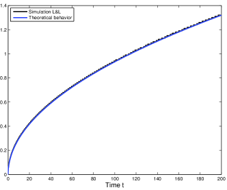
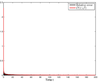
In the first example we compare the theoretical long time asymptotic behavior of the Lasry and Lions model (1) with the simulation results. Note that (1) corresponds to the simulation of (9) with b˙l(t)=b˙r(t)=0subscript˙𝑏𝑙𝑡subscript˙𝑏𝑟𝑡0\dot{b}_{l}(t)=\dot{b}_{r}(t)=0, that is the simulations of the heat equation with an initial datum of the form FI(x)=𝟙x<00.95×𝟙x>0subscript𝐹𝐼𝑥subscriptdouble-struck-𝟙𝑥00.95subscriptdouble-struck-𝟙𝑥0F_{I}(x)=\mathbb{1}_{x<0}-0.95\times\mathbb{1}_{x>0}. Figure 1 illustrates the behavior of the free boundary for the Lasry and Lions model (1) as a function of time. The relative error η=|ctpapprox(t)ct|𝜂𝑐𝑡subscript𝑝𝑎𝑝𝑝𝑟𝑜𝑥𝑡𝑐𝑡\eta=\lvert\frac{c\sqrt{t}-p_{approx}(t)}{c\sqrt{t}}\rvert decays fast in a good agreement of the numerically computed price papproxsubscript𝑝𝑎𝑝𝑝𝑟𝑜𝑥p_{approx} and the theoretical results. In fact the numerical results indicate that the relative error decays like t12superscript𝑡12t^{-\frac{1}{2}}, see Figure 1b).

Refer to caption
(a) Evolution of the price
Refer to caption
(b) Relative error η𝜂\eta
Figure 1. Comparison of the price evolution for the classic L&L model (1).

The next example illustrates the influence of the boundary on the price dynamics. Note that the stationary price psubscript𝑝p_{\infty} in the classic Lasry and Lions model on a bounded domain (pmax,pmax)subscript𝑝subscript𝑝(-p_{\max},p_{\max}) with Neumann boundary conditions is given by

p=2Mlpmaxa(MlMr)2(Ml+Mr)pmax2.subscript𝑝2superscript𝑀𝑙subscript𝑝𝑎superscript𝑀𝑙superscript𝑀𝑟2superscript𝑀𝑙superscript𝑀𝑟subscript𝑝2\displaystyle p_{\infty}=\frac{2M^{l}p_{\max}-a(M^{l}-M^{r})}{2(M^{l}+M^{r})}-\frac{p_{\max}}{2}. (34)

We choose an initial datum fIsubscript𝑓𝐼f_{I} with equal masses of buyers and vendors, i.e.

fI(x)={1 for 5x1x for 1<x22 for 2<x3.250 otherwise.subscript𝑓𝐼𝑥cases1 for 5𝑥1𝑥 for 1𝑥22 for 2𝑥3.250 otherwise.\displaystyle f_{I}(x)=\begin{cases}1&\text{ for }-5\leq x\leq-1\\ -x&\text{ for }-1<x\leq 2\\ 2&\text{ for }2<x\leq 3.25\\ 0&\text{ otherwise.}\end{cases}

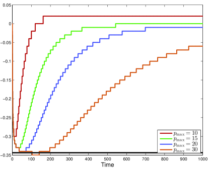
While the asymptotic analysis on the unbounded domain postulates the convergence towards the constant β2subscript𝛽2\beta_{2} given by (24), the stationary price on the bounded domain, given by (34), corresponds to p=0subscript𝑝0p_{\infty}=0. Figure 2 clearly illustrates the change of the price dynamics for differently sized domains Ω=[pmax,pmax]Ωsubscript𝑝subscript𝑝\Omega=[-p_{\max},p_{\max}]. The black line at p=0.3475𝑝0.3475p=-0.3475 corresponds to the predicted analytic constant - we observe that the prices initially converge to this value, but then reverse their dynamics towards p=0subscript𝑝0p_{\infty}=0 due to the influence of the boundary conditions. The smaller the computational domain the earlier the reversal happens.
Refer to caption
Figure 2. Evolution of the free boundary in the classic Lasry and Lions model in the case of equal market size distribution for different computational domains Ω=[pmax,pmax]Ωsubscript𝑝subscript𝑝\Omega=[-p_{\max},p_{\max}].

5.2. Price evolution for stabilizing market size fluctuations

Next we compare the simulated price dynamics for different choices of blsubscript𝑏𝑙b_{l} and brsubscript𝑏𝑟b_{r} with the theoretical results. We consider the three cases:

linear: bl(t)=cltt+1, exponential: bl(t)=cl(1exp(t2))quadratic: bl(t)=clt2t2+1,\displaystyle\begin{split}&\text{linear: }~{}b_{l}(t)=c_{l}\frac{t}{t+1},~{}\quad\text{ exponential: }b_{l}(t)=c_{l}(1-\exp(-t^{2}))\\ &\text{quadratic: }~{}b_{l}(t)=c_{l}\frac{t^{2}}{t^{2}+1},\end{split} (35)

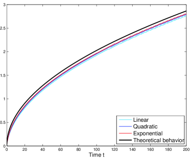
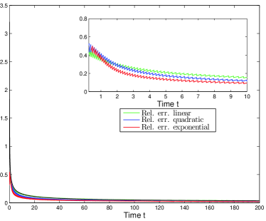
with cl=1.12345subscript𝑐𝑙1.12345c_{l}=1.12345. The fluctuations of the vendor market size distribution have the respectively same form with cr=1.0subscript𝑐𝑟1.0c_{r}=1.0. Hence bl=clsuperscriptsubscript𝑏𝑙subscript𝑐𝑙b_{l}^{\infty}=c_{l} and br=1superscriptsubscript𝑏𝑟1b_{r}^{\infty}=1. We start with simulations in the case of different initial masses of buyers and vendors. The initial datum is given by FI(x)=𝟙x<00.9×𝟙x>0subscript𝐹𝐼𝑥subscriptdouble-struck-𝟙𝑥00.9subscriptdouble-struck-𝟙𝑥0F_{I}(x)=\mathbb{1}_{x<0}-0.9\times\mathbb{1}_{x>0}. Figure 3 compares the theoretical long time asymptotics based on the results of Theorem 4.3 and the numerical simulations. We observe that the convergence rate of the functions blsubscript𝑏𝑙b_{l} and brsubscript𝑏𝑟b_{r} towards their asymptotic value determines the constant o(1)𝑜1o(1) - the faster the convergence the closer the behavior with respect to the theoretical predictions. The relative errors for the respective cases in Figure 3b) illustrate the fast convergence of the free boundary, they decay like t12superscript𝑡12t^{-\frac{1}{2}} (the inset in Figure 3(b) corresponds to the enlarged view of the price dynamics for small times).
Refer to caption
(a) Evolution of the price.
Refer to caption
(b) Relative error
Figure 3. Simulations in the case of deterministic fluctuations (35) with αlαrsuperscript𝛼𝑙superscript𝛼𝑟\alpha^{l}\neq\alpha^{r}.

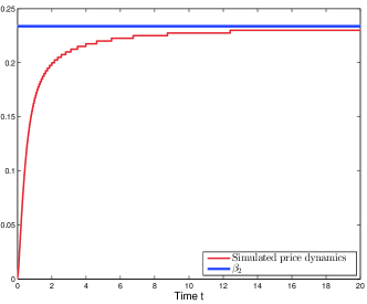
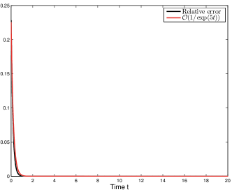
Next we consider the case αl=αrsuperscript𝛼𝑙superscript𝛼𝑟\alpha^{l}=\alpha^{r}, that is the number of buyers and vendors converge to the same long-time limit. Theorem 4.5 states that the long time asymptotic behavior is driven by the first order moments of the initial data. We choose the following initial datum:

FI(x)subscript𝐹𝐼𝑥\displaystyle F_{I}(x) ={40 if x<2,20x if 2x3,60 if x>3.absentcases40 if 𝑥220𝑥 if 2𝑥360 if 𝑥3\displaystyle=\begin{cases}40&\text{ if }x<-2,\\ -20x&\text{ if }-2\leq x\leq 3,\\ -60&\text{ if }x>3.\end{cases}

Furthermore we set

bl(t)=cl(1e5t) and br(t)=cr(1e5t)formulae-sequencesubscript𝑏𝑙𝑡subscript𝑐𝑙1superscript𝑒5𝑡 and subscript𝑏𝑟𝑡subscript𝑐𝑟1superscript𝑒5𝑡\displaystyle b_{l}(t)=c_{l}(1-e^{-5t})\quad\text{ and }\quad b_{r}(t)=c_{r}(1-e^{-5t})

with cl=log(1.1)+log(1.5)subscript𝑐𝑙1.11.5c_{l}=\log(1.1)+\log(1.5) and cr=log(1.1)subscript𝑐𝑟1.1c_{r}=\log(1.1). Note that the functions blsubscript𝑏𝑙b_{l} and brsubscript𝑏𝑟b_{r} satisfy Assumption A3(A3)(iv) and that the parameter choices imply αl=lMla=rMra=αrsuperscript𝛼𝑙superscript𝑙superscript𝑀𝑙𝑎superscript𝑟superscript𝑀𝑟𝑎superscript𝛼𝑟\alpha^{l}=\frac{l^{\infty}M^{l}}{a}=\frac{r^{\infty}M^{r}}{a}=\alpha^{r}. The evolution of the price is depicted in Figure 4. We observe the expected long time behavior towards the theoretically predicted constant β2subscript𝛽2\beta_{2}, but the decay is different. It decreases like exp5tsuperscript5𝑡\exp^{-5t}, illustrated in Figure 4b), and not like t12superscript𝑡12t^{-\frac{1}{2}} as in the case αlαrsuperscript𝛼𝑙superscript𝛼𝑟\alpha^{l}\neq\alpha^{r}.

Refer to caption
(a) Evolution of the price
Refer to caption
(b) Relative error
Figure 4. Simulations in the case of deterministic fluctuations (35) with αl=αrsuperscript𝛼𝑙superscript𝛼𝑟\alpha^{l}=\alpha^{r}.

5.3. Price evolution in the case of periodic market size fluctuations

Next we consider periodic fluctuations in the buyer and vendor market sizes. First we choose fluctuations of the form

bl(t)=cos(2πflt) and br(t)=cos(2πfrt).subscript𝑏𝑙𝑡2𝜋subscript𝑓𝑙𝑡 and subscript𝑏𝑟𝑡2𝜋subscript𝑓𝑟𝑡\displaystyle b_{l}(t)=\cos(2\pi f_{l}t)~{}~{}\text{ and }~{}~{}b_{r}(t)=\cos(2\pi f_{r}t). (36)

Figure 5 illustrates the behavior of the free boundary on the time interval t[0,1]𝑡01t\in[0,1] for different values of flsubscript𝑓𝑙f_{l} and frsubscript𝑓𝑟f_{r}, when the ratio fl\fr\subscript𝑓𝑙subscript𝑓𝑟f_{l}\backslash f_{r} is rational. We observe that the maximum amplitude of the computed price from the theoretical predictions decreases as ε0𝜀0\varepsilon\rightarrow 0, an observation also confirmed in Table 1.
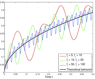
Refer to caption
Figure 5. Simulations in the case of periodic fluctuations (36) with zero mean.
flsubscript𝑓𝑙f_{l}/frsubscript𝑓𝑟f_{r} 5/10 10/20 20/40 50/100
amplitude 0.1389 0.1018 0.0777 0.0538
Table 1. Maximum deviation of the free boundary from the theoretical prediction due to periodic mass fluctuations of the form (36) in case of a rational fraction flfrsubscript𝑓𝑙subscript𝑓𝑟\frac{f_{l}}{f_{r}}.

Note that the functions bl=bl(t)subscript𝑏𝑙subscript𝑏𝑙𝑡b_{l}=b_{l}(t) and br=br(t)subscript𝑏𝑟subscript𝑏𝑟𝑡b_{r}=b_{r}(t) are one-periodic with zero mean in the first example and bl(0)=br(0)=1subscript𝑏𝑙0subscript𝑏𝑟01b_{l}(0)=b_{r}(0)=1. To illustrate the impact of mass fluctuations with non-zero mean we choose functions blsubscript𝑏𝑙b_{l} and brsubscript𝑏𝑟b_{r} of the form:

bl(t)=cos(πt)2 and br(t)=cos(2πt).\displaystyle b_{l}(t)=\cos(\pi t)^{2}~{}~{}\text{ and }~{}~{}b_{r}(t)=\cos(2\pi t). (37)

For this setting the corresponding evolution is illustrated in Figure 6 (using the same simulation parameters as in the previous example).
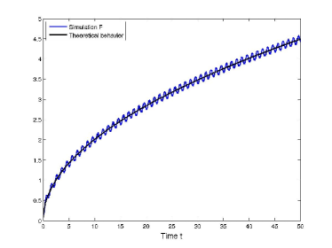
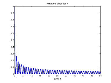
Refer to caption
(a) Evolution of the price
Refer to caption
(b) Relative error
Figure 6. Simulations in the case of periodic fluctuations (37) with non-zero mean.

Again we observe a very good agreement with the predicted theoretical price dynamics (based on the modified initial datum (33)), even though they are based on formal arguments.

Finally we study the effect of periodic mass fluctuations on the free boundary. We choose an initial datum with equal mass, that is FI(x)=𝟙x<0𝟙x>0subscript𝐹𝐼𝑥subscriptdouble-struck-𝟙𝑥0subscriptdouble-struck-𝟙𝑥0F_{I}(x)=\mathbb{1}_{x<0}-\mathbb{1}_{x>0} to clearly distinguish the influence of the market size fluctuations from the price dynamics due to the market imbalance of buyers and vendors. The functions blsubscript𝑏𝑙b_{l} and brsubscript𝑏𝑟b_{r} are set to

bl(t)=cos(πft)2 and br(t)=sin(2πft).\displaystyle b_{l}(t)=\cos(\pi ft)^{2}~{}~{}\text{ and }~{}~{}b_{r}(t)=\sin(2\pi ft). (38)

Table 2 states the computed amplitude and frequency for the different values of f𝑓f. Note that mass oscillations of order 𝒪(1)𝒪1\mathcal{O}(1) amplitude result in 𝒪(ε)𝒪𝜀\mathcal{O}(\varepsilon)-amplitude fluctuations in the free boundary and that we have ’numerical’ strong convergence of the free boundary.

f𝑓f 5 10 20 100
amplitude 0.1415 0.10446 0.075766 0.03982
frequency 4.8832 9.766 20.142 99.9456
Table 2. Frequency and amplitude of the price fluctuations for different values of f𝑓f.

5.4. Almost periodic market size fluctuations

We would like to argue numerically that the formal asymptotic for the periodic case, i.e. that the limiting dynamics of the price correspond to the dynamics of the original Lasry-Lions model with a changed initial buyer-vendor distribution (33), holds also in the case of Besicovitch almost periodic market size fluctuations, cf. [2]. Note that the space of Besicovitch almost periodic functions corresponds to the closure of the trigonometric polynomials under the seminorm

fB,p=lim supx(12xxx|f(s)|p𝑑s)1p.subscriptdelimited-∥∥𝑓𝐵𝑝subscriptlimit-supremum𝑥superscript12𝑥superscriptsubscript𝑥𝑥superscript𝑓𝑠𝑝differential-d𝑠1𝑝\displaystyle\lVert f\rVert_{B,p}=\limsup_{x\rightarrow\infty}\left(\frac{1}{2x}\int_{-x}^{x}\lvert f(s)\rvert^{p}ds\right)^{\frac{1}{p}}.

These functions have an expansion of the form naneiλntsubscript𝑛subscript𝑎𝑛superscript𝑒𝑖subscript𝜆𝑛𝑡\sum_{n}a_{n}e^{i\lambda_{n}t} with an2superscriptsubscript𝑎𝑛2\sum a_{n}^{2} finite and λnsubscript𝜆𝑛\lambda_{n}\in\mathbb{R}; their mean value is defined by

f:=limT1T0Tf(s)𝑑s.assigndelimited-⟨⟩𝑓subscript𝑇1𝑇superscriptsubscript0𝑇𝑓𝑠differential-d𝑠\displaystyle\langle f\rangle:=\lim_{T\rightarrow\infty}\frac{1}{T}\int_{0}^{T}f(s)ds. (39)

We set

bl(t)=sin(2πflt)+sin(2πflt(2)) and br(t)=cos(2πfrt)\displaystyle b_{l}(t)=\sin(2\pi f_{l}t)+\sin(2\pi f_{l}t\sqrt{(}2))\text{ and }b_{r}(t)=\cos(2\pi f_{r}t)

with integer frequencies flsubscript𝑓𝑙f_{l} and frsubscript𝑓𝑟f_{r} and choose an initial datum of the form FI(x)=𝟙x<012𝟙x0subscript𝐹𝐼𝑥subscriptdouble-struck-𝟙𝑥012subscriptdouble-struck-𝟙𝑥0F_{I}(x)=\mathbb{1}_{x<0}-\frac{1}{2}\mathbb{1}_{x\geq 0}. Figure 7 illustrates the price dynamics for the time interval t[0,1]𝑡01t\in[0,1] and the frequencies fl=fr=1,5,10,20,40formulae-sequencesubscript𝑓𝑙subscript𝑓𝑟15102040f_{l}=f_{r}=1,5,10,20,40. The black line corresponds to the theoretical prediction computed as in the periodic case, using the parameters bl=br=0delimited-⟨⟩subscript𝑏𝑙delimited-⟨⟩subscript𝑏𝑟0\langle b_{l}\rangle=\langle b_{r}\rangle=0, bl(0)=0subscript𝑏𝑙00b_{l}(0)=0 and br(0)=1subscript𝑏𝑟01b_{r}(0)=1. As already explained we observe convergence of the price towards the formal theoretical prediction in the periodic case, see (33). The numerical results indicate also the validity of the formal asymptotics in the almost periodic case.
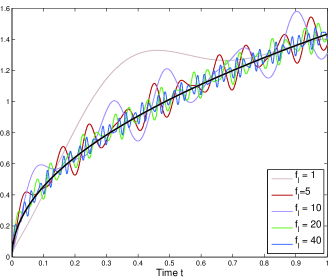
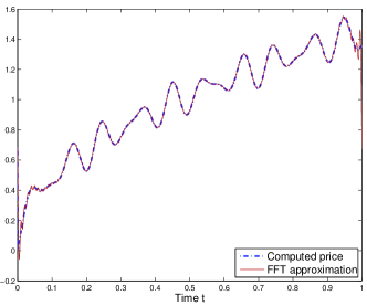
Refer to caption
(a) Price dynamics
Refer to caption
(b) Approximation of the price dynamics for fl=fr=10subscript𝑓𝑙subscript𝑓𝑟10f_{l}=f_{r}=10.
Figure 7. Price dynamics in case of almost-periodic market size fluctuations.

We would like to remark that it is difficult to determine if the discrete price dynamics are almost-periodic functions. Figure 7 shows the approximation of the price in the case fl=fr=10subscript𝑓𝑙subscript𝑓𝑟10f_{l}=f_{r}=10, which is based on the leading 100100100 FFT coefficients of the discrete price.

5.5. Price formation with stochastic market size fluctuations

Finally we consider the Lasry and Lions model (1) with stochastic fluctuations in the numbers of buyers and vendors, which we model by two independent Brownian motions Bl=Bl(t)subscript𝐵𝑙subscript𝐵𝑙𝑡B_{l}=B_{l}(t) and Br=Br(t)subscript𝐵𝑟subscript𝐵𝑟𝑡B_{r}=B_{r}(t) replacing the deterministic functions bl=bl(t)subscript𝑏𝑙subscript𝑏𝑙𝑡b_{l}=b_{l}(t) and br=br(t)subscript𝑏𝑟subscript𝑏𝑟𝑡b_{r}=b_{r}(t) in Section 3. Since under sufficient regularity conditions (such that Wong-Zakai type theorems for SPDEs hold, see  [26]) stochastic partial differential equations (SPDE) involving the Stratonovich integral are obtained in the limit (in probability) when Brownian motions are (reasonably) approximated by smooth functions. We shall use the Stratonovich version of the Lasry and Lions model following the common convention that Babsent𝐵\circ B denotes Stratonovich integration against B𝐵B.
Notice that the Stratonovich formulation is well defined when the Ito integral is well defined and the integrand is a semimartingale. In our case this can be guaranteed due to the special structure of the SPDE’s characteristics if sufficiently regular initial values are chosen. Also the Stratonovich correction term has a simple expression, since F|F|maps-to𝐹𝐹F\mapsto\lvert F\rvert and FFmaps-to𝐹𝐹F\mapsto F lead at least formally to the correction term 1/2F12𝐹1/2F. In the sequel we do not enter too much into the stochastic details but assume enough regularity for the initial values such that our considerations hold true.

Here we discuss the well posedness of the equation, but leave a more refined analysis, that is of long term limits, for future research. As a matter of fact we show that the influence of multiplicative stochastic market size fluctuations on the price evolution is relatively weak.

Using the same transformation (4) as in the beginning of Section 3 we obtain the stochastic equivalent of (10), in particular a heat equation with a multiplicative Lipschitz non-linearity in the stochastic term:

dF(x,t)=Fxx(x,t)dt+12F(x,t)(σldBl+σrdBr)+12|F(x,t)|(σldBlσrdBr).𝑑𝐹𝑥𝑡subscript𝐹𝑥𝑥𝑥𝑡𝑑𝑡12𝐹𝑥𝑡subscript𝜎𝑙𝑑subscript𝐵𝑙subscript𝜎𝑟𝑑subscript𝐵𝑟12𝐹𝑥𝑡subscript𝜎𝑙𝑑subscript𝐵𝑙subscript𝜎𝑟𝑑subscript𝐵𝑟\displaystyle\begin{split}dF(x,t)=F_{xx}(x,t)dt&+\frac{1}{2}F(x,t)\circ(\sigma_{l}dB_{l}+\sigma_{r}dB_{r}){}\\ &+\frac{1}{2}\lvert F(x,t)\rvert\circ(\sigma_{l}dB_{l}-\sigma_{r}dB_{r}).\end{split} (40)

We apply the transformation

V(x,t)=F(x,t)eσlBl+σrBr2,𝑉𝑥𝑡𝐹𝑥𝑡superscript𝑒subscript𝜎𝑙subscript𝐵𝑙subscript𝜎𝑟subscript𝐵𝑟2\displaystyle V(x,t)=F(x,t)e^{-\frac{\sigma_{l}B_{l}+\sigma_{r}B_{r}}{2}}, (41)

and obtain using the Stratonovich chain rule that

dV(x,t)=Vxx(x,t)+12|V(x,t)|(σldBlσrdBr).𝑑𝑉𝑥𝑡subscript𝑉𝑥𝑥𝑥𝑡12𝑉𝑥𝑡subscript𝜎𝑙𝑑subscript𝐵𝑙subscript𝜎𝑟𝑑subscript𝐵𝑟\displaystyle dV(x,t)=V_{xx}(x,t)+\frac{1}{2}\lvert V(x,t)\rvert\circ(\sigma_{l}dB_{l}-\sigma_{r}dB_{r}). (42)

The corresponding Ito equation is given by

dV(x,t)=Vxx(x,t)dt+σl2+σr28V(x,t)dt+12|V(x,t)|(σldBl+σrdBr).𝑑𝑉𝑥𝑡subscript𝑉𝑥𝑥𝑥𝑡𝑑𝑡superscriptsubscript𝜎𝑙2superscriptsubscript𝜎𝑟28𝑉𝑥𝑡𝑑𝑡12𝑉𝑥𝑡subscript𝜎𝑙𝑑subscript𝐵𝑙subscript𝜎𝑟𝑑subscript𝐵𝑟\displaystyle\begin{split}dV(x,t)=V_{xx}(x,t)dt&+\frac{\sigma_{l}^{2}+\sigma_{r}^{2}}{8}V(x,t)dt{}\\ &+\frac{1}{2}\lvert V(x,t)\rvert(\sigma_{l}dB_{l}+\sigma_{r}dB_{r}).\end{split} (43)

Another exponential transformation

U(x,t)=V(x,t)e(σl2+σr2)8t𝑈𝑥𝑡𝑉𝑥𝑡superscript𝑒superscriptsubscript𝜎𝑙2superscriptsubscript𝜎𝑟28𝑡\displaystyle U(x,t)=V(x,t)e^{-\frac{(\sigma_{l}^{2}+\sigma_{r}^{2})}{8}t}

yields, since Bl(0)=Br(0)=0subscript𝐵𝑙0subscript𝐵𝑟00B_{l}(0)=B_{r}(0)=0,

dU(x,t)=Uxx(x,t)dt+12|U(x,t)|(σldBlσrdBr) in ×+,𝑑𝑈𝑥𝑡subscript𝑈𝑥𝑥𝑥𝑡𝑑𝑡12𝑈𝑥𝑡subscript𝜎𝑙𝑑subscript𝐵𝑙subscript𝜎𝑟𝑑subscript𝐵𝑟 in subscript\displaystyle dU(x,t)=U_{xx}(x,t)dt+\frac{1}{2}\lvert U(x,t)\rvert(\sigma_{l}dB_{l}-\sigma_{r}dB_{r})\,\text{ in }\mathbb{R}\times\mathbb{R}_{+}, (44a)
U(x,t=0)=FI(x).𝑈𝑥𝑡0subscript𝐹𝐼𝑥\displaystyle U(x,t=0)=F_{I}(x). (44b)

This equation can be analyzed by the DaPrato-Zabczyk methodology (see [9]), which roughly speaking says that on every Hilbert space \mathcal{H} of real valued functions on \mathbb{R} where

  1. (1)

    the map F|F|𝐹𝐹F\rightarrow\lvert F\rvert is globally Lipschitz on \mathcal{H}, and

  2. (2)

    the one-dimensional Laplacian FFxxmaps-to𝐹subscript𝐹𝑥𝑥F\mapsto F_{xx} generates a strongly continuous semigroup S𝑆S (appropriately closed) on \mathcal{H},

there exists a unique mild solution of the SPDE. This process (U(t))t0subscript𝑈𝑡𝑡0{(U(t))}_{t\geq 0}, indexed in time t𝑡t and taking values in \mathcal{H}, satisfies, for every initial value F(0)𝐹0F(0)\in\mathcal{H}, the Duhamel formulation

U(t)=StU(0)+120tSts|U(s)|(σldBl(s)σrdBr(s)).𝑈𝑡subscript𝑆𝑡𝑈012superscriptsubscript0𝑡subscript𝑆𝑡𝑠𝑈𝑠subscript𝜎𝑙𝑑subscript𝐵𝑙𝑠subscript𝜎𝑟𝑑subscript𝐵𝑟𝑠\displaystyle\begin{split}U(t)=S_{t}U(0)+\frac{1}{2}\int_{0}^{t}S_{t-s}\lvert U(s)\rvert(\sigma_{l}dB_{l}(s)-\sigma_{r}dB_{r}(s)).\end{split} (45)

As usual we suppress the space (price) variable in this notation. The uniqueness of the solution of (44) is understood in the Banach space of cadlag processes with norm

UE[sup0sTU(s)2].maps-to𝑈𝐸delimited-[]subscriptsupremum0𝑠𝑇superscriptnorm𝑈𝑠2U\mapsto\sqrt{E\big{[}\sup_{0\leq s\leq T}{\|U(s)\|}^{2}\big{]}}\,.

Note that the form is not restricted to independent Brownian motions. In fact (45) can be solved for any two dimensional semi-martingale driving process (Sl,Sr)subscript𝑆𝑙subscript𝑆𝑟(S_{l},S_{r}), in particular also for Lévy processes; see Protter  [23] and, Peszat and Zabczyk [22] for more information.

From (45) we conclude that U𝑈U is given by the Feyman-Kac formula

U(x,t)=E[FI(x+2Wt)×exp(120tsign(U(x,s))(σldBl(s)σ2dBr(s)))].𝑈𝑥𝑡𝐸delimited-[]subscript𝐹𝐼𝑥2subscript𝑊𝑡12superscriptsubscript0𝑡sign𝑈𝑥𝑠subscript𝜎𝑙𝑑subscript𝐵𝑙𝑠subscript𝜎2𝑑subscript𝐵𝑟𝑠\displaystyle U(x,t)=E\Big{[}F_{I}(x+\sqrt{2}W_{t})\times\exp\big{(}\frac{1}{2}\int_{0}^{t}\operatorname{sign}(U(x,s))(\sigma_{l}dB_{l}(s)-\sigma_{2}dB_{r}(s))\big{)}\Big{]}.

This representation formula is justified by approximating the Brownian motions by piecewise constant interpolations and an application of the classical Feynman-Kac formula. Differentiating (45) with respect to x𝑥x, we find

Ux(t)=StUx(0)+120tStssign(U(s))Ux(s)(σldBl(s)σrdBr(s))t(σl2+σr2)/8.subscript𝑈𝑥𝑡subscript𝑆𝑡subscript𝑈𝑥012superscriptsubscript0𝑡subscript𝑆𝑡𝑠sign𝑈𝑠subscript𝑈𝑥𝑠subscript𝜎𝑙𝑑subscript𝐵𝑙𝑠subscript𝜎𝑟𝑑subscript𝐵𝑟𝑠𝑡superscriptsubscript𝜎𝑙2superscriptsubscript𝜎𝑟28\displaystyle\begin{split}U_{x}(t)=S_{t}U_{x}(0)+\frac{1}{2}\int_{0}^{t}S_{t-s}\operatorname{sign}\left(U(s)\right)U_{x}(s)\left(\sigma_{l}dB_{l}(s)-\sigma_{r}dB_{r}(s)\right)-t(\sigma_{l}^{2}+\sigma_{r}^{2})/8\,.\end{split} (46)

which then gives the Feynman-Kac representation namely

Ux(x,t)=E[FI,x(x+2Wt)×\displaystyle U_{x}(x,t)=E\Big{[}F_{I,x}(x+\sqrt{2}W_{t})\times
×exp(120t(sign(U(x+2Ws,s))σldBl(s)sign(U(x+2Ws,s))σrdBr(s))t(σl2+σr2)/8)]\displaystyle\quad\times\exp\big{(}\frac{1}{2}\int_{0}^{t}(\operatorname{sign}(U(x+\sqrt{2}W_{s},s))\sigma_{l}dB_{l}(s)-\operatorname{sign}(U(x+\sqrt{2}W_{s},s))\sigma_{r}dB_{r}(s))-t(\sigma_{l}^{2}+\sigma_{r}^{2})/8\big{)}\Big{]}\,

It is an easy consequence of this representation that for monotonically decreasing non-constant initial data FIsubscript𝐹𝐼F_{I} positivity of Ux(t)subscript𝑈𝑥𝑡U_{x}(t) holds instantaneously for t>0𝑡0t>0. This implies that, for such initial data, there exists at most one zero x=p(t)𝑥𝑝𝑡x=p(t) of U(t)𝑈𝑡U(t) for every t>0𝑡0t>0, that is the free boundary cannot turn back or develop fat parts in finite time. By smoothing the Brownian processes Blsubscript𝐵𝑙B_{l} and Brsubscript𝐵𝑟B_{r} in (44) we conclude for general initial data FIsubscript𝐹𝐼F_{I} that the zero level set of the solution U𝑈U is the graph limit of a sequence of functions of time. This excludes in particular that the free boundary can turn back but it does not exclude the formation of fat parts.

Although the main focus of this paper was the long time behavior of the free boundary we conclude with a short heuristic calculation which illustrates why we cannot expect very volatile dynamics in the case of Brownian drivers: we consider an (exponential) Euler step for a short period of time denoted by t>0𝑡0t>0. Let S𝑆S denote the heat semigroup and E0,tsubscript𝐸0𝑡E_{0,t} the random operator defined for xp(t)𝑥𝑝𝑡x\leq p(t) by

E0,tU(x):=U(x)exp(σlBl(t)σl2t2),assignsubscript𝐸0𝑡𝑈𝑥𝑈𝑥subscript𝜎𝑙subscript𝐵𝑙𝑡superscriptsubscript𝜎𝑙2𝑡2\displaystyle E_{0,t}U(x):=U(x)\exp\big{(}\sigma_{l}B_{l}(t)-\frac{\sigma_{l}^{2}t}{2}\big{)}, (47a)
and for xp(t)𝑥𝑝𝑡x\geq p(t) by
E0,tU(x):=U(x)exp(σrBr(t)σr2t2).assignsubscript𝐸0𝑡𝑈𝑥𝑈𝑥subscript𝜎𝑟subscript𝐵𝑟𝑡superscriptsubscript𝜎𝑟2𝑡2\displaystyle E_{0,t}U(x):=U(x)\exp\big{(}\sigma_{r}B_{r}(t)-\frac{\sigma_{r}^{2}t}{2}\big{)}. (47b)

We evaluate the concatenation of these operators for a C1superscript𝐶1C^{1} function U𝑈U with precisely one zero at p𝑝p with U(p)<0superscript𝑈𝑝0U^{\prime}(p)<0 for small times t𝑡t and for x𝑥x close to p𝑝p. We have

StE0,tU(x)=ϕ(y)(\displaystyle S_{t}E_{0,t}U(x)=\int_{-\infty}^{\infty}\phi(y)\big{(} 1{x+2typ}κlU(p)(x+2typ)+limit-fromsubscript1𝑥2𝑡𝑦𝑝subscript𝜅𝑙superscript𝑈𝑝𝑥2𝑡𝑦𝑝\displaystyle 1_{\{x+\sqrt{2t}y\leq p\}}\kappa_{l}U^{\prime}(p)(x+\sqrt{2t}y-p)+
+\displaystyle+ 1{x+2typ}κrU(p)(x+2typ))dy,\displaystyle 1_{\{x+\sqrt{2t}y\geq p\}}\kappa_{r}U^{\prime}(p)(x+\sqrt{2t}y-p)\big{)}dy\,,

where ϕitalic-ϕ\phi is the standard normal density and

κl/r=κl/r(t)=exp(σl/rBl/r(t)σl/r2t2).subscript𝜅𝑙𝑟subscript𝜅𝑙𝑟𝑡subscript𝜎𝑙𝑟subscript𝐵𝑙𝑟𝑡superscriptsubscript𝜎𝑙𝑟2𝑡2\kappa_{l/r}=\kappa_{l/r}(t)=\exp\big{(}\sigma_{l/r}B_{l/r}(t)-\frac{\sigma_{l/r}^{2}t}{2}\big{)}\,.

For small times t𝑡t we obtain

StE0,tU(x)subscript𝑆𝑡subscript𝐸0𝑡𝑈𝑥\displaystyle S_{t}E_{0,t}U(x) =U(p)κl(xp)Φ(xp)+U(p)κr(xp)(1Φ(xp))absentsuperscript𝑈𝑝subscript𝜅𝑙𝑥𝑝Φ𝑥𝑝superscript𝑈𝑝subscript𝜅𝑟𝑥𝑝1Φ𝑥𝑝\displaystyle=U^{\prime}(p)\kappa_{l}(x-p)\Phi(x-p)+U^{\prime}(p)\kappa_{r}(x-p)(1-\Phi(x-p))
+U(p)(κl+κr)2tϕ(xp),superscript𝑈𝑝subscript𝜅𝑙subscript𝜅𝑟2𝑡italic-ϕ𝑥𝑝\displaystyle+U^{\prime}(p)(-\kappa_{l}+\kappa_{r})\sqrt{2t}\phi(x-p)\,,

which implies that for small times p(t)𝑝𝑡p(t) is of the form:

p(t)p+2(κrκl)π(κr+κl)t+𝒪(t).𝑝𝑡𝑝2subscript𝜅𝑟subscript𝜅𝑙𝜋subscript𝜅𝑟subscript𝜅𝑙𝑡𝒪𝑡\displaystyle p(t)\approx p+\frac{2(\kappa_{r}-\kappa_{l})}{\sqrt{\pi}(\kappa_{r}+\kappa_{l})}\sqrt{t}+\mathcal{O}(t)\,. (48)

This formula implies that we do actually observe t𝑡\sqrt{t} asymptotics weighted with factors stemming from κrκlsubscript𝜅𝑟subscript𝜅𝑙\kappa_{r}-\kappa_{l} for small times as well. The asymptotics are also of order of magnitude t𝑡\sqrt{t} due to the Brownian increments in the exponent. This implies that the increments of the price process p(t)p(0)𝑝𝑡𝑝0p(t)-p(0) are 𝒪(t)𝒪𝑡\mathcal{O}(t) even in the presence of Brownian drivers, and therefore of finite total variation for tp(t)maps-to𝑡𝑝𝑡t\mapsto p(t). Hence the price process does not admit a martingale part, which implies that even proportional fluctuations of buyers and vendors densities by independent Brownian motions do not lead to price curves as observed in realistic markets.
On the other hand the short time asymptotics give a hint how to introduce “more” randomness to obtain a martingale price process p𝑝p. This is that the densities of the buyer and vendor must be perturbed on small intervals of length t𝑡t by multiplicative noises of 𝒪(1)𝒪1\mathcal{O}(1). This, however, does not lead to the type of SPDE (45) originally proposed in this section.

Numerical simulations

In the first example we would like to confirm the small time asymptotic behavior of the free boundary p(t)𝑝𝑡p(t) given by (48). We start with an initial datum of the form

FI(x)=x,subscript𝐹𝐼𝑥𝑥\displaystyle F_{I}(x)=-x,

and set σr=σl=1subscript𝜎𝑟subscript𝜎𝑙1\sigma_{r}=\sigma_{l}=1. We use the domain ΩΩ\Omega to [10,10]1010[-10,10] and run the simulation on the time interval t[0,1]𝑡01t\in[0,1]. The spatial discretization corresponds to equidistant intervals of size h=103superscript103h=10^{-3}, while the time steps are set to Δt=105Δ𝑡superscript105\Delta t=10^{-5}. At time t=0.5𝑡0.5t=0.5 we choose two independent normally distributed random numbers ΔB1Δsuperscript𝐵1\Delta B^{1}, ΔB2Δsuperscript𝐵2\Delta B^{2} with standard deviation ΔtΔ𝑡\sqrt{\Delta t} and multiply the distribution left of the price with exp(ΔB1Δt/2)Δsuperscript𝐵1Δ𝑡2\exp(\Delta B^{1}-\Delta t/2) and the right of the price with exp(ΔB2Δt/2)Δsuperscript𝐵2Δ𝑡2\exp(\Delta B^{2}-\Delta t/2). Figure 8 illustrates the small time asymptotics - the initial price up to time t=0.5𝑡0.5t=0.5 equals to zero due to the same total number of buyers and vendors. Then the stochastic fluctuations in the buyer and vendor density initiate a new price dynamic, which confirms the estimated behavior given by (48).
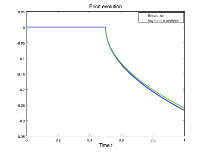
Refer to caption
Figure 8. Short-time asymptotics in case of stochastic market size fluctuations

We conclude with an example illustrating the necessity to add “more” randomness to the model. We start with an initial datum of the form FI(x)=𝟙x<0𝟙x>0subscript𝐹𝐼𝑥subscriptdouble-struck-𝟙𝑥0subscriptdouble-struck-𝟙𝑥0F_{I}(x)=\mathbb{1}_{x<0}-\mathbb{1}_{x>0} and time steps of Δt=105Δ𝑡superscript105\Delta t=10^{-5}. At time t=0.25,0.5𝑡0.250.5t=0.25,~{}0.5 and t=0.75𝑡0.75t=0.75 we multiply the right and left distribution by two independent normally distributed random numbers ΔB1Δsuperscript𝐵1\Delta B^{1} and ΔB2Δsuperscript𝐵2\Delta B^{2} with standard deviation ΔtslowΔsubscript𝑡𝑠𝑙𝑜𝑤\sqrt{\Delta t_{slow}}, where ΔtslowΔsubscript𝑡𝑠𝑙𝑜𝑤\Delta t_{slow} denotes the slow time scale, that is Δtslow=0.25Δsubscript𝑡𝑠𝑙𝑜𝑤0.25\Delta t_{slow}=0.25. The corresponding price dynamics are depicted in Figure 9, which depicts a sequence of square-root like curves. Each one evolves according to the estimated behavior discussed in this subsection.
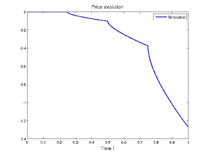
Refer to caption
Figure 9. Price evolution under ’slow scale’ market size fluctuations

Acknowledgment

We are grateful to Panagiotis Souganidis for generously sharing his ideas with us during the course of this research and for helpinng us substantially in improving the presentation.

MTW acknowledges financial support from the Austrian Academy of Sciences ÖAW via the New Frontiers Group NFG-001. PES was partially supported by the NSF.

References

  • [1] S. Angenent. The zero set of a solution of a parabolic equation. J. Reine Angew. Math, 390:79–96, 1988.
  • [2] A. S. Besicovitch. Almost periodic functions. Dover Publications, Inc., New York, 1955.
  • [3] M. Burger, L. Caffarelli, P. Markowich, and M.-T. Wolfram. On a Boltzmann-type price formation model. Proc. R. Soc. A, 469(2157), 2013.
  • [4] M. Burger, L. Caffarelli, P. A. Markowich, and M.-T. Wolfram. On the asymptotic behavior of a Boltzmann-type price formation model. Commun. Math. Sci., 12(7):1353–1361, 2014.
  • [5] M. Burger, A. Lorz, and M.T. Wolfram. On a Boltzmann mean field model for knowledge growth. Technical report, arxiv, submitted, 2015.
  • [6] L. A. Caffarelli, P. A. Markowich, and J.-F. Pietschmann. On a price formation free boundary model by Lasry and Lions. C. R. Math. Acad. Sci. Paris, 349(11-12):621–624, 2011.
  • [7] L. A. Caffarelli, P. A. Markowich, and M.-T. Wolfram. On a price formation free boundary model by Lasry and Lions: the Neumann problem. C. R. Math. Acad. Sci. Paris, 349(15-16):841–844, 2011.
  • [8] L. Chayes, M. del Mar González, M. P. Gualdani, and I. Kim. Global existence and uniqueness of solutions to a model of price formation. SIAM J. Math. Anal., 41(5):2107–2135, 2009.
  • [9] G. Da Prato and J. Zabczyk. Stochastic equations in infinite dimensions, volume 152 of Encyclopedia of Mathematics and its Applications. Cambridge University Press, Cambridge, second edition, 2014.
  • [10] P. Degond, J.-G. Liu, and C. Ringhofer. Evolution of wealth in a non-conservative economy driven by local Nash equilibria. Philosophical Transactions of the Royal Society of London A: Mathematical, Physical and Engineering Sciences, 372(2028), 2014.
  • [11] P. Degond, J.-G. Liu, and C. Ringhofer. Large-scale dynamics of mean-field games driven by local Nash equilibria. Journal of Nonlinear Science, 24(1):93–115, 2014.
  • [12] B. Düring and G. Toscani. Hydrodynamics from kinetic models of conservative economies. Physica A: Statistical Mechanics and its Applications, 384(2):493–506, 2007.
  • [13] E. Faou. Analysis of splitting methods for reaction-diffusion problems using stochastic calculus. Mathematics of Computation, 78(267):1467–1483, 2009.
  • [14] V. A. Galaktionov. Geometric Sturmian theory of nonlinear parabolic equations and applications. Chapman & Hall/CRC Applied Mathematics and Nonlinear Science Series, 3. Chapman & Hall/CRC, Boca Raton, FL, 2004.
  • [15] M. del Mar González and M. P. Gualdani. Asymptotics for a symmetric equation in price formation. Appl. Math. Optim., 59(2):233–246, 2009.
  • [16] A. Lachapelle, J.M. Lasry, C.A. Lehalle, and P.-L. Lions. Efficiency of the price formation process in presence of high frequency participants: a mean field game analysis. arXiv preprint arXiv:1305.6323, 2013.
  • [17] J.M. Lasry and P.-L. Lions. Mean field games. Jpn. J. Math., 2(1):229–260, 2007.
  • [18] P. A. Markowich, N. Matevosyan, J.-F. Pietschmann, and M.-T. Wolfram. On a parabolic free boundary equation modeling price formation. Math. Models Methods Appl. Sci., 19(10):1929–1957, 2009.
  • [19] M. O’Hara. Market microstructure theory, volume 108. Blackwell Cambridge, MA, 1995.
  • [20] L. Pareschi and G. Toscani. Interacting Multiagent Systems: Kinetic equations and Monte Carlo methods. OUP Oxford, 2013.
  • [21] L. Pareschi and G. Toscani. Wealth distribution and collective knowledge: a Boltzmann approach. Philosophical Transactions of the Royal Society A: Mathematical, Physical and Engineering Sciences, 372(2028):20130396, 2014.
  • [22] S. Peszat and J. Zabczyk. Stochastic partial differential equations with Lévy noise, volume 113 of Encyclopedia of Mathematics and its Applications. Cambridge University Press, Cambridge, 2007. An evolution equation approach.
  • [23] P. E. Protter. Stochastic integration and differential equations, volume 21 of Stochastic Modelling and Applied Probability. Springer-Verlag, Berlin, 2005. Second edition. Version 2.1, Corrected third printing.
  • [24] G. Toscani. Kinetic models of opinion formation. Communications in Mathematical Sciences, 4(3):481–496, 2006.
  • [25] G. Toscani, C. Brugna, and S. Demichelis. Kinetic models for the trading of goods. Journal of Statistical Physics, 151(3-4):549–566, 2013.
  • [26] N. Toshiyuki. Support theorem for mild solutions of SDE’s in Hilbert spaces. J. Math. Sci. Univ. Tokyo, 11(3):245–311, 2004.