Revisiting Batch Normalization For
Practical Domain Adaptation
Abstract
Deep neural networks (DNN) have shown unprecedented success in various computer vision applications such as image classification and object detection. However, it is still a common annoyance during the training phase, that one has to prepare at least thousands of labeled images to fine-tune a network to a specific domain. Recent study (Tommasi et al., 2015) shows that a DNN has strong dependency towards the training dataset, and the learned features cannot be easily transferred to a different but relevant task without fine-tuning. In this paper, we propose a simple yet powerful remedy, called Adaptive Batch Normalization (AdaBN) to increase the generalization ability of a DNN. By modulating the statistics in all Batch Normalization layers across the network, our approach achieves deep adaptation effect for domain adaptation tasks. In contrary to other deep learning domain adaptation methods, our method does not require additional components, and is parameter-free. It archives state-of-the-art performance despite its surprising simplicity. Furthermore, we demonstrate that our method is complementary with other existing methods. Combining AdaBN with existing domain adaptation treatments may further improve model performance.
1 Introduction
Training a DNN for a new image recognition task is expensive. It requires a large amount of labeled training images that are not easy to obtain. One common practice is to use labeled data from other related source such as a different public dataset, or harvesting images by keywords from a search engine. Because 1) the distributions of the source domains (third party datasets or Internet images) are often different from the target domain (testing images); and 2) DNN is particularly good at capturing dataset bias in its internal representation (Torralba & Efros, 2011), which eventually leads to overfitting, imperfectly paired training and testing sets usually leads to inferior performance.
Known as domain adaptation, the effort to bridge the gap between training and testing data distributions has been discussed several times under the context of deep learning (Tzeng et al., 2014; Long et al., 2015; Tzeng et al., 2015; Ganin & Lempitsky, 2015). To make the connection between the domain of training and the domain of testing, most of these methods require additional optimization steps and extra parameters. Such additional computational burden could greatly complicate the training of a DNN which is already intimidating enough for most people.
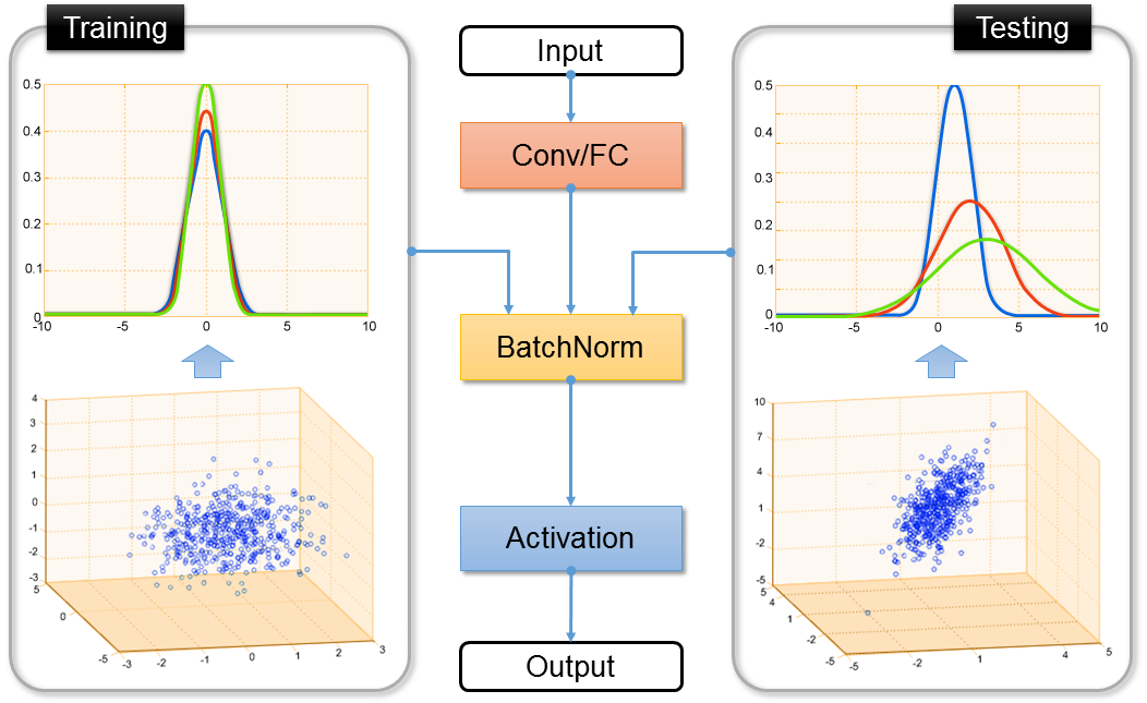
In this paper, we propose a simple yet effective approach called AdaBN for batch normalized DNN domain adaptation. We hypothesize that the label related knowledge is stored in the weight matrix of each layer, whereas domain related knowledge is represented by the statistics of the Batch Normalization (BN) (Ioffe & Szegedy, 2015) layer. Therefore, we can easily transfer the trained model to a new domain by modulating the statistics in the BN layer. This approach is straightforward to implement, has zero parameter to tune, and requires minimal computational resources. Moreover, our AdaBN is ready to be extended to more sophisticated scenarios such as multi-source domain adaptation and semi-supervised settings. Fig. 1 illustrates the flowchart of AdaBN. To summarize, our contributions are as follows:
-
1.
We propose a novel domain adaptation technique called Adaptive Batch Normalization (AdaBN). We show that AdaBN can naturally dissociate bias and variance of a dataset, which is ideal for domain adaptation tasks.
-
2.
We validate the effectiveness of our approach on standard benchmarks for both single source and multi-source domain adaptation. Our method outperforms the state-of-the-art methods.
-
3.
We conduct experiments on the cloud detection for remote sensing images to further demonstrate the effectiveness of our approach in practical use.
2 Related Work
Domain transfer in visual recognition tasks has gained increasing attention in recent literature (Beijbom, 2012; Patel et al., 2015). Often referred to as covariate shift (Shimodaira, 2000) or dataset bias (Torralba & Efros, 2011), this problem poses a great challenge to the generalization ability of a learned model. One key component of domain transfer is to model the difference between source and target distributions. In Khosla et al. (2012), the authors assign each dataset with an explicit bias vector, and train one discriminative model to handle multiple classification problems with different bias terms. A more explicit way to compute dataset difference is based on Maximum Mean Discrepancy (MMD) (Gretton et al., 2012). This approach projects each data sample into a Reproducing Kernel Hilbert Space, and then computes the difference of sample means. To reduce dataset discrepancies, many methods are proposed, including sample selections (Huang et al., 2006; Gong et al., 2013), explicit projection learning (Pan et al., 2011; Gopalan et al., 2011; Baktashmotlagh et al., 2013) and principal axes alignment (Fernando et al., 2013; Gong et al., 2012; Aljundi et al., 2015).
All of these methods face the same challenge of constructing the domain transfer function – a high-dimensional non-linear function. Due to computational constraints, most of the proposed transfer functions are in the category of simple shallow projections, which are typically composed of kernel transformations and linear mapping functions.
In the field of deep learning, feature transferability across different domains is a tantalizing yet generally unsolved topic (Yosinski et al., 2014; Tommasi et al., 2015). To transfer the learned representations to a new dataset, pre-training plus fine-tuning (Donahue et al., 2014) have become de facto procedures. However, adaptation by fine-tuning is far from perfect. It requires a considerable amount of labeled data from the target domain, and non-negligible computational resources to re-train the whole network.
A series of progress has been made in DNN to facilitate domain transfer. Early works of domain adaptation either focus on reordering fine-tuning samples (Chopra et al., 2013), or regularizing MMD (Gretton et al., 2012) in a shallow network (Ghifary et al., 2014). It is only until recently that the problem is directly attacked under the setting of classification of unlabeled target domain using modern convolutional neural network (CNN) architecture. DDC (Tzeng et al., 2014) used the classical MMD loss to regularize the representation in the last layer of CNN. DAN (Long et al., 2015) further extended the method to multiple kernel MMD and multiple layer adaptation. Besides adapting features using MMD, RTN (Long et al., 2016) also added a gated residual layer for classifier adaptation. RevGrad (Ganin & Lempitsky, 2015) devised a gradient reversal layer to compensate the back-propagated gradients that are domain specific. Recently, by explicitly modeling both private and shared components of the domain representations in the network, Bousmalis et al. (2016) proposed a Domain Separation Network to extract better domain-invariant features.
Another related work is CORAL (Sun et al., 2016). This model focuses on the last layer of CNN. CORAL whitens the data in source domain, and then re-correlates the source domain features to target domain. This operation aligns the second order statistics of source domain and target domain distributions. Surprisingly, such simple approach yields state-of-the-arts results in various text classification and visual recognition tasks. Recently, Deep CORAL (Sun & Saenko, 2016) also extends the method into DNN by incorporating a CORAL loss.
2.1 Batch Normalization
In this section, we briefly review Batch Normalization (BN) (Ioffe & Szegedy, 2015) which is closely related to our AdaBN. The BN layer is originally designed to alleviate the issue of internal covariate shifting – a common problem while training a very deep neural network. It first standardizes each feature in a mini-batch, and then learns a common slope and bias for each mini-batch. Formally, given the input to a BN layer , where denotes the batch size, and is the feature dimension, BN layer transforms a feature into:
| (1) | ||||
where and are the input/output scalars of one neuron response in one data sample; denotes the column of the input data; and and are parameters to be learned. This transformation guarantees that the input distribution of each layer remains unchanged across different mini-batches. For Stochastic Gradient Descent (SGD) optimization, a stable input distribution could greatly facilitate model convergence, leading to much faster training speed for CNN. Moreover, if training data are shuffled at each epoch, the same training sample will be applied with different transformations, or in other words, more comprehensively augmented throughout the training. During the testing phase, the global statistics of all training samples is used to normalize every mini-batch of test data.
Extensive experiments have shown that Batch Normalization significantly reduces the number of iteration to converge, and improves the final performance at the same time. BN layer has become a standard component in recent top-performing CNN architectures, such as deep residual network (He et al., 2016), and Inception V3 (Szegedy et al., 2015).
3 The Model
In Sec. 3.1, we first analyze the domain shift in deep neural network, and reveal two key observations. Then in Sec. 3.2, we introduce our Adaptive Batch Normalization (AdaBN) method based on these observations. Finally, we analyze our method in-depth in Sec. 3.3.
3.1 A Pilot Experiment
Although the Batch Normalization (BN) technique is originally proposed to help SGD optimization, its core idea is to align the distribution of training data. From this perspective, it is interesting to examine the BN parameters (batch-wise mean and variance) over different dataset at different layers of the network.
In this pilot experiment, we use MXNet implementation (Chen et al., 2016b) of the Inception-BN model (Ioffe & Szegedy, 2015) pre-trained on ImageNet classification task (Russakovsky et al., 2015) as our baseline DNN model. Our image data are drawn from (Bergamo & Torresani, 2010), which contains the same classes of images from both Caltech-256 dataset (Griffin et al., 2007) and Bing image search results. For each mini-batch sampled from one dataset, we concatenate the mean and variance of all neurons from one layer to form a feature vector. Using linear SVM, we can almost perfectly classify whether the mini-batch feature vector is from Caltech-256 or Bing dataset. Fig. 2 visualizes the distributions of mini-batch feature vectors from two datasets in 2D. It is clear that BN statistics from different domains are separated into clusters.
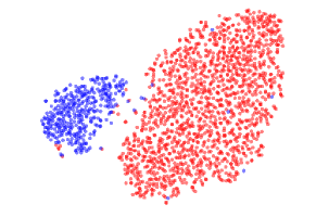
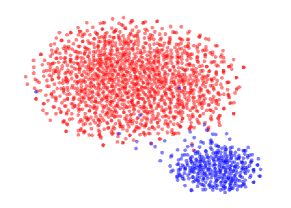
This pilot experiment suggests:
-
1.
Both shallow layers and deep layers of the DNN are influenced by domain shift. Domain adaptation by manipulating the output layer alone is not enough.
-
2.
The statistics of BN layer contain the traits of the data domain.
Both observations motivate us to adapt the representation across different domains by BN layer.
3.2 Adaptive Batch Normalization
Given the pre-trained DNN model and a target domain, our Adaptive Batch Normalization algorithm is as follows111In practice we adopt an online algorithm (Donald, 1999) to efficiently estimate the mean and variance.:
The intuition behind our method is straightforward: The standardization of each layer by domain ensures that each layer receives data from a similar distribution, no matter it comes from the source domain or the target domain.
For domain adaptation where , we standardize each sample by the statistics in its own domain. During training, the statistics are calculated for every mini-batch, the only thing that we need to make sure is that the samples in every mini-batch are from the same domain.
For (semi-)supervised domain adaptation, we may use the labeled data to fine-tune the weights as well. As a result, our method could fit in all different settings of domain adaptation with minimal effort.
3.3 Further Thoughts About Adabn
The simplicity of AdaBN is in sharp contrast to the complication of the domain shift problem. One natural question to ask is whether such simple translation and scaling operations could approximate the intrinsically non-linear domain transfer function.
Consider a simple neural network with input . It has one BN layer with mean and variance of each feature being and (), one fully connected layer with weight matrix and bias , and a non-linear transformation layer , where and correspond to the input and output feature size. The output of this network is , where
| (2) | ||||||
The output without BN is simply . We can see that the transformation is highly non-linear even for a simple network with one computation layer. As CNN architecture goes deeper, it will gain increasing power to represent more complicated transformations.
Another question is why we transform the neuron responses independently, not decorrelate and then re-correlate the responses as suggested in Sun et al. (2016). Under certain conditions, decorrelation could improve the performance. However, in CNN, the mini-batch size is usually smaller than the feature dimension, leading to singular covariance matrices that is hard to be inversed. As a result, the covariance matrix is always singular. In addition, decorrelation requires to compute the inverse of the covariance matrix which is computationally intensive, especially if we plan to apply AdaBN to all layers of the network.
4 Experiments
In this section, we demonstrate the effectiveness of AdaBN on standard domain adaptation datasets, and empirically analyze the adapted features. We also evaluation our method on a practical application with remote sensing images.
4.1 Experimental Settings
We first introduce our experiments on two standard datasets: Office (Saenko et al., 2010) and Caltech-Bing (Bergamo & Torresani, 2010).
Office (Saenko et al., 2010) is a standard benchmark for domain adaptation, which is a collection of 4652 images in 31 classes from three different domains: Amazon(A), DSRL(D) and Webcam(W). Similar to (Tzeng et al., 2014; Sun et al., 2016; Long et al., 2015), we evaluate the pairwise domain adaption performance of AdaBN on all six pairs of domains. For the multi-source setting, we evaluate our method on three transfer tasks {A, W} D, {A, D} W, {D, W} A.
Caltech-Bing (Bergamo & Torresani, 2010) is a much larger domain adaptation dataset, which contains 30,607 and 121,730 images in 256 categories from two domains Caltech-256(C) and Bing(B). The images in the Bing set are collected from Bing image search engine by keyword search. Apparently Bing data contains noise, and its data distribution is dramatically different from that of Caltech-256.
We compare our approach with a variety of methods, including four shallow methods: SA (Fernando et al., 2013), LSSA (Aljundi et al., 2015), GFK (Gong et al., 2012), CORAL (Sun et al., 2016), and four deep methods: DDC (Tzeng et al., 2014), DAN (Long et al., 2015), RevGrad (Ganin & Lempitsky, 2015), Deep CORAL (Sun & Saenko, 2016). Specifically, GFK models domain shift by integrating an infinite number of subspaces that characterize changes in statistical properties from the source to the target domain. SA, LSSA and CORAL align the source and target subspaces by explicit feature space transformations that would map source distribution into the target one. DDC and DAN are deep learning based methods which maximize domain invariance by adding to AlexNet one or several adaptation layers using MMD. RevGrad incorporates a gradient reversal layer in the deep model to encourage learning domain-invariant features. Deep CORAL extends CORAL to perform end-to-end adaptation in DNN. It should be noted that these deep learning methods have the adaptation layers on top of the output layers of DNNs, which is a sharp contrast to our method that delves into early convolution layers as well with the help of BN layers.
We follow the full protocol (Donahue et al., 2014) for the single source setting; while for multiple sources setting, we use all the samples in the source domains as training data, and use all the samples in the target domain as testing data. We fine-tune the Inception-BN (Ioffe & Szegedy, 2015) model on source domain in each task for 100 epochs. The learning rate is set to initially, and then is dropped by a factor every 40 epochs. Since the office dataset is quite small, following the best practice in Long et al. (2015), we freeze the first three groups of Inception modules, and set the learning rate of fourth and fifth group one tenth of the base learning rate to avoid overfitting. For Caltech-Bing dataset, we fine-tune the whole model with the same base learning rate.
4.2 Results
4.2.1 Office Dataset
Our results on Office dataset is reported in Table 1 and Table 2 for single/multi source(s), respectively. Note that the first 5 models of the Table 1 are pre-trained on AlexNet (Krizhevsky et al., 2012) instead of the Inception-BN (Ioffe & Szegedy, 2015) model, due to the lack of publicly available pre-trained Inception BN model in Caffe (Jia et al., 2014). Thus, the relative improvements over the baseline (AlexNet/Inception BN) make more sense than the absolute numbers of each algorithm.
| Method | A W | D W | W D | A D | D A | W A | Avg |
|---|---|---|---|---|---|---|---|
| AlexNet (Krizhevsky et al., 2012) | 61.6 | 95.4 | 99.0 | 63.8 | 51.1 | 49.8 | 70.1 |
| DDC (Tzeng et al., 2014) | 61.8 | 95.0 | 98.5 | 64.4 | 52.1 | 52.2 | 70.6 |
| DAN (Long et al., 2015) | 68.5 | 96.0 | 99.0 | 67.0 | 54.0 | 53.1 | 72.9 |
| Deep CORAL (Sun & Saenko, 2016) | 66.4 | 95.7 | 99.2 | 66.8 | 52.8 | 51.5 | 72.1 |
| RevGrad (Ganin & Lempitsky, 2015) | 67.3 | 94.0 | 93.7 | - | - | - | - |
| Inception BN (Ioffe & Szegedy, 2015) | 70.3 | 94.3 | 100 | 70.5 | 60.1 | 57.9 | 75.5 |
| SA (Fernando et al., 2013) | 69.8 | 95.5 | 99.0 | 71.3 | 59.4 | 56.9 | 75.3 |
| GFK (Gong et al., 2012) | 66.7 | 97.0 | 99.4 | 70.1 | 58.0 | 56.9 | 74.7 |
| LSSA (Aljundi et al., 2015) | 67.7 | 96.1 | 98.4 | 71.3 | 57.8 | 57.8 | 74.9 |
| CORAL (Sun et al., 2016) | 70.9 | 95.7 | 99.8 | 71.9 | 59.0 | 60.2 | 76.3 |
| AdaBN | 74.2 | 95.7 | 99.8 | 73.1 | 59.8 | 57.4 | 76.7 |
| AdaBN + CORAL | 75.4 | 96.2 | 99.6 | 72.7 | 59.0 | 60.5 | 77.2 |
From Table 1, we first notice that the Inception-BN indeed improves over the AlexNet on average, which means that the CNN pre-trained on ImageNet has learned general features, the improvements on ImageNet can be transferred to new tasks. Among the methods based on Inception-BN features, our method improves the most over the baseline. Moreover, since our method is complementary to other methods, we can simply apply CORAL on the top of AdaBN. Not surprisingly, this simple combination exhibits 0.5% increase in performance. This preliminary test reveals further potential of AdaBN if combined with other advanced domain adaptation methods. Finally, we could improve 1.7% over the baseline, and advance the state-of-the-art results for this dataset.
None of the compared methods has reported their performance on multi-source domain adaptation. To demonstrate the capacity of AdaBN under multi-domain settings, we compare it against CORAL, which is the best performing algorithm in the single source setting. The result is reported in Table 2. We find that simply combining two domains does not lead to better performance. The result is generally worse compared to the best performing single domain between the two. This phenomenon suggests that if we cannot properly cope with domain bias, the increase of training samples may be reversely affect to the testing performance. This result confirms the necessity of domain adaptation. In this more challenging setting, AdaBN still outperforms the baseline and CORAL on average. Again, when combined with CORAL, our method demonstrates further improvements. At last, our method archives 2.3% gain over the baseline.
| Method | A, D W | A, W D | D, W A | Avg |
|---|---|---|---|---|
| Inception BN (Ioffe & Szegedy, 2015) | 90.8 | 95.4 | 60.2 | 82.1 |
| CORAL (Sun et al., 2016) | 92.1 | 96.4 | 61.4 | 83.3 |
| AdaBN | 94.2 | 97.2 | 59.3 | 83.6 |
| AdaBN + CORAL | 95.0 | 97.8 | 60.5 | 84.4 |
4.2.2 Caltech-Bing Dataset
To further evaluate our method on the large-scale dataset, we show our results on Caltech-Bing Dataset in Table 3. Compared with CORAL, AdaBN achieves better performance, which improves 1.8% over the baseline. Note that all the domain adaptation methods show minor improvements over the baseline in the task C B. One of the hypotheses to this relatively small improvement is that the images in Bing dataset are collected from Internet, which are more diverse and noisier (Bergamo & Torresani, 2010). Thus, it is not easy to adapt on the Bing dataset from the relatively clean dataset Caltech-256. Combining CORAL with our method does not offer further improvements. This might be explained by the noise of the Bing dataset and the imbalance of the number of images in the two domains.
4.3 Empirical Analysis
In this section, we empirically analyze the features adapted by our method and investigate the influence of the number of samples in target domain to the performance.
4.3.1 Analysis of Feature Divergence.
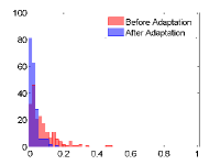
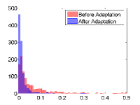
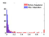
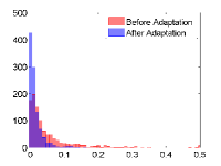
In this experiment, we analyze the statistics of the output of one shallow layer (the output of second convolution layer) and one deep layer (the output of last Inception module before ReLU) in the network. In particular, we compute the distance of source domain distribution and target domain distribution before and after adaptation. We denote each feature as , and assume that the output of each feature generally follows a Gaussian distribution with mean and variance . Then we use the symmetric KL divergence as our metric:
| (3) | ||||
We plot the distribution of the distances in Fig. 3. Our method reduces the domain discrepancy in both shallow layer and deep layer. We also report the quantitative results in Table. 4. This experiment once again verifies the effectiveness of the proposed method.
| A W | A W | A D | A D | |
|---|---|---|---|---|
| shallow | deep | shallow | deep | |
| Before Adapt | 0.0716 | 0.0614 | 0.2307 | 0.0502 |
| After Adapt | 0.0227 | 0.0134 | 0.0266 | 0.0140 |
4.3.2 Sensitivity to Target Domain Size.
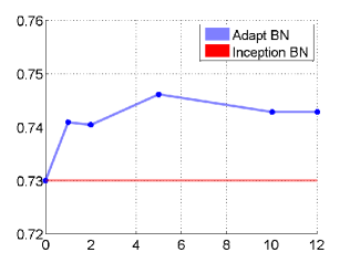
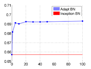
Since the key of our method is to calculate the mean and variance of the target domain on different BN layers, it is very natural to ask how many target images is necessary to obtain stable statistics. In this experiment, we randomly select a subset of images in target domain to calculate the statistics and then evaluate the performance on the whole target set. Fig. 4 illustrates the effect of using different number of batches. The results demonstrate that our method can obtain good results when using only a small part of the target examples. It should also be noted that in the extremal case of one batch of target images, our method still achieves better results than the baseline. This is valuable in practical use since a large number of target images are often not available.
4.4 Practical Application for Cloud Detection in Remote Sensing Images
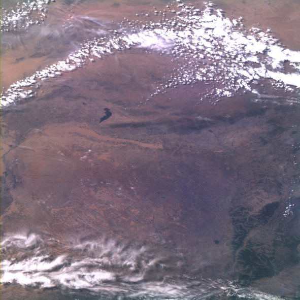
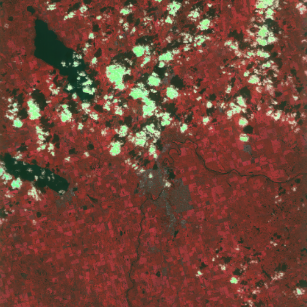
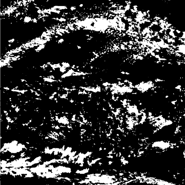
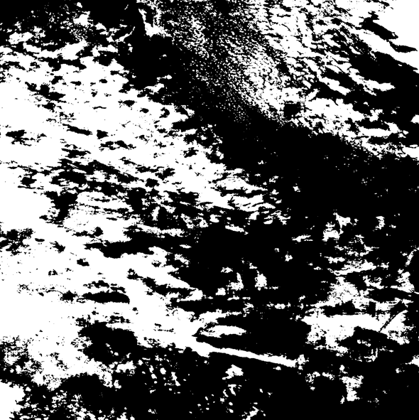
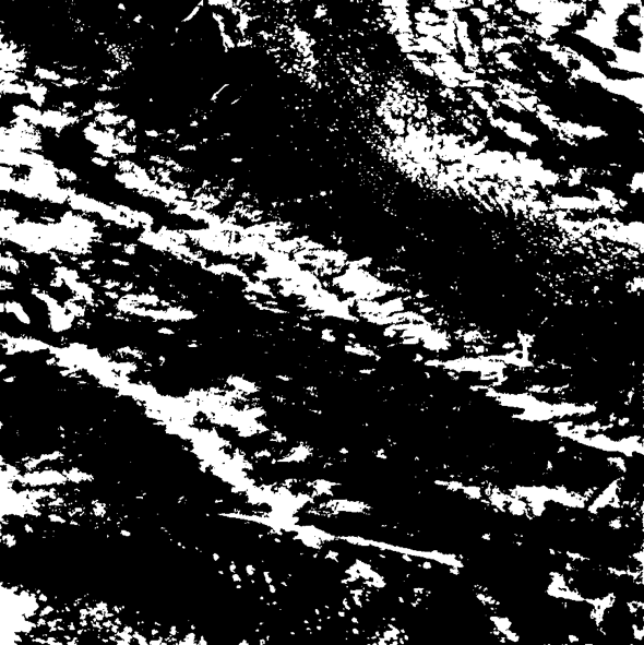
In this section, we further demonstrate the effectiveness of AdaBN on a practical problem: Cloud Detection in Remote Sensing Images. Since remote sensing images are taken by different satellites with different sensors and resolutions, the captured images are visually different in texture, color, and value range distributions, as shown in Fig. 5. How to adapt a model trained on one satellite to another satellite images is naturally a domain adaptation problem.
Our task here is to identify cloud from the remote sensing images, which can be regarded as a semantic segmentation task. The experiment is taken under a self-collected dataset, which includes three image sets, from GF2, GF1 and Tianhui satellites. Each image set contains 635, 324 and 113 images with resolution over 6000x6000 pixels respectively. We name the three different datasets following the satellite names. GF2 dataset is used as the training dataset while GF1 and Tianhui datasets are for testing. We use a state-of-art semantic segmentation method (Chen et al., 2016a) as our baseline model.
| Method | GF1 | Tianhui |
|---|---|---|
| Baseline | 38.95% | 14.54% |
| AdaBN | 64.50% | 29.66% |
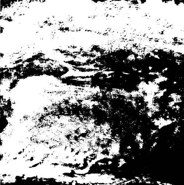
The results on GF1 and Tianhui datasets are shown in Table 5. The relatively low results of the baseline method indicate that there exists large distribution disparity among images from different satellites. Thus, the significant improvement after applying AdaBN reveals the effectiveness of our method. Some of the visual results are shown in Fig. 6. Since other domain adaptation methods require either additional optimization steps and extra components ( MMD) or post-processing distribution alignment (like CORAL), it is very hard to apply these methods from image classification to this large-size (6000x6000) segmentation problem. Comparatively, besides the effective performance, our method needs no extra parameters and very few computations over the whole adaptation process.



5 Conclusion and Future Works
In this paper, we have introduced a simple yet effective approach for domain adaptation on batch normalized neural networks. Besides its original uses, we have exploited another functionality of Batch Normalization (BN) layer: domain adaptation. The main idea is to replace the statistics of each BN layer in source domain with those in target domain. The proposed method is easy to implement and parameter-free, and it takes almost no effort to extend to multiple source domains and semi-supervised settings. Our method established new state-of-the-art results on both single and multiple source(s) domain adaptation settings on standard benchmarks. At last, the experiments on cloud detection for large-size remote sensing images further demonstrate the effectiveness of our method in practical use. We believe our method opens up a new direction for domain adaptation.
In contrary to other methods that use Maximum Mean Discrepancy (MMD) or domain confusion loss to update the weights in CNN for domain adaptation, our method only modifies the statistics of BN layer. Therefore, our method is fully complementary to other existing deep learning based methods. It is interesting to see how these different methods can be unified under one framework.
References
- Aljundi et al. (2015) Rahaf Aljundi, Rémi Emonet, Damien Muselet, and Marc Sebban. Landmarks-based kernelized subspace alignment for unsupervised domain adaptation. In CVPR, 2015.
- Baktashmotlagh et al. (2013) Mahsa Baktashmotlagh, Mehrtash Harandi, Brian Lovell, and Mathieu Salzmann. Unsupervised domain adaptation by domain invariant projection. In ICCV, pp. 769–776, 2013.
- Beijbom (2012) Oscar Beijbom. Domain adaptations for computer vision applications. arXiv preprint arXiv:1211.4860, 2012.
- Bergamo & Torresani (2010) Alessandro Bergamo and Lorenzo Torresani. Exploiting weakly-labeled web images to improve object classification: a domain adaptation approach. In NIPS, pp. 181–189, 2010.
- Bousmalis et al. (2016) Konstantinos Bousmalis, George Trigeorgis, Nathan Silberman, Dilip Krishnan, and Dumitru Erhan. Domain separation networks. NIPS, 2016.
- Chen et al. (2016a) Liang-Chieh Chen, George Papandreou, Iasonas Kokkinos, Kevin Murphy, and Alan L Yuille. Deeplab: Semantic image segmentation with deep convolutional nets, atrous convolution, and fully connected crfs. arXiv preprint arXiv:1606.00915, 2016a.
- Chen et al. (2016b) Tianqi Chen, Mu Li, Yutian Li, Min Lin, Naiyan Wang, Minjie Wang, Tianjun Xiao, Bing Xu, Chiyuan Zhang, and Zheng Zhang. MXNet: A flexible and efficient machine learning library for heterogeneous distributed systems. NIPS Workshop on Machine Learning Systems, 2016b.
- Chopra et al. (2013) Sumit Chopra, Suhrid Balakrishnan, and Raghuraman Gopalan. DLID: Deep learning for domain adaptation by interpolating between domains. In ICML Workshop on Challenges in Representation Learning, volume 2, 2013.
- Donahue et al. (2014) Jeff Donahue, Yangqing Jia, Oriol Vinyals, Judy Hoffman, Ning Zhang, Eric Tzeng, and Trevor Darrell. DeCAF: A deep convolutional activation feature for generic visual recognition. In ICML, pp. 647–655, 2014.
- Donald (1999) E Knuth Donald. The art of computer programming. Sorting and searching, 3:426–458, 1999.
- Fernando et al. (2013) Basura Fernando, Amaury Habrard, Marc Sebban, and Tinne Tuytelaars. Unsupervised visual domain adaptation using subspace alignment. In ICCV, pp. 2960–2967, 2013.
- Ganin & Lempitsky (2015) Yaroslav Ganin and Victor Lempitsky. Unsupervised domain adaptation by backpropagation. In ICML, pp. 1180–1189, 2015.
- Ghifary et al. (2014) Muhammad Ghifary, W Bastiaan Kleijn, and Mengjie Zhang. Domain adaptive neural networks for object recognition. In PRICAI: Trends in Artificial Intelligence, pp. 898–904. 2014.
- Gong et al. (2012) Boqing Gong, Yuan Shi, Fei Sha, and Kristen Grauman. Geodesic flow kernel for unsupervised domain adaptation. In CVPR, pp. 2066–2073, 2012.
- Gong et al. (2013) Boqing Gong, Kristen Grauman, and Fei Sha. Connecting the dots with landmarks: Discriminatively learning domain-invariant features for unsupervised domain adaptation. In ICML, pp. 222–230, 2013.
- Gopalan et al. (2011) Raghuraman Gopalan, Ruonan Li, and Rama Chellappa. Domain adaptation for object recognition: An unsupervised approach. In ICCV, pp. 999–1006, 2011.
- Gretton et al. (2012) Arthur Gretton, Karsten M Borgwardt, Malte J Rasch, Bernhard Schölkopf, and Alexander Smola. A kernel two-sample test. The Journal of Machine Learning Research, 13(1):723–773, 2012.
- Griffin et al. (2007) Gregory Griffin, Alex Holub, and Pietro Perona. Caltech-256 object category dataset. 2007.
- He et al. (2016) Kaiming He, Xiangyu Zhang, Shaoqing Ren, and Jian Sun. Deep residual learning for image recognition. CVPR, 2016.
- Huang et al. (2006) Jiayuan Huang, Arthur Gretton, Karsten M Borgwardt, Bernhard Schölkopf, and Alex J Smola. Correcting sample selection bias by unlabeled data. In NIPS, pp. 601–608, 2006.
- Ioffe & Szegedy (2015) Sergey Ioffe and Christian Szegedy. Batch normalization: Accelerating deep network training by reducing internal covariate shift. In ICML, pp. 448–456, 2015.
- Jia et al. (2014) Yangqing Jia, Evan Shelhamer, Jeff Donahue, Sergey Karayev, Jonathan Long, Ross Girshick, Sergio Guadarrama, and Trevor Darrell. Caffe: Convolutional architecture for fast feature embedding. In ACM MM, pp. 675–678, 2014.
- Khosla et al. (2012) Aditya Khosla, Tinghui Zhou, Tomasz Malisiewicz, Alexei A Efros, and Antonio Torralba. Undoing the damage of dataset bias. In ECCV, pp. 158–171. 2012.
- Krizhevsky et al. (2012) Alex Krizhevsky, Ilya Sutskever, and Geoffrey E Hinton. Imagenet classification with deep convolutional neural networks. In NIPS, pp. 1097–1105, 2012.
- Long et al. (2015) Mingsheng Long, Yue Cao, Jianmin Wang, and Michael Jordan. Learning transferable features with deep adaptation networks. In ICML, pp. 97–105, 2015.
- Long et al. (2016) Mingsheng Long, Jianmin Wang, and Michael I Jordan. Unsupervised domain adaptation with residual transfer networks. In NIPS, 2016.
- Pan et al. (2011) Sinno Jialin Pan, Ivor W Tsang, James T Kwok, and Qiang Yang. Domain adaptation via transfer component analysis. IEEE Transactions on Neural Networks, 22(2):199–210, 2011.
- Patel et al. (2015) Vishal M Patel, Raghuraman Gopalan, Ruonan Li, and Rama Chellappa. Visual domain adaptation: A survey of recent advances. IEEE Signal Processing Magazine, 32(3):53–69, 2015.
- Russakovsky et al. (2015) Olga Russakovsky, Jia Deng, Hao Su, Jonathan Krause, Sanjeev Satheesh, Sean Ma, Zhiheng Huang, Andrej Karpathy, Aditya Khosla, Michael Bernstein, et al. ImageNet large scale visual recognition challenge. International Journal of Computer Vision, 115(3):211–252, 2015.
- Saenko et al. (2010) Kate Saenko, Brian Kulis, Mario Fritz, and Trevor Darrell. Adapting visual category models to new domains. In ECCV, pp. 213–226. 2010.
- Shimodaira (2000) Hidetoshi Shimodaira. Improving predictive inference under covariate shift by weighting the log-likelihood function. Journal of statistical planning and inference, 90(2):227–244, 2000.
- Sun & Saenko (2016) Baochen Sun and Kate Saenko. Deep coral: Correlation alignment for deep domain adaptation. arXiv preprint arXiv:1607.01719, 2016.
- Sun et al. (2016) Baochen Sun, Jiashi Feng, and Kate Saenko. Return of frustratingly easy domain adaptation. AAAI, 2016.
- Szegedy et al. (2015) Christian Szegedy, Vincent Vanhoucke, Sergey Ioffe, Jonathon Shlens, and Zbigniew Wojna. Rethinking the inception architecture for computer vision. arXiv preprint arXiv:1512.00567, 2015.
- Tommasi et al. (2015) Tatiana Tommasi, Novi Patricia, Barbara Caputo, and Tinne Tuytelaars. A deeper look at dataset bias. German Conference on Pattern Recognition, 2015.
- Torralba & Efros (2011) Antonio Torralba and Alexei A Efros. Unbiased look at dataset bias. In CVPR, pp. 1521–1528, 2011.
- Tzeng et al. (2014) Eric Tzeng, Judy Hoffman, Ning Zhang, Kate Saenko, and Trevor Darrell. Deep domain confusion: Maximizing for domain invariance. arXiv preprint arXiv:1412.3474, 2014.
- Tzeng et al. (2015) Eric Tzeng, Judy Hoffman, Trevor Darrell, and Kate Saenko. Simultaneous deep transfer across domains and tasks. In ICCV, pp. 4068–4076, 2015.
- Van der Maaten & Hinton (2008) Laurens Van der Maaten and Geoffrey Hinton. Visualizing data using t-sne. Journal of Machine Learning Research, 9(2579-2605):85, 2008.
- Yosinski et al. (2014) Jason Yosinski, Jeff Clune, Yoshua Bengio, and Hod Lipson. How transferable are features in deep neural networks? In NIPS, pp. 3320–3328, 2014.