\ieeecopyright

????–????/??$??.?? © ???? IEEE \lognumberxxxxxxx \pubitemidentS ????–????(??)?????–? \loginfoManuscript received ??? ??, ????.

\confplacedate

????, ???, ??? ??–??, ????

A Novel Method for the Extrinsic Calibration of
a 2D Laser Rangefinder and a Camera

Wenbo Dong\memberStudent Member A preliminary version of this work was presented in [27]. This extended version includes spatial-ambiguity explanation, the complete proof of uniqueness, the analytical solution, as well as calibration details and additional experiments.This work is supported in part by NSF Award 1317788, USDA Award MIN-98-G02 and the MnDrive initiative.    and Volkan Isler\memberSenior Member\authorinfoW. Dong and V. Isler are with the Department of Computer Science and Engineering, University of Minnesota, Twin Cities, MN, 55455, USA. E-mail: {dong, isler}@cs.umn.edu
Abstract

We present a novel method for extrinsically calibrating a camera and a 2D Laser Rangefinder (LRF) whose beams are invisible from the camera image. We show that point-to-plane constraints from a single observation of a V-shaped calibration pattern composed of two non-coplanar triangles suffice to uniquely constrain the relative pose between two sensors. Next, we present an approach to obtain analytical solutions using point-to-plane constraints from single or multiple observations. Along the way, we also show that previous solutions, in contrast to our method, have inherent ambiguities and therefore must rely on a good initial estimate. Real and synthetic experiments validate our method and show that it achieves better accuracy than previous methods.

keywords:
2D Laser Rangefinder (LRF), Camera, Extrinsic Calibration, Analytical Solution.
journal:

1 Introduction

\PARstart

Many robotics systems rely on cameras and laser range finders to compute environment geometry [1]. Two dimensional (2D) Laser Range Finders (LRFs) which measure depth along a single plane are commonly used due to their low weight, low cost and low power requirements.

Taking advantage of measurements from an LRF or a LIDAR combined with a camera, however, requires precise knowledge of the relative pose (orientation and position) between them. This is a classical extrinsic calibration problem where the objective is to determine the transformation between two coordinate frames. Establishing correspondences between two sensors is easier for 3D LIDARs since distinct features can be identified both among laser points and in the camera image. Existing methods include 3D LIDAR-camera calibration by using a circle-based calibration target [2] and an arbitrary trihedron [3].

Extrinsic calibration of a 2D LRF is more challenging because a 2D LRF produces only a single scanning plane for each pose which is invisible from the regular camera. This makes it difficult to find correspondences. Therefore, additional constraints must be used. We note that if we were given the correspondences between laser points and their images (e.g. IR camera) the extrinsic calibration problem reduces to a standard Pn𝑛nP (Perspective-n-Point) computation [4]. However, in our case, these correspondences are unknown.

There is a large body of work on the LRF-camera calibration. One of the earliest methods is presented by Zhang and Pless [5] using points-on-plane constraints. However, only two degrees of freedom are constrained for the relative pose between the camera and the LRF from a single input observation. Therefore, this method requires a large number of different observations with a wide range of views (more than 20 snapshots) for accuracy. Vasconcelos et al. [6] presented a minimal solution by forming a perspective-three-point (P3P) problem to address disadvantages in [5]. Zhou [7] further proposed an algebraic method for extrinsic calibration. Both techniques require multiple observations (at least three), and have inherent degeneracy where intersecting lines of two planes with the third plane are parallel, and three intersecting points of laser segments from three input observations are on a danger cylinder.
Refer to caption
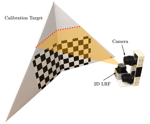
Figure 1: The calibration system incorporating a calibration target and a capture rig; Left: The calibration target formed by two triangular boards with a checkerboard on each triangle; Right: The capture rig consisting of a 2D LRF and stereo cameras. (Only one camera is involved in the calibration problem, the other is just for testing in real experiment.)
Refer to caption
Figure 2: A single pair of LRF-camera observations of our calibration target with the definition of parameters for geometry constraints. (a): The output of the 2D LRF-camera calibration is the relative transformation 𝐑LCsubscriptsuperscript𝐑𝐶𝐿{{}_{L}^{C}}\mathbf{R} and 𝐭CL{{}^{C}}\mathbf{t}{{}_{L}}. (b): The input data from the LRF are three laser points 𝐩1Lsuperscriptsubscript𝐩1𝐿{{}^{L}}\mathbf{p}_{1}, 𝐩2Lsuperscriptsubscript𝐩2𝐿{{}^{L}}\mathbf{p}_{2} and 𝐩3Lsuperscriptsubscript𝐩3𝐿{{}^{L}}\mathbf{p}_{3}. (c): Two input normals from the camera are 𝐧1Csuperscriptsubscript𝐧1𝐶{{}^{C}}\mathbf{n}_{1} and 𝐧2Csuperscriptsubscript𝐧2𝐶{{}^{C}}\mathbf{n}_{2}. (d): The other input data from the camera are two normals 𝐧3Csuperscriptsubscript𝐧3𝐶{{}^{C}}\mathbf{n}_{3} and 𝐧4Csuperscriptsubscript𝐧4𝐶{{}^{C}}\mathbf{n}_{4} and two distances d1subscript𝑑1d_{1} and d2subscript𝑑2d_{2}.

With point-on-line constraints, the approaches in [8] and  [9] use a black triangular board and a V-shaped calibration target respectively. The results from these two methods are not accurate due to the sparse sampling of laser points. Further, a large number (usually more than 100) of images are needed to compensate for the lack of constraints for each input observation. Based on the ideas in [8] and [9] (minimizing the projection distance on the image between intersected laser points and the feature lines), the authors in [10] also propose to use a V-shaped calibration target. They increase the laser points’ sampling for each observation by introducing more feature lines and virtual end-points, but the same drawback still exists as in [9] and [10]. Therefore, they still need a large amount (around 50) of different observations to achieve a reasonable result.

The method in [11] provides an analytical solution using a white board with a black band in the middle. It needs only six different observations. Similarly, the authors in [12] give an analytical solution to this problem using a white board with a black line in the middle. Compared with [11], it further computes the optimal least-squares solution to improve the robustness to noise. The analytical solutions in [11] and [12] are obtained by minimizing the sum of points-on-plane errors, where only perspective planes from the image are considered instead of general 3D planes. However, both of these two methods still cannot avoid using a large number of different observations for accuracy because of the insufficient constraints for each input observation.

The work described in [13], presents an approach which only requires the observation of a scene corner (orthogonal trihedron) commonly found in human-made environments. This method builds line-to-plane and point-to-plane constraints, which requires at least two input observations. However, the calibration accuracy highly depends right angles between three orthogonal planes, which are difficult to be made exactly 90superscript9090^{\circ} in practice. When multiple observations from different views are needed for additional accuracy, the right angle between two walls often affects the laser measurement: scanned laser line on one wall is curved if laser beams point almost perpendicular towards the other wall for a good view. Our method accommodates an arbitrary obtuse angle in our calibration target (See Fig. 1) so that it can adjust the view angle between the pattern and linear beams.

The authors in [14] further extend the work [13] by deriving a minimal solution from a single input observation. The solution, however, is obtained by two procedures (calibration between the trihedron and the LRF, and calibration between the trihedron and the camera), and thus has accumulated error due to the data noise in each procedure. Specifically, in calibration between the trihedron and the camera, they determine the scale of the translation by using the actual length of two edges of the trihedron which is inconvenient to be built and difficult to be measured accurately.

In theory, LRF-camera calibration from a single input observation is important since it means that the geometric constraints from a single view is sufficient. In practice, it further implies that users, when taking multiple input observations for further accuracy, do not need to be concerned about degenerate cases in which the input observation is invalid. Our triangular V-shaped calibration target (See Fig. 1) has two checkerboards, which are simultaneously and accurately estimated in camera calibration. Further, the angle between two triangular boards of the target can be arbitrary which makes it convenient to build. We study this extrinsic calibration problem and make the following contributions:

  • We show that by minimizing the sum of points-on-plane errors, a single observation of two non-coplanar triangles sharing a common side (See Fig. 1) suffices to unambiguously solve the calibration problem.

  • Even though planar, triangular or V-shaped rectangular patterns have already been proposed to solve the calibration problem, we show that previous methods do not sufficiently constrain the calibration problem to allow for a unique solution. Therefore, they rely on a large number of measurements and a good initial estimate.

  • We also present a robust analytical solution to the system of points-on-plane constraints for calibration from a single observation in the presence of noise.

  • For additional accuracy, we show that by using only a few additional observations, our method achieves significantly smaller error than existing methods.

2 Spatial Ambiguities In Previous Methods

The objective of 2D LRF-camera calibration is to obtain the relative pose between these two sensors: the orientation 𝐑LCsubscriptsuperscript𝐑𝐶𝐿{{}_{L}^{C}}\mathbf{R} and position 𝐭CL{{}^{C}}\mathbf{t}{{}_{L}} of the LRF frame {L}𝐿\{L\} with respect to (w.r.t.) the camera frame {C}𝐶\{C\} (See Fig. 2). Spatial ambiguity means that there are infinite solutions for 𝐑LCsubscriptsuperscript𝐑𝐶𝐿{{}_{L}^{C}}\mathbf{R} and 𝐭CL{{}^{C}}\mathbf{t}{{}_{L}} from a single input observation of the calibration target.

Without loss of generality, the laser scanning plane is defined as the plane YL=0subscript𝑌𝐿0Y_{L}=0 such that we do not have an explicit dependence on the second column vector 𝐫2subscript𝐫2\mathbf{r}_{2} of 𝐑LCsubscriptsuperscript𝐑𝐶𝐿{{}_{L}^{C}}\mathbf{R} when a 3D laser point 𝐩L=[xL,0,zL]superscript𝐩𝐿superscriptsubscript𝑥𝐿0subscript𝑧𝐿top{{}^{L}}\mathbf{p}=[x_{L},0,z_{L}]^{\top} is transformed to the point 𝐩C=[xC,yC,zC]superscript𝐩𝐶superscriptsubscript𝑥𝐶subscript𝑦𝐶subscript𝑧𝐶top{{}^{C}}\mathbf{p}=[x_{C},y_{C},z_{C}]^{\top} in the camera frame by 𝐩C=𝐑LC𝐩L+𝐭LCsuperscript𝐩𝐶subscriptsuperscript𝐑𝐶𝐿superscript𝐩𝐿superscriptsubscript𝐭𝐿𝐶{{}^{C}}\mathbf{p}={{}_{L}^{C}}\mathbf{R}\cdot{{}^{L}}\mathbf{p}+{{}^{C}}\mathbf{t}_{L}. Since 𝐑LCsubscriptsuperscript𝐑𝐶𝐿{{}_{L}^{C}}\mathbf{R} is an orthonormal matrix, we have three constraints for its first and third columns (𝐫1subscript𝐫1\mathbf{r}_{1} and 𝐫3subscript𝐫3\mathbf{r}_{3})

𝐫3𝐫3=1,𝐫1𝐫1=1,𝐫3𝐫1=0.formulae-sequencesuperscriptsubscript𝐫3topsubscript𝐫31formulae-sequencesuperscriptsubscript𝐫1topsubscript𝐫11superscriptsubscript𝐫3topsubscript𝐫10\mathbf{r}_{3}^{\top}\mathbf{r}_{3}=1,\quad\mathbf{r}_{1}^{\top}\mathbf{r}_{1}=1,\quad\mathbf{r}_{3}^{\top}\mathbf{r}_{1}=0. (1)

Thus, we need at least six additional geometry constraints for solving nine unknowns (in 𝐫1subscript𝐫1\mathbf{r}_{1}, 𝐫3subscript𝐫3\mathbf{r}_{3} and 𝐭CL{{}^{C}}\mathbf{t}{{}_{L}}).

Refer to caption
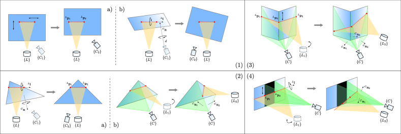
Figure 3: Existing methods do not sufficiently constrain the problem from a single input observation. (1): In the approach of Zhang and Pless [5], essentially, only two laser points 𝐩1Lsuperscriptsubscript𝐩1𝐿{{}^{L}}\mathbf{p}_{1} and 𝐩2Lsuperscriptsubscript𝐩2𝐿{{}^{L}}\mathbf{p}_{2} are constrained on the calibration board, where d𝑑d is the distance from the camera to the board. a): The camera frame C1subscript𝐶1C_{1} with the board can be moved horizontally and vertically along the board to C2subscript𝐶2C_{2}. b): The camera frame C1subscript𝐶1C_{1} with the board are first rotated along the board normal 𝐧Csuperscript𝐧𝐶{{}^{C}}\mathbf{n} and then rotated along the laser line direction 𝐥Lsuperscript𝐥𝐿{{}^{L}}\mathbf{l} to reach C2subscript𝐶2C_{2}. (2): In the approach of Li et al. [8], only two geometry constraints are obtained. a): The camera frame C1subscript𝐶1C_{1} with the triangular calibration board are first rotated long the board normal 𝐧Csuperscript𝐧𝐶{{}^{C}}\mathbf{n} and then rotated along the laser line direction 𝐥Lsuperscript𝐥𝐿{{}^{L}}\mathbf{l} to reach C2subscript𝐶2C_{2} such that 𝐩1Lsuperscriptsubscript𝐩1𝐿{{}^{L}}\mathbf{p}_{1} and 𝐩2Lsuperscriptsubscript𝐩2𝐿{{}^{L}}\mathbf{p}_{2} are still on the border lines. b): The LRF frame L1subscript𝐿1L_{1} can be moved and rotated to get L2subscript𝐿2L_{2} as long as 𝐩1Lsuperscriptsubscript𝐩1𝐿{{}^{L}}\mathbf{p}_{1} and 𝐩2Lsuperscriptsubscript𝐩2𝐿{{}^{L}}\mathbf{p}_{2} are on green 3D perspective planes of 2D detected board edges. (3): In methods [9] and [10], three geometry constraints are 𝐧iC(𝐑LC𝐩iL+𝐭C)L=0{{}^{C}}\mathbf{n}_{i}^{\top}\left({{}_{L}^{C}}\mathbf{R}\cdot{{}^{L}}\mathbf{p}_{i}+{{}^{C}}\mathbf{t}{{}_{L}}\right)=0 where 𝐧iCsuperscriptsubscript𝐧𝑖𝐶{{}^{C}}\mathbf{n}_{i} with i=1,2,3𝑖123i=1,2,3 are three normals of 3D perspective planes. To reach L2subscript𝐿2L_{2}, the LRF frame L1subscript𝐿1L_{1} with the laser line segments can be moved vertically along the calibration target and then rotated as long as 𝐩1Lsuperscriptsubscript𝐩1𝐿{{}^{L}}\mathbf{p}_{1}, 𝐩2Lsuperscriptsubscript𝐩2𝐿{{}^{L}}\mathbf{p}_{2} and 𝐩3Lsuperscriptsubscript𝐩3𝐿{{}^{L}}\mathbf{p}_{3} lie on their green 3D perspective planes. (4): In approaches [12] and [11], geometry constraints (up to two) are 𝐧iC(𝐑LC𝐩iL+𝐭C)L=0{{}^{C}}\mathbf{n}_{i}^{\top}\left({{}_{L}^{C}}\mathbf{R}\cdot{{}^{L}}\mathbf{p}_{i}+{{}^{C}}\mathbf{t}{{}_{L}}\right)=0 where 𝐧iCsuperscriptsubscript𝐧𝑖𝐶{{}^{C}}\mathbf{n}_{i} with i=1,2𝑖12i=1,2 are two normals of 3D perspective planes. Base on the same principle, the LRF frame L1subscript𝐿1L_{1}, in order to get L2subscript𝐿2L_{2}, can be moved vertically along the board, rotated along the laser line direction 𝐥Lsuperscript𝐥𝐿{{}^{L}}\mathbf{l}, and also rotated together with the line segment to make sure 𝐩1Lsuperscriptsubscript𝐩1𝐿{{}^{L}}\mathbf{p}_{1} and 𝐩2Lsuperscriptsubscript𝐩2𝐿{{}^{L}}\mathbf{p}_{2} still lie on corresponding perspective planes.

The spatial ambiguity is caused by the lack of sufficient geometric constraints from a single input observation. The disadvantage of insufficient constraints is that a large number of snapshots of the calibration target from different views are needed to reduce the ambiguity by minimizing the geometry cost function. A good initial estimate thus must be required otherwise the solution may converge to a local minimum which may not be the global minimum. However, this good initial estimate is not guaranteed in existing methods. Based on different type of calibration targets, previous methods can be classified into four categories: planar board with a checkerboard, triangle board, V-sharped target and rectangular board with a line or a band. Next, we detail the spatial ambiguity in each category.

Planar Board with a Checkerboard: In the approach of Zhang and Pless [5], all laser points must lie on the planar calibration pattern, described as 𝐧C(𝐑LC𝐩iL+𝐭C)L=d{{}^{C}}\mathbf{n}^{\top}\left({{}_{L}^{C}}\mathbf{R}\cdot{{}^{L}}\mathbf{p}_{i}+{{}^{C}}\mathbf{t}{{}_{L}}\right)=d in Fig. 3. Essentially, only two laser points are constrained from the single snapshot (two geometry constraints), and constraints of the rest of the laser points are redundant since they all belong to the same line segment. For the relative pose of the 2D LRF-camera pair, only two out of six degrees of freedom are constrained. The remaining four degrees have ambiguity such that there are infinite solutions for 𝐑LCsubscriptsuperscript𝐑𝐶𝐿{{}_{L}^{C}}\mathbf{R} and 𝐭CL{{}^{C}}\mathbf{t}{{}_{L}}. As shown in Fig. 3, the calibration board together with the camera frame can be moved horizontally and vertically, and also can be rotated along two different axes without violating the geometry constraints.

Triangle Board: The work of Li et al. [8] by using a triangular board does not improve the constraints in the method by Zhang and Pless [5]: two laser end points 𝐩1Lsuperscriptsubscript𝐩1𝐿{{}^{L}}\mathbf{p}_{1} and 𝐩2Lsuperscriptsubscript𝐩2𝐿{{}^{L}}\mathbf{p}_{2} must lie on their corresponding border lines detected from the camera, represented as 𝐧iC(𝐑LC𝐩iL+𝐭C)L=0{{}^{C}}\mathbf{n}_{i}^{\top}\left({{}_{L}^{C}}\mathbf{R}\cdot{{}^{L}}\mathbf{p}_{i}+{{}^{C}}\mathbf{t}{{}_{L}}\right)=0 where 𝐧iCsuperscriptsubscript𝐧𝑖𝐶{{}^{C}}\mathbf{n}_{i} with i=1,2𝑖12i=1,2 are the normals of the 3D perspective planes of 2D detected border lines. These two constraints remove the ambiguity of the horizontal translation and “triangular plane” removes the ambiguity of the vertical translation for 𝐭CL{{}^{C}}\mathbf{t}{{}_{L}}. However, there are still three degrees of freedom that remain ambiguous for 𝐑LCsubscriptsuperscript𝐑𝐶𝐿{{}_{L}^{C}}\mathbf{R} (See Fig. 3). Essentially, the drawback is that the constraints are imposed on the 2D image: there exist uncertainties for a total of four unknown elements from views of depth and orientation (two linear geometry constraints plus three nonlinear constraints for 𝐑LCsubscriptsuperscript𝐑𝐶𝐿{{}_{L}^{C}}\mathbf{R} to solve nine unknowns). Additional details are explained in Section 4.

V-sharped Target: The calibration target in [9] and [10] is formed as V-shaped by two rectangular boards. Three laser end points 𝐩1Lsuperscriptsubscript𝐩1𝐿{{}^{L}}\mathbf{p}_{1}, 𝐩2Lsuperscriptsubscript𝐩2𝐿{{}^{L}}\mathbf{p}_{2} and 𝐩3Lsuperscriptsubscript𝐩3𝐿{{}^{L}}\mathbf{p}_{3} must lie on their corresponding board edges detected from the camera. Although the geometry constraints increase to three, the same drawbacks of spatial ambiguities still exist (the vertical translation of the calibration target as in [5], and the movement of laser points along their perspective planes as in [8]). See Fig. 3 for more details.

Rectangular Board with a Line or a Band: Methods in [11] and [12] can be generalized as using a rectangular board with a black band (or a line) in the middle. Two laser end points 𝐩1Lsuperscriptsubscript𝐩1𝐿{{}^{L}}\mathbf{p}_{1} and 𝐩2Lsuperscriptsubscript𝐩2𝐿{{}^{L}}\mathbf{p}_{2} must lie on their band edges detected from the camera. With no more than two geometric constraints, they also suffer from spatial ambiguities. Thus, 𝐑LCsubscriptsuperscript𝐑𝐶𝐿{{}_{L}^{C}}\mathbf{R} and 𝐭CL{{}^{C}}\mathbf{t}{{}_{L}} have infinite solutions (See Fig. 3).

In contrast to previous methods, our method builds sufficient constraints, which guarantee the uniqueness of the solution for each input observation. In theory, we can use only one snapshot to calibrate the 2D LRF-camera rig. In practice, an accurate result can be achieved with only a few snapshots (previous methods require 20 or more).

3 Geometry Constraints Formulation

Our calibration setup is shown in Fig. 2. A V-shaped calibration target is formed by two triangular boards with a checkerboard on each triangle. The angle between the two boards can be arbitrary as long as the two boards are not coplanar (the angle is 0 or 180 degree). In practice, the angle is set to arbitrarily obtuse to get good camera views of both two boards, and does not need to be known. P𝑃P, Q𝑄Q, R𝑅R and O𝑂O are four corners of the target. We define the triangles as T1=PQCsubscript𝑇1𝑃𝑄𝐶T_{1}=\bigtriangleup PQC and T2=PRCsubscript𝑇2𝑃𝑅𝐶T_{2}=\bigtriangleup PRC, and let T3=PQOsubscript𝑇3𝑃𝑄𝑂T_{3}=\bigtriangleup PQO and T4=PROsubscript𝑇4𝑃𝑅𝑂T_{4}=\bigtriangleup PRO. For each observation, the scanning plane of the LRF intersects with the three sides PQ¯¯𝑃𝑄\overline{PQ}, PR¯¯𝑃𝑅\overline{PR} and PO¯¯𝑃𝑂\overline{PO} at points 𝐩1Lsuperscriptsubscript𝐩1𝐿{{}^{L}}\mathbf{p}_{1}, 𝐩2Lsuperscriptsubscript𝐩2𝐿{{}^{L}}\mathbf{p}_{2} and 𝐩3Lsuperscriptsubscript𝐩3𝐿{{}^{L}}\mathbf{p}_{3} respectively in the LRF frame. Moreover, the camera and LRF should be either synchronized or held stationary during data collection. The camera is modeled by the standard pinhole model. We ignore lens distortions in the rest of the paper, and assume that the images have already been undistorted, e.g. using the functions from MATLAB Camera Calibration Toolbox [15].

Each observation of the calibration target consists of an image acquired from the camera and a single scan obtained from the LRF. The output of our calibration method is the relative transformation (𝐑LCsubscriptsuperscript𝐑𝐶𝐿{{}_{L}^{C}}\mathbf{R} and position 𝐭CL{{}^{C}}\mathbf{t}{{}_{L}}) between the 2D LRF and the camera. As shown in Fig. 2, the input features from a single observation are: 1) three laser points 𝐩1Lsuperscriptsubscript𝐩1𝐿{{}^{L}}\mathbf{p}_{1}, 𝐩2Lsuperscriptsubscript𝐩2𝐿{{}^{L}}\mathbf{p}_{2} and 𝐩3Lsuperscriptsubscript𝐩3𝐿{{}^{L}}\mathbf{p}_{3} from the LRF; 2) two unit normals 𝐧1Csuperscriptsubscript𝐧1𝐶{{}^{C}}\mathbf{n}_{1} and 𝐧2Csuperscriptsubscript𝐧2𝐶{{}^{C}}\mathbf{n}_{2} of perspective planes T1subscript𝑇1T_{1}, T2subscript𝑇2T_{2} from the camera; 3) two unit normals 𝐧3Csuperscriptsubscript𝐧3𝐶{{}^{C}}\mathbf{n}_{3} and 𝐧4Csuperscriptsubscript𝐧4𝐶{{}^{C}}\mathbf{n}_{4} of board planes T3subscript𝑇3T_{3} and T4subscript𝑇4T_{4} in the camera frame, and two distances d1subscript𝑑1d_{1} and d2subscript𝑑2d_{2} from the camera to planes T3subscript𝑇3T_{3} and T4subscript𝑇4T_{4} respectively. Further details of feature extraction are described in Section 6.

A single laser scan consists of a depth value for each angle at which the depth was sensed. In the LRF frame, we assume that the sensor is at its origin L𝐿L. Let us express the feature points 𝐩iLsuperscriptsubscript𝐩𝑖𝐿{{}^{L}}\mathbf{p}_{i} as [xi,0,zi]superscriptsubscript𝑥𝑖0subscript𝑧𝑖top[x_{i},0,z_{i}]^{\top}, where i={1,2,3}𝑖123i=\{1,2,3\} are the indices of the feature points. Let the feature normals 𝐧jsubscript𝐧𝑗\mathbf{n}_{j} of planes Tjsubscript𝑇𝑗T_{j} be [aj,bj,cj]superscriptsubscript𝑎𝑗subscript𝑏𝑗subscript𝑐𝑗top[a_{j},b_{j},c_{j}]^{\top}, where j={1,2,3,4}𝑗1234j=\{1,2,3,4\}. We now have a correspondence between a 3D point in LRF frame and a plane in camera frame. Thus, our constraint is that the laser point, transformed to the camera frame, must lie on the corresponding plane, which can be divided into three parts.

First, laser points 𝐩1Lsuperscriptsubscript𝐩1𝐿{{}^{L}}\mathbf{p}_{1} and 𝐩2Lsuperscriptsubscript𝐩2𝐿{{}^{L}}\mathbf{p}_{2} must lie on the planes T1subscript𝑇1T_{1} and T2subscript𝑇2T_{2}, respectively. Then, the first two constraints have the form

𝐧iC(𝐑LC𝐩iL+𝐭C)L=0,i={1,2}{{}^{C}}\mathbf{n}_{i}^{\top}\left({{}_{L}^{C}}\mathbf{R}\cdot{{}^{L}}\mathbf{p}_{i}+{{}^{C}}\mathbf{t}{{}_{L}}\right)=0,\quad i=\{1,2\} (2)

where 𝐑LCSO(3)subscriptsuperscript𝐑𝐶𝐿𝑆𝑂3{{}_{L}^{C}}\mathbf{R}\in SO(3) and 𝐭CL{{}^{C}}\mathbf{t}{{}_{L}} are the unknowns. Second, for laser points 𝐩1Lsuperscriptsubscript𝐩1𝐿{{}^{L}}\mathbf{p}_{1} and 𝐩3Lsuperscriptsubscript𝐩3𝐿{{}^{L}}\mathbf{p}_{3}, they must both lie on the plane T3subscript𝑇3T_{3}. Then, we have other two constraints

𝐧3C(𝐑LC𝐩jL+𝐭C)L=d1,j={1,3}.{{}^{C}}\mathbf{n}_{3}^{\top}\left({{}_{L}^{C}}\mathbf{R}\cdot{{}^{L}}\mathbf{p}_{j}+{{}^{C}}\mathbf{t}{{}_{L}}\right)=d_{1},\quad j=\{1,3\}. (3)

Similarly, laser points 𝐩2Lsuperscriptsubscript𝐩2𝐿{{}^{L}}\mathbf{p}_{2} and 𝐩3Lsuperscriptsubscript𝐩3𝐿{{}^{L}}\mathbf{p}_{3} must both lie on the plane T4subscript𝑇4T_{4}. This gives two more constraints:

𝐧4C(𝐑LC𝐩kL+𝐭C)L=d2,k={2,3}.{{}^{C}}\mathbf{n}_{4}^{\top}\left({{}_{L}^{C}}\mathbf{R}\cdot{{}^{L}}\mathbf{p}_{k}+{{}^{C}}\mathbf{t}{{}_{L}}\right)=d_{2},\quad k=\{2,3\}. (4)

As stated in Section 2, once we solve for two columns 𝐫1subscript𝐫1\mathbf{r}_{1} and 𝐫3subscript𝐫3\mathbf{r}_{3} of 𝐑LCsubscriptsuperscript𝐑𝐶𝐿{{}_{L}^{C}}\mathbf{R}, the second column 𝐫2subscript𝐫2\mathbf{r}_{2} can be obtained by

𝐫2=𝐫3×𝐫1.subscript𝐫2subscript𝐫3subscript𝐫1\mathbf{r}_{2}=\mathbf{r}_{3}\times\mathbf{r}_{1}. (5)

To summarize, we have nine unknowns (in 𝐫1subscript𝐫1\mathbf{r}_{1}, 𝐫3subscript𝐫3\mathbf{r}_{3} and 𝐭CL{{}^{C}}\mathbf{t}{{}_{L}}) and a system of six linear (Eqs. (2)-(4)) and three nonlinear equations (Eq. (1)). In the next section, we show that these nine constraints are independent and hence sufficient to obtain a solution.

4 Uniqueness Of The Solution

In this section, we prove that the features from a single observation of our calibration target constrain the calibration problem to a finite number of solutions.

For a single observation of the calibration target, our method builds up a system of Eqs. (1)-(4). In order to prove the proposed method does not induce any ambiguity, the nine equations must be independent. We show that the first six linear equations are linearly independent. Since the other three nonlinear equations have no relationship with geometry constraints, they are independent from the first six linear equations.

From the constraints formulation, the six linear equations can be expressed as the following form

𝒜𝒳=,𝒳=[𝐭C,L𝐫1,𝐫3],\mathcal{A}\mathcal{X}=\mathcal{B},\quad\mathcal{X}=[{{}^{C}}\mathbf{t}{{}_{L}}^{\top},\mathbf{r}_{1}^{\top},\mathbf{r}_{3}^{\top}]^{\top}, (6)

where 𝒳𝒳\mathcal{X} is the vector of unknowns with 𝐭C=L[t1,t2,t3]{{}^{C}}\mathbf{t}{{}_{L}}=[t_{1},t_{2},t_{3}]^{\top}, 𝐫1=[r11,r21,r31]subscript𝐫1superscriptsubscript𝑟11subscript𝑟21subscript𝑟31top\mathbf{r}_{1}=[r_{11},r_{21},r_{31}]^{\top} and 𝐫3=[r13,r23,r33]subscript𝐫3superscriptsubscript𝑟13subscript𝑟23subscript𝑟33top\mathbf{r}_{3}=[r_{13},r_{23},r_{33}]^{\top}, \mathcal{B} is the distance vector denoted as =[0,0,d1,d1,d2,d2]superscript00subscript𝑑1subscript𝑑1subscript𝑑2subscript𝑑2top\mathcal{B}=[0,0,d_{1},d_{1},d_{2},d_{2}]^{\top}, and 𝒜𝒜\mathcal{A} is the coefficient matrix whose elements are expressed using components from 𝐧iCsuperscriptsubscript𝐧𝑖𝐶{}^{C}\mathbf{n}_{i} and 𝐩jLsuperscriptsubscript𝐩𝑗𝐿{}^{L}\mathbf{p}_{j} as defined in Section 3. Lemma 1 below states that the three unit vectors 𝐧1Csuperscriptsubscript𝐧1𝐶{}^{C}\mathbf{n}_{1}, 𝐧2Csuperscriptsubscript𝐧2𝐶{}^{C}\mathbf{n}_{2} and 𝐧3Csuperscriptsubscript𝐧3𝐶{}^{C}\mathbf{n}_{3} are linearly independent, which means they span the entire 3D space.

Lemma 1

Suppose 𝐧iCsuperscriptsubscript𝐧𝑖𝐶{{}^{C}}\mathbf{n}_{i} is the normal vector of plane Tisubscript𝑇𝑖T_{i} for i=1,2,3,4𝑖1234i={1,2,3,4} as defined in Fig. 2, these normal vectors in any cardinality three subset of {𝐧1C,𝐧2C,𝐧3C,𝐧4C}superscriptsubscript𝐧1𝐶superscriptsubscript𝐧2𝐶superscriptsubscript𝐧3𝐶superscriptsubscript𝐧4𝐶\{{{}^{C}}\mathbf{n}_{1},{{}^{C}}\mathbf{n}_{2},{{}^{C}}\mathbf{n}_{3},{{}^{C}}\mathbf{n}_{4}\} are linearly independent (totally four subsets: I. 𝐧1Csuperscriptsubscript𝐧1𝐶{{}^{C}}\mathbf{n}_{1}, 𝐧2Csuperscriptsubscript𝐧2𝐶{{}^{C}}\mathbf{n}_{2} and 𝐧3Csuperscriptsubscript𝐧3𝐶{{}^{C}}\mathbf{n}_{3}; II. 𝐧1Csuperscriptsubscript𝐧1𝐶{{}^{C}}\mathbf{n}_{1}, 𝐧2Csuperscriptsubscript𝐧2𝐶{{}^{C}}\mathbf{n}_{2} and 𝐧4Csuperscriptsubscript𝐧4𝐶{{}^{C}}\mathbf{n}_{4}; III. 𝐧1Csuperscriptsubscript𝐧1𝐶{{}^{C}}\mathbf{n}_{1}, 𝐧3Csuperscriptsubscript𝐧3𝐶{{}^{C}}\mathbf{n}_{3} and 𝐧4Csuperscriptsubscript𝐧4𝐶{{}^{C}}\mathbf{n}_{4}; IV. 𝐧2Csuperscriptsubscript𝐧2𝐶{{}^{C}}\mathbf{n}_{2}, 𝐧3Csuperscriptsubscript𝐧3𝐶{{}^{C}}\mathbf{n}_{3} and 𝐧4Csuperscriptsubscript𝐧4𝐶{{}^{C}}\mathbf{n}_{4}.).

The proof is presented in Appendix A.

As a corollary, the unit vector 𝐧4Csuperscriptsubscript𝐧4𝐶{}^{C}\mathbf{n}_{4} can be expressed as the combination of first three unit vectors 𝐧4C=uC𝐧1+vC𝐧2+wC𝐧3superscriptsubscript𝐧4𝐶superscript𝐶𝑢subscript𝐧1superscript𝐶𝑣subscript𝐧2superscript𝐶𝑤subscript𝐧3{}^{C}\mathbf{n}_{4}=u\cdot^{C}\mathbf{n}_{1}+v\cdot^{C}\mathbf{n}_{2}+w\cdot^{C}\mathbf{n}_{3}. This allows us to perform Gaussian elimination on Eq. (6) as follows:

  • Keep row1subscriptrow1\textit{{row}}_{1} and row2subscriptrow2\textit{{row}}_{2} unchanged, and let Row3row4subscriptRow3subscriptrow4\textit{{Row}}_{3}\leftarrow\textit{{row}}_{4};

  • Let Row4row3row4subscriptRow4subscriptrow3subscriptrow4\textit{{Row}}_{4}\leftarrow\textit{{row}}_{3}-\textit{{row}}_{4} and Row5row6row5subscriptRow5subscriptrow6subscriptrow5\textit{{Row}}_{5}\leftarrow\textit{{row}}_{6}-\textit{{row}}_{5};

  • Let Row6row5(urow1+vrow2+wrow3)subscriptRow6subscriptrow5𝑢subscriptrow1𝑣subscriptrow2𝑤subscriptrow3\textit{{Row}}_{6}\leftarrow\textit{{row}}_{5}-(u\cdot\textit{{row}}_{1}+v\cdot\textit{{row}}_{2}+w\cdot\textit{{row}}_{3}).

Here, 𝒜𝒜\mathcal{A} is transformed as

𝒜=[a1b1c1a1x1b1x1c1x1a1z1b1z1c1z1a2b2c2a2x2b2x2c2x2a2z2b2z2c2z2a3b3c3a3x1b3x1c3x1a3z1b3z1c3z1a3b3c3a3x3b3x3c3x3a3z3b3z3c3z3a4b4c4a4x2b4x2c4x2a4z2b4z2c4z2a4b4c4a4x3b4x3c4x3a4z3b4z3c4z3]𝒜¯=[𝒫α𝒬α𝟎3×3𝒫¯β|𝒬¯β]𝒜matrixsubscript𝑎1subscript𝑏1subscript𝑐1subscript𝑎1subscript𝑥1subscript𝑏1subscript𝑥1subscript𝑐1subscript𝑥1subscript𝑎1subscript𝑧1subscript𝑏1subscript𝑧1subscript𝑐1subscript𝑧1subscript𝑎2subscript𝑏2subscript𝑐2subscript𝑎2subscript𝑥2subscript𝑏2subscript𝑥2subscript𝑐2subscript𝑥2subscript𝑎2subscript𝑧2subscript𝑏2subscript𝑧2subscript𝑐2subscript𝑧2subscript𝑎3subscript𝑏3subscript𝑐3subscript𝑎3subscript𝑥1subscript𝑏3subscript𝑥1subscript𝑐3subscript𝑥1subscript𝑎3subscript𝑧1subscript𝑏3subscript𝑧1subscript𝑐3subscript𝑧1subscript𝑎3subscript𝑏3subscript𝑐3subscript𝑎3subscript𝑥3subscript𝑏3subscript𝑥3subscript𝑐3subscript𝑥3subscript𝑎3subscript𝑧3subscript𝑏3subscript𝑧3subscript𝑐3subscript𝑧3subscript𝑎4subscript𝑏4subscript𝑐4subscript𝑎4subscript𝑥2subscript𝑏4subscript𝑥2subscript𝑐4subscript𝑥2subscript𝑎4subscript𝑧2subscript𝑏4subscript𝑧2subscript𝑐4subscript𝑧2subscript𝑎4subscript𝑏4subscript𝑐4subscript𝑎4subscript𝑥3subscript𝑏4subscript𝑥3subscript𝑐4subscript𝑥3subscript𝑎4subscript𝑧3subscript𝑏4subscript𝑧3subscript𝑐4subscript𝑧3¯𝒜matrixsubscript𝒫𝛼subscript𝒬𝛼subscript033conditionalsubscript¯𝒫𝛽subscript¯𝒬𝛽\mathcal{A}=\scalebox{0.55}{$\begin{bmatrix}a_{1}&b_{1}&c_{1}&a_{1}x_{1}&b_{1}x_{1}&c_{1}x_{1}&a_{1}z_{1}&b_{1}z_{1}&c_{1}z_{1}\\ a_{2}&b_{2}&c_{2}&a_{2}x_{2}&b_{2}x_{2}&c_{2}x_{2}&a_{2}z_{2}&b_{2}z_{2}&c_{2}z_{2}\\ a_{3}&b_{3}&c_{3}&a_{3}x_{1}&b_{3}x_{1}&c_{3}x_{1}&a_{3}z_{1}&b_{3}z_{1}&c_{3}z_{1}\\ a_{3}&b_{3}&c_{3}&a_{3}x_{3}&b_{3}x_{3}&c_{3}x_{3}&a_{3}z_{3}&b_{3}z_{3}&c_{3}z_{3}\\ a_{4}&b_{4}&c_{4}&a_{4}x_{2}&b_{4}x_{2}&c_{4}x_{2}&a_{4}z_{2}&b_{4}z_{2}&c_{4}z_{2}\\ a_{4}&b_{4}&c_{4}&a_{4}x_{3}&b_{4}x_{3}&c_{4}x_{3}&a_{4}z_{3}&b_{4}z_{3}&c_{4}z_{3}\end{bmatrix}$}\rightarrow\bar{\mathcal{A}}=\scalebox{0.6}{$\begin{bmatrix}\mathcal{P}_{\alpha}&\mathcal{Q}_{\alpha}\\ \mathbf{0}_{3\times 3}&\bar{\mathcal{P}}_{\beta}|\bar{\mathcal{Q}}_{\beta}\end{bmatrix}$} (7)

with sub-matrices 𝒫αsubscript𝒫𝛼\mathcal{P}_{\alpha}, 𝒫¯βsubscript¯𝒫𝛽\bar{\mathcal{P}}_{\beta}, 𝒬αsubscript𝒬𝛼\mathcal{Q}_{\alpha} and 𝒬¯βsubscript¯𝒬𝛽\bar{\mathcal{Q}}_{\beta} where

𝒫α=[a1b1c1a2b2c2a3b3c3]𝒫¯β=[a3b3c3a4b4c4a13b13c13],𝒬α=[a1x1b1x1c1x1a1z1b1z1c1z1a2x2b2x2c2x2a2z2b2z2c2z2a3x3b3x3c3x3a3z3b3z3c3z3]𝒬¯β=[a3kγb3kγc3kγa4kβb4kβc4kβa13kαb13kαc13kα]subscript𝒫𝛼matrixsubscript𝑎1subscript𝑏1subscript𝑐1subscript𝑎2subscript𝑏2subscript𝑐2subscript𝑎3subscript𝑏3subscript𝑐3subscript¯𝒫𝛽matrixsubscript𝑎3subscript𝑏3subscript𝑐3subscript𝑎4subscript𝑏4subscript𝑐4subscript𝑎13subscript𝑏13subscript𝑐13subscript𝒬𝛼matrixsubscript𝑎1subscript𝑥1subscript𝑏1subscript𝑥1subscript𝑐1subscript𝑥1subscript𝑎1subscript𝑧1subscript𝑏1subscript𝑧1subscript𝑐1subscript𝑧1subscript𝑎2subscript𝑥2subscript𝑏2subscript𝑥2subscript𝑐2subscript𝑥2subscript𝑎2subscript𝑧2subscript𝑏2subscript𝑧2subscript𝑐2subscript𝑧2subscript𝑎3subscript𝑥3subscript𝑏3subscript𝑥3subscript𝑐3subscript𝑥3subscript𝑎3subscript𝑧3subscript𝑏3subscript𝑧3subscript𝑐3subscript𝑧3subscript¯𝒬𝛽matrixsubscript𝑎3subscript𝑘𝛾subscript𝑏3subscript𝑘𝛾subscript𝑐3subscript𝑘𝛾subscript𝑎4subscript𝑘𝛽subscript𝑏4subscript𝑘𝛽subscript𝑐4subscript𝑘𝛽subscript𝑎13subscript𝑘𝛼subscript𝑏13subscript𝑘𝛼subscript𝑐13subscript𝑘𝛼\begin{split}\mathcal{P}_{\alpha}&=\scalebox{0.7}{$\begin{bmatrix}a_{1}&b_{1}&c_{1}\\ a_{2}&b_{2}&c_{2}\\ a_{3}&b_{3}&c_{3}\end{bmatrix}$}\\ \bar{\mathcal{P}}_{\beta}&=\scalebox{0.7}{$\begin{bmatrix}a_{3}&b_{3}&c_{3}\\ a_{4}&b_{4}&c_{4}\\ a_{13}&b_{13}&c_{13}\end{bmatrix}$}\end{split},\begin{split}\mathcal{Q}_{\alpha}&=\scalebox{0.7}{$\begin{bmatrix}a_{1}x_{1}&b_{1}x_{1}&c_{1}x_{1}&a_{1}z_{1}&b_{1}z_{1}&c_{1}z_{1}\\ a_{2}x_{2}&b_{2}x_{2}&c_{2}x_{2}&a_{2}z_{2}&b_{2}z_{2}&c_{2}z_{2}\\ a_{3}x_{3}&b_{3}x_{3}&c_{3}x_{3}&a_{3}z_{3}&b_{3}z_{3}&c_{3}z_{3}\end{bmatrix}$}\\ \bar{\mathcal{Q}}_{\beta}&=\scalebox{0.7}{$\begin{bmatrix}a_{3}k_{\gamma}&b_{3}k_{\gamma}&c_{3}k_{\gamma}\\ a_{4}k_{\beta}&b_{4}k_{\beta}&c_{4}k_{\beta}\\ a_{13}k_{\alpha}&b_{13}k_{\alpha}&c_{13}k_{\alpha}\end{bmatrix}$}\end{split} (8)

with kα=z1z2x1x2subscript𝑘𝛼subscript𝑧1subscript𝑧2subscript𝑥1subscript𝑥2k_{\alpha}=\dfrac{z_{1}-z_{2}}{x_{1}-x_{2}}, kβ=z2z3x2x3subscript𝑘𝛽subscript𝑧2subscript𝑧3subscript𝑥2subscript𝑥3k_{\beta}=\dfrac{z_{2}-z_{3}}{x_{2}-x_{3}}, kγ=z3z1x3x1subscript𝑘𝛾subscript𝑧3subscript𝑧1subscript𝑥3subscript𝑥1k_{\gamma}=\dfrac{z_{3}-z_{1}}{x_{3}-x_{1}} and a13=ua1+wa3subscript𝑎13𝑢subscript𝑎1𝑤subscript𝑎3a_{13}=ua_{1}+wa_{3}, b13=ub1+wb3subscript𝑏13𝑢subscript𝑏1𝑤subscript𝑏3b_{13}=ub_{1}+wb_{3}, c13=uc1+wc3subscript𝑐13𝑢subscript𝑐1𝑤subscript𝑐3c_{13}=uc_{1}+wc_{3}. We perform one more step of Gaussian elimination:

  • Let Row6Row6wRow4subscriptRow6subscriptRow6𝑤subscriptRow4\textit{{Row}}_{6}\leftarrow\textit{{Row}}_{6}-w\cdot\textit{{Row}}_{4}.

The matrix 𝒜¯¯𝒜\bar{\mathcal{A}} is transformed as

𝒜¯𝒜~=[𝒫α𝒬α𝟎3×3𝒫β|𝒬β]¯𝒜~𝒜matrixsubscript𝒫𝛼subscript𝒬𝛼subscript033conditionalsubscript𝒫𝛽subscript𝒬𝛽\bar{\mathcal{A}}~{}\rightarrow~{}\tilde{\mathcal{A}}=\scalebox{0.6}{$\begin{bmatrix}\mathcal{P}_{\alpha}&\mathcal{Q}_{\alpha}\\ \mathbf{0}_{3\times 3}&\mathcal{P}_{\beta}|\mathcal{Q}_{\beta}\end{bmatrix}$} (9)

with sub-matrices 𝒫βsubscript𝒫𝛽\mathcal{P}_{\beta} and 𝒬βsubscript𝒬𝛽\mathcal{Q}_{\beta} where

𝒫β=[a3b3c3a4b4c4a1b1c1],𝒬β=[a3kγb3kγc3kγa4kβb4kβc4kβa1kα+a3kδb1kα+b3kδc1kα+c3kδ]subscript𝒫𝛽matrixsubscript𝑎3subscript𝑏3subscript𝑐3subscript𝑎4subscript𝑏4subscript𝑐4subscript𝑎1subscript𝑏1subscript𝑐1subscript𝒬𝛽matrixsubscript𝑎3subscript𝑘𝛾subscript𝑏3subscript𝑘𝛾subscript𝑐3subscript𝑘𝛾subscript𝑎4subscript𝑘𝛽subscript𝑏4subscript𝑘𝛽subscript𝑐4subscript𝑘𝛽subscript𝑎1subscript𝑘𝛼subscript𝑎3subscript𝑘𝛿subscript𝑏1subscript𝑘𝛼subscript𝑏3subscript𝑘𝛿subscript𝑐1subscript𝑘𝛼subscript𝑐3subscript𝑘𝛿\begin{split}\mathcal{P}_{\beta}&=\scalebox{0.7}{$\begin{bmatrix}a_{3}&b_{3}&c_{3}\\ a_{4}&b_{4}&c_{4}\\ a_{1}&b_{1}&c_{1}\end{bmatrix}$}\end{split},\begin{split}\mathcal{Q}_{\beta}&=\scalebox{0.7}{$\begin{bmatrix}a_{3}k_{\gamma}&b_{3}k_{\gamma}&c_{3}k_{\gamma}\\ a_{4}k_{\beta}&b_{4}k_{\beta}&c_{4}k_{\beta}\\ a_{1}k_{\alpha}+a_{3}k_{\delta}&b_{1}k_{\alpha}+b_{3}k_{\delta}&c_{1}k_{\alpha}+c_{3}k_{\delta}\end{bmatrix}$}\end{split} (10)

with kδ=[wua3(kαkγ)]subscript𝑘𝛿delimited-[]𝑤𝑢subscript𝑎3subscript𝑘𝛼subscript𝑘𝛾k_{\delta}=\left[\dfrac{w}{u}\cdot a_{3}(k_{\alpha}-k_{\gamma})\right]. Since laser features 𝐩1Lsuperscriptsubscript𝐩1𝐿{{}^{L}}\mathbf{p}_{1}, 𝐩2Lsuperscriptsubscript𝐩2𝐿{{}^{L}}\mathbf{p}_{2} and 𝐩3Lsuperscriptsubscript𝐩3𝐿{{}^{L}}\mathbf{p}_{3} are extracted from two distinct line segments, their XLsubscript𝑋𝐿X_{L} coordinates cannot be equal otherwise these three points are on a same plane from an invalid observation. Therefore, kαsubscript𝑘𝛼k_{\alpha}, kβsubscript𝑘𝛽k_{\beta} and kγsubscript𝑘𝛾k_{\gamma} can be calculated. After Gaussian elimination, the distance vector \mathcal{B} is transformed into a new vector denoted as ~=[0,0,d1,0,0,d~]~superscript00subscript𝑑100~𝑑top\tilde{\mathcal{B}}=[0,0,d_{1},0,0,\tilde{d}]^{\top}, where d~=d2wd1u(x2x1)~𝑑subscript𝑑2𝑤subscript𝑑1𝑢subscript𝑥2subscript𝑥1\tilde{d}=\frac{d_{2}-wd_{1}}{u(x_{2}-x_{1})}.

Let us first take a close look at the structure of 𝒜~~𝒜\tilde{\mathcal{A}}. Since we know that unit vectors 𝐧1Csuperscriptsubscript𝐧1𝐶{}^{C}\mathbf{n}_{1}, 𝐧2Csuperscriptsubscript𝐧2𝐶{}^{C}\mathbf{n}_{2} and 𝐧3Csuperscriptsubscript𝐧3𝐶{}^{C}\mathbf{n}_{3} are linearly independent (Lemma 1), matrix 𝒫αsubscript𝒫𝛼\mathcal{P}_{\alpha} is non-singular such that we can reduce it to an upper triangular matrix. Thus, the first three linear equations are independent. Next, the unit vectors 𝐧1Csuperscriptsubscript𝐧1𝐶{}^{C}\mathbf{n}_{1}, 𝐧3Csuperscriptsubscript𝐧3𝐶{}^{C}\mathbf{n}_{3} and 𝐧4Csuperscriptsubscript𝐧4𝐶{}^{C}\mathbf{n}_{4} are also linearly independent (Lemma 1). Then, matrix 𝒫βsubscript𝒫𝛽\mathcal{P}_{\beta} is also non-singular and can be reduced into an upper triangular matrix, which means the last three linear equations are also independent. From the procedure above, we have just reduced the 𝒜~~𝒜\tilde{\mathcal{A}} to a matrix which has a lower triangular corner with zero elements, just shown as follows

𝒜~[3×33×33×3𝟎3×33×33×3],~𝒜matrixsubscript33subscript33subscript33subscript033subscript33subscript33\tilde{\mathcal{A}}\rightarrow\begin{bmatrix}\bigtriangledown_{3\times 3}&\Box_{3\times 3}&\Box_{3\times 3}\\ \mathbf{0}_{3\times 3}&\bigtriangledown_{3\times 3}&\Box_{3\times 3}\end{bmatrix}, (11)

where \bigtriangledown represents a 3×3333\times 3 upper triangular matrix and \Box represents a 3×3333\times 3 square matrix. From the matrix structure in Eq. (11), we can conclude that the six linear equations for geometry constraints are linearly independent, which means plus the other three nonlinear equations we can solve for nine unknown components in 𝐫1subscript𝐫1\mathbf{r}_{1}, 𝐫3subscript𝐫3\mathbf{r}_{3} and 𝐭CL{{}^{C}}\mathbf{t}{{}_{L}}, respectively. Hence, there is no ambiguity in our proposed method in which the relative pose between the LRF and the camera is determined from a single snapshot of the calibration target. \blacksquare

5 Analytical Solution

In this section, we first present how to obtain the solution for the extrinsic calibration of the LRF-camera system from just a single observation of the calibration target. Then, we show the solution from multiple observations which is needed to reduce the effect of noise. Note that an analytical solution is obtained in our constraints system, which is more general than the closed-form solution in [11]. Moreover, we present a strategy to exclude invalid solutions from the cheirality check.

5.1 From a Single Observation

We outline seven steps to solve the polynomial system (Eqs. (1)-(4)). For convenience, the geometry constraints (Eqs. (2)-(4)) are reformulated as follows

𝐧¯iC(𝐑LC𝐩¯iL+𝐭C)L=d¯i,i=1,2,,6{{}^{C}}\bar{\mathbf{n}}_{i}^{\top}\left({{}_{L}^{C}}\mathbf{R}\cdot{{}^{L}}\bar{\mathbf{p}}_{i}+{{}^{C}}\mathbf{t}{{}_{L}}\right)=\bar{d}_{i},\quad i=1,2,...,6 (12)

where the parameters 𝐧¯iCsuperscriptsubscript¯𝐧𝑖𝐶{{}^{C}}\bar{\mathbf{n}}_{i}, 𝐩¯iLsuperscriptsubscript¯𝐩𝑖𝐿{{}^{L}}\bar{\mathbf{p}}_{i} and d¯isubscript¯𝑑𝑖\bar{d}_{i} are defined as

{𝐧¯iC=𝐧iC,i=1,2𝐧¯jC=𝐧3C,j=3,4𝐧¯kC=𝐧4C,k=5,6,{𝐩¯iL=𝐩1L,i=1,3𝐩¯jL=𝐩2L,j=2,5𝐩¯kL=𝐩3L,k=4,6,{d¯i=0,i=1,2d¯j=d1,j=3,4d¯k=d2,k=5,6.casessuperscriptsubscript¯𝐧𝑖𝐶superscriptsubscript𝐧𝑖𝐶𝑖12superscriptsubscript¯𝐧𝑗𝐶superscriptsubscript𝐧3𝐶𝑗34superscriptsubscript¯𝐧𝑘𝐶superscriptsubscript𝐧4𝐶𝑘56casessuperscriptsubscript¯𝐩𝑖𝐿superscriptsubscript𝐩1𝐿𝑖13superscriptsubscript¯𝐩𝑗𝐿superscriptsubscript𝐩2𝐿𝑗25superscriptsubscript¯𝐩𝑘𝐿superscriptsubscript𝐩3𝐿𝑘46casessubscript¯𝑑𝑖0𝑖12subscript¯𝑑𝑗subscript𝑑1𝑗34subscript¯𝑑𝑘subscript𝑑2𝑘56\scalebox{0.7}{$\begin{cases}{{}^{C}}\bar{\mathbf{n}}_{i}={{}^{C}}\mathbf{n}_{i},&i=1,2\\ {{}^{C}}\bar{\mathbf{n}}_{j}={{}^{C}}\mathbf{n}_{3},&j=3,4\\ {{}^{C}}\bar{\mathbf{n}}_{k}={{}^{C}}\mathbf{n}_{4},&k=5,6\end{cases}$},\ \scalebox{0.7}{$\begin{cases}{{}^{L}}\bar{\mathbf{p}}_{i}={{}^{L}}\mathbf{p}_{1},&i=1,3\\ {{}^{L}}\bar{\mathbf{p}}_{j}={{}^{L}}\mathbf{p}_{2},&j=2,5\\ {{}^{L}}\bar{\mathbf{p}}_{k}={{}^{L}}\mathbf{p}_{3},&k=4,6\end{cases}$},\ \scalebox{0.7}{$\begin{cases}\bar{d}_{i}=0,&i=1,2\\ \bar{d}_{j}=d_{1},&j=3,4\\ \bar{d}_{k}=d_{2},&k=5,6\end{cases}$}. (13)

STEP 1: The problem is reformulated in the view of nonlinear optimization as stated in [12] shown below

argmin𝐑LC,𝐭CLJ=i=1N(𝐧¯iC(𝐑LC𝐩¯iL+𝐭C)Ld¯i)2s. t.𝐑LC𝐑LC=𝐈,det(𝐑LC)=1,\begin{gathered}\operatornamewithlimits{argmin}_{{{}_{L}^{C}}\mathbf{R},{{}^{C}}\mathbf{t}{{}_{L}}}J=\sum_{i=1}^{N}\left({{}^{C}}\bar{\mathbf{n}}_{i}^{\top}\left({{}_{L}^{C}}\mathbf{R}\cdot{{}^{L}}\bar{\mathbf{p}}_{i}+{{}^{C}}\mathbf{t}{{}_{L}}\right)-\bar{d}_{i}\right)^{2}\\ \text{s. t.}\quad{{}_{L}^{C}}\mathbf{R}^{\top}\cdot{{}_{L}^{C}}\mathbf{R}=\mathbf{I},\quad\det\left({{}_{L}^{C}}\mathbf{R}\right)=1\end{gathered}, (14)

where N=6𝑁6N=6. From the reformulated problem (14), the optimal solution for 𝐭CL{{}^{C}}\mathbf{t}{{}_{L}} is obtained as shown below

J𝐭CL=i=1N2[𝐧¯iC(𝐑LC𝐩¯iL+𝐭C)Ld¯i]𝐧¯iC=0𝐭C=L𝒩o1(𝒟ni=1N𝐧¯iC𝐧¯iC𝐑LC𝐩¯iL),\begin{gathered}\dfrac{\partial J}{\partial{{}^{C}}\mathbf{t}{{}_{L}}}=\sum_{i=1}^{N}2\left[{{}^{C}}\bar{\mathbf{n}}_{i}^{\top}\left({{}_{L}^{C}}\mathbf{R}\cdot{{}^{L}}\bar{\mathbf{p}}_{i}+{{}^{C}}\mathbf{t}{{}_{L}}\right)-\bar{d}_{i}\right]{{}^{C}}\bar{\mathbf{n}}_{i}=0\\ \Rightarrow{{}^{C}}\mathbf{t}{{}_{L}}=\mathcal{N}_{o}^{-1}\left(\mathcal{D}_{n}-\sum_{i=1}^{N}{{}^{C}}\bar{\mathbf{n}}_{i}{{}^{C}}\bar{\mathbf{n}}_{i}^{\top}{{}_{L}^{C}}\mathbf{R}{{}^{L}}\bar{\mathbf{p}}_{i}\right),\end{gathered} (15)

where 𝒩o=i=1N𝐧¯iC𝐧¯iCsubscript𝒩𝑜superscriptsubscript𝑖1𝑁superscriptsubscript¯𝐧𝑖𝐶superscriptsuperscriptsubscript¯𝐧𝑖top𝐶\mathcal{N}_{o}=\sum_{i=1}^{N}{{}^{C}}\bar{\mathbf{n}}_{i}{{}^{C}}\bar{\mathbf{n}}_{i}^{\top} and 𝒟n=i=1Nd¯i𝐧¯iCsubscript𝒟𝑛superscriptsubscript𝑖1𝑁subscript¯𝑑𝑖superscriptsubscript¯𝐧𝑖𝐶\mathcal{D}_{n}=\sum_{i=1}^{N}\bar{d}_{i}{{}^{C}}\bar{\mathbf{n}}_{i}.

Lemma 2

𝒩osubscript𝒩𝑜\mathcal{N}_{o} is a non-singular matrix and thus invertible.

Lemma 2 is proved in Appendix B.

Since a laser point is defined as 𝐩¯iL=[x¯i,0,z¯i]superscriptsubscript¯𝐩𝑖𝐿superscriptsubscript¯𝑥𝑖0subscript¯𝑧𝑖top{{}^{L}}\bar{\mathbf{p}}_{i}=[\bar{x}_{i},0,\bar{z}_{i}]^{\top}, we arrange the expression of 𝐭CL{{}^{C}}\mathbf{t}{{}_{L}} in (15) to the form

𝐭C=L𝒩o1(𝒟n𝒩α𝐫1𝒩γ𝐫3),{{}^{C}}\mathbf{t}{{}_{L}}=\mathcal{N}_{o}^{-1}\left(\mathcal{D}_{n}-\mathcal{N}_{\alpha}\mathbf{r}_{1}-\mathcal{N}_{\gamma}\mathbf{r}_{3}\right), (16)

in which 𝒩α=i=1N𝐧¯iC𝐧¯iCx¯isubscript𝒩𝛼superscriptsubscript𝑖1𝑁superscriptsubscript¯𝐧𝑖𝐶superscriptsuperscriptsubscript¯𝐧𝑖top𝐶subscript¯𝑥𝑖\mathcal{N}_{\alpha}=\sum_{i=1}^{N}{{}^{C}}\bar{\mathbf{n}}_{i}{{}^{C}}\bar{\mathbf{n}}_{i}^{\top}\bar{x}_{i} and 𝒩γ=i=1N𝐧¯iC𝐧¯iCz¯isubscript𝒩𝛾superscriptsubscript𝑖1𝑁superscriptsubscript¯𝐧𝑖𝐶superscriptsuperscriptsubscript¯𝐧𝑖top𝐶subscript¯𝑧𝑖\mathcal{N}_{\gamma}=\sum_{i=1}^{N}{{}^{C}}\bar{\mathbf{n}}_{i}{{}^{C}}\bar{\mathbf{n}}_{i}^{\top}\bar{z}_{i}.

STEP 2: With 𝒩xsubscript𝒩𝑥\mathcal{N}_{x}, 𝒩zsubscript𝒩𝑧\mathcal{N}_{z}, 𝒩𝒩\mathcal{N} and 𝒟𝒟\mathcal{D} defined as

𝒩x=[x¯1𝐧¯1Cx¯N𝐧¯NC],𝒩z=[z¯1𝐧¯1Cz¯N𝐧¯NC],𝒩=[𝐧¯1C𝐧¯NC],𝒟=[d¯1d¯N],formulae-sequencesubscript𝒩𝑥matrixsubscript¯𝑥1superscriptsuperscriptsubscript¯𝐧1top𝐶subscript¯𝑥𝑁superscriptsuperscriptsubscript¯𝐧𝑁top𝐶formulae-sequencesubscript𝒩𝑧matrixsubscript¯𝑧1superscriptsuperscriptsubscript¯𝐧1top𝐶subscript¯𝑧𝑁superscriptsuperscriptsubscript¯𝐧𝑁top𝐶formulae-sequence𝒩[𝐧¯1C𝐧¯NC]𝒟matrixsubscript¯𝑑1subscript¯𝑑𝑁\mathcal{N}_{x}=\scalebox{0.7}{$\begin{bmatrix}\bar{x}_{1}{{}^{C}}\bar{\mathbf{n}}_{1}^{\top}\\ \vdots\\ \bar{x}_{N}{{}^{C}}\bar{\mathbf{n}}_{N}^{\top}\end{bmatrix}$},\ \mathcal{N}_{z}=\scalebox{0.7}{$\begin{bmatrix}\bar{z}_{1}{{}^{C}}\bar{\mathbf{n}}_{1}^{\top}\\ \vdots\\ \bar{z}_{N}{{}^{C}}\bar{\mathbf{n}}_{N}^{\top}\end{bmatrix}$},\ \mathcal{N}=\scalebox{0.7}{$\begin{bmatrix}{{}^{C}}\bar{\mathbf{n}}_{1}^{\top}\\ \vdots\\ {{}^{C}}\bar{\mathbf{n}}_{N}^{\top}\end{bmatrix}$},\ \mathcal{D}=\scalebox{0.7}{$\begin{bmatrix}\bar{d}_{1}\\ \vdots\\ \bar{d}_{N}\end{bmatrix}$}, (17)

we substitute (16) in constraints (12) and obtain

𝒢x𝐫1+𝒢z𝐫3=𝒢d,subscript𝒢𝑥subscript𝐫1subscript𝒢𝑧subscript𝐫3subscript𝒢𝑑\mathcal{G}_{x}\mathbf{r}_{1}+\mathcal{G}_{z}\mathbf{r}_{3}=\mathcal{G}_{d}, (18)

where 𝒢x=𝒩x𝒩𝒩o1𝒩αsubscript𝒢𝑥subscript𝒩𝑥𝒩superscriptsubscript𝒩𝑜1subscript𝒩𝛼\mathcal{G}_{x}=\mathcal{N}_{x}-\mathcal{N}\mathcal{N}_{o}^{-1}\mathcal{N}_{\alpha}, 𝒢z=𝒩z𝒩𝒩o1𝒩γsubscript𝒢𝑧subscript𝒩𝑧𝒩superscriptsubscript𝒩𝑜1subscript𝒩𝛾\mathcal{G}_{z}=\mathcal{N}_{z}-\mathcal{N}\mathcal{N}_{o}^{-1}\mathcal{N}_{\gamma} and 𝒢d=𝒟𝒩𝒩o1𝒟nsubscript𝒢𝑑𝒟𝒩superscriptsubscript𝒩𝑜1subscript𝒟𝑛\mathcal{G}_{d}=\mathcal{D}-\mathcal{N}\mathcal{N}_{o}^{-1}\mathcal{D}_{n}. Then, 𝐫1subscript𝐫1\mathbf{r}_{1} is further expressed in terms of 𝐫3subscript𝐫3\mathbf{r}_{3}

𝐫1=𝐫3+𝒦,subscript𝐫1subscript𝐫3𝒦\mathbf{r}_{1}=\mathcal{H}\mathbf{r}_{3}+\mathcal{K}, (19)

where =(𝒢x𝒢x)1𝒢x𝒢zsuperscriptsuperscriptsubscript𝒢𝑥topsubscript𝒢𝑥1superscriptsubscript𝒢𝑥topsubscript𝒢𝑧\mathcal{H}=-\left(\mathcal{G}_{x}^{\top}\mathcal{G}_{x}\right)^{-1}\mathcal{G}_{x}^{\top}\mathcal{G}_{z} and 𝒦=(𝒢x𝒢x)1𝒢x𝒢d𝒦superscriptsuperscriptsubscript𝒢𝑥topsubscript𝒢𝑥1superscriptsubscript𝒢𝑥topsubscript𝒢𝑑\mathcal{K}=\left(\mathcal{G}_{x}^{\top}\mathcal{G}_{x}\right)^{-1}\mathcal{G}_{x}^{\top}\mathcal{G}_{d}.

Note that 𝒢x𝒢xsuperscriptsubscript𝒢𝑥topsubscript𝒢𝑥\mathcal{G}_{x}^{\top}\mathcal{G}_{x} is invertible. The proof is by contradiction. We first assume the 3×3333\times 3 matrix 𝒢x𝒢xsuperscriptsubscript𝒢𝑥topsubscript𝒢𝑥\mathcal{G}_{x}^{\top}\mathcal{G}_{x} is non-invertible thus rank deficient. From (18), we have (𝒢x𝒢x)𝐫1=𝒢x𝒢d𝒢x𝒢z𝐫3superscriptsubscript𝒢𝑥topsubscript𝒢𝑥subscript𝐫1superscriptsubscript𝒢𝑥topsubscript𝒢𝑑superscriptsubscript𝒢𝑥topsubscript𝒢𝑧subscript𝐫3\left(\mathcal{G}_{x}^{\top}\mathcal{G}_{x}\right)\mathbf{r}_{1}=\mathcal{G}_{x}^{\top}\mathcal{G}_{d}-\mathcal{G}_{x}^{\top}\mathcal{G}_{z}\mathbf{r}_{3}, which is a 𝐀𝐱=𝐛𝐀𝐱𝐛\mathbf{A}\mathbf{x}=\mathbf{b} system for solving 𝐫1subscript𝐫1\mathbf{r}_{1}. Then for any given 𝐫3subscript𝐫3\mathbf{r}_{3} (thus 𝐛𝐛\mathbf{b} is given), the rank-deficient 𝐀𝐀\mathbf{A} results in infinite solutions for 𝐱𝐱\mathbf{x} (which is 𝐫1subscript𝐫1\mathbf{r}_{1}). It means that our system has ambiguity, which is in contradiction to the uniqueness proof in Section 4. Hence, 𝒢x𝒢xsuperscriptsubscript𝒢𝑥topsubscript𝒢𝑥\mathcal{G}_{x}^{\top}\mathcal{G}_{x} is invertible. \blacksquare

STEP 3: Now we can eliminate 𝐫1subscript𝐫1\mathbf{r}_{1} by substituting (19) in the three remaining second order constraints (1). After full expansion, we have the following

(20)
(21)
r132+r232+r3321=0,superscriptsubscript𝑟132superscriptsubscript𝑟232superscriptsubscript𝑟33210\displaystyle r_{13}^{2}+r_{23}^{2}+r_{33}^{2}-1=0, (22)

where the coefficients eijsubscript𝑒𝑖𝑗e_{ij} and the constant m𝑚m are computed in a closed form in terms of the components of \mathcal{H} and 𝒦𝒦\mathcal{K}. To solve the polynomial system (Eqs. (20)-(22)), we aim to obtain a univariate polynomial in r33subscript𝑟33r_{33} using Macaulay resultant [16]. This multivariate resultant is the ratio of two determinants, the denominator (23) and numerator (24)

[e11000e111E16e131],E16=e16r332+e19r33+mmatrixsubscript𝑒11000subscript𝑒111subscript𝐸16subscript𝑒131subscript𝐸16subscript𝑒16superscriptsubscript𝑟332subscript𝑒19subscript𝑟33𝑚\begin{bmatrix}e_{11}&0&0\\ 0&e_{11}&1\\ E_{16}&e_{13}&1\end{bmatrix},\quad E_{16}=e_{16}r_{33}^{2}+e_{19}r_{33}+m (23)
[e1100000000000000e12e11000010e21000000E140e11000010e2100000e13e120e110000e22010000E15E14e120e11000E24e22010e210E160E1400e11000E240010e210e130e120010e230000000E15e13E14e12001E25e23000e2200E16E150E14e12E310E26E25000E24e2200E1600E140E310E260000E24000e1300000010000000E15e1300000010e230000E16E15e130000E3101E25e230000E16E1500000E310E26E2500000E16000000E310E26],matrixsubscript𝑒1100000000000000subscript𝑒12subscript𝑒11000010subscript𝑒21000000subscript𝐸140subscript𝑒11000010subscript𝑒2100000subscript𝑒13subscript𝑒120subscript𝑒110000subscript𝑒22010000subscript𝐸15subscript𝐸14subscript𝑒120subscript𝑒11000subscript𝐸24subscript𝑒22010subscript𝑒210subscript𝐸160subscript𝐸1400subscript𝑒11000subscript𝐸240010subscript𝑒210subscript𝑒130subscript𝑒120010subscript𝑒230000000subscript𝐸15subscript𝑒13subscript𝐸14subscript𝑒12001subscript𝐸25subscript𝑒23000subscript𝑒2200subscript𝐸16subscript𝐸150subscript𝐸14subscript𝑒12subscript𝐸310subscript𝐸26subscript𝐸25000subscript𝐸24subscript𝑒2200subscript𝐸1600subscript𝐸140subscript𝐸310subscript𝐸260000subscript𝐸24000subscript𝑒1300000010000000subscript𝐸15subscript𝑒1300000010subscript𝑒230000subscript𝐸16subscript𝐸15subscript𝑒130000subscript𝐸3101subscript𝐸25subscript𝑒230000subscript𝐸16subscript𝐸1500000subscript𝐸310subscript𝐸26subscript𝐸2500000subscript𝐸16000000subscript𝐸310subscript𝐸26\scalebox{0.55}{$\setcounter{MaxMatrixCols}{15}\begin{bmatrix}e_{11}&0&0&0&0&0&0&0&0&0&0&0&0&0&0\\ e_{12}&e_{11}&0&0&0&0&1&0&e_{21}&0&0&0&0&0&0\\ E_{14}&0&e_{11}&0&0&0&0&1&0&e_{21}&0&0&0&0&0\\ e_{13}&e_{12}&0&e_{11}&0&0&0&0&e_{22}&0&1&0&0&0&0\\ E_{15}&E_{14}&e_{12}&0&e_{11}&0&0&0&E_{24}&e_{22}&0&1&0&e_{21}&0\\ E_{16}&0&E_{14}&0&0&e_{11}&0&0&0&E_{24}&0&0&1&0&e_{21}\\ 0&e_{13}&0&e_{12}&0&0&1&0&e_{23}&0&0&0&0&0&0\\ 0&E_{15}&e_{13}&E_{14}&e_{12}&0&0&1&E_{25}&e_{23}&0&0&0&e_{22}&0\\ 0&E_{16}&E_{15}&0&E_{14}&e_{12}&E_{31}&0&E_{26}&E_{25}&0&0&0&E_{24}&e_{22}\\ 0&0&E_{16}&0&0&E_{14}&0&E_{31}&0&E_{26}&0&0&0&0&E_{24}\\ 0&0&0&e_{13}&0&0&0&0&0&0&1&0&0&0&0\\ 0&0&0&E_{15}&e_{13}&0&0&0&0&0&0&1&0&e_{23}&0\\ 0&0&0&E_{16}&E_{15}&e_{13}&0&0&0&0&E_{31}&0&1&E_{25}&e_{23}\\ 0&0&0&0&E_{16}&E_{15}&0&0&0&0&0&E_{31}&0&E_{26}&E_{25}\\ 0&0&0&0&0&E_{16}&0&0&0&0&0&0&E_{31}&0&E_{26}\end{bmatrix}$}, (24)

with elements E14subscript𝐸14E_{14}, E15subscript𝐸15E_{15}, E31subscript𝐸31E_{31}, E24subscript𝐸24E_{24}, E25subscript𝐸25E_{25} and E26subscript𝐸26E_{26} defined as

E14=e14r33+e17,E15=e15r33+e18,E31=r3321E24=e24r33+e27,E25=e25r33+e28,E26=e26r332+e29r33.subscript𝐸14formulae-sequenceabsentsubscript𝑒14subscript𝑟33subscript𝑒17formulae-sequencesubscript𝐸15subscript𝑒15subscript𝑟33subscript𝑒18subscript𝐸31superscriptsubscript𝑟3321subscript𝐸24formulae-sequenceabsentsubscript𝑒24subscript𝑟33subscript𝑒27formulae-sequencesubscript𝐸25subscript𝑒25subscript𝑟33subscript𝑒28subscript𝐸26subscript𝑒26superscriptsubscript𝑟332subscript𝑒29subscript𝑟33\scalebox{0.85}{$\begin{aligned} E_{14}&=e_{14}r_{33}+e_{17},\ E_{15}=e_{15}r_{33}+e_{18},\ E_{31}=r_{33}^{2}-1\\ E_{24}&=e_{24}r_{33}+e_{27},\ E_{25}=e_{25}r_{33}+e_{28},\ E_{26}=e_{26}r_{33}^{2}+e_{29}r_{33}\end{aligned}$}. (25)

We set this resultant to 00, and obtain the univariate polynomial equation

g1r338+g2r337+g3r336+g4r335+g5r334+g6r333+g7r332+g8r33+g9=0,subscript𝑔1superscriptsubscript𝑟338subscript𝑔2superscriptsubscript𝑟337subscript𝑔3superscriptsubscript𝑟336subscript𝑔4superscriptsubscript𝑟335subscript𝑔5superscriptsubscript𝑟334subscript𝑔6superscriptsubscript𝑟333subscript𝑔7superscriptsubscript𝑟332subscript𝑔8subscript𝑟33subscript𝑔90\scalebox{0.75}{$g_{1}r_{33}^{8}+g_{2}r_{33}^{7}+g_{3}r_{33}^{6}+g_{4}r_{33}^{5}+g_{5}r_{33}^{4}+g_{6}r_{33}^{3}+g_{7}r_{33}^{2}+g_{8}r_{33}+g_{9}=0$}, (26)

where the coefficients gisubscript𝑔𝑖g_{i} are computed in closed-form of the coefficients of Eqs. (20)-(22).

Although the eighth-degree (higher than four) univariate polynomial 𝐏𝐏\mathbf{P} does not have a closed-form roots expression, we can obtain its all roots by computing the eigenvalues of its companion matrix 𝒞(𝐏)𝒞𝐏\mathcal{C}(\mathbf{P}) [17]. For numerical stability, we approximate the roots through an iterated method [18] which uses a generalized companion matrix 𝒞(𝐏,𝐒)𝒞𝐏𝐒\mathcal{C}(\mathbf{P},\mathbf{S}) constructed from 𝐏𝐏\mathbf{P} and initialized by 𝒞(𝐏)𝒞𝐏\mathcal{C}(\mathbf{P}). Here, 𝒞(𝐏)𝒞𝐏\mathcal{C}(\mathbf{P}) and 𝒞(𝐏,𝐒)𝒞𝐏𝐒\mathcal{C}(\mathbf{P},\mathbf{S}) are expressed as

𝒞(𝐏)=[01000010g9g1g8g1g7g1g2g1],𝒞(𝐏,𝐒)=[s1000s2000s8][l1l2l8l1l2l8l1l2l8],𝒞(𝐏)=[01000010g9g1g8g1g7g1g2g1]𝒞𝐏𝐒matrixsubscript𝑠1000subscript𝑠2000subscript𝑠8matrixsubscript𝑙1subscript𝑙2subscript𝑙8subscript𝑙1subscript𝑙2subscript𝑙8subscript𝑙1subscript𝑙2subscript𝑙8\scalebox{0.55}{$\mathcal{C}(\mathbf{P})=\begin{bmatrix}0&1&0&\cdots&0\\ 0&0&1&\cdots&0\\ \vdots&\vdots&\vdots&\ddots&\vdots\\ -\frac{g_{9}}{g_{1}}&-\frac{g_{8}}{g_{1}}&-\frac{g_{7}}{g_{1}}&\cdots&-\frac{g_{2}}{g_{1}}\end{bmatrix}$},\scalebox{0.55}{$\mathcal{C}(\mathbf{P},\mathbf{S})=\begin{bmatrix}s_{1}&0&\cdots&0\\ 0&s_{2}&\cdots&0\\ \vdots&\vdots&\ddots&\vdots\\ 0&0&\cdots&s_{8}\end{bmatrix}-\begin{bmatrix}l_{1}&l_{2}&\cdots&l_{8}\\ l_{1}&l_{2}&\cdots&l_{8}\\ \vdots&\vdots&\vdots&\vdots\\ l_{1}&l_{2}&\cdots&l_{8}\end{bmatrix}$}, (27)

where 𝐒=(s1,,s8)𝐒subscript𝑠1subscript𝑠8\mathbf{S}=(s_{1},...,s_{8}), li=|𝐏(si)𝐐(si)|subscript𝑙𝑖𝐏subscript𝑠𝑖superscript𝐐subscript𝑠𝑖l_{i}=\lvert\frac{\mathbf{P}(s_{i})}{\mathbf{Q}^{\prime}(s_{i})}\rvert and 𝐐(si)=ij(sisj)superscript𝐐subscript𝑠𝑖subscriptproduct𝑖𝑗subscript𝑠𝑖subscript𝑠𝑗\mathbf{Q}^{\prime}(s_{i})=\prod_{i\neq j}(s_{i}-s_{j}). 𝐒𝐒\mathbf{S} is first initialized as the eigenvalues of 𝒞(𝐏)𝒞𝐏\mathcal{C}(\mathbf{P}). Then for each iteration, 𝐒𝐒\mathbf{S} is updated as the eigenvalues of 𝒞(𝐏,𝐒)𝒞𝐏𝐒\mathcal{C}(\mathbf{P},\mathbf{S}) until 𝐒𝐒\mathbf{S} is converged. Eight possible solutions for r33subscript𝑟33r_{33} are obtained.

STEP 4: Each solution for r33subscript𝑟33r_{33} (numeric value r33^^subscript𝑟33\hat{r_{33}}) corresponds to a single solution for the rest of the unknowns. For numerical stability, we compute the Sylvester resultant [16] of Eq. (20) and Eq. (22) w.r.t. r23subscript𝑟23r_{23}. With the determinant of this resultant set to zero, we obtain a quartic polynomial 𝐏1subscript𝐏1\mathbf{P}_{1} in r13subscript𝑟13r_{13}

𝐏1=det([f12e12r13+e15r33^+e18e1300f12e12r13+e15r33^+e18e13r132+r33^210100r132+r33^2101])=0,subscript𝐏1matrixsubscript𝑓12subscript𝑒12subscript𝑟13subscript𝑒15^subscript𝑟33subscript𝑒18subscript𝑒1300subscript𝑓12subscript𝑒12subscript𝑟13subscript𝑒15^subscript𝑟33subscript𝑒18subscript𝑒13superscriptsubscript𝑟132superscript^subscript𝑟33210100superscriptsubscript𝑟132superscript^subscript𝑟3321010\scalebox{0.6}{$\mathbf{P}_{1}=\det\left(\begin{bmatrix}f_{12}&e_{12}r_{13}+e_{15}\hat{r_{33}}+e_{18}&e_{13}&0\\ 0&f_{12}&e_{12}r_{13}+e_{15}\hat{r_{33}}+e_{18}&e_{13}\\ r_{13}^{2}+\hat{r_{33}}^{2}-1&0&1&0\\ 0&r_{13}^{2}+\hat{r_{33}}^{2}-1&0&1\end{bmatrix}\right)=0$}, (28)

where f12=e11r132+e14r13r33^+e16r33^2+e17r13+e19r33^+msubscript𝑓12subscript𝑒11superscriptsubscript𝑟132subscript𝑒14subscript𝑟13^subscript𝑟33subscript𝑒16superscript^subscript𝑟332subscript𝑒17subscript𝑟13subscript𝑒19^subscript𝑟33𝑚f_{12}=e_{11}r_{13}^{2}+e_{14}r_{13}\hat{r_{33}}+e_{16}\hat{r_{33}}^{2}+e_{17}r_{13}+e_{19}\hat{r_{33}}+m. Similarly, we compute the Sylvester resultant of Eq. (21) and Eq. (22) w.r.t. r23subscript𝑟23r_{23}, and set its determinant to zero to obtain another quartic polynomial 𝐏2subscript𝐏2\mathbf{P}_{2} in r13subscript𝑟13r_{13}. To solve this overdetermined system, we aim to minimize the sum of the squares of 𝐏1subscript𝐏1\mathbf{P}_{1} and 𝐏2subscript𝐏2\mathbf{P}_{2}, and thus set the derivative of 𝐏12superscriptsubscript𝐏12\mathbf{P}_{1}^{2} + 𝐏22superscriptsubscript𝐏22\mathbf{P}_{2}^{2} w.r.t. r13subscript𝑟13r_{13} to zero to get a seventh-degree polynomial. Seven solutions for r13subscript𝑟13r_{13} obtained by iterated method mentioned above are tested if both 𝐏1(r13^)=0subscript𝐏1^subscript𝑟130\mathbf{P}_{1}(\hat{r_{13}})=0 and 𝐏2(r13^)=0subscript𝐏2^subscript𝑟130\mathbf{P}_{2}(\hat{r_{13}})=0.

After substituting the numeric solutions r13^^subscript𝑟13\hat{r_{13}} and r33^^subscript𝑟33\hat{r_{33}} into Eqs. (20)-(22), we perform the same optimization method to solve the overdetermined system for r23subscript𝑟23r_{23}. Note that we have a closed-form roots expression for the third-degree polynomial obtained from the derivative of the cost function w.r.t. r23subscript𝑟23r_{23} (the sum of the squares of three polynomials in (20)-(22)). We only keep the solution r23^^subscript𝑟23\hat{r_{23}} if all Eqs. (20)-(22) hold.

STEP 5: After obtaining 𝐫3subscript𝐫3\mathbf{r}_{3}, 𝐫1subscript𝐫1\mathbf{r}_{1} can be calculated from Eq. (19) and 𝐫2subscript𝐫2\mathbf{r}_{2} can be retrieved from Eq. (5). Finally, 𝐭CL{{}^{C}}\mathbf{t}{{}_{L}} can be obtained using Eq. (15).

Eight possible solutions give us up to four real solutions. Four complex solutions can be eliminated as follows. We square all the elements of 𝐫1subscript𝐫1\mathbf{r}_{1}, 𝐫2subscript𝐫2\mathbf{r}_{2}, 𝐫3subscript𝐫3\mathbf{r}_{3} and 𝐭CL{{}^{C}}\mathbf{t}{{}_{L}}, and check if they all have non-negative real parts.

STEP 6: In practice, while the solution for 𝐫3subscript𝐫3\mathbf{r}_{3} fails to deliver a real solution in the presence of noise, we use its projection on real domain as the initial value. Eqs. (20)-(22) are then treated as a whole (𝐱)=𝟎𝐱0\mathcal{F}(\mathbf{x})=\mathbf{0} for 𝐫3subscript𝐫3\mathbf{r}_{3}, which can be solved using the Trust-Region Dogleg method [19] [20]. At each iteration k𝑘k, the trust region subproblem here is

argmin𝐝k12(𝐱k)(𝐱k)+𝐝k𝒥(𝐱k)(𝐱k)+12𝐝k𝒥(𝐱k)𝒥(𝐱k)𝐝ks. t. 𝐝kΔk,subscriptargminsubscript𝐝𝑘12superscriptsubscript𝐱𝑘topsubscript𝐱𝑘superscriptsubscript𝐝𝑘top𝒥superscriptsubscript𝐱𝑘topsubscript𝐱𝑘12subscript𝐝𝑘𝒥superscriptsubscript𝐱𝑘top𝒥subscript𝐱𝑘subscript𝐝𝑘s. t. delimited-∥∥subscript𝐝𝑘subscriptΔ𝑘\begin{gathered}\operatornamewithlimits{argmin}_{\mathbf{d}_{k}}\scalebox{0.7}{$\dfrac{1}{2}\mathcal{F}(\mathbf{x}_{k})^{\top}\mathcal{F}(\mathbf{x}_{k})+\mathbf{d}_{k}^{\top}\mathcal{J}(\mathbf{x}_{k})^{\top}\mathcal{F}(\mathbf{x}_{k})+\dfrac{1}{2}\mathbf{d}_{k}\mathcal{J}(\mathbf{x}_{k})^{\top}\mathcal{J}(\mathbf{x}_{k})\mathbf{d}_{k}$}\\ \text{s. t. }\quad\|\mathbf{d}_{k}\|\leq\Delta_{k}\end{gathered}, (29)

where ΔksubscriptΔ𝑘\Delta_{k} is updated, and the Jacobian is defined as 𝒥(𝐱k)=[1(𝐱k),2(𝐱k),3(𝐱k)]𝒥subscript𝐱𝑘superscriptsubscript1subscript𝐱𝑘subscript2subscript𝐱𝑘subscript3subscript𝐱𝑘top\mathcal{J}(\mathbf{x}_{k})=\left[\nabla\mathcal{F}_{1}(\mathbf{x}_{k}),\nabla\mathcal{F}_{2}(\mathbf{x}_{k}),\nabla\mathcal{F}_{3}(\mathbf{x}_{k})\right]^{\top}. The step 𝐝ksubscript𝐝𝑘\mathbf{d}_{k} to obtain 𝐱k+1subscript𝐱𝑘1\mathbf{x}_{k+1} is then constructed as

𝐝k={λ𝐝C,0λ1𝐝C+(λ1)(𝐝GN𝐝C),1λ2,subscript𝐝𝑘cases𝜆subscript𝐝𝐶0𝜆1subscript𝐝𝐶𝜆1subscript𝐝𝐺𝑁subscript𝐝𝐶1𝜆2\mathbf{d}_{k}=\begin{cases}\lambda\mathbf{d}_{C},&0\leq\lambda\leq 1\\ \mathbf{d}_{C}+(\lambda-1)(\mathbf{d}_{GN}-\mathbf{d}_{C}),&1\leq\lambda\leq 2\end{cases}, (30)

where λ𝜆\lambda is the largest value such that 𝐝kΔknormsubscript𝐝𝑘subscriptΔ𝑘\|\mathbf{d}_{k}\|\leq\Delta_{k}. With 𝐠k=𝒥(𝐱k)(𝐱k)subscript𝐠𝑘𝒥superscriptsubscript𝐱𝑘topsubscript𝐱𝑘\mathbf{g}_{k}=\mathcal{J}(\mathbf{x}_{k})^{\top}\mathcal{F}(\mathbf{x}_{k}) and 𝐁k=𝒥(𝐱k)𝒥(𝐱k)subscript𝐁𝑘𝒥superscriptsubscript𝐱𝑘top𝒥subscript𝐱𝑘\mathbf{B}_{k}=\mathcal{J}(\mathbf{x}_{k})^{\top}\mathcal{J}(\mathbf{x}_{k}), the Cauchy step and the Gauss-Newton step are respectively defined as 𝐝C=𝐠k𝐠k𝐠k𝐁k𝐠k𝐠ksubscript𝐝𝐶superscriptsubscript𝐠𝑘topsubscript𝐠𝑘superscriptsubscript𝐠𝑘topsubscript𝐁𝑘subscript𝐠𝑘subscript𝐠𝑘\mathbf{d}_{C}=-\frac{\mathbf{g}_{k}^{\top}\mathbf{g}_{k}}{\mathbf{g}_{k}^{\top}\mathbf{B}_{k}\mathbf{g}_{k}}\mathbf{g}_{k} and 𝐝GN=𝐁k1𝐠ksubscript𝐝𝐺𝑁superscriptsubscript𝐁𝑘1subscript𝐠𝑘\mathbf{d}_{GN}=-\mathbf{B}_{k}^{-1}\mathbf{g}_{k}.

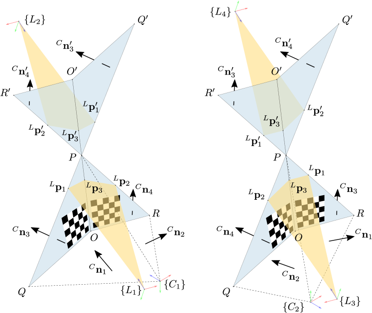
STEP 7: We must choose the unique solution from invalid solutions through the cheirality check. Fig. 4 shows four possible real solutions, which are {L1,C1}subscript𝐿1subscript𝐶1\{L_{1},C_{1}\}, {L2,C1}subscript𝐿2subscript𝐶1\{L_{2},C_{1}\}, {L3,C2}subscript𝐿3subscript𝐶2\{L_{3},C_{2}\} and {L4,C2}subscript𝐿4subscript𝐶2\{L_{4},C_{2}\} in terms of a combination of the LRF frame and the camera frame.
Refer to caption
Figure 4: Four possible real solutions are shown as a combination of the LRF frame and the camera frame ({L1,C1}subscript𝐿1subscript𝐶1\{L_{1},C_{1}\}, {L2,C1}subscript𝐿2subscript𝐶1\{L_{2},C_{1}\}, {L3,C2}subscript𝐿3subscript𝐶2\{L_{3},C_{2}\} and {L4,C2}subscript𝐿4subscript𝐶2\{L_{4},C_{2}\}). The unique solution {L1,C1}subscript𝐿1subscript𝐶1\{L_{1},C_{1}\} is determined through the cheirality check.

The unique solution {L1,C1}subscript𝐿1subscript𝐶1\{L_{1},C_{1}\} is determined as follows. Both the LRF and the camera must face towards the same direction, and three laser points 𝐩1Lsuperscriptsubscript𝐩1𝐿{{}^{L}}\mathbf{p}_{1}, 𝐩2Lsuperscriptsubscript𝐩2𝐿{{}^{L}}\mathbf{p}_{2} and 𝐩3Lsuperscriptsubscript𝐩3𝐿{{}^{L}}\mathbf{p}_{3} after transformation to the camera frame must be in front of the camera. These two conditions are

𝐧z𝐑L1C1𝐧z>0,𝐧z=[0,0,1]𝐧z(𝐑L1C1𝐩iL1+𝐭C1)L1>0,i={1,2,3}.\begin{gathered}\mathbf{n}_{z}^{\top}\cdot{{}_{L_{1}}^{C_{1}}}\mathbf{R}\cdot\mathbf{n}_{z}>0,\quad\mathbf{n}_{z}=[0,0,1]^{\top}\\ \mathbf{n}_{z}^{\top}\cdot\left({{}_{L_{1}}^{C_{1}}}\mathbf{R}\cdot{{}^{L_{1}}}\mathbf{p}_{i}+{{}^{C_{1}}}\mathbf{t}{{}_{L_{1}}}\right)>0,\quad i=\{1,2,3\}\end{gathered}. (31)

5.2 From Multiple Observations

Multiple observations from different views can be used to suppress noise. The problem in this case is formulated as follows

argmin𝐑LC,𝐭CLi=1Mj=1N(𝐧¯ijC(𝐑LC𝐩¯ijL+𝐭C)Ld¯ij)2s. t. 𝐑LC𝐑LC=𝐈,det(𝐑LC)=1,\begin{gathered}\operatornamewithlimits{argmin}_{{{}_{L}^{C}}\mathbf{R},{{}^{C}}\mathbf{t}{{}_{L}}}\sum_{i=1}^{M}\sum_{j=1}^{N}\left({{}^{C}}\bar{\mathbf{n}}_{ij}^{\top}\left({{}_{L}^{C}}\mathbf{R}\cdot{{}^{L}}\bar{\mathbf{p}}_{ij}+{{}^{C}}\mathbf{t}{{}_{L}}\right)-\bar{d}_{ij}\right)^{2}\\ \text{s. t. }\quad{{}_{L}^{C}}\mathbf{R}^{\top}\cdot{{}_{L}^{C}}\mathbf{R}=\mathbf{I},\quad\det\left({{}_{L}^{C}}\mathbf{R}\right)=1\end{gathered}, (32)

where N=6𝑁6N=6 and M𝑀M is the total number of different multiple observations. The solution is obtained through the seven steps mentioned in Subsection 5.1. As the rotation is represented by the Rodrigues’ formula, the calibration result is further refined using Levenberg-Marquardt (LM) method [21] [22]. Our solution in (32) serves as the accurate initial value.

6 Details of the Calibration Approach

We explain below how to accurately extract the features required for our method. These are four normal vectors 𝐧iCsuperscriptsubscript𝐧𝑖𝐶{{}^{C}}\mathbf{n}_{i} (i=1,2,3,4𝑖1234i=1,2,3,4) and two distances djsubscript𝑑𝑗d_{j} (j=1,2𝑗12j=1,2) from the camera, and three laser edge points 𝐩kLsuperscriptsubscript𝐩𝑘𝐿{{}^{L}}\mathbf{p}_{k} (k=1,2,3𝑘123k=1,2,3) from the LRF.

Refer to caption
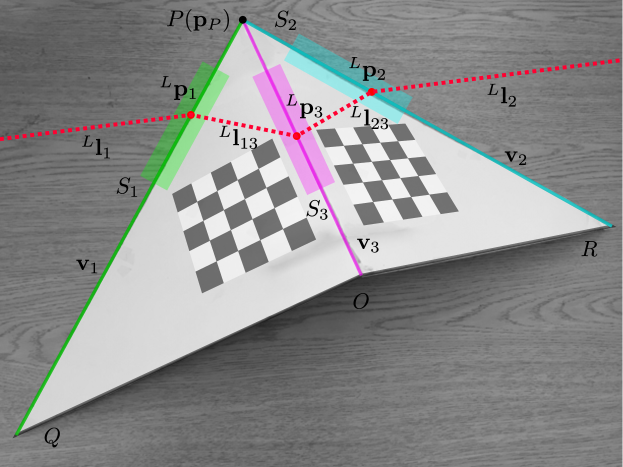
Figure 5: A calibration target built in a convex V-shape is put on the table. Accurate data extraction from both the LRF and the camera is performed by line intersection and optimized line detection.

6.1 Data from the LRF

Our calibration can be built in a convex shape as shown in Fig. 5. We can put the calibration target on a planar object (such as table, wall and the ground) such that 𝐩1Lsuperscriptsubscript𝐩1𝐿{{}^{L}}\mathbf{p}_{1}, 𝐩2Lsuperscriptsubscript𝐩2𝐿{{}^{L}}\mathbf{p}_{2} and 𝐩3Lsuperscriptsubscript𝐩3𝐿{{}^{L}}\mathbf{p}_{3} are accurately determined by the intersection between line segments. Specifically, the laser intersection with the objects are first segmented into four parts 𝐥1Lsuperscriptsubscript𝐥1𝐿{{}^{L}}\mathbf{l}_{1}, 𝐥13Lsuperscriptsubscript𝐥13𝐿{{}^{L}}\mathbf{l}_{13}, 𝐥23Lsuperscriptsubscript𝐥23𝐿{{}^{L}}\mathbf{l}_{23}, and 𝐥2Lsuperscriptsubscript𝐥2𝐿{{}^{L}}\mathbf{l}_{2} (e.g. using the Ramer-Douglas-Peucker algorithm (RDP) algorithm [23]). We then fit a line to each segment using the total least squares method [24]. 𝐩1Lsuperscriptsubscript𝐩1𝐿{{}^{L}}\mathbf{p}_{1} is thus obtained by the intersection of lines 𝐥1Lsuperscriptsubscript𝐥1𝐿{{}^{L}}\mathbf{l}_{1} and 𝐥13Lsuperscriptsubscript𝐥13𝐿{{}^{L}}\mathbf{l}_{13}. Similarly, 𝐩2Lsuperscriptsubscript𝐩2𝐿{{}^{L}}\mathbf{p}_{2} and 𝐩3Lsuperscriptsubscript𝐩3𝐿{{}^{L}}\mathbf{p}_{3} are respectively determined by the other two pairs {𝐥2L,𝐥23L}superscriptsubscript𝐥2𝐿superscriptsubscript𝐥23𝐿\{{{}^{L}}\mathbf{l}_{2},{{}^{L}}\mathbf{l}_{23}\} and {𝐥13L,𝐥23L}superscriptsubscript𝐥13𝐿superscriptsubscript𝐥23𝐿\{{{}^{L}}\mathbf{l}_{13},{{}^{L}}\mathbf{l}_{23}\}.

Refer to caption
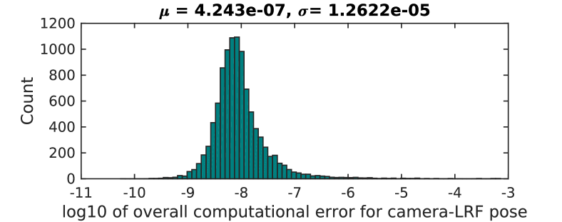
Figure 6: The histogram of computational errors for computed rotation and translation in 104superscript10410^{4} random and noise-free Monte-Carlo trials.

6.2 Data from the Camera

Using our calibration target with two checkerboards, the camera calibration is first performed by the MATLAB Toolbox [15]. Two normal vectors 𝐧3Csuperscriptsubscript𝐧3𝐶{{}^{C}}\mathbf{n}_{3} and 𝐧4Csuperscriptsubscript𝐧4𝐶{{}^{C}}\mathbf{n}_{4} of planes T3subscript𝑇3T_{3} and T4subscript𝑇4T_{4} can be obtained directly from the calibration toolbox. Each checkerboard is on the plane zT=0subscript𝑧𝑇0z_{T}=0 in its own world frame. For example, we have the rotation 𝐑T3Csubscriptsuperscript𝐑𝐶subscript𝑇3{{}_{T_{3}}^{C}}\mathbf{R} and translation 𝐭T3Csuperscriptsubscript𝐭subscript𝑇3𝐶{}^{C}\mathbf{t}_{T_{3}} from the calibration result, which represent the orientation and position of the plane T3subscript𝑇3T_{3} w.r.t. the camera. 𝐧3Csuperscriptsubscript𝐧3𝐶{{}^{C}}\mathbf{n}_{3} is just minus the 3rd column of 𝐑T3Csubscriptsuperscript𝐑𝐶subscript𝑇3{{}_{T_{3}}^{C}}\mathbf{R}, and the distance d1subscript𝑑1d_{1} from the camera to T3subscript𝑇3T_{3} is d1=𝐧3CC𝐭T3subscript𝑑1superscript𝐶superscriptsuperscriptsubscript𝐧3top𝐶subscript𝐭subscript𝑇3d_{1}={{}^{C}}\mathbf{n}_{3}^{\top}\cdot^{C}\mathbf{t}_{T_{3}}. Similarly, 𝐧4Csuperscriptsubscript𝐧4𝐶{{}^{C}}\mathbf{n}_{4} and d2subscript𝑑2d_{2} can be also calculated.

From the image (See Fig. 5), the unit line directions of PQ¯¯𝑃𝑄\overline{PQ}, PR¯¯𝑃𝑅\overline{PR} and PO¯¯𝑃𝑂\overline{PO} are projected as 𝐯1subscript𝐯1\mathbf{v}_{1}, 𝐯2subscript𝐯2\mathbf{v}_{2} and as 𝐯3subscript𝐯3\mathbf{v}_{3}, and the projection point of the vertex P𝑃P is 𝐩Psubscript𝐩𝑃\mathbf{p}_{P}. As stated in [13], we perform a weighted optimization initialized by the LSD [25] line detector to accurately estimate the set {𝐩P,𝐯1,𝐯2,𝐯3}subscript𝐩𝑃subscript𝐯1subscript𝐯2subscript𝐯3\{\mathbf{p}_{P},\mathbf{v}_{1},\mathbf{v}_{2},\mathbf{v}_{3}\}. Specifically, only the pixels within a rectangular region Sisubscript𝑆𝑖S_{i} are considered for fitting 𝐯isubscript𝐯𝑖\mathbf{v}_{i}. Let 𝜼isubscript𝜼𝑖\boldsymbol{\eta}_{i} be the normal of 𝐯isubscript𝐯𝑖\mathbf{v}_{i}. Hence, the optimization problem is expressed as

argmin𝐩P,𝐯1,𝐯2,𝐯3i=13j=1NiGij((𝐩ij𝐩P)𝜼i)2,subscriptargminsubscript𝐩𝑃subscript𝐯1subscript𝐯2subscript𝐯3superscriptsubscript𝑖13superscriptsubscript𝑗1subscript𝑁𝑖superscriptsubscript𝐺𝑖𝑗superscriptsuperscriptsubscript𝐩𝑖𝑗subscript𝐩𝑃subscript𝜼𝑖2\operatornamewithlimits{argmin}_{\mathbf{p}_{P},\mathbf{v}_{1},\mathbf{v}_{2},\mathbf{v}_{3}}\sum_{i=1}^{3}\sum_{j=1}^{N_{i}}G_{i}^{j}\cdot((\mathbf{p}_{i}^{j}-\mathbf{p}_{P})\cdot\boldsymbol{\eta}_{i})^{2}, (33)

where each region Sisubscript𝑆𝑖S_{i} has the number Nisubscript𝑁𝑖N_{i} of valid pixels 𝐩ijsuperscriptsubscript𝐩𝑖𝑗\mathbf{p}_{i}^{j} whose gradient magnitudes Gijsuperscriptsubscript𝐺𝑖𝑗G_{i}^{j} as their weights are above a threshold. Given the intrinsic matrix 𝐊𝐊\mathbf{K}, the normal vector 𝐧iCsuperscriptsubscript𝐧𝑖𝐶{{}^{C}}\mathbf{n}_{i} (i=1,2𝑖12i=1,2) is obtained by 𝐧iC=𝐊1𝐯i𝐊1𝐯isuperscriptsubscript𝐧𝑖𝐶superscript𝐊1subscript𝐯𝑖normsuperscript𝐊1subscript𝐯𝑖{{}^{C}}\mathbf{n}_{i}=\frac{\mathbf{K}^{-1}\mathbf{v}_{i}}{\|\mathbf{K}^{-1}\mathbf{v}_{i}\|}.

6.3 Snapshot Selection

The solution from a single snapshot constrains three laser points 𝐩kLsuperscriptsubscript𝐩𝑘𝐿{{}^{L}}\mathbf{p}_{k} (k=1,2,3𝑘123k=1,2,3). In the presence of noise, it should also guarantee that laser points 𝐩13iLsuperscriptsuperscriptsubscript𝐩13𝑖𝐿{{}^{L}}\mathbf{p}_{13}^{i} from the line 𝐥13Lsuperscriptsubscript𝐥13𝐿{{}^{L}}\mathbf{l}_{13} and 𝐩23jLsuperscriptsuperscriptsubscript𝐩23𝑗𝐿{{}^{L}}\mathbf{p}_{23}^{j} from 𝐥23Lsuperscriptsubscript𝐥23𝐿{{}^{L}}\mathbf{l}_{23} must respectively lie on T3subscript𝑇3T_{3} and T4subscript𝑇4T_{4}. We determine a snapshot as ill-conditioned if the average squared distance of laser points to their corresponding planes is larger than a threshold ϵ2superscriptitalic-ϵ2\epsilon^{2}. From multiple observations, it can guide us to select well-conditioned snapshots for further accuracy. Given the solution 𝐑^LCsubscriptsuperscript^𝐑𝐶𝐿{{}_{L}^{C}}\hat{\mathbf{R}} and 𝐭^CL{{}^{C}}\hat{\mathbf{t}}{{}_{L}}, we will keep this snapshot if it satisfies

i=1N13(𝐧3C(𝐑^LC𝐩13iL+𝐭^C)Ld1)22N13+j=1N23(𝐧4C(𝐑^LC𝐩23jL+𝐭^C)Ld2)22N23ϵ2,\scalebox{0.65}{$\sum\limits_{i=1}^{N_{13}}\dfrac{({{}^{C}}\mathbf{n}_{3}^{\top}({{}_{L}^{C}}\hat{\mathbf{R}}\cdot{{}^{L}}\mathbf{p}_{13}^{i}+{{}^{C}}\hat{\mathbf{t}}{{}_{L}})-d_{1})^{2}}{2N_{13}}+\sum\limits_{j=1}^{N_{23}}\dfrac{({{}^{C}}\mathbf{n}_{4}^{\top}({{}_{L}^{C}}\hat{\mathbf{R}}\cdot{{}^{L}}\mathbf{p}_{23}^{j}+{{}^{C}}\hat{\mathbf{t}}{{}_{L}})-d_{2})^{2}}{2N_{23}}\leq\epsilon^{2}$}, (34)

where 𝐥13Lsuperscriptsubscript𝐥13𝐿{{}^{L}}\mathbf{l}_{13} and 𝐥23Lsuperscriptsubscript𝐥23𝐿{{}^{L}}\mathbf{l}_{23} are treated equally, and have N13subscript𝑁13N_{13} and N23subscript𝑁23N_{23} points, respectively. The average squared distance of each line is first calculated and then half weighted as the left two terms of summation in Eq. (34).

7 Synthetic Experiments
Refer to caption
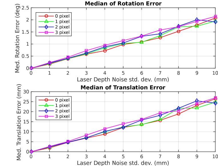
Figure 7: Errors in estimated rotation and translation as a function of the laser noise with different levels of the pixel noise. Each point represents the median error for 1000 Monte-Carlo trials. Each line corresponds to a different level of the pixel noise versus the laser noise changed by their own STDs.
Refer to caption
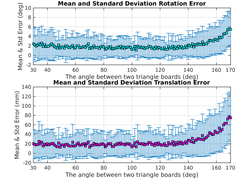
Figure 8: Means and STDs of the errors for estimated rotation and translation versus the angle between two triangle boards of the calibration target. Each point represents the mean error with its STD from 1000 Monte-Carlo trials. The errors gently vary as long as the angle between boards is obtuse.
Refer to caption
Figure 9: Means and STDs of the errors for estimated rotation and translation versus the number of observations of the calibration target in 1000 Monte-Carlo trials with the laser noise changed by its STD.
Refer to caption
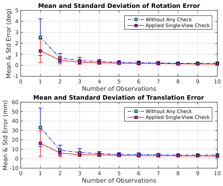
Figure 10: The comparision of means and STDs of the errors for estimated rotation and translation between single-view-check and without-any-check versus the number of observations of the calibration target in 1000 Monte-Carlo trials.

For the simulation setting, the obtuse angle between two triangle boards of the calibration target is set to 150superscript150150^{\circ}. Then, we uniformly and randomly generate roll, pitch and yaw in the range of ±45plus-or-minussuperscript45\pm 45^{\circ} for the orientation of the LRF w.r.t. the camera, and three components of the position from 5 to 30 cm. For each instance of the ground truth, we randomly generate the orientation and position of the calibration target within the range of ±45plus-or-minussuperscript45\pm 45^{\circ} and 50 to 150 cm. In the extreme case, the position angle between the LRF-to-target direction and the camera-to-target direction is more than 33superscript3333^{\circ}. It includes the scenario in proportion that the camera-to-LRF distance is large, as long as the target is visible from two sensors.

7.1 Numerical Stability

We performed 104superscript10410^{4} Monte-Carlo trials to validate the numerical stability of our solution in the noise-free case. For each trial, only one snapshot of the calibration target is needed. The error metric e=[𝐑gt|𝐭gt][𝐑^|𝐭^]e=\|[\mathbf{R}_{gt}|\mathbf{t}_{gt}]-[\hat{\mathbf{R}}|\hat{\mathbf{t}}]\|_{\mathcal{F}} is the Frobenius norm (\mathcal{F}) of the difference between the ground truth (gt𝑔𝑡gt) and our solution. The histogram of errors is shown in Fig. 6. The computational error varies but the accuracy is still high (around 108superscript10810^{-8}). It demonstrates that our method correctly solves the LRF-camera calibration problem, which further validates the sufficiency of the constraints from a single snapshot.

Refer to caption
Figure 11: Comparisons with the method of Zhang and Pless [5] and the method of Kwak et al. [10]. 1st and 2nd: Means of estimated rotation and translation errors for all three methods as the number of observations of the calibration target increases; 3rd and 4th: STDs of estimated rotation and translation errors for all three methods as the number of observations increases.

7.2 Sensitivity to Data Noise

This simulation tests the sensitivity of our solution to the noise in feature data. Two sources of error are taken into account: the laser depth uncertainty along the beam direction and the pixel uncertainty in line detection. Based on the practical setting, we respectively set the standard deviations (STDs) of laser noise and pixel error as σ1=10subscript𝜎110\sigma_{1}=10 mm and σ2=3subscript𝜎23\sigma_{2}=3 px in the 640×480640480640\times 480 image. A factor kσsubscript𝑘𝜎k_{\sigma} varies from 0 to 1 to combine the noise information as kσσisubscript𝑘𝜎subscript𝜎𝑖k_{\sigma}\sigma_{i} (i=1,2𝑖12i=1,2[13] from both sensors in one plot. 1000 Monte-Carlo trials are performed, each of which needs only one snapshot. The metrics for angular error (the chordal distance [26] of rotation) and distance error (translation) are respectively eθ=2arcsin(122𝐑^𝐑gt)subscript𝑒𝜃2122subscriptnorm^𝐑subscript𝐑𝑔𝑡e_{\theta}=2\arcsin(\frac{1}{2\sqrt{2}}\|\hat{\mathbf{R}}-\mathbf{R}_{gt}\|_{\mathcal{F}}) and ed=𝐭^𝐭gt2subscript𝑒𝑑subscriptnorm^𝐭subscript𝐭𝑔𝑡2e_{d}=\|\hat{\mathbf{t}}-\mathbf{t}_{gt}\|_{2}. Fig. 8 demonstrates that as the noise level increases, our solution is robust to the image noise but has a greater sensitivity to the laser depth noise.

7.3 Sensitivity to Angle between Boards

The sensitivity of our solution to the angle between two triangle boards of the calibration target is tested. We set σ1=10subscript𝜎110\sigma_{1}=10 mm and σ2=3subscript𝜎23\sigma_{2}=3 px. The angle varies from 30superscript3030^{\circ} to 170superscript170170^{\circ}. Fig. 8 shows the means and STDs for both angular and distance error. Our solution is not sensitive to the angle between boards but still has the smallest errors around 135superscript135135^{\circ}.

7.4 Noise Reduction

We report a simulation designed for testing the noise reduction of our solution when using multiple observations. Here, σ1subscript𝜎1\sigma_{1} varies from 1 mm to 10 mm with σ2subscript𝜎2\sigma_{2} set to 3 px. At each noise level, the means and STDs are calculated for both eθsubscript𝑒𝜃e_{\theta} and edsubscript𝑒𝑑e_{d} from 1000 Monte-Carlo trials. From Fig. 10, we observe that as number of observations increases, the means and STDs of both errors asymptotically decrease. Moreover, with a small number of snapshots, our solution can achieve a highly accurate initial value for further optimization. Specifically, eθsubscript𝑒𝜃e_{\theta} and edsubscript𝑒𝑑e_{d} are respectively around 0.5superscript0.50.5^{\circ} and 5 mm for only 5 snapshots.

7.5 Snapshot Selection

With snapshot selection, additional accuracy is achieved (See Fig. 10) in the presence of noise σ1=10subscript𝜎110\sigma_{1}=10 mm and σ2=3subscript𝜎23\sigma_{2}=3 px. The distance threshold ϵitalic-ϵ\epsilon is set to 5 mm. The errors eθsubscript𝑒𝜃e_{\theta} and edsubscript𝑒𝑑e_{d} are further decreased by nearly 50%percent5050\% compared with the solution without any single-snapshot check. Specifically, eθsubscript𝑒𝜃e_{\theta} and edsubscript𝑒𝑑e_{d} are respectively around 0.25superscript0.250.25^{\circ} and 2 mm for only 5 snapshots. Thus, our method can guarantee a high accuracy of the solution when using multiple snapshots.

8 Real Experiments

To further validate our method, we perform real experiments in comparison with other two existing methods [5] and [10].

A LRF Hokuyo URG-04LX is rigidly mounted on a stereo rig which consists of a pair of Point Grey Chameleon CMLN-13S2C cameras (See Fig. 1). Sensors are synchronized based on time stamps. The LRF is set to 180superscript180180^{\circ} horizontal field of view, with an angular resolution of 0.36superscript0.360.36^{\circ} and a line scanning frequency of 10 Hz. Its scanning accuracy is ±1plus-or-minus1\pm 1 cm within a range from 2 cm to 100 cm, and has 1%percent11\% error for a range from 100 cm to 400 cm. The cameras have a resolution of 640×480640480640\times 480 pixels, and are pre-calibrated based on [28]. The images prior to data processing are warped to get rid off the radial and tangent distortions.

8.1 Comparison with Existing Methods

We compare our method to two state-of-the-art algorithms [5] and [10] using the ground truth of the stereo-rig baseline. Specifically, let 𝐓=[𝐑𝐭0001]𝐓delimited-[]𝐑𝐭0001\mathbf{T}=\left[\begin{smallmatrix}\mathbf{R}&\mathbf{t}\\ 000&1\end{smallmatrix}\right] represent the transformation (rotation and translation) between two frames. For each method, the LRF is first calibrated w.r.t both left and right cameras to obtain 𝐓LClsubscriptsuperscript𝐓subscript𝐶𝑙𝐿{}_{L}^{C_{l}}\mathbf{T} and 𝐓LCrsubscriptsuperscript𝐓subscript𝐶𝑟𝐿{}_{L}^{C_{r}}\mathbf{T}. We then compute the relative pose (baseline) between stereo cameras and compare it with the the ground truth 𝐓ClCrsubscriptsuperscript𝐓subscript𝐶𝑟subscript𝐶𝑙{}_{C_{l}}^{C_{r}}\mathbf{T} calibrated from the toolbox [15]. Hence, the error matrix is 𝐓e=ClCr𝐓LCl𝐓(LCr𝐓)1\mathbf{T}_{e}=_{C_{l}}^{C_{r}}\mathbf{T}\cdot_{L}^{C_{l}}\mathbf{T}\cdot(_{L}^{C_{r}}\mathbf{T})^{-1}, where 𝐑esubscript𝐑𝑒\mathbf{R}_{e} and 𝐭e2subscriptnormsubscript𝐭𝑒2\|\mathbf{t}_{e}\|_{2} are respectively compared with the identity and zero.

The stereo cameras are calibrated for 10 times where each time 20 image pairs are randomly chosen from 40 pairs. With the rotation represented by the Rodrigues’ formula, the means of the rotation angle and the baseline distance are respectively 0.0137superscript0.01370.0137^{\circ} and 96.0511 mm (the translation is [96.050596.0505-96.0505, 0.30350.3035-0.3035, 0.13260.1326-0.1326] in mm). Because of their low STDs 0.0018superscript0.00180.0018^{\circ} and 0.2742 mm (within 0.01superscript0.010.01^{\circ} and 1 mm), we treat their means as the ground truth. The distances between the LRF and the stereo cameras are approximately 100 mm and 150 mm. 30 best observations of each method are obtained using a RANSAC framework (5 snapshots are randomly chosen from a total 50). We randomly select subsets of 1, 5, 10, 15 and 20 observations to perform the calibration between the LRF and the stereo rig. The calibration is performed 10 times for each random subset.

Fig. 11 shows that our method has the smallest errors of both rotation and translation as the number of observations increases. Specifically, the mean errors from 20 observations are respectively 0.3superscript0.30.3^{\circ} and 3.43.43.4 mm almost three times lower than the method of Zhang and Pless (1.3superscript1.31.3^{\circ} and 12.012.012.0 mm) and the method of Kwak et al. (1.0superscript1.01.0^{\circ} and 12.612.612.6 mm). Moreover, our method can obtain a reasonable result even using only one snapshot, which is not possible for the other two methods. In other words, our method can achieve an accuracy at the same level but using the smallest number of observations.

8.2 Real Scene Validation

This experiment from the real scene tests the calibration results between LRF to both left and right cameras, respectively, obtained by two existing methods [5] [10] and our method for comparison (See Fig. 12). We generate a dataset of 30 input observations for each method using their own calibration targets. The calibration results are obtained from 20 observations randomly chosen from 30 in total of each method. We then respectively test them using the stereo images from new observations of our calibration target which are not involved in the calibration process. From the comparison, we observe that the laser scanning lines for our method more reasonably match the calibration target (board boundaries) from both left and right cameras. Thus, it validates the correctness of our calibration results of each LRF-camera pair.
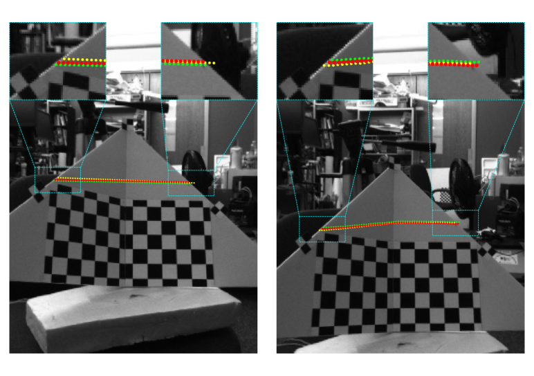
Refer to caption
Figure 12: The projection of laser points scanned on the calibration target onto the images from both left and right cameras using three different methods. Cyan boxes show the close-up of laser point projection. Methods [5] and [10] are green and yellow colored, respectively. Our approach is red colored.

9 Conclusion

In this paper, we presented a novel method for calibrating the extrinsic parameters of a system of a camera and a 2D laser rangefinder. In contrast to existing methods, our coplanarity constraints for feature data suffice to unambiguously determine the relative pose between these two sensors even from a single observation. A series of experiments verified that the number of observations can be drastically reduced for an accurate result. Our solution technique was also extended to the case of multiple observations to reduce noise for further refinement. We are working on releasing our code [29].

Appendix A Proof of Lemma 1

From Fig. 2, 𝐧iCsuperscriptsubscript𝐧𝑖𝐶{{}^{C}}\mathbf{n}_{i} is the normal vector of plane Tisubscript𝑇𝑖T_{i} for i=1,2,3,4𝑖1234i={1,2,3,4} and we claim that these normal vectors in any cardinality three subset of {𝐧1C,𝐧2C,𝐧3C,𝐧4C}superscriptsubscript𝐧1𝐶superscriptsubscript𝐧2𝐶superscriptsubscript𝐧3𝐶superscriptsubscript𝐧4𝐶\{{{}^{C}}\mathbf{n}_{1},{{}^{C}}\mathbf{n}_{2},{{}^{C}}\mathbf{n}_{3},{{}^{C}}\mathbf{n}_{4}\} are linearly independent. It is obvious that there are totally four subsets: I. 𝐧1Csuperscriptsubscript𝐧1𝐶{{}^{C}}\mathbf{n}_{1}, 𝐧2Csuperscriptsubscript𝐧2𝐶{{}^{C}}\mathbf{n}_{2} and 𝐧3Csuperscriptsubscript𝐧3𝐶{{}^{C}}\mathbf{n}_{3}; II. 𝐧1Csuperscriptsubscript𝐧1𝐶{{}^{C}}\mathbf{n}_{1}, 𝐧2Csuperscriptsubscript𝐧2𝐶{{}^{C}}\mathbf{n}_{2} and 𝐧4Csuperscriptsubscript𝐧4𝐶{{}^{C}}\mathbf{n}_{4}; III. 𝐧1Csuperscriptsubscript𝐧1𝐶{{}^{C}}\mathbf{n}_{1}, 𝐧3Csuperscriptsubscript𝐧3𝐶{{}^{C}}\mathbf{n}_{3} and 𝐧4Csuperscriptsubscript𝐧4𝐶{{}^{C}}\mathbf{n}_{4}; IV. 𝐧2Csuperscriptsubscript𝐧2𝐶{{}^{C}}\mathbf{n}_{2}, 𝐧3Csuperscriptsubscript𝐧3𝐶{{}^{C}}\mathbf{n}_{3} and 𝐧4Csuperscriptsubscript𝐧4𝐶{{}^{C}}\mathbf{n}_{4}. We will prove separately for each subset and show that subsets I and II are symmetric arguments, and subsets III and IV are also symmetric arguments.

According to the geometry setting in Fig. 2, we notice that for each subset three different planes have a common intersection point P𝑃P, which means there is no parallelism between them. We let 𝐥12subscript𝐥12\mathbf{l}_{12}, 𝐥13subscript𝐥13\mathbf{l}_{13}, 𝐥23subscript𝐥23\mathbf{l}_{23} and 𝐥34subscript𝐥34\mathbf{l}_{34} respectively denote the directional unit vectors of the lines PC¯¯𝑃𝐶\overline{PC}, PQ¯¯𝑃𝑄\overline{PQ}, PR¯¯𝑃𝑅\overline{PR} and PO¯¯𝑃𝑂\overline{PO} w.r.t. the camera frame.

So let us first prove the claim for subset I: 𝐧1Csuperscriptsubscript𝐧1𝐶{{}^{C}}\mathbf{n}_{1}, 𝐧2Csuperscriptsubscript𝐧2𝐶{{}^{C}}\mathbf{n}_{2} and 𝐧3Csuperscriptsubscript𝐧3𝐶{{}^{C}}\mathbf{n}_{3}. We assume that these three normal vectors are linearly dependent, which means there exists three nonzero coefficients α𝛼\alpha, β𝛽\beta and γ𝛾\gamma such that α𝐧1C+β𝐧2C+γ𝐧3C=0𝛼superscriptsubscript𝐧1𝐶𝛽superscriptsubscript𝐧2𝐶𝛾superscriptsubscript𝐧3𝐶0\alpha{{}^{C}}\mathbf{n}_{1}+\beta{{}^{C}}\mathbf{n}_{2}+\gamma{{}^{C}}\mathbf{n}_{3}=0, otherwise two of three planes would have parallelism (e.g. α=0𝛼0\alpha=0 such that β𝐧2C=γ𝐧3C𝛽superscriptsubscript𝐧2𝐶𝛾superscriptsubscript𝐧3𝐶\beta{{}^{C}}\mathbf{n}_{2}=-\gamma{{}^{C}}\mathbf{n}_{3}) or one plane of them reduces to nonexistence (e.g. α=β=0𝛼𝛽0\alpha=\beta=0 such that γ𝐧3C=0𝛾superscriptsubscript𝐧3𝐶0\gamma{{}^{C}}\mathbf{n}_{3}=0). Thus, 𝐧3Csuperscriptsubscript𝐧3𝐶{{}^{C}}\mathbf{n}_{3} can be represented as the combination of 𝐧1Csuperscriptsubscript𝐧1𝐶{{}^{C}}\mathbf{n}_{1} and 𝐧2Csuperscriptsubscript𝐧2𝐶{{}^{C}}\mathbf{n}_{2}. Since the intersecting line of T1subscript𝑇1T_{1} and T2subscript𝑇2T_{2} is PC¯¯𝑃𝐶\overline{PC}, we have the following

{𝐥12𝐧1C=0𝐥12𝐧2C=0𝐥12𝐧3C=0.casessuperscriptsubscript𝐥12topsuperscriptsubscript𝐧1𝐶0otherwisesuperscriptsubscript𝐥12topsuperscriptsubscript𝐧2𝐶0otherwisesuperscriptsubscript𝐥12topsuperscriptsubscript𝐧3𝐶0\begin{cases}\mathbf{l}_{12}^{\top}\cdot{{}^{C}}\mathbf{n}_{1}=0\\ \mathbf{l}_{12}^{\top}\cdot{{}^{C}}\mathbf{n}_{2}=0\end{cases}\quad\Rightarrow\quad\mathbf{l}_{12}^{\top}\cdot{{}^{C}}\mathbf{n}_{3}=0. (35)

It means that the line PC¯¯𝑃𝐶\overline{PC} is on the plane T3subscript𝑇3T_{3} given the fact that they share a common point P𝑃P. It is a contradiction unless camera center C𝐶C is also on the plane T3subscript𝑇3T_{3}, which is a useless case since camera cannot capture the checkerboard on T3subscript𝑇3T_{3}. Thus, the normal vectors 𝐧1Csuperscriptsubscript𝐧1𝐶{{}^{C}}\mathbf{n}_{1}, 𝐧2Csuperscriptsubscript𝐧2𝐶{{}^{C}}\mathbf{n}_{2} and 𝐧3Csuperscriptsubscript𝐧3𝐶{{}^{C}}\mathbf{n}_{3} are linearly independent. It is similar for subset II that we would have a contradiction that the line PC¯¯𝑃𝐶\overline{PC} is on the plane T4subscript𝑇4T_{4} based on 𝐥12𝐧4C=0superscriptsubscript𝐥12topsuperscriptsubscript𝐧4𝐶0\mathbf{l}_{12}^{\top}\cdot{{}^{C}}\mathbf{n}_{4}=0 if 𝐧1Csuperscriptsubscript𝐧1𝐶{{}^{C}}\mathbf{n}_{1}, 𝐧2Csuperscriptsubscript𝐧2𝐶{{}^{C}}\mathbf{n}_{2} and 𝐧4Csuperscriptsubscript𝐧4𝐶{{}^{C}}\mathbf{n}_{4} are linear dependent. So we can conclude that these vectors in both subset I and II are linearly independent.

Next let us focus on the claim for subset III: 𝐧1Csuperscriptsubscript𝐧1𝐶{{}^{C}}\mathbf{n}_{1}, 𝐧3Csuperscriptsubscript𝐧3𝐶{{}^{C}}\mathbf{n}_{3} and 𝐧4Csuperscriptsubscript𝐧4𝐶{{}^{C}}\mathbf{n}_{4}. We assume that these three normal vectors are linearly dependent, which means there exists three nonzero coefficients α𝛼\alpha, β𝛽\beta and γ𝛾\gamma as explained in subset I such that α𝐧1C+β𝐧3C+γ𝐧4C=0𝛼superscriptsubscript𝐧1𝐶𝛽superscriptsubscript𝐧3𝐶𝛾superscriptsubscript𝐧4𝐶0\alpha{{}^{C}}\mathbf{n}_{1}+\beta{{}^{C}}\mathbf{n}_{3}+\gamma{{}^{C}}\mathbf{n}_{4}=0. Thus, 𝐧1Csuperscriptsubscript𝐧1𝐶{{}^{C}}\mathbf{n}_{1} can be represented as the combination of 𝐧3Csuperscriptsubscript𝐧3𝐶{{}^{C}}\mathbf{n}_{3} and 𝐧4Csuperscriptsubscript𝐧4𝐶{{}^{C}}\mathbf{n}_{4}. Since the intersecting line of T3subscript𝑇3T_{3} and T4subscript𝑇4T_{4} is PO¯¯𝑃𝑂\overline{PO}, we have the following

{𝐥34𝐧3C=0𝐥34𝐧4C=0𝐥34𝐧1C=0.casessuperscriptsubscript𝐥34topsuperscriptsubscript𝐧3𝐶0otherwisesuperscriptsubscript𝐥34topsuperscriptsubscript𝐧4𝐶0otherwisesuperscriptsubscript𝐥34topsuperscriptsubscript𝐧1𝐶0\begin{cases}\mathbf{l}_{34}^{\top}\cdot{{}^{C}}\mathbf{n}_{3}=0\\ \mathbf{l}_{34}^{\top}\cdot{{}^{C}}\mathbf{n}_{4}=0\end{cases}\quad\Rightarrow\quad\mathbf{l}_{34}^{\top}\cdot{{}^{C}}\mathbf{n}_{1}=0. (36)

It means that the line PO¯¯𝑃𝑂\overline{PO} is on the plane T1subscript𝑇1T_{1} given the fact that they share a common point P𝑃P. It is a contradiction unless the corner O𝑂O of the calibration target is also on the plane T1subscript𝑇1T_{1}, which is a useless case since camera cannot capture the checkerboard on T3subscript𝑇3T_{3}. Thus, the normal vectors 𝐧1Csuperscriptsubscript𝐧1𝐶{{}^{C}}\mathbf{n}_{1}, 𝐧3Csuperscriptsubscript𝐧3𝐶{{}^{C}}\mathbf{n}_{3} and 𝐧4Csuperscriptsubscript𝐧4𝐶{{}^{C}}\mathbf{n}_{4} are linearly independent. It is similar for subset IV that we would have a contradiction that the line PO¯¯𝑃𝑂\overline{PO} is on the plane T2subscript𝑇2T_{2} based on 𝐥34𝐧2C=0superscriptsubscript𝐥34topsuperscriptsubscript𝐧2𝐶0\mathbf{l}_{34}^{\top}\cdot{{}^{C}}\mathbf{n}_{2}=0 if 𝐧2Csuperscriptsubscript𝐧2𝐶{{}^{C}}\mathbf{n}_{2}, 𝐧3Csuperscriptsubscript𝐧3𝐶{{}^{C}}\mathbf{n}_{3} and 𝐧4Csuperscriptsubscript𝐧4𝐶{{}^{C}}\mathbf{n}_{4} are linear dependent. So we can conclude that these vectors in both subset III and IV are also linearly independent.

Above all, it is proved that three normal vectors in each subset from I, II, III and IV are linearly independent. \blacksquare

Appendix B Proof of Lemma 2

From Appendix A, we know that any three of normal vectors 𝐧1Csuperscriptsubscript𝐧1𝐶{{}^{C}}\mathbf{n}_{1}, 𝐧2Csuperscriptsubscript𝐧2𝐶{{}^{C}}\mathbf{n}_{2}, 𝐧3Csuperscriptsubscript𝐧3𝐶{{}^{C}}\mathbf{n}_{3} and 𝐧4Csuperscriptsubscript𝐧4𝐶{{}^{C}}\mathbf{n}_{4} can span the whole 3D space. Based on the definitions in (13), the matrix in (15) is

𝒩o=i=1N𝐧¯iC𝐧¯iC=𝐧1C𝐧1C+𝐧2C𝐧2C+2𝐧3C𝐧3C+2𝐧4C𝐧4C,subscript𝒩𝑜superscriptsubscript𝑖1𝑁superscriptsubscript¯𝐧𝑖𝐶superscriptsuperscriptsubscript¯𝐧𝑖top𝐶superscriptsubscript𝐧1𝐶superscriptsuperscriptsubscript𝐧1top𝐶superscriptsubscript𝐧2𝐶superscriptsuperscriptsubscript𝐧2top𝐶2superscriptsubscript𝐧3𝐶superscriptsuperscriptsubscript𝐧3top𝐶2superscriptsubscript𝐧4𝐶superscriptsuperscriptsubscript𝐧4top𝐶\scalebox{0.75}{$\mathcal{N}_{o}=\sum_{i=1}^{N}{{}^{C}}\bar{\mathbf{n}}_{i}{{}^{C}}\bar{\mathbf{n}}_{i}^{\top}={{}^{C}}\mathbf{n}_{1}{{}^{C}}\mathbf{n}_{1}^{\top}+{{}^{C}}\mathbf{n}_{2}{{}^{C}}\mathbf{n}_{2}^{\top}+2{{}^{C}}\mathbf{n}_{3}{{}^{C}}\mathbf{n}_{3}^{\top}+2{{}^{C}}\mathbf{n}_{4}{{}^{C}}\mathbf{n}_{4}^{\top}$}, (37)

which is a symmetric matrix. We now show that this matrix is non-singular.

As is known, the eigenvalues of a positive definite matrix are all positive [30]. Further, we know that a positive definite matrix is always invertible [30]. From the properties above, we just need to prove that 𝒩osubscript𝒩𝑜\mathcal{N}_{o} is positive definite. Let 𝐯𝟎𝐯0\mathbf{v}\neq\mathbf{0} be an arbitrary non-zero vector. Then we calculate the quadratic form

𝐯𝒩o𝐯=(𝐧1C𝐯)2+(𝐧2C𝐯)2+2(𝐧3C𝐯)2+2(𝐧4C𝐯)20.𝐯𝒩o𝐯=(𝐧1C𝐯)2+(𝐧2C𝐯)2+2(𝐧3C𝐯)2+2(𝐧4C𝐯)20\scalebox{0.8}{$\mathbf{v}^{\top}\mathcal{N}_{o}\mathbf{v}=\left({{}^{C}}\mathbf{n}_{1}^{\top}\mathbf{v}\right)^{2}+\left({{}^{C}}\mathbf{n}_{2}^{\top}\mathbf{v}\right)^{2}+2\left({{}^{C}}\mathbf{n}_{3}^{\top}\mathbf{v}\right)^{2}+2\left({{}^{C}}\mathbf{n}_{4}^{\top}\mathbf{v}\right)^{2}\geq 0$}. (38)

We assume that 𝐯𝒩o𝐯=0superscript𝐯topsubscript𝒩𝑜𝐯0\mathbf{v}^{\top}\mathcal{N}_{o}\mathbf{v}=0, which means 𝐧iC𝐯=0superscriptsuperscriptsubscript𝐧𝑖top𝐶𝐯0{{}^{C}}\mathbf{n}_{i}^{\top}\mathbf{v}=0 for i={1,2,3,4}𝑖1234i=\{1,2,3,4\}. However, since any three of these four normal vectors are linearly independent, we get a contradiction that, for example, [𝐧1C,𝐧2C,𝐧3C]𝐯=𝟎superscriptsuperscriptsubscript𝐧1𝐶superscriptsubscript𝐧2𝐶superscriptsubscript𝐧3𝐶top𝐯0[{{}^{C}}\mathbf{n}_{1},{{}^{C}}\mathbf{n}_{2},{{}^{C}}\mathbf{n}_{3}]^{\top}\mathbf{v}=\mathbf{0} if and only if 𝐯=𝟎𝐯0\mathbf{v}=\mathbf{0}. Thus, we can conclude that

𝐯𝒩o𝐯=(𝐧1C𝐯)2+(𝐧2C𝐯)2+2(𝐧3C𝐯)2+2(𝐧4C𝐯)2>0.superscript𝐯topsubscript𝒩𝑜𝐯superscriptsuperscriptsuperscriptsubscript𝐧1top𝐶𝐯2superscriptsuperscriptsuperscriptsubscript𝐧2top𝐶𝐯22superscriptsuperscriptsuperscriptsubscript𝐧3top𝐶𝐯22superscriptsuperscriptsuperscriptsubscript𝐧4top𝐶𝐯20\scalebox{0.8}{$\mathbf{v}^{\top}\mathcal{N}_{o}\mathbf{v}=\left({{}^{C}}\mathbf{n}_{1}^{\top}\mathbf{v}\right)^{2}+\left({{}^{C}}\mathbf{n}_{2}^{\top}\mathbf{v}\right)^{2}+2\left({{}^{C}}\mathbf{n}_{3}^{\top}\mathbf{v}\right)^{2}+2\left({{}^{C}}\mathbf{n}_{4}^{\top}\mathbf{v}\right)^{2}>0$}. (39)

Thus, matrix 𝒩osubscript𝒩𝑜\mathcal{N}_{o} is positive definite and always invertible. \blacksquare

References

  • [1] B. Douillard, D. Fox, F. Ramos, and H. Durrant-Whyte, “Classification and semantic mapping of urban environments,” in The international journal of robotics research, vol. 30, no. 1, pp. 5-32, 2011.
  • [2] S. A. Rodriguez, V. Fremont, and P. Bonnifait, “Extrinsic calibration between a multi-layer lidar and a camera,” in IEEE Int. Conf. on Multisensor Fusion and Integration for Intelligent Systems, vol. 1, pp. 214-219, Seoul, Korea, 2008.
  • [3] X. Gong, Y. Lin, and J. Liu, “3D LIDAR-camera extrinsic calibration using an arbitrary trihedron,” Sensors, vol. 13, no. 2, pp. 1902-1918, 2013.
  • [4] V. Lepetit, F. Moreno-Noguer, and P. Fua, “Epnp: An accurate o(n) solution to the pnp problem,” International Journal of Computer Vision, vol. 81, pp. 155-166, February 2009.
  • [5] Q. Zhang and R. Pless, “Extrinsic calibration of a camera and laser range finder (improves camera calibration),” in IEEE/RSJ International Conference on Intelligent Robots and Systems (IROS’04), vol. 3, pp. 2301-2306, 2004.
  • [6] F. Vasconcelos, J. P. Barreto, and U. Nunes, “A minimal solution for the extrinsic calibration of a camera and a laser-rangefinder,” IEEE Transactions on Pattern Analysis and Machine Intelligence (PAMI), vol. 34, no. 11, pp. 2097-2107, 2012.
  • [7] L. Zhou, “A new minimal solution for the extrinsic calibration of a 2d lidar and a camera using three plane-line correspondences,” in IEEE Sensors Journal, vol. 14, no. 2, pp. 442-454, 2014.
  • [8] G. Li, Y. Liu, L. Dong, X. Cai, and D. Zhou, “An algorithm for extrinsic parameters calibration of a camera and a laser range finder using line features,” in Proceedings of the IEEE/RSJ International Conference on Intelligent Robots and Systems (IROS), pp. 3854-3859, 2007.
  • [9] S. Wasielewski and O. Strauss, “Calibration of a multi-sensor system laser rangefinder/camera,” in IEEE Proc. of the Intelligent Vehicles ’95 Symposium, pp. 472-477, 1995.
  • [10] K. Kwak, D. F. Huber, H. Badino, and T. Kanade, “Extrinsic calibration of a single line scanning lidar and a camera,” IEEE Proceedings of International Conference on Intelligent Robots and Systems (IROS), pp. 3283-3289, 2011.
  • [11] O. Naroditsky, A. Patterson, and K. Daniilidis, “Automatic alignment of a camera with a line scan lidar system,” in Proc. of the IEEE International Conference on Robotics and Automation (ICRA), pp. 3429-3434, 2011.
  • [12] C. X. Guo and S. I. Roumeliotis, “An analytical least-squares solution to the line scan LIDAR-camera extrinsic calibration problem,” in Proc. of the IEEE International Conference on Robotics and Automation (ICRA), pp. 2943-2948, Karlsruhe, Germany, 2013.
  • [13] R. Gomez-Ojeda, J. Briales, E. Fernández-Moral, and J. Gonzalez-Jimenez, “Extrinsic calibration of a 2D laser-rangefinder and a camera based on scene corners,” in IEEE International Conference on Robotics and Automation (ICRA), Seattle, USA, 2015.
  • [14] Z. Hu, Y. Li, N. Li, and B. Zhao, “Extrinsic calibration of 2-D laser rangefinder and camera from single shot based on minimal solution,” in IEEE Transactions on Instrumentation and Measurement, vol. 65, no. 4, pp. 915-929, 2016.
  • [15] J.-Y. Bouguet, “Camera calibration toolbox for matlab,” 2004.
  • [16] P. F. Stiller, “An introduction to the theory of resultants,” 1996.
  • [17] A. Edelman, and H. Murakami, “Polynomial roots from companion matrix eigenvalues,” Mathematics of Computation, vol. 64, no. 210, pp. 763-776, 1995.
  • [18] S. Fortune, “An iterated eigenvalue algorithm for approximating roots of univariate polynomials,” Journal of Symbolic Computation, vol. 33, no. 5, pp. 627-646, 2002.
  • [19] A. R. Conn, N. IM. Gould, and P. L. Toint, “Trust region methods,” Society for Industrial and Applied Mathematics, 2000.
  • [20] M. JD. Powell, “A Fortran subroutine for solving systems for nonlinear algebraic equations,” Numerical methods for nonlinear algebraic equations, pp. 115-161, 1970.
  • [21] K. Levenberg, “A method for the solution of certain non-linear problems in least squares,” Quarterly of Applied Mathematics, vol. 2, pp. 164-168, 1944.
  • [22] D. W. Marquardt, “An algorithm for least-squares estimation of nonlinear parameters,” Journal of the society for Industrial and Applied Mathematics, vol. 11, no. 2, pp. 431-441, 1963.
  • [23] D. H. Douglas, and T. K. Peucker, “Algorithms for the reduction of the number of points required to represent a digitized line or its caricature,” Cartographica: The International Journal for Geographic Information and Geovisualization, vol. 10, no. 2, pp. 112-122, 1973.
  • [24] G. H. Golub and C. F. Van Loan, “An analysis of the total least squares problem,” SIAM Journal on Numerical Analysis, vol. 17, pp. 883-893, 1980.
  • [25] V. Gioi, J. Jakubowicz, J. Morel, and G. Rafael, “LSD: A fast line segment detector with a false detection control,” IEEE transactions on pattern analysis and machine intelligence, vol. 32, no. 4, pp. 722-732, 2010.
  • [26] R. Hartley, J. Trumpf, Y. Dai, and H. Li. “Rotation averaging,” International Journal of Computer Vision, vol. 103, no. 3, pp. 267-305, 2013.
  • [27] W. Dong, and V. Isler, “A novel method for the extrinsic calibration of a 2-D laser-rangefinder & a camera,” Robotics and Automation (ICRA), 2017 IEEE International Conference on, pp. 5104-5109, 2017.
  • [28] Z. Zhang, “A flexible new technique for camera calibration,” IEEE Trans. Pattern Analysis and Machine Intelligence, vol. 22, no. 11, pp. 1330-1334, 2000.
  • [29] http://rsn.cs.umn.edu/index.php/Downloads
  • [30] C. R. Johnson, “Positive definite matrices,” The American Mathematical Monthly, vol. 77, no. 3, pp. 259-264, 1970.
{biography}

Wenbo Dong is a PhD student in the Department of Computer Science and Engineering at the University of Minnesota, Twin Cities. He obtained his MS degree (2017) in Computer Science at the University of Minnesota. He obtained his BE (2012) and ME (2014) degrees in Electrical Engineering at Harbin Institute of Technology, Harbin, China. His research interests include robotics, 3D computer vision and their applications in precision agriculture.

{biography}

Volkan Isler is a Professor in the Department of Computer Science and Engineering at the University of Minnesota. He obtained his MSE (2000) and PhD (2004) degrees in Computer and Information Science from the University of Pennsylvania. He obtained his BS degree (1999) in Computer Engineering from Bogazici University, Istanbul, Turkey. In 2008, he received the National Science Foundation’s Young Investigator Award (CAREER). From 2009 to 2015, he chaired IEEE Society of Robotics and Automation’s Technical Committee on Networked Robots. He also served as an Associate Editor for IEEE Transactions on Robotics and IEEE Transactions on Automation Science and Engineering. He is currently an Editor for the ICRA Editorial Board. His research interests are primarily in robotics, computer vision, sensor networks and geometric algorithms, and their applications in agriculture and environmental monitoring.