Optimal Event-Driven Multi-Agent Persistent Monitoring of a Finite Set of Targets

Nan Zhou1, Xi Yu2, Sean B. Andersson1,2, and Christos G. Cassandras1,3
1Division of Systems Engineering, 2Department of Mechanical Engineering , 3Department of Electrical and Computer Engineering
Boston University, Boston, MA 02215, USA
E-mail:{nanzhou,xyu,sanderss,cgc}@bu.edu
* The work of Cassandras and Zhou is supported in part by NSF under grants CNS-1239021, ECCS-1509084, and IIP-1430145, by AFOSR under grant FA9550-15-1-0471, and by ONR under grant N00014-09-1-1051. The work of Andersson and Yu is supported in part by the NSF through grant ECCS-1509084.
Abstract

We consider the problem of controlling the movement of multiple cooperating agents so as to minimize an uncertainty metric associated with a finite number of targets. In a one-dimensional mission space, we adopt an optimal control framework and show that the solution is reduced to a simpler parametric optimization problem: determining a sequence of locations where each agent may dwell for a finite amount of time and then switch direction. This amounts to a hybrid system which we analyze using Infinitesimal Perturbation Analysis (IPA) to obtain a complete on-line solution through an event-driven gradient-based algorithm which is also robust with respect to the uncertainty model used. The resulting controller depends on observing the events required to excite the gradient-based algorithm, which cannot be guaranteed. We solve this problem by proposing a new metric for the objective function which creates a potential field guaranteeing that gradient values are non-zero. This approach is compared to an alternative graph-based task scheduling algorithm for determining an optimal sequence of target visits. Simulation examples are included to demonstrate the proposed methods.

I Introduction

Systems consisting of cooperating mobile agents are often used to perform tasks such as coverage control [1, 2], surveillance, and environmental sampling. The persistent monitoring problem arises when agents must monitor a dynamically changing environment which cannot be fully covered by a stationary team of agents. Thus, persistent monitoring differs from traditional coverage tasks due to the perpetual need to cover a changing environment [3, 4]. A result of this exploration process is the eventual discovery of various “points of interest” which, once detected, become “targets” or “data sources” which need to be monitored. This setting arises in multiple application domains ranging from surveillance, environmental monitoring, and energy management [5, 6] down to nano-scale systems tasked to track fluorescent or magnetic particles for the study of dynamic processes in bio-molecular systems and in nano-medical research [7, 8]. In contrast to [3, 4] where every point in a mission space must be monitored, the problem we address here involves a finite number of targets (typically larger than the number of agents) which the agents must cooperatively monitor through periodic visits.

Each target may be viewed as a dynamic system in itself whose state is observed by agents equipped with sensing capabilities (e.g., cameras) and which are normally dependent upon their physical distance from the target. The objective of cooperative persistent monitoring in this case is to minimize an overall measure of uncertainty about the target states. This may be accomplished by assigning agents to specific targets or by designing motion trajectories through which agents reduce the uncertainty related to a target by periodically visiting it (and possibly remaining at the target for a finite amount of time). Viewed as an optimization problem, the goal is to jointly minimize some cost function that captures the desired features of the monitoring problem [9]. As long as the numbers of agents and targets is small, it is possible to identify sequences that yield a globally optimal solution; in general, however, this is a computationally complex procedure which does not scale well [10].

Rather than viewing this problem as a scheduling task which eventually falls within the class of traveling salesman or vehicle routing problems [11], in this paper we follow earlier work in [4] and introduce an optimal control framework whose objective is to control the movement of agents so as to collect information from targets (within agent sensing ranges) and ultimately minimize an average metric of uncertainty over all targets. An important difference between the persistent monitoring problem in previous work [3] and the current setting is that there is now a finite number of targets that agents need to monitor as opposed to every point in the mission space. In a one-dimensional mission space, we show that the optimal control problem can be reduced to a parametric optimization problem. In particular, every optimal agent trajectory is characterized by a finite number of points where the agent switches direction and by a dwelling time at each such point. As a result, the behavior of agents under optimal control is described by a hybrid system. This allows us to make use of Infinitesimal Perturbation Analysis (IPA) [12, 13] to determine on-line the gradient of the objective function with respect to these parameters and to obtain a (possibly local) optimal trajectory. Our approach exploits an inherent property of IPA which allows virtually arbitrary stochastic effects in modeling target uncertainty. Moreover, IPA’s event-driven nature renders it scalable in the number of events in the system and not its state space.

A potential drawback of event-driven control methods is that they obviously depend on the events which “excite” the controller being observable. However, this is not guaranteed under every feasible control: it is possible that no such events are excited, in which case the controller may be useless. The crucial events in our case are “target visits” and it is possible that such events may never occur for a large number of feasible agent trajectories which IPA uses to estimate a gradient on-line. At the heart of this problem is the fact that the objective function we define for a persistent monitoring problem has a non-zero cost metric associated with only a subset of the mission space centered around targets, while all other points have zero cost, since they are not “points of interest”. This lack of event excitation is a serious problem in many trajectory planning and optimization tasks [14, 15, 16]. In this paper we solve this problem using a new cost metric introduced in [17] which creates a potential field guaranteeing that gradient values are generally non-zero throughout the mission space and ensures that all events are ultimately excited.

The rest of the paper is organized as follows. Section II formulates the optimal control problem and Section III presents a Hamiltonian analysis which characterizes the optimal solution in terms of two parameter vectors specifying switching points and associated dwelling times. In Section IV we provide a complete solution obtained through event-driven IPA gradient estimation, and solve the problem of potential lack of event excitation through a modified cost metric. Section V presents our graph-based scheduling approach and Section VI includes several simulation results.

II Persistent Monitoring Problem Formulation

We consider N𝑁N mobile agents moving in a one dimensional mission space [0,L]0𝐿[0,L]\subset\mathbb{R}. Let the position of the agents at time t𝑡t be sj(t)[0,L]subscript𝑠𝑗𝑡0𝐿s_{j}(t)\in\left[0,L\right], j=1,,N𝑗1𝑁j=1,\ldots,N, following the dynamics:

s˙j(t)=uj(t)subscript˙𝑠𝑗𝑡subscript𝑢𝑗𝑡\dot{s}_{j}(t)=u_{j}(t) (1)

i.e., we assume that the agent can control its direction and speed. Without loss of generality, after proper rescaling, we further assume that the speed is constrained by |uj(t)|1subscript𝑢𝑗𝑡1\left|u_{j}\left(t\right)\right|\leq 1, j=1,,N𝑗1𝑁j=1,\ldots,N. As will become clear, the agent dynamics in (1) can be replaced by a more general model of the form s˙j(t)=gj(sn)+bjuj(t)subscript˙𝑠𝑗𝑡subscript𝑔𝑗subscript𝑠𝑛subscript𝑏𝑗subscript𝑢𝑗𝑡\dot{s}_{j}(t)=g_{j}(s_{n})+b_{j}u_{j}(t) without affecting the main results of our analysis. Finally, an additional constraint may be imposed if we assume that the agents are initially located so that sj(0)<sj+1(0)subscript𝑠𝑗0subscript𝑠𝑗10s_{j}\left(0\right)<s_{j+1}\left(0\right), j=1,,N1𝑗1𝑁1j=1,\ldots,N-1, and we wish to prevent them from subsequently crossing each other over all t𝑡t:

sj(t)sj+1(t)0subscript𝑠𝑗𝑡subscript𝑠𝑗1𝑡0s_{j}\left(t\right)-s_{j+1}\left(t\right)\leq 0 (2)

The ability of an agent to sense its environment is modeled by a function pj(x,sj)subscript𝑝𝑗𝑥subscript𝑠𝑗p_{j}(x,s_{j}) that measures the probability that an event at location x[0,L]𝑥0𝐿x\in\left[0,L\right] is detected by agent j𝑗j. We assume that pj(x,sj)=1subscript𝑝𝑗𝑥subscript𝑠𝑗1p_{j}(x,s_{j})=1 if x=sj𝑥subscript𝑠𝑗x=s_{j}, and that pj(x,sj)subscript𝑝𝑗𝑥subscript𝑠𝑗p_{j}(x,s_{j}) is monotonically nonincreasing in the distance |xsj|𝑥subscript𝑠𝑗|x-s_{j}|, thus capturing the reduced effectiveness of a sensor over its range which we consider to be finite and denoted by rjsubscript𝑟𝑗r_{j}. Therefore, we set pj(x,sj)=0subscript𝑝𝑗𝑥subscript𝑠𝑗0p_{j}(x,s_{j})=0 when |xsj|>rj𝑥subscript𝑠𝑗subscript𝑟𝑗|x-s_{j}|>r_{j}. Although our analysis is not affected by the precise sensing model pj(x,sj)subscript𝑝𝑗𝑥subscript𝑠𝑗p_{j}(x,s_{j}), we will limit ourselves to a linear decay model as follows:

pj(x,sj)=max{1|sjx|rj,0}subscript𝑝𝑗𝑥subscript𝑠𝑗1subscript𝑠𝑗𝑥subscript𝑟𝑗0p_{j}(x,s_{j})=\max\{1-\dfrac{|s_{j}-x|}{r_{j}},0\} (3)

Unlike the persistent monitoring problem setting in [3], here we consider a known finite set of targets located at xi(0,L),subscript𝑥𝑖0𝐿x_{i}\in(0,L), i=1,,M𝑖1𝑀i=1,\ldots,M (we assume M>N𝑀𝑁M>N to avoid uninteresting cases where there are at least as many agents as targets, in which case every target can be assigned to at least one agent). We can then set pj(xi,sj(t))pij(sj(t))subscript𝑝𝑗subscript𝑥𝑖subscript𝑠𝑗𝑡subscript𝑝𝑖𝑗subscript𝑠𝑗𝑡p_{j}(x_{i},s_{j}\left(t\right))\equiv p_{ij}(s_{j}\left(t\right)) to represent the effectiveness with which agent j𝑗j can sense target i𝑖i when located at sj(t)subscript𝑠𝑗𝑡s_{j}\left(t\right). Accordingly, the joint probability that xi(0,L)subscript𝑥𝑖0𝐿x_{i}\in\left(0,L\right) is sensed by all N𝑁N agents simultaneously (assuming detection independence) is

Pi(𝐬(t))=1j=1N[1pij(sj(t))]subscript𝑃𝑖𝐬𝑡1superscriptsubscriptproduct𝑗1𝑁delimited-[]1subscript𝑝𝑖𝑗subscript𝑠𝑗𝑡P_{i}(\mathbf{s}(t))=1-\prod_{j=1}^{N}[1-p_{ij}(s_{j}(t))] (4)

where we set 𝐬(t)=[s1(t),,sN(t)]T𝐬𝑡superscriptsubscript𝑠1𝑡subscript𝑠𝑁𝑡T\mathbf{s}(t)=[s_{1}\left(t\right),\ldots,s_{N}\left(t\right)]^{\text{T}}. Next, we define uncertainty functions Ri(t)subscript𝑅𝑖𝑡R_{i}(t) associated with targets i=1,,M𝑖1𝑀i=1,\ldots,M, so that they have the following properties: (i)𝑖(i) Ri(t)subscript𝑅𝑖𝑡R_{i}(t) increases with a prespecified rate Aisubscript𝐴𝑖A_{i} if Pi(𝐬(t))=0subscript𝑃𝑖𝐬𝑡0P_{i}\left(\mathbf{s}(t)\right)=0 (we will later allow this to be a random process {Ai(t)}subscript𝐴𝑖𝑡\{A_{i}(t)\}), (ii)𝑖𝑖(ii) Ri(t)subscript𝑅𝑖𝑡R_{i}(t) decreases with a fixed rate Bisubscript𝐵𝑖B_{i} if Pi(𝐬(t))=1subscript𝑃𝑖𝐬𝑡1P_{i}\left(\mathbf{s}(t)\right)=1 and (iii)𝑖𝑖𝑖(iii) Ri(t)0subscript𝑅𝑖𝑡0R_{i}(t)\geq 0 for all t𝑡t. It is then natural to model uncertainty dynamics associated with each target as follows:

R˙i(t)={0if Ri(t)=0, AiBiPi(𝐬(t))AiBiPi(𝐬(t))otherwisesubscript˙𝑅𝑖𝑡cases0formulae-sequenceif subscript𝑅𝑖𝑡0 subscript𝐴𝑖subscript𝐵𝑖subscript𝑃𝑖𝐬𝑡subscript𝐴𝑖subscript𝐵𝑖subscript𝑃𝑖𝐬𝑡otherwise\dot{R}_{i}(t)=\left\{\begin{array}[c]{ll}0&\text{if }R_{i}(t)=0,\text{ }A_{i}\leq B_{i}P_{i}\left(\mathbf{s}(t)\right)\\ A_{i}-B_{i}P_{i}\left(\mathbf{s}(t)\right)&\text{otherwise}\end{array}\right. (5)

where we assume that initial conditions Ri(0)subscript𝑅𝑖0R_{i}(0), i=1,,M𝑖1𝑀i=1,\ldots,M, are given and that Bi>Ai>0subscript𝐵𝑖subscript𝐴𝑖0B_{i}>A_{i}>0 (thus, the uncertainty strictly decreases when there is perfect sensing Pi(𝐬(t))=1subscript𝑃𝑖𝐬𝑡1P_{i}\left(\mathbf{s}(t)\right)=1).

Our goal is to control the movement of the N𝑁N agents through uj(t)subscript𝑢𝑗𝑡u_{j}\left(t\right) in (1) so that the cumulative average uncertainty over all targets i=1,,M𝑖1𝑀i=1,\ldots,M is minimized over a fixed time horizon T𝑇T. Thus, setting 𝐮(t)=[u1(t),,uN(t)]𝐮𝑡subscript𝑢1𝑡subscript𝑢𝑁𝑡\mathbf{u}\left(t\right)=\left[u_{1}\left(t\right),\ldots,u_{N}\left(t\right)\right] we aim to solve the following optimal control problem P1:

min𝐮(t) J=1T0Ti=1MRi(t)dtsubscript𝐮𝑡 𝐽1𝑇superscriptsubscript0𝑇superscriptsubscript𝑖1𝑀subscript𝑅𝑖𝑡𝑑𝑡\min_{\mathbf{u}\left(t\right)}\text{ \ }J=\frac{1}{T}\int_{0}^{T}\sum_{i=1}^{M}R_{i}(t)dt (6)

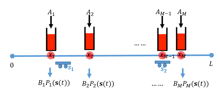
subject to the agent dynamics (1), uncertainty dynamics (5), control constraint |uj(t)|1subscript𝑢𝑗𝑡1|u_{j}(t)|\leq 1, t[0,T]𝑡0𝑇t\in[0,T], and state constraints (2). Figure 1 is a polling model version for problem P1 where each target is associated with a “virtual queue” where uncertainty accumulates with inflow rate Aisubscript𝐴𝑖A_{i}. The service rate of this queue is time-varying and given by BiPi(𝐬(t))subscript𝐵𝑖subscript𝑃𝑖𝐬𝑡B_{i}P_{i}\left(\mathbf{s}(t)\right), controllable through the agent position at time t𝑡t. This interpretation is convenient for characterizing the stability of such a system over a mission time T𝑇T: For each queue, we may require that 0TAi<0TBiPi(𝐬(t))𝑑tsuperscriptsubscript0𝑇subscript𝐴𝑖superscriptsubscript0𝑇subscript𝐵𝑖subscript𝑃𝑖𝐬𝑡differential-d𝑡\int_{0}^{T}A_{i}<\int_{0}^{T}B_{i}P_{i}(\mathbf{s}(t))dt. Alternatively, we may require that each queue becomes empty at least once over [0,T]0𝑇[0,T]. Note that this analogy readily extends to two or three-dimensional settings.
Refer to caption
Figure 1: A 1D polling model interpretation of problem P1

III Optimal control solution

In this section, we derive properties of the optimal control solution of problem P1 and show that it can be reduced to a parametric optimization problem. This will allow us to utilize an Infinitesimal Perturbation Analysis (IPA) gradient estimation approach [12] to find a complete optimal solution through a gradient-based algorithm. We begin by defining the state vector 𝐱(t)=[R1(t),RM(t),s1(t)sN(t)]𝐱𝑡subscript𝑅1𝑡subscript𝑅𝑀𝑡subscript𝑠1𝑡subscript𝑠𝑁𝑡\mathbf{x}(t)=[R_{1}(t),...R_{M}(t),s_{1}(t)...s_{N}(t)] and associated costate vector λ=[λ1(t),,λM(t),λs1(t),,λsN(t)]𝜆subscript𝜆1𝑡subscript𝜆𝑀𝑡subscript𝜆subscript𝑠1𝑡subscript𝜆subscript𝑠𝑁𝑡\lambda=[\lambda_{1}(t),...,\lambda_{M}(t),\lambda_{s_{1}}(t),...,\lambda_{s_{N}}(t)]. As in [3], since the discontinuity in the dynamics of Ri(t)subscript𝑅𝑖𝑡R_{i}(t) in (5), the optimal state trajectory may contain a boundary arc when Ri(t)=0subscript𝑅𝑖𝑡0R_{i}(t)=0 for some i𝑖i; otherwise, the state evolves in an interior arc. Thus, we first analyze such an interior arc. Using (1) and (5), the Hamiltonian is

H(𝐱,λ,𝐮)=i=1MRi(t)+i=1Mλi(t)R˙i(t)+j=1Nλsj(t)uj(t)𝐻𝐱𝜆𝐮superscriptsubscript𝑖1𝑀subscript𝑅𝑖𝑡superscriptsubscript𝑖1𝑀subscript𝜆𝑖𝑡subscript˙𝑅𝑖𝑡superscriptsubscript𝑗1𝑁subscript𝜆subscript𝑠𝑗𝑡subscript𝑢𝑗𝑡H(\mathbf{x},\lambda,\mathbf{u})=\sum_{i=1}^{M}R_{i}(t)+\sum_{i=1}^{M}\lambda_{i}(t)\dot{R}_{i}(t)+\sum_{j=1}^{N}\lambda_{s_{j}}(t)u_{j}(t) (7)

The costate dynamics are

λi˙(t)=HRi(t)=1,λi(T)=0formulae-sequence˙subscript𝜆𝑖𝑡𝐻subscript𝑅𝑖𝑡1subscript𝜆𝑖𝑇0\dot{\lambda_{i}}(t)=-\frac{\partial H}{\partial R_{i}(t)}=-1,\quad\lambda_{i}(T)=0 (8)
λ˙sj(t)=Hsj(t)=i=1Mλi(t)BiPi(𝐬(t))sj(t),λsj(T)=0formulae-sequencesubscript˙𝜆subscript𝑠𝑗𝑡𝐻subscript𝑠𝑗𝑡superscriptsubscript𝑖1𝑀subscript𝜆𝑖𝑡subscript𝐵𝑖subscript𝑃𝑖𝐬𝑡subscript𝑠𝑗𝑡subscript𝜆subscript𝑠𝑗𝑇0\dot{\lambda}_{s_{j}}\left(t\right)=-\frac{\partial H}{\partial s_{j}\left(t\right)}=\sum_{i=1}^{M}\lambda_{i}\left(t\right)B_{i}\frac{\partial P_{i}(\mathbf{s}(t))}{\partial s_{j}(t)},\quad\lambda_{s_{j}}(T)=0 (9)

Applying the Pontryagin Minimum Principle to (7) with 𝐮(t)superscript𝐮𝑡\mathbf{u}^{\star}(t), t[0,T)𝑡0𝑇t\in[0,T), denoting an optimal control, a necessary condition for optimality is

H(𝐱,λ,𝐮)=minuj[1,1], j=1,,NH(𝐱,λ,𝐮)𝐻superscript𝐱superscript𝜆superscript𝐮subscriptformulae-sequencesubscript𝑢𝑗11 𝑗1𝑁𝐻𝐱𝜆𝐮H\left(\mathbf{x}^{\star},\mathbf{\lambda}^{\star},\mathbf{u}^{\star}\right)=\min_{u_{j}\in[-1,1],\text{ }j=1,\ldots,N}H\left(\mathbf{x},\mathbf{\lambda},\mathbf{u}\right) (10)

from which it immediately follows that

uj(t)={1if λsj(t)<01if λsj(t)>0superscriptsubscript𝑢𝑗𝑡cases1if subscript𝜆subscript𝑠𝑗𝑡01if subscript𝜆subscript𝑠𝑗𝑡0u_{j}^{\ast}(t)=\begin{cases}1&\quad\text{if }\lambda_{s_{j}}(t)<0\\ -1&\quad\text{if }\lambda_{s_{j}}(t)>0\end{cases} (11)

Note that there exists a possibility that λsj(t)=0subscript𝜆subscript𝑠𝑗𝑡0\lambda_{s_{j}}\left(t\right)=0 over some finite singular intervals [18], in which case uj(t)superscriptsubscript𝑢𝑗𝑡u_{j}^{\ast}(t) may take values in {{\{ 1,0,1}-1,0,1\}.

Similar to the case of the persistent monitoring problem studied in [3], the complete solution requires solving the costate equations (9), which in turn involves the determination of all points where Ri(t)=0subscript𝑅𝑖𝑡0R_{i}(t)=0, i=1,,M𝑖1𝑀i=1,\ldots,M. This generally involves the solution of a two-point-boundary-value problem. However, we will next prove some structural properties of an optimal trajectory, based on which we show that it is fully characterized by a set of parameters, thus reducing the optimal control problem to a much simpler parametric optimization problem.

We begin by assuming that targets are ordered according to their location so that x1<<xMsubscript𝑥1subscript𝑥𝑀x_{1}<\cdots<x_{M}. Let r=maxj=1,,N{rj}𝑟subscript𝑗1𝑁subscript𝑟𝑗r=\max_{j=1,\ldots,N}\{r_{j}\} and a=max{0,x1r}𝑎0subscript𝑥1𝑟a=\max\{0,x_{1}-r\}, b=min{L,xM+r}𝑏𝐿subscript𝑥𝑀𝑟b=\min\{L,x_{M}+r\}. Thus, if sj(t)<x1rsubscript𝑠𝑗𝑡subscript𝑥1𝑟s_{j}(t)<x_{1}-r or sj(t)>xM+rsubscript𝑠𝑗𝑡subscript𝑥𝑀𝑟s_{j}(t)>x_{M}+r, then it follows from (3) that pij(sj(t))=0subscript𝑝𝑖𝑗subscript𝑠𝑗𝑡0p_{ij}(s_{j}(t))=0 for all targets i=1,,M𝑖1𝑀i=1,\ldots,M. Clearly, this implies that the effective mission space is [a,b]𝑎𝑏[a,b], i.e.,

asj(t)b, j=1,,Nformulae-sequence𝑎subscript𝑠𝑗𝑡𝑏 𝑗1𝑁a\leq s_{j}(t)\leq b,\text{ \ \ }j=1,\ldots,N (12)

imposing an additional state constraint for P1. We will show next that on an optimal trajectory every agent is constrained to move within the interval [x1,xM]subscript𝑥1subscript𝑥𝑀[x_{1},x_{M}]. This implies that every agent must switch its direction no later than reaching the first or last target (possibly after dwelling at the switching point for a finite time interval). To establish this and subsequent results, we will make a technical assumption that no two events altering the dynamics in this system can occur at the exact same time.

Assumption 1: Suppose that an agent switches direction at θ[a,b]𝜃𝑎𝑏\theta\in[a,b]. For any j=1,,N,𝑗1𝑁j=1,\ldots,N, i=1,,M,𝑖1𝑀i=1,\ldots,M, t(0,T)𝑡0𝑇t\in(0,T), and any ϵ>0italic-ϵ0\epsilon>0, if sj(t)=θsubscript𝑠𝑗𝑡𝜃s_{j}(t)=\theta, sj(tϵ)>θsubscript𝑠𝑗𝑡italic-ϵ𝜃s_{j}(t-\epsilon)>\theta or if sj(t)=θsubscript𝑠𝑗𝑡𝜃s_{j}(t)=\theta, sj(tϵ)<θsubscript𝑠𝑗𝑡italic-ϵ𝜃s_{j}(t-\epsilon)<\theta, then either Ri(τ)>0subscript𝑅𝑖𝜏0R_{i}(\tau)>0 for all τ[tϵ,t]𝜏𝑡italic-ϵ𝑡\tau\in[t-\epsilon,t] or Ri(τ)=0subscript𝑅𝑖𝜏0R_{i}(\tau)=0 for all τ[tϵ,t]𝜏𝑡italic-ϵ𝑡\tau\in[t-\epsilon,t].

Proposition 1: In an optimal trajectory, x1sj(t)xMsubscript𝑥1superscriptsubscript𝑠𝑗𝑡subscript𝑥𝑀x_{1}\leq s_{j}^{\ast}(t)\leq x_{M}, t[0,T]𝑡0𝑇t\in[0,T], j=1,,N𝑗1𝑁j=1,\ldots,N.

Proof. We first prove that sj(t)x1superscriptsubscript𝑠𝑗𝑡subscript𝑥1s_{j}^{\ast}(t)\geq x_{1} for any agent j𝑗j. Suppose that sj(t0)=x1superscriptsubscript𝑠𝑗subscript𝑡0subscript𝑥1s_{j}^{\ast}(t_{0})=x_{1} and uj(t0)=1superscriptsubscript𝑢𝑗subscript𝑡01u_{j}^{\ast}(t_{0})=-1. In view of (12), assume that agent j𝑗j reaches a point θ[a,x1)𝜃𝑎subscript𝑥1\theta\in[a,x_{1}) at time t1>t0subscript𝑡1subscript𝑡0t_{1}>t_{0} where it switches direction; we will show that θ[a,x1)𝜃𝑎subscript𝑥1\theta\notin[a,x_{1}) using a contradiction argument. There are two cases to consider:

Case 1: θ=a𝜃𝑎\theta=a. Assuming sj(t1)=asuperscriptsubscript𝑠𝑗subscript𝑡1𝑎s_{j}^{\ast}(t_{1})=a, we first show that λsj(t1)=0superscriptsubscript𝜆subscript𝑠𝑗superscriptsubscript𝑡10\lambda_{s_{j}}^{\ast}(t_{1}^{-})=0 by a contradiction argument. If λsj(t1)0superscriptsubscript𝜆subscript𝑠𝑗superscriptsubscript𝑡10\lambda_{s_{j}}^{\ast}(t_{1}^{-})\neq 0, recall that uj(t1)=1superscriptsubscript𝑢𝑗superscriptsubscript𝑡11u_{j}^{\ast}(t_{1}^{-})=-1, therefore λsj(t1)>0superscriptsubscript𝜆subscript𝑠𝑗superscriptsubscript𝑡10\lambda_{s_{j}}^{\ast}(t_{1}^{-})>0 from (11). Since the constraint asj(t)0𝑎subscript𝑠𝑗𝑡0a-s_{j}(t)\leq 0 is active, λsj(t)superscriptsubscript𝜆subscript𝑠𝑗𝑡\lambda_{s_{j}}^{\ast}(t) may experience a discontinuity so that

λsj(t1)=λsj(t1+)πjsuperscriptsubscript𝜆subscript𝑠𝑗superscriptsubscript𝑡1superscriptsubscript𝜆subscript𝑠𝑗superscriptsubscript𝑡1subscript𝜋𝑗\lambda_{s_{j}}^{\ast}(t_{1}^{-})=\lambda_{s_{j}}^{\ast}(t_{1}^{+})-\pi_{j} (13)

where πj0subscript𝜋𝑗0\pi_{j}\geq 0 is a scalar multiplier associated with the constraint asj(t)0𝑎subscript𝑠𝑗𝑡0a-s_{j}(t)\leq 0. It follows that λsj(t1+)=λsj(t1)+πj>0superscriptsubscript𝜆subscript𝑠𝑗superscriptsubscript𝑡1superscriptsubscript𝜆subscript𝑠𝑗superscriptsubscript𝑡1subscript𝜋𝑗0\lambda_{s_{j}}^{\ast}(t_{1}^{+})=\lambda_{s_{j}}^{\ast}(t_{1}^{-})+\pi_{j}>0. Since the Hamiltonian in (7) and the constraint asj(t)0𝑎subscript𝑠𝑗𝑡0a-s_{j}(t)\leq 0 are not explicit functions of time, we have [18] H(𝐱(t1),λ(t1),𝐮(t1))=H(𝐱(t1+),λ(t1+),𝐮(t1+))superscript𝐻𝐱superscriptsubscript𝑡1𝜆superscriptsubscript𝑡1𝐮superscriptsubscript𝑡1superscript𝐻𝐱superscriptsubscript𝑡1𝜆superscriptsubscript𝑡1𝐮superscriptsubscript𝑡1H^{\ast}(\mathbf{x}(t_{1}^{-}),\mathbf{\lambda}(t_{1}^{-}),\mathbf{u}(t_{1}^{-}))=H^{\ast}(\mathbf{x}(t_{1}^{+}),\lambda(t_{1}^{+}),\mathbf{u}(t_{1}^{+})) which, under Assumption 1, reduces to

λsj(t1)uj(t1)=λsj(t1+)uj(t1+)superscriptsubscript𝜆subscript𝑠𝑗superscriptsubscript𝑡1superscriptsubscript𝑢𝑗superscriptsubscript𝑡1superscriptsubscript𝜆subscript𝑠𝑗superscriptsubscript𝑡1superscriptsubscript𝑢𝑗superscriptsubscript𝑡1\lambda_{s_{j}}^{\ast}(t_{1}^{-})u_{j}^{\ast}(t_{1}^{-})=\lambda_{s_{j}}^{\ast}(t_{1}^{+})u_{j}^{\ast}(t_{1}^{+}) (14)

Recall that λsj(t1)uj(t1)<0superscriptsubscript𝜆subscript𝑠𝑗superscriptsubscript𝑡1superscriptsubscript𝑢𝑗superscriptsubscript𝑡10\lambda_{s_{j}}^{\ast}(t_{1}^{-})u_{j}^{\ast}(t_{1}^{-})<0. However, uj(t1+)0superscriptsubscript𝑢𝑗superscriptsubscript𝑡10u_{j}^{\ast}(t_{1}^{+})\geq 0 (since the agent switches control), therefore λsj(t1+)uj(t1+)0superscriptsubscript𝜆subscript𝑠𝑗superscriptsubscript𝑡1superscriptsubscript𝑢𝑗superscriptsubscript𝑡10\lambda_{s_{j}}^{\ast}(t_{1}^{+})u_{j}^{\ast}(t_{1}^{+})\geq 0 which violates (14). This contradiction implies that λsj(t1)=0superscriptsubscript𝜆subscript𝑠𝑗superscriptsubscript𝑡10\lambda_{s_{j}}^{\ast}(t_{1}^{-})=0. Recalling (4) and (9), we get λ˙sj(t1)=i=1,Ri0Mλi(t1)Birjdj[1pid(sd(t1))]superscriptsubscript˙𝜆subscript𝑠𝑗superscriptsubscript𝑡1superscriptsubscriptformulae-sequence𝑖1subscript𝑅𝑖0𝑀superscriptsubscript𝜆𝑖superscriptsubscript𝑡1subscript𝐵𝑖subscript𝑟𝑗subscriptproduct𝑑𝑗delimited-[]1subscript𝑝𝑖𝑑superscriptsubscript𝑠𝑑superscriptsubscript𝑡1\dot{\lambda}_{s_{j}}^{\ast}(t_{1}^{-})=\sum_{i=1,R_{i}\neq 0}^{M}\lambda_{i}^{\ast}(t_{1}^{-})\frac{B_{i}}{r_{j}}\prod_{d\neq j}[1-p_{id}(s_{d}^{\ast}(t_{1}^{-}))]. Under Assumption 1, there exists δ>0𝛿0\delta>0 such that during interval (t1δ,t1)subscript𝑡1𝛿subscript𝑡1(t_{1}-\delta,t_{1}), no Ri(t)0subscript𝑅𝑖𝑡0R_{i}(t)\geq 0 becomes active, hence no λi(t)superscriptsubscript𝜆𝑖𝑡\lambda_{i}^{\ast}(t) encounters a jump for i=1,,M𝑖1𝑀i=1,\ldots,M and it follows from (8) that λi(t)>0superscriptsubscript𝜆𝑖𝑡0\lambda_{i}^{\ast}(t)>0. Moreover, pid(sd(t))1subscript𝑝𝑖𝑑superscriptsubscript𝑠𝑑𝑡1p_{id}(s_{d}^{\ast}(t))\neq 1 for at least some dj𝑑𝑗d\neq j since we have assumed that M>N𝑀𝑁M>N. Thus, we have λ˙sj(t)>0,superscriptsubscript˙𝜆subscript𝑠𝑗𝑡0\dot{\lambda}_{s_{j}}^{\ast}(t)>0, for all t(t1δ,t1)𝑡subscript𝑡1𝛿subscript𝑡1t\in(t_{1}-\delta,t_{1}). However, since agent j𝑗j is approaching a𝑎a, there exists some δ<δsuperscript𝛿𝛿\delta^{\prime}<\delta, such that uj(t)=1superscriptsubscript𝑢𝑗𝑡1u_{j}^{\ast}(t)=-1 for all t(t1δ,t1)𝑡subscript𝑡1superscript𝛿subscript𝑡1t\in(t_{1}-\delta^{\prime},t_{1}), and λsj(t)0superscriptsubscript𝜆subscript𝑠𝑗𝑡0\lambda_{s_{j}}^{\ast}(t)\geq 0. Thus for t(t1δ,t1)𝑡subscript𝑡1superscript𝛿subscript𝑡1t\in(t_{1}-\delta^{\prime},t_{1}), we have λsj(t)0superscriptsubscript𝜆subscript𝑠𝑗𝑡0\lambda_{s_{j}}^{\ast}(t)\geq 0 and λ˙sj(t)>0superscriptsubscript˙𝜆subscript𝑠𝑗𝑡0\dot{\lambda}_{s_{j}}^{\ast}(t)>0. This contradicts the established fact that λsj(t1)=0superscriptsubscript𝜆subscript𝑠𝑗superscriptsubscript𝑡10\lambda_{s_{j}}^{\ast}(t_{1}^{-})=0. We conclude that θa𝜃𝑎\theta\neq a.

Case 2: θ(a,x1)𝜃𝑎subscript𝑥1\theta\in(a,x_{1}). Assuming sj(t1)=θsuperscriptsubscript𝑠𝑗subscript𝑡1𝜃s_{j}^{\ast}(t_{1})=\theta, we still have uj(t1)=1superscriptsubscript𝑢𝑗superscriptsubscript𝑡11u_{j}^{\ast}(t_{1}^{-})=-1, uj(t1+)0superscriptsubscript𝑢𝑗superscriptsubscript𝑡10u_{j}^{\ast}(t_{1}^{+})\geq 0. Since the Hamiltonian (7) is not an explicit function of time, we have H(𝐱(t1),λ(t1),𝐮(t1))=H(𝐱(t1+),λ(t1+),𝐮(t1+))superscript𝐻𝐱superscriptsubscript𝑡1𝜆superscriptsubscript𝑡1𝐮superscriptsubscript𝑡1superscript𝐻𝐱superscriptsubscript𝑡1𝜆superscriptsubscript𝑡1𝐮superscriptsubscript𝑡1H^{\ast}(\mathbf{x}(t_{1}^{-}),\mathbf{\lambda}(t_{1}^{-}),\mathbf{u}(t_{1}^{-}))=H^{\ast}(\mathbf{x}(t_{1}^{+}),\lambda(t_{1}^{+}),\mathbf{u}(t_{1}^{+})) which leads to (14) under Assumption 1. First, we assume λsj(t1)0superscriptsubscript𝜆subscript𝑠𝑗superscriptsubscript𝑡10\lambda_{s_{j}}^{\ast}(t_{1}^{-})\neq 0. Since uj(t1)<0superscriptsubscript𝑢𝑗superscriptsubscript𝑡10u_{j}^{\ast}(t_{1}^{-})<0, we have λsj(t1)>0superscriptsubscript𝜆subscript𝑠𝑗superscriptsubscript𝑡10\lambda_{s_{j}}^{\ast}(t_{1}^{-})>0 and the left hand side of (14) gives λsj(t1)uj(t1)<0superscriptsubscript𝜆subscript𝑠𝑗superscriptsubscript𝑡1superscriptsubscript𝑢𝑗superscriptsubscript𝑡10\lambda_{s_{j}}^{\ast}(t_{1}^{-})u_{j}^{\ast}(t_{1}^{-})<0. On the other hand, in order to satisfy (14), we must have uj(t1+)>0superscriptsubscript𝑢𝑗superscriptsubscript𝑡10u_{j}^{\ast}(t_{1}^{+})>0 and λsj(t1+)<0superscriptsubscript𝜆subscript𝑠𝑗superscriptsubscript𝑡10\lambda_{s_{j}}^{\ast}(t_{1}^{+})<0. However, if λsj(t1)>0superscriptsubscript𝜆subscript𝑠𝑗superscriptsubscript𝑡10\lambda_{s_{j}}^{\ast}(t_{1}^{-})>0 and λsj(t1+)<0superscriptsubscript𝜆subscript𝑠𝑗superscriptsubscript𝑡10\lambda_{s_{j}}^{\ast}(t_{1}^{+})<0, then either λ˙sj(t1)<0superscriptsubscript˙𝜆subscript𝑠𝑗subscript𝑡10\dot{\lambda}_{s_{j}}^{\ast}(t_{1})<0 and λsj(t1)=0superscriptsubscript𝜆subscript𝑠𝑗subscript𝑡10\lambda_{s_{j}}^{\ast}(t_{1})=0, or λsj(t)superscriptsubscript𝜆subscript𝑠𝑗𝑡\lambda_{s_{j}}^{\ast}(t) experiences a discontinuity at t1subscript𝑡1t_{1}. We show that neither condition is feasible. The first one violates our assumption that λsj(t1)0superscriptsubscript𝜆subscript𝑠𝑗subscript𝑡10\lambda_{s_{j}}^{\ast}(t_{1})\neq 0, while the second one is not feasible since at t=t1𝑡subscript𝑡1t=t_{1} the constraint asj(t)0𝑎subscript𝑠𝑗𝑡0a-s_{j}(t)\leq 0 is not active. This implies that λsj(t1)=0superscriptsubscript𝜆subscript𝑠𝑗superscriptsubscript𝑡10\lambda_{s_{j}}^{\ast}(t_{1}^{-})=0. Again, under Assumption 1, the same argument as in Case 1 can be used to show that λsj(t)0superscriptsubscript𝜆subscript𝑠𝑗𝑡0\lambda_{s_{j}}^{\ast}(t)\geq 0 and λ˙sj(t)>0superscriptsubscript˙𝜆subscript𝑠𝑗𝑡0\dot{\lambda}_{s_{j}}^{\ast}(t)>0 for all t(t1δ,t1)𝑡subscript𝑡1superscript𝛿subscript𝑡1t\in(t_{1}-\delta^{\prime},t_{1}). This contradicts the established fact that λsj(t1)=0superscriptsubscript𝜆subscript𝑠𝑗superscriptsubscript𝑡10\lambda_{s_{j}}^{\ast}(t_{1}^{-})=0 and we conclude that θ(a,x1)𝜃𝑎subscript𝑥1\theta\notin(a,x_{1}).

Combining both cases, we conclude that θ[0,x1)𝜃0subscript𝑥1\theta\notin[0,x_{1}), which implies that sj(t)x1superscriptsubscript𝑠𝑗𝑡subscript𝑥1s_{j}^{\ast}(t)\geq x_{1}. The same line of argument can be used to show that sj(t)xMsuperscriptsubscript𝑠𝑗𝑡subscript𝑥𝑀s_{j}^{\ast}(t)\leq x_{M}.\blacksquare

Proposition 1, in conjunction with (11), leads to the conclusion that the optimal control consists of each agent moving with maximal speed in one direction until it reaches a point in the interval [x1,xM]subscript𝑥1subscript𝑥𝑀[x_{1},x_{M}] where it switches direction. However, the exclusion of the case λsj(t)=0subscript𝜆subscript𝑠𝑗𝑡0\lambda_{s_{j}}(t)=0 allows the possibility of singular arcs along the optimal trajectory, defined as intervals [t1,t2]subscript𝑡1subscript𝑡2[t_{1},t_{2}] such that λsj(t)=0subscript𝜆subscript𝑠𝑗𝑡0\lambda_{s_{j}}(t)=0 for all t[t1,t2]𝑡subscript𝑡1subscript𝑡2t\in[t_{1},t_{2}] and λsj(t1)0subscript𝜆subscript𝑠𝑗superscriptsubscript𝑡10\lambda_{s_{j}}(t_{1}^{-})\neq 0, λsj(t2+)0subscript𝜆subscript𝑠𝑗superscriptsubscript𝑡20\lambda_{s_{j}}(t_{2}^{+})\neq 0. The next result establishes the fact that we can exclude singular arcs from an agent’s trajectory while this agent has no target in its sensing range.

Lemma 1: If |sj(t)xi|>rjsubscript𝑠𝑗𝑡subscript𝑥𝑖subscript𝑟𝑗|s_{j}(t)-x_{i}|>r_{j} for any i=1,,M𝑖1𝑀i=1,\ldots,M, then uj(t)0superscriptsubscript𝑢𝑗𝑡0u_{j}^{\ast}(t)\neq 0.

Proof. We proceed with a contradiction argument. Suppose that uj(t)=0superscriptsubscript𝑢𝑗𝑡0u_{j}^{\ast}(t)=0 for t[t1,t2]𝑡subscript𝑡1subscript𝑡2t\in[t_{1},t_{2}] such that |sj(t1)xi|>rjsuperscriptsubscript𝑠𝑗subscript𝑡1subscript𝑥𝑖subscript𝑟𝑗|s_{j}^{\ast}(t_{1})-x_{i}|>r_{j} for all i=1,,M𝑖1𝑀i=1,\ldots,M and that uj(t)0superscriptsubscript𝑢𝑗𝑡0u_{j}^{\ast}(t)\neq 0 (without loss of generality, let uj(t)=1superscriptsubscript𝑢𝑗𝑡1u_{j}^{\ast}(t)=1) for t>t2𝑡subscript𝑡2t>t_{2} so that |sj(t3)xi|=rjsuperscriptsubscript𝑠𝑗subscript𝑡3subscript𝑥𝑖subscript𝑟𝑗|s_{j}^{\ast}(t_{3})-x_{i}|=r_{j} for some i=1,,M𝑖1𝑀i=1,\ldots,M and |sj(t3+Δ)xi|<rjsuperscriptsubscript𝑠𝑗subscript𝑡3Δsubscript𝑥𝑖subscript𝑟𝑗|s_{j}^{\ast}(t_{3}+\Delta)-x_{i}|<r_{j} for t3+Δ>t3>t2subscript𝑡3Δsubscript𝑡3subscript𝑡2t_{3}+\Delta>t_{3}>t_{2}. In other words, agent j𝑗j eventually reaches a target i𝑖i that it can sense at t=t3𝑡subscript𝑡3t=t_{3}. Assume that uj(t)superscriptsubscript𝑢𝑗𝑡u_{j}^{\ast}(t), t[t1,t3+Δ]𝑡subscript𝑡1subscript𝑡3Δt\in[t_{1},t_{3}+\Delta] is replaced by uj(t)superscriptsubscript𝑢𝑗𝑡u_{j}^{\prime}(t) as follows: uj(t)=1superscriptsubscript𝑢𝑗𝑡1u_{j}^{\prime}(t)=1 for t[t1,t3+Δ+t1t2]𝑡subscript𝑡1subscript𝑡3Δsubscript𝑡1subscript𝑡2t\in[t_{1},t_{3}+\Delta+t_{1}-t_{2}] and uj(t)=0superscriptsubscript𝑢𝑗𝑡0u_{j}^{\prime}(t)=0 for t(t3+Δ+t1t2,t3+Δ]𝑡subscript𝑡3Δsubscript𝑡1subscript𝑡2subscript𝑡3Δt\in(t_{3}+\Delta+t_{1}-t_{2},t_{3}+\Delta]. In other words, the agent moves to reach sj(t3+Δ+t1t2)=sj(t3+Δ)superscriptsubscript𝑠𝑗subscript𝑡3Δsubscript𝑡1subscript𝑡2superscriptsubscript𝑠𝑗subscript𝑡3Δs_{j}^{\prime}(t_{3}+\Delta+t_{1}-t_{2})=s_{j}^{\ast}(t_{3}+\Delta) and then stops. The two controls are thereafter identical. Then, referring to (6) we have t3+Δ+t1t2t3+ΔRi(t)𝑑tt3+Δ+t1t2t3+ΔRi(t)𝑑tsuperscriptsubscriptsubscript𝑡3Δsubscript𝑡1subscript𝑡2subscript𝑡3Δsuperscriptsubscript𝑅𝑖𝑡differential-d𝑡superscriptsubscriptsubscript𝑡3Δsubscript𝑡1subscript𝑡2subscript𝑡3Δsuperscriptsubscript𝑅𝑖𝑡differential-d𝑡\int_{t_{3}+\Delta+t_{1}-t_{2}}^{t_{3}+\Delta}R_{i}^{\prime}(t)dt\leq\int_{t_{3}+\Delta+t_{1}-t_{2}}^{t_{3}+\Delta}R_{i}^{\ast}(t)dt since under uj(t)superscriptsubscript𝑢𝑗𝑡u_{j}^{\prime}(t) the agent may decrease Ri(t)subscript𝑅𝑖𝑡R_{i}(t) over [t3+Δ+t1t2,t3]subscript𝑡3Δsubscript𝑡1subscript𝑡2subscript𝑡3[t_{3}+\Delta+t_{1}-t_{2},t_{3}] whereas under uj(t)superscriptsubscript𝑢𝑗𝑡u_{j}^{\ast}(t) this is impossible since |sj(t)xi|>rjsuperscriptsubscript𝑠𝑗𝑡subscript𝑥𝑖subscript𝑟𝑗|s_{j}^{\ast}(t)-x_{i}|>r_{j} over this time interval. Since the cost in (6) is the same over [0,t3+Δ+t1t2)0subscript𝑡3Δsubscript𝑡1subscript𝑡2[0,t_{3}+\Delta+t_{1}-t_{2}) and (t3+Δ,T],subscript𝑡3Δ𝑇(t_{3}+\Delta,T], it follows that uj(t)=0superscriptsubscript𝑢𝑗𝑡0u_{j}^{\ast}(t)=0 when |sj(t)xi|>rjsubscript𝑠𝑗𝑡subscript𝑥𝑖subscript𝑟𝑗|s_{j}(t)-x_{i}|>r_{j} cannot be optimal unless uj(t)=0superscriptsubscript𝑢𝑗𝑡0u_{j}^{\ast}(t)=0 for all t[0,T]𝑡0𝑇t\in[0,T], i.e., the agent never moves and never senses any target, in which case the cost under uj(t)superscriptsubscript𝑢𝑗𝑡u_{j}^{{}^{\prime}}(t) is still no higher than that under uj(t)superscriptsubscript𝑢𝑗𝑡u_{j}^{\ast}(t).\blacksquare

Based on Lemma 1, we conclude that singular arcs in an agent’s trajectory may occur only while it is sensing a target. Intuitively, this indicates that it may be optimal for an agent to stop moving and dwell in the vicinity of one or more targets that it can sense so as to decrease the associated uncertainty functions to an adequate level before it proceeds along the mission space. The next lemma establishes the fact that if the agent is visiting an isolated target and experiences a singular arc, then the corresponding optimal control is uj(t)=0superscriptsubscript𝑢𝑗𝑡0u_{j}^{\ast}(t)=0. An isolated target with position xisubscript𝑥𝑖x_{i} is defined to be one that satisfies |xixj|>2r,subscript𝑥𝑖subscript𝑥𝑗2𝑟|x_{i}-x_{j}|>2r,for all ji𝑗𝑖j\neq i where r𝑟r was defined earlier as r=maxj=1,,N{rj}𝑟subscript𝑗1𝑁subscript𝑟𝑗r=\max_{j=1,\ldots,N}\{r_{j}\}. Accordingly, the subset I{1,,M}square-image-of-or-equals𝐼1𝑀I\sqsubseteq\{1,\ldots,M\} of isolated targets is defined as

I={i:|xixj|>2r,ji{1,. . .,M},r=maxj=1,. . .,N{rj}}𝐼conditional-set𝑖formulae-sequenceformulae-sequencesubscript𝑥𝑖subscript𝑥𝑗2𝑟𝑗𝑖1. . .𝑀𝑟subscript𝑗1. . .𝑁subscript𝑟𝑗I=\{i:|x_{i}-x_{j}|>2r,j\neq i\in\{1,\makebox[10.00002pt][c]{.\hfil.\hfil.},M\},r=\max_{j=1,\makebox[7.00002pt][c]{.\hfil.\hfil.},N}\{r_{j}\}\} (15)

Lemma 2: Let |sj(t)xk|<rjsuperscriptsubscript𝑠𝑗𝑡subscript𝑥𝑘subscript𝑟𝑗|s_{j}^{\ast}(t)-x_{k}|<r_{j} for some j=1,,N𝑗1𝑁j=1,\ldots,N and isolated target kI𝑘𝐼k\in I. If λsj(t)=0superscriptsubscript𝜆subscript𝑠𝑗𝑡0\lambda_{s_{j}}^{\ast}(t)=0, t[t1,t2]𝑡subscript𝑡1subscript𝑡2t\in[t_{1},t_{2}], then uj(t)=0superscriptsubscript𝑢𝑗𝑡0u_{j}^{\ast}(t)=0.

Proof. The proof is along the same line as Proposition III.3 in [3]. Assume that λsj(t)=0superscriptsubscript𝜆subscript𝑠𝑗𝑡0\lambda_{s_{j}}^{\ast}(t)=0 over a singular arc [t1,t2]subscript𝑡1subscript𝑡2[t_{1},t_{2}]. Let Hsuperscript𝐻absentH^{\ast}\equiv H(𝐱,λ,𝐮)𝐻superscript𝐱superscript𝜆superscript𝐮H(\mathbf{x}^{\ast}\mathbf{,\lambda}^{\ast}\mathbf{,u}^{\ast}). Since the Hamiltonian along an optimal trajectory is a constant, we have dHdt=0𝑑superscript𝐻𝑑𝑡0\frac{dH^{\ast}}{dt}=0. Therefore, recalling (7),

dHdt=i=1M[R˙i(t)+λ˙i(t)R˙i(t)+λi(t)R¨i(t)]𝑑superscript𝐻𝑑𝑡superscriptsubscript𝑖1𝑀delimited-[]superscriptsubscript˙𝑅𝑖𝑡superscriptsubscript˙𝜆𝑖𝑡superscriptsubscript˙𝑅𝑖𝑡superscriptsubscript𝜆𝑖𝑡superscriptsubscript¨𝑅𝑖𝑡\displaystyle\frac{dH^{\ast}}{dt}=\sum_{i=1}^{M}\Big{[}\dot{R}_{i}^{\ast}(t)+\dot{\lambda}_{i}^{\ast}(t)\dot{R}_{i}^{\ast}(t)+\lambda_{i}^{\ast}(t)\ddot{R}_{i}^{\ast}(t)\Big{]}
+j=1N[λ˙sj(t)uj(t)+λsj(t)u˙j(t)]=0superscriptsubscript𝑗1𝑁delimited-[]superscriptsubscript˙𝜆subscript𝑠𝑗𝑡superscriptsubscript𝑢𝑗𝑡superscriptsubscript𝜆subscript𝑠𝑗𝑡superscriptsubscript˙𝑢𝑗𝑡0\displaystyle+\sum_{j=1}^{N}\Big{[}\dot{\lambda}_{s_{j}}^{\ast}(t)u_{j}^{\ast}(t)+\lambda_{s_{j}}^{\ast}(t)\dot{u}_{j}^{\ast}(t)\Big{]}=0

and since λi˙(t)=1˙superscriptsubscript𝜆𝑖𝑡1\dot{\lambda_{i}^{\ast}}(t)=-1 from (8), this reduces to

dHdt=i=1Mλi(t)R¨i(t)+j=1N[λ˙sj(t)uj(t)+λsj(t)u˙j(t)]=0𝑑superscript𝐻𝑑𝑡superscriptsubscript𝑖1𝑀superscriptsubscript𝜆𝑖𝑡superscriptsubscript¨𝑅𝑖𝑡superscriptsubscript𝑗1𝑁delimited-[]superscriptsubscript˙𝜆subscript𝑠𝑗𝑡superscriptsubscript𝑢𝑗𝑡superscriptsubscript𝜆subscript𝑠𝑗𝑡superscriptsubscript˙𝑢𝑗𝑡0\frac{dH^{\ast}}{dt}=\sum_{i=1}^{M}\lambda_{i}^{\ast}(t)\ddot{R}_{i}^{\ast}(t)+\sum_{j=1}^{N}\Big{[}\dot{\lambda}_{s_{j}}^{\ast}(t)u_{j}^{\ast}(t)+\lambda_{s_{j}}^{\ast}(t)\dot{u}_{j}^{\ast}(t)\Big{]}=0 (16)

Define S(t)={j|λsj(t)=0,λ˙sj(t)=0}𝑆𝑡conditional-set𝑗formulae-sequencesubscript𝜆subscript𝑠𝑗𝑡0subscript˙𝜆subscript𝑠𝑗𝑡0S(t)=\{j|\lambda_{s_{j}}(t)=0,\dot{\lambda}_{s_{j}}(t)=0\} as the set of agents in singular arcs at t𝑡t and S¯(t)¯𝑆𝑡\bar{S}(t) as the set of all remaining agents. If jS(t)𝑗𝑆𝑡j\in S(t), then λ˙sj(t)uj(t)+λsj(t)u˙j(t)=0superscriptsubscript˙𝜆subscript𝑠𝑗𝑡superscriptsubscript𝑢𝑗𝑡superscriptsubscript𝜆subscript𝑠𝑗𝑡superscriptsubscript˙𝑢𝑗𝑡0\dot{\lambda}_{s_{j}}^{\ast}(t)u_{j}^{\ast}(t)+\lambda_{s_{j}}^{\ast}(t)\dot{u}_{j}^{\ast}(t)=0. If jS¯(t)𝑗¯𝑆𝑡j\in\bar{S}(t), then λsj(t)u˙j(t)=0superscriptsubscript𝜆subscript𝑠𝑗𝑡superscriptsubscript˙𝑢𝑗𝑡0\lambda_{s_{j}}^{\ast}(t)\dot{u}_{j}^{\ast}(t)=0 since uj(t)=±1superscriptsubscript𝑢𝑗𝑡plus-or-minus1u_{j}^{\ast}(t)=\pm 1 and u˙j(t)=0superscriptsubscript˙𝑢𝑗𝑡0\dot{u}_{j}^{\ast}(t)=0. Therefore, we rewrite (16) as

dHdt=i=1Mλi(t)R¨i(t)+jS¯(t)λ˙sj(t)uj(t)=0𝑑superscript𝐻𝑑𝑡superscriptsubscript𝑖1𝑀superscriptsubscript𝜆𝑖𝑡superscriptsubscript¨𝑅𝑖𝑡subscript𝑗¯𝑆𝑡superscriptsubscript˙𝜆subscript𝑠𝑗𝑡superscriptsubscript𝑢𝑗𝑡0\frac{dH^{\ast}}{dt}=\sum_{i=1}^{M}\lambda_{i}^{\ast}(t)\ddot{R}_{i}^{\ast}(t)+\sum_{j\in\bar{S}(t)}\dot{\lambda}_{s_{j}}^{\ast}(t)u_{j}^{\ast}(t)=0 (17)

Recalling (5), when Ri(t)0subscript𝑅𝑖𝑡0R_{i}(t)\neq 0, we have R˙i=AiBi(1n=1N[1pij(sj(t))])subscript˙𝑅𝑖subscript𝐴𝑖subscript𝐵𝑖1superscriptsubscriptproduct𝑛1𝑁delimited-[]1subscript𝑝𝑖𝑗subscript𝑠𝑗𝑡\dot{R}_{i}=A_{i}-B_{i}\Big{(}1-\prod_{n=1}^{N}\Big{[}1-p_{ij}\big{(}s_{j}(t)\big{)}\Big{]}\Big{)}. Therefore,

R¨i(t)=superscriptsubscript¨𝑅𝑖𝑡absent\displaystyle\ddot{R}_{i}^{\ast}(t)= ddtR˙i(t)𝑑𝑑𝑡superscriptsubscript˙𝑅𝑖𝑡\displaystyle\frac{d}{dt}\dot{R}_{i}^{\ast}(t)
=j=1Nuj(t)Bipij(sj(t))sjdj[1pid(sd(t))]absentsuperscriptsubscript𝑗1𝑁superscriptsubscript𝑢𝑗𝑡subscript𝐵𝑖subscript𝑝𝑖𝑗superscriptsubscript𝑠𝑗𝑡superscriptsubscript𝑠𝑗subscriptproduct𝑑𝑗delimited-[]1subscript𝑝𝑖𝑑superscriptsubscript𝑠𝑑𝑡\displaystyle=-\sum_{j=1}^{N}u_{j}^{\ast}(t)B_{i}\frac{\partial p_{ij}(s_{j}^{\ast}(t))}{\partial s_{j}^{\ast}}\prod_{d\neq j}\Big{[}1-p_{id}(s_{d}^{\ast}(t))\Big{]} (18)

Moreover, from (9), we have

λ˙sj(t)=i=1,Ri0Mλi(t)Bipij(sj(t))sjdj[1pid(sd(t))]superscriptsubscript˙𝜆subscript𝑠𝑗𝑡superscriptsubscriptformulae-sequence𝑖1subscript𝑅𝑖0𝑀superscriptsubscript𝜆𝑖𝑡subscript𝐵𝑖subscript𝑝𝑖𝑗superscriptsubscript𝑠𝑗𝑡superscriptsubscript𝑠𝑗subscriptproduct𝑑𝑗delimited-[]1subscript𝑝𝑖𝑑superscriptsubscript𝑠𝑑𝑡\dot{\lambda}_{s_{j}}^{\ast}(t)=\sum_{i=1,R_{i}\neq 0}^{M}\lambda_{i}^{\ast}(t)B_{i}\frac{\partial p_{ij}(s_{j}^{\ast}(t))}{\partial s_{j}^{\ast}}\prod_{d\neq j}\Big{[}1-p_{id}(s_{d}^{\ast}(t))\Big{]} (19)

Combining (17)-(19), we get

dHdt=𝑑superscript𝐻𝑑𝑡absent\displaystyle\frac{dH^{\ast}}{dt}=
i=1Ri0Mj=1Nuj(t)λi(t)Bipij(sj(t))sjdj[1pid(sd(t))]superscriptsubscript𝑖1subscript𝑅𝑖0𝑀superscriptsubscript𝑗1𝑁superscriptsubscript𝑢𝑗𝑡superscriptsubscript𝜆𝑖𝑡subscript𝐵𝑖subscript𝑝𝑖𝑗superscriptsubscript𝑠𝑗𝑡superscriptsubscript𝑠𝑗subscriptproduct𝑑𝑗delimited-[]1subscript𝑝𝑖𝑑superscriptsubscript𝑠𝑑𝑡\displaystyle-{\sum\limits_{\begin{subarray}{c}{i=1}\\ {R_{i}\neq 0}\end{subarray}}^{M}}\sum_{j=1}^{N}u_{j}^{\ast}(t)\lambda_{i}^{\ast}(t)B_{i}\frac{\partial p_{ij}(s_{j}^{\ast}(t))}{\partial s_{j}^{\ast}}\prod_{d\neq j}\Big{[}1-p_{id}(s_{d}^{\ast}(t))\Big{]}
+jS¯(t)i=1Ri0Muj(t)λi(t)Bipij(sj(t))sjdj[1pid(sd(t))]subscript𝑗¯𝑆𝑡superscriptsubscript𝑖1subscript𝑅𝑖0𝑀superscriptsubscript𝑢𝑗𝑡superscriptsubscript𝜆𝑖𝑡subscript𝐵𝑖subscript𝑝𝑖𝑗superscriptsubscript𝑠𝑗𝑡superscriptsubscript𝑠𝑗subscriptproduct𝑑𝑗delimited-[]1subscript𝑝𝑖𝑑superscriptsubscript𝑠𝑑𝑡\displaystyle+\sum_{j\in\bar{S}(t)}{\sum\limits_{\begin{subarray}{c}{i=1}\\ {R_{i}\neq 0}\end{subarray}}^{M}}u_{j}^{\ast}(t)\lambda_{i}^{\ast}(t)B_{i}\frac{\partial p_{ij}(s_{j}^{\ast}(t))}{\partial s_{j}^{\ast}}\prod_{d\neq j}\Big{[}1-p_{id}(s_{d}^{\ast}(t))\Big{]}
=jS(t)i=1Ri0Muj(t)λi(t)Bipij(sj(t))sjdj[1pid(sd(t))]absentsubscript𝑗𝑆𝑡superscriptsubscript𝑖1subscript𝑅𝑖0𝑀superscriptsubscript𝑢𝑗𝑡superscriptsubscript𝜆𝑖𝑡subscript𝐵𝑖subscript𝑝𝑖𝑗superscriptsubscript𝑠𝑗𝑡superscriptsubscript𝑠𝑗subscriptproduct𝑑𝑗delimited-[]1subscript𝑝𝑖𝑑superscriptsubscript𝑠𝑑𝑡\displaystyle=\sum_{j\in S(t)}{\sum\limits_{\begin{subarray}{c}{i=1}\\ {R_{i}\neq 0}\end{subarray}}^{M}}u_{j}^{\ast}(t)\lambda_{i}^{\ast}(t)B_{i}\frac{\partial p_{ij}(s_{j}^{\ast}(t))}{\partial s_{j}^{\ast}}\prod_{d\neq j}\Big{[}1-p_{id}(s_{d}^{\ast}(t))\Big{]}
=0absent0\displaystyle=0 (20)

Since we have assumed that |sj(t)xk|<rjsuperscriptsubscript𝑠𝑗𝑡subscript𝑥𝑘subscript𝑟𝑗|s_{j}^{\ast}(t)-x_{k}|<r_{j} and k𝑘k is an isolated target, it follows that pkj(sj(t))0subscript𝑝𝑘𝑗superscriptsubscript𝑠𝑗𝑡0p_{kj}(s_{j}^{\ast}(t))\neq 0 and pij(sj(t))=0subscript𝑝𝑖𝑗subscript𝑠𝑗𝑡0p_{ij}(s_{j}(t))=0 if ik𝑖𝑘i\neq k. Therefore, pkj(sj(t))sj0subscript𝑝𝑘𝑗superscriptsubscript𝑠𝑗𝑡superscriptsubscript𝑠𝑗0\frac{\partial p_{kj}(s_{j}^{\ast}(t))}{\partial s_{j}^{\ast}}\neq 0 and pij(sj(t))sj=0subscript𝑝𝑖𝑗superscriptsubscript𝑠𝑗𝑡superscriptsubscript𝑠𝑗0\frac{\partial p_{ij}(s_{j}^{\ast}(t))}{\partial s_{j}^{\ast}}=0 for all ik𝑖𝑘i\neq k and (20) reduces to

jS(t)uj(t)λk(t)Bipkj(sj(t))sjdj[1pkd(sd(t))]=0subscript𝑗𝑆𝑡superscriptsubscript𝑢𝑗𝑡superscriptsubscript𝜆𝑘𝑡subscript𝐵𝑖subscript𝑝𝑘𝑗superscriptsubscript𝑠𝑗𝑡superscriptsubscript𝑠𝑗subscriptproduct𝑑𝑗delimited-[]1subscript𝑝𝑘𝑑superscriptsubscript𝑠𝑑𝑡0\sum_{j\in S(t)}u_{j}^{\ast}(t)\lambda_{k}^{\ast}(t)B_{i}\frac{\partial p_{kj}(s_{j}^{\ast}(t))}{\partial s_{j}^{\ast}}\prod_{d\neq j}\Big{[}1-p_{kd}(s_{d}^{\ast}(t))\Big{]}=0 (21)

Observe that, from (8), λi(t)>0subscript𝜆𝑖𝑡0\lambda_{i}(t)>0 when Ri(t)0,t<Tformulae-sequencesubscript𝑅𝑖𝑡0𝑡𝑇R_{i}(t)\neq 0,t<T. In addition Bi>0subscript𝐵𝑖0B_{i}>0 and dj[1pkd(sd(t))]0subscriptproduct𝑑𝑗delimited-[]1subscript𝑝𝑘𝑑superscriptsubscript𝑠𝑑𝑡0\prod_{d\neq j}[1-p_{kd}(s_{d}^{\ast}(t))]\neq 0. Therefore, to satisfy (21) for all t[t1,t2]𝑡subscript𝑡1subscript𝑡2t\in[t_{1},t_{2}], we must have uj(t)=0,superscriptsubscript𝑢𝑗𝑡0u_{j}^{\ast}(t)=0, for all jS(t)𝑗𝑆𝑡j\in S(t).\blacksquare

We can further establish the fact that if an agent j𝑗j experiences a singular arc while sensing an isolated target k𝑘k, then the optimal point to stop is such that sj(t)=xksuperscriptsubscript𝑠𝑗𝑡subscript𝑥𝑘s_{j}^{\ast}(t)=x_{k}.

Proposition 2: Let |sj(t)xk|<rjsuperscriptsubscript𝑠𝑗𝑡subscript𝑥𝑘subscript𝑟𝑗|s_{j}^{\ast}(t)-x_{k}|<r_{j} for some j=1,,N𝑗1𝑁j=1,\ldots,N and isolated target kI𝑘𝐼k\in I. If λsj(t)=0superscriptsubscript𝜆subscript𝑠𝑗𝑡0\lambda_{s_{j}}^{\ast}(t)=0, t[t1,t2]𝑡subscript𝑡1subscript𝑡2t\in[t_{1},t_{2}], and uj(t1)=uj(t2+)superscriptsubscript𝑢𝑗superscriptsubscript𝑡1superscriptsubscript𝑢𝑗superscriptsubscript𝑡2u_{j}^{\ast}(t_{1}^{-})=u_{j}^{\ast}(t_{2}^{+}), then sj(t)=xksuperscriptsubscript𝑠𝑗𝑡subscript𝑥𝑘s_{j}^{\ast}(t)=x_{k}, t[t1,t2]𝑡subscript𝑡1subscript𝑡2t\in[t_{1},t_{2}].

Proof. By Lemma 2, we know that uj(t)=0superscriptsubscript𝑢𝑗𝑡0u_{j}^{\ast}(t)=0, t[t1,t2]𝑡subscript𝑡1subscript𝑡2t\in[t_{1},t_{2}]. We use a contradiction argument similar to the one used in Lemma 1 to show that sj(t)=xksuperscriptsubscript𝑠𝑗𝑡subscript𝑥𝑘s_{j}^{\ast}(t)=x_{k}, t[t1,t2]𝑡subscript𝑡1subscript𝑡2t\in[t_{1},t_{2}]. Suppose that uj(t1)=1superscriptsubscript𝑢𝑗superscriptsubscript𝑡11u_{j}^{\ast}(t_{1}^{-})=1 (without loss of generality) and that sj(t)=xkΔ<xksuperscriptsubscript𝑠𝑗𝑡subscript𝑥𝑘Δsubscript𝑥𝑘s_{j}^{\ast}(t)=x_{k}-\Delta<x_{k}. Note that at the end of the singular arc uj(t2+)=1superscriptsubscript𝑢𝑗superscriptsubscript𝑡21u_{j}^{\ast}(t_{2}^{+})=1 since uj(t1)=uj(t2+)superscriptsubscript𝑢𝑗superscriptsubscript𝑡1superscriptsubscript𝑢𝑗superscriptsubscript𝑡2u_{j}^{\ast}(t_{1}^{-})=u_{j}^{\ast}(t_{2}^{+}). This implies that sj(t2+Δ)=xk.superscriptsubscript𝑠𝑗subscript𝑡2Δsubscript𝑥𝑘s_{j}^{\ast}(t_{2}+\Delta)=x_{k}. Assume that uj(t)superscriptsubscript𝑢𝑗𝑡u_{j}^{\ast}(t), t[t1,t2+Δ]𝑡subscript𝑡1subscript𝑡2Δt\in[t_{1},t_{2}+\Delta] is replaced by uj(t)superscriptsubscript𝑢𝑗𝑡u_{j}^{\prime}(t) as follows: uj(t)=1superscriptsubscript𝑢𝑗𝑡1u_{j}^{\prime}(t)=1 for t[t1,t1+Δ]𝑡subscript𝑡1subscript𝑡1Δt\in[t_{1},t_{1}+\Delta] and uj(t)=0superscriptsubscript𝑢𝑗𝑡0u_{j}^{\prime}(t)=0 for t(t1+Δ,t2+Δ]𝑡subscript𝑡1Δsubscript𝑡2Δt\in(t_{1}+\Delta,t_{2}+\Delta]. In other words, the agent moves to reach sj(t1+Δ)=sj(t2+Δ)=xksuperscriptsubscript𝑠𝑗subscript𝑡1Δsuperscriptsubscript𝑠𝑗subscript𝑡2Δsubscript𝑥𝑘s_{j}^{\prime}(t_{1}+\Delta)=s_{j}^{\ast}(t_{2}+\Delta)=x_{k} and then stops. The two controls are thereafter identical. Then, referring to (6) we have t1t2+ΔRi(t)𝑑t<t1t2+ΔRi(t)𝑑tsuperscriptsubscriptsubscript𝑡1subscript𝑡2Δsuperscriptsubscript𝑅𝑖𝑡differential-d𝑡superscriptsubscriptsubscript𝑡1subscript𝑡2Δsuperscriptsubscript𝑅𝑖𝑡differential-d𝑡\int_{t_{1}}^{t_{2}+\Delta}R_{i}^{\prime}(t)dt<\int_{t_{1}}^{t_{2}+\Delta}R_{i}^{\ast}(t)dt since R˙i(t)<R˙i(t)superscriptsubscript˙𝑅𝑖𝑡superscriptsubscript˙𝑅𝑖𝑡\dot{R}_{i}^{\ast}(t)<\dot{R}_{i}^{\prime}(t) due to (5) and the fact that pkj(sj(t))subscript𝑝𝑘𝑗subscript𝑠𝑗𝑡p_{kj}(s_{j}(t)) is monotonically decreasing in |sj(t)xk|subscript𝑠𝑗𝑡subscript𝑥𝑘|s_{j}(t)-x_{k}|. Since the cost in (6) is the same over [0,t1)0subscript𝑡1[0,t_{1}) and (t2+Δ,T],subscript𝑡2Δ𝑇(t_{2}+\Delta,T], it follows that sj(t)=xkΔsuperscriptsubscript𝑠𝑗𝑡subscript𝑥𝑘Δs_{j}^{\ast}(t)=x_{k}-\Delta cannot be optimal. The same argument holds for any Δ>0Δ0\Delta>0, leading to the conclusion that sj(t)=xksuperscriptsubscript𝑠𝑗𝑡subscript𝑥𝑘s_{j}^{\ast}(t)=x_{k}, t[t1,t2]𝑡subscript𝑡1subscript𝑡2t\in[t_{1},t_{2}]. A similar argument also applies to the case sj(t)=xk+Δ>xksuperscriptsubscript𝑠𝑗𝑡subscript𝑥𝑘Δsubscript𝑥𝑘s_{j}^{\ast}(t)=x_{k}+\Delta>x_{k}.\blacksquare

Finally, we consider the case with the state constraint (2). We can then prove that this constraint is never active on an optimal trajectory, i.e., agents reverse their directions before making contact with any other agent.

Proposition 3: Under the constraint sj(t)sj+1(t)subscript𝑠𝑗𝑡subscript𝑠𝑗1𝑡s_{j}(t)\leq s_{j+1}(t), on an optimal trajectory, sj(t)sj+1(t)subscript𝑠𝑗𝑡subscript𝑠𝑗1𝑡s_{j}(t)\neq s_{j+1}(t) for all t(0,T),𝑡0𝑇t\in(0,T), j=1N𝑗1𝑁j=1...N.

Proof. The proof is almost identical to that of Proposition III.4 in [3] and is, therefore, omitted.\blacksquare

The above analysis, including Propositions 1-3, fully characterize the structure of the optimal control as consisting of intervals in [0,T]0𝑇[0,T] where uj(t){1,0,1}superscriptsubscript𝑢𝑗𝑡101u_{j}^{\ast}(t)\in\{-1,0,1\} depending entirely on the sign of λsj(t)subscript𝜆subscript𝑠𝑗𝑡\lambda_{s_{j}}(t). Based on this analysis, we can parameterize P1 so that the cost in (6) depends on a set of (i)𝑖(i) switching points where an agent switches its control from uj(t)=±1subscript𝑢𝑗𝑡plus-or-minus1u_{j}(t)=\pm 1 to 1minus-or-plus1\mp 1 or possibly 00, and (ii)𝑖𝑖(ii) dwelling times if an agent switches from uj(t)=±1subscript𝑢𝑗𝑡plus-or-minus1u_{j}(t)=\pm 1 to 00. In other words, the optimal trajectory of each agent j𝑗j is totally characterized by two parameter vectors: switching points 𝜽j=[θj1,θj2θjΓ]subscript𝜽𝑗subscript𝜃𝑗1subscript𝜃𝑗2subscript𝜃𝑗Γ\bm{\theta}_{j}=[\theta_{j1},\theta_{j2}...\theta_{j\Gamma}] and dwelling times 𝝎j=[ωj1,ωj2ωjΓ]subscript𝝎𝑗subscript𝜔𝑗1subscript𝜔𝑗2subscript𝜔𝑗superscriptΓ\bm{\omega}_{j}=[\omega_{j1},\omega_{j2}...\omega_{j\Gamma^{\prime}}] where ΓΓ\Gamma and ΓsuperscriptΓ\Gamma^{\prime} are prior parameters depending on the given time horizon. This defines a hybrid system with state dynamics (1), (5). The dynamics remain unchanged in between events that cause them to change, i.e., the points θj1,,θjΓsubscript𝜃𝑗1subscript𝜃𝑗Γ\theta_{j1},\ldots,\theta_{j\Gamma} above and instants when Ri(t)subscript𝑅𝑖𝑡R_{i}(t) switches from >0absent0>0 to 00 or vice versa. Therefore, the overall cost function (6) can be parametrically expressed as J(𝜽,𝝎)𝐽𝜽𝝎J(\bm{\theta},\bm{\omega}) and rewritten as the sum of costs over corresponding interevent intervals over a given time horizon:

J(𝜽,𝝎)=1Tk=0Kτk(𝜽,𝝎)τk+1(𝜽,𝝎)i=1MRi(t)dt𝐽𝜽𝝎1𝑇superscriptsubscript𝑘0𝐾superscriptsubscriptsubscript𝜏𝑘𝜽𝝎subscript𝜏𝑘1𝜽𝝎superscriptsubscript𝑖1𝑀subscript𝑅𝑖𝑡𝑑𝑡J(\bm{\theta},\bm{\omega})=\frac{1}{T}\sum_{k=0}^{K}\int_{\tau_{k}(\bm{\theta},\bm{\omega})}^{\tau_{k+1}(\bm{\theta},\bm{\omega})}\sum_{i=1}^{M}R_{i}(t)dt (22)

where τksubscript𝜏𝑘\tau_{k} is the k𝑘k-th event time. This will allow us to apply IPA to determine a gradient J(𝜽,𝝎)𝐽𝜽𝝎\nabla J(\bm{\theta},\bm{\omega}) with respect to these parameters and apply any standard gradient-based optimization algorithm to obtain a (locally) optimal solution.

IV Infinitesimal Perturbation Analysis

As concluded in the previous section, optimal agent trajectories may be selected from the family {𝒔(𝜽,𝝎,t,𝒔0)}𝒔𝜽𝝎𝑡subscript𝒔0\{{\bm{s}(\bm{\theta}},\bm{\omega},t,{\bm{s}}_{0})\} with parameter vectors 𝜽𝜽\bm{\theta} and 𝝎𝝎\bm{\omega} and a given initial condition 𝒔0subscript𝒔0{\bm{s}}_{0}. Along these trajectories, agents are subject to dynamics (1) and targets are subject to (5). An event (e.g., an agent stopping at some target xisubscript𝑥𝑖x_{i}) occurring at time τk(𝜽,𝝎)subscript𝜏𝑘𝜽𝝎\tau_{k}({\bm{\theta}},\bm{\omega}) triggers a switch in these state dynamics. IPA specifies how changes in 𝜽𝜽\bm{\theta} and 𝝎𝝎\bm{\omega} influence the state 𝒔(𝜽,𝝎,t,𝒔0)𝒔𝜽𝝎𝑡subscript𝒔0{\bm{s}(\bm{\theta}},\bm{\omega},t,{\bm{s}}_{0}), as well as event times τk(𝜽,𝝎)subscript𝜏𝑘𝜽𝝎\tau_{k}({\bm{\theta}},\bm{\omega}), k=1,2,𝑘12k=1,2,\ldots, and, ultimately the cost function (22). We briefly review next the IPA framework for general stochastic hybrid systems as presented in [12].

Let {τk(θ)}subscript𝜏𝑘𝜃\{\tau_{k}(\theta)\}, k=1,,K𝑘1𝐾k=1,\ldots,K, denote the occurrence times of all events in the state trajectory of a hybrid system with dynamics x˙=fk(x,θ,t)˙𝑥subscript𝑓𝑘𝑥𝜃𝑡\dot{x}\ =\ f_{k}(x,\theta,t) over an interval [τk(θ),τk+1(θ))subscript𝜏𝑘𝜃subscript𝜏𝑘1𝜃[\tau_{k}(\theta),\tau_{k+1}(\theta)), where θΘ𝜃Θ\theta\in\Theta is some parameter vector and ΘΘ\Theta is a given compact, convex set. For convenience, we set τ0=0subscript𝜏00\tau_{0}=0 and τK+1=Tsubscript𝜏𝐾1𝑇\tau_{K+1}=T. We use the Jacobian matrix notation: x(t)x(θ,t)θsuperscript𝑥𝑡𝑥𝜃𝑡𝜃x^{\prime}(t)\equiv\frac{\partial x(\theta,t)}{\partial\theta} and τkτk(θ)θsuperscriptsubscript𝜏𝑘subscript𝜏𝑘𝜃𝜃\tau_{k}^{\prime}\equiv\frac{\partial\tau_{k}(\theta)}{\partial\theta}, for all state and event time derivatives. It is shown in [12] that

ddtx(t)=fk(t)xx(t)+fk(t)θ𝑑𝑑𝑡superscript𝑥𝑡subscript𝑓𝑘𝑡𝑥superscript𝑥𝑡subscript𝑓𝑘𝑡𝜃\frac{d}{dt}x^{\prime}(t)=\frac{\partial f_{k}(t)}{\partial x}x^{\prime}(t)+\frac{\partial f_{k}(t)}{\partial\theta} (23)

for t[τk,τk+1)𝑡subscript𝜏𝑘subscript𝜏𝑘1t\in[\tau_{k},\tau_{k+1}) with boundary condition:

x(τk+)=x(τk)+[fk1(τk)fk(τk+)]τksuperscript𝑥superscriptsubscript𝜏𝑘superscript𝑥superscriptsubscript𝜏𝑘delimited-[]subscript𝑓𝑘1superscriptsubscript𝜏𝑘subscript𝑓𝑘superscriptsubscript𝜏𝑘superscriptsubscript𝜏𝑘x^{\prime}(\tau_{k}^{+})=x^{\prime}(\tau_{k}^{-})+[f_{k-1}(\tau_{k}^{-})-f_{k}(\tau_{k}^{+})]\tau_{k}^{\prime} (24)

for k=0,K𝑘0𝐾k=0,...K. In order to complete the evaluation of x(τk+)superscript𝑥superscriptsubscript𝜏𝑘x^{\prime}(\tau_{k}^{+}) in (24), we need to determine τksuperscriptsubscript𝜏𝑘\tau_{k}^{\prime}. If the event at τksubscript𝜏𝑘\tau_{k} is exogenous, τk=0superscriptsubscript𝜏𝑘0\tau_{k}^{\prime}=0. However, if the event is endogenous, there exists a continuously differentiable function gk:n×Θ:subscript𝑔𝑘superscript𝑛Θg_{k}:\mathbb{R}^{n}\times\Theta\rightarrow\mathbb{R} such that τk=min{t>τk1:gk(x(θ,t),θ)=0}subscript𝜏𝑘:𝑡subscript𝜏𝑘1subscript𝑔𝑘𝑥𝜃𝑡𝜃0\tau_{k}\ =\ \min\{t>\tau_{k-1}\ :\ g_{k}\left(x\left(\theta,t\right),\theta\right)=0\} and

τk=[gkxfk(τk)]1(gkθ+gkxx(τk))superscriptsubscript𝜏𝑘superscriptdelimited-[]subscript𝑔𝑘𝑥subscript𝑓𝑘superscriptsubscript𝜏𝑘1subscript𝑔𝑘𝜃subscript𝑔𝑘𝑥superscript𝑥superscriptsubscript𝜏𝑘\tau_{k}^{\prime}=-[\frac{\partial g_{k}}{\partial x}f_{k}(\tau_{k}^{-})]^{-1}(\frac{\partial g_{k}}{\partial\theta}+\frac{\partial g_{k}}{\partial x}x^{\prime}(\tau_{k}^{-})) (25)

as long as gkxfk(τk)0subscript𝑔𝑘𝑥subscript𝑓𝑘superscriptsubscript𝜏𝑘0\frac{\partial g_{k}}{\partial x}f_{k}(\tau_{k}^{-})\neq 0. (details may be found in [12]).

Denote the time-varying cost along a given trajectory as L(x,θ,t)𝐿𝑥𝜃𝑡L(x,\theta,t), so the cost in the k𝑘k-th interevent interval is Jk(x,θ)=τkτk+1L(x,θ,t)𝑑tsubscript𝐽𝑘𝑥𝜃superscriptsubscriptsubscript𝜏𝑘subscript𝜏𝑘1𝐿𝑥𝜃𝑡differential-d𝑡J_{k}(x,\theta)=\int_{\tau_{k}}^{\tau_{k+1}}L(x,\theta,t)dt and the total cost is J(x,θ)=k=0KJk(x,θ)𝐽𝑥𝜃superscriptsubscript𝑘0𝐾subscript𝐽𝑘𝑥𝜃J(x,\theta)=\sum_{k=0}^{K}J_{k}(x,\theta). Differentiating and applying the Leibnitz rule with the observation that all terms of the form L(x(τk),θ,τk)τk𝐿𝑥subscript𝜏𝑘𝜃subscript𝜏𝑘superscriptsubscript𝜏𝑘L(x(\tau_{k}),\theta,\tau_{k})\tau_{k}^{\prime} are mutually canceled with τ0=0,τK+1=Tformulae-sequencesubscript𝜏00subscript𝜏𝐾1𝑇\tau_{0}=0,\tau_{K+1}=T fixed, we obtain

J(x,θ)θ𝐽𝑥𝜃𝜃\displaystyle\frac{\partial J(x,\theta)}{\partial\theta} =k=0Kθτkτk+1L(x,θ,t)𝑑tabsentsuperscriptsubscript𝑘0𝐾𝜃superscriptsubscriptsubscript𝜏𝑘subscript𝜏𝑘1𝐿𝑥𝜃𝑡differential-d𝑡\displaystyle=\sum_{k=0}^{K}\frac{\partial}{\partial\theta}\int_{\tau_{k}}^{\tau_{k+1}}L(x,\theta,t)dt
=k=0Kτkτk+1L(x,θ,t)xx(t)+L(x,θ,t)θdtabsentsuperscriptsubscript𝑘0𝐾superscriptsubscriptsubscript𝜏𝑘subscript𝜏𝑘1𝐿𝑥𝜃𝑡𝑥superscript𝑥𝑡𝐿𝑥𝜃𝑡𝜃𝑑𝑡\displaystyle=\sum_{k=0}^{K}\int_{\tau_{k}}^{\tau_{k+1}}\frac{\partial L(x,\theta,t)}{\partial x}x^{\prime}(t)+\frac{\partial L(x,\theta,t)}{\partial\theta}dt (26)

In our setting, we have L(x,θ,t)=i=1MRi(t)𝐿𝑥𝜃𝑡superscriptsubscript𝑖1𝑀subscript𝑅𝑖𝑡L(x,\theta,t)=\sum_{i=1}^{M}R_{i}(t) from (22), which is not an explicit function of the state 𝐱(t)=[R1(t),RM(t),s1(t)sN(t)]𝐱𝑡subscript𝑅1𝑡subscript𝑅𝑀𝑡subscript𝑠1𝑡subscript𝑠𝑁𝑡\mathbf{x}(t)=[R_{1}(t),...R_{M}(t),s_{1}(t)...s_{N}(t)]. Thus, the gradient J(𝜽,𝝎)=[J(𝜽,𝝎)𝜽,J(𝜽,𝝎)𝝎]T𝐽𝜽𝝎superscript𝐽𝜽𝝎𝜽𝐽𝜽𝝎𝝎T\nabla J(\bm{\theta},\bm{\omega})=[\frac{\partial J(\bm{\theta},\bm{\omega})}{\partial\bm{\theta}},\frac{\partial J(\bm{\theta},\bm{\omega})}{\partial\bm{\omega}}]^{\text{T}} reduces to

J(𝜽,𝝎)=1Tk=0Ki=1Mτk(𝜽,𝝎)τk+1(𝜽,𝝎)Ri(t)𝑑t𝐽𝜽𝝎1𝑇superscriptsubscript𝑘0𝐾superscriptsubscript𝑖1𝑀superscriptsubscriptsubscript𝜏𝑘𝜽𝝎subscript𝜏𝑘1𝜽𝝎subscript𝑅𝑖𝑡differential-d𝑡\nabla J(\bm{\theta},\bm{\omega})=\frac{1}{T}\sum_{k=0}^{K}\sum_{i=1}^{M}\int_{\tau_{k}(\bm{\theta},\bm{\omega})}^{\tau_{k+1}(\bm{\theta},\bm{\omega})}\nabla R_{i}(t)dt (27)

where Ri(t)=[Ri(t)𝜽,Ri(t)𝝎]Tsubscript𝑅𝑖𝑡superscriptsubscript𝑅𝑖𝑡𝜽subscript𝑅𝑖𝑡𝝎T\nabla R_{i}(t)=[\frac{\partial R_{i}(t)}{\partial\bm{\theta}},\frac{\partial R_{i}(t)}{\partial\bm{\omega}}]^{\text{T}}.

Applying (23)(24)(25), we can evaluate Ri(t)subscript𝑅𝑖𝑡\nabla R_{i}(t). In contrast to [3], in our problem agents are allowed to dwell on every target and IPA will optimize these dwelling times. Therefore, we need to consider all possible forms of control sequences: (i)𝑖(i) ±10plus-or-minus10\pm 1\rightarrow 0, (ii)𝑖𝑖(ii) 0±10plus-or-minus10\rightarrow\pm 1, and (iii)𝑖𝑖𝑖(iii) ±11plus-or-minus1minus-or-plus1\pm 1\rightarrow\mp 1. We can then obtain from (5):

Ri(t)θjξ=Ri(τk+)θjξ{0if Ri(t)=0,Ai<BiPi(𝐬(t))Gsj(τk+)θjξ(tτk)otherwisesubscript𝑅𝑖𝑡subscript𝜃𝑗𝜉subscript𝑅𝑖superscriptsubscript𝜏𝑘subscript𝜃𝑗𝜉casesformulae-sequence0if subscript𝑅𝑖𝑡0subscript𝐴𝑖subscript𝐵𝑖subscript𝑃𝑖𝐬𝑡otherwise𝐺subscript𝑠𝑗superscriptsubscript𝜏𝑘subscript𝜃𝑗𝜉𝑡subscript𝜏𝑘otherwiseotherwise\frac{\partial R_{i}(t)}{\partial\theta_{j\xi}}=\frac{\partial R_{i}(\tau_{k}^{+})}{\partial\theta_{j\xi}}-\begin{cases}0\quad\text{if }R_{i}(t)=0,A_{i}<B_{i}P_{i}(\mathbf{s}(t))\\ G\frac{\partial s_{j}(\tau_{k}^{+})}{\partial\theta_{j\xi}}(t-\tau_{k})\quad\text{otherwise}\end{cases} (28)
Ri(t)ωjξ=Ri(τk+)ωjξ{0if Ri(t)=0,Ai<BiPi(𝐬(t))Gsj(τk+)ωjξ(tτk)otherwisesubscript𝑅𝑖𝑡subscript𝜔𝑗𝜉subscript𝑅𝑖superscriptsubscript𝜏𝑘subscript𝜔𝑗𝜉casesformulae-sequence0if subscript𝑅𝑖𝑡0subscript𝐴𝑖subscript𝐵𝑖subscript𝑃𝑖𝐬𝑡otherwise𝐺subscript𝑠𝑗superscriptsubscript𝜏𝑘subscript𝜔𝑗𝜉𝑡subscript𝜏𝑘otherwiseotherwise\frac{\partial R_{i}(t)}{\partial\omega_{j\xi}}=\frac{\partial R_{i}(\tau_{k}^{+})}{\partial\omega_{j\xi}}-\begin{cases}0\quad\text{if }R_{i}(t)=0,A_{i}<B_{i}P_{i}(\mathbf{s}(t))\\ G\frac{\partial s_{j}(\tau_{k}^{+})}{\partial\omega_{j\xi}}(t-\tau_{k})\quad\text{otherwise}\end{cases} (29)

where G=Bidj[1pi(sd(t))]pi(sj)sj𝐺subscript𝐵𝑖subscriptproduct𝑑𝑗delimited-[]1subscript𝑝𝑖subscript𝑠𝑑𝑡subscript𝑝𝑖subscript𝑠𝑗subscript𝑠𝑗G=B_{i}\prod_{d\neq j}\big{[}1-p_{i}(s_{d}(t))\big{]}\frac{\partial p_{i}(s_{j})}{\partial s_{j}} and pi(sj)sj=±1rjsubscript𝑝𝑖subscript𝑠𝑗subscript𝑠𝑗plus-or-minus1subscript𝑟𝑗\frac{\partial p_{i}(s_{j})}{s_{j}}=\pm\frac{1}{r_{j}}.

First, let us consider the events that cause switches in R˙i(t)subscript˙𝑅𝑖𝑡\dot{R}_{i}(t) in (5) at time τksubscript𝜏𝑘\tau_{k}. For these events, the dynamics of sj(t)subscript𝑠𝑗𝑡s_{j}(t) are continuous so that sj(τk)=sj(τk+)subscript𝑠𝑗superscriptsubscript𝜏𝑘subscript𝑠𝑗superscriptsubscript𝜏𝑘\nabla s_{j}(\tau_{k}^{-})=\nabla s_{j}(\tau_{k}^{+}). For target i𝑖i,

Ri(τk+)={Ri(τk)if R˙i(τk)=0,R˙i(τk+)=AiBiPi(𝒔(τk+)).0if R˙i(τk)=AiBiPi(𝒔(τk)),R˙i(τk+)=0.subscript𝑅𝑖superscriptsubscript𝜏𝑘casessubscript𝑅𝑖superscriptsubscript𝜏𝑘if subscript˙𝑅𝑖superscriptsubscript𝜏𝑘0otherwisesubscript˙𝑅𝑖superscriptsubscript𝜏𝑘subscript𝐴𝑖subscript𝐵𝑖subscript𝑃𝑖𝒔superscriptsubscript𝜏𝑘0if subscript˙𝑅𝑖superscriptsubscript𝜏𝑘subscript𝐴𝑖subscript𝐵𝑖subscript𝑃𝑖𝒔superscriptsubscript𝜏𝑘otherwisesubscript˙𝑅𝑖superscriptsubscript𝜏𝑘0\nabla R_{i}(\tau_{k}^{+})=\begin{cases}\nabla R_{i}(\tau_{k}^{-})&\text{{if }}\dot{R}_{i}(\tau_{k}^{-})=0,\\ &\dot{R}_{i}(\tau_{k}^{+})=A_{i}-B_{i}P_{i}({\bm{s}}(\tau_{k}^{+})).\\ 0&\text{{if }}\dot{R}_{i}(\tau_{k}^{-})=A_{i}-B_{i}P_{i}({\bm{s}}(\tau_{k}^{-})),\\ &\dot{R}_{i}(\tau_{k}^{+})=0.\end{cases} (30)

Second, let us consider events that cause switches in s˙j(t)=uj(t)subscript˙𝑠𝑗𝑡subscript𝑢𝑗𝑡\dot{s}_{j}(t)=u_{j}(t) at time τksubscript𝜏𝑘\tau_{k}. For these events, the dynamics of Ri(t)subscript𝑅𝑖𝑡R_{i}(t) are continuous so that Ri(τk)=Ri(τk+)subscript𝑅𝑖superscriptsubscript𝜏𝑘subscript𝑅𝑖superscriptsubscript𝜏𝑘\nabla R_{i}(\tau_{k}^{-})=\nabla R_{i}(\tau_{k}^{+}). In order to evaluate (28) and (29), we need sj(τk+)θjξsubscript𝑠𝑗superscriptsubscript𝜏𝑘subscript𝜃𝑗𝜉\frac{\partial s_{j}(\tau_{k}^{+})}{\partial\theta_{j\xi}} and sj(τk+)ωjξsubscript𝑠𝑗superscriptsubscript𝜏𝑘subscript𝜔𝑗𝜉\frac{\partial s_{j}(\tau_{k}^{+})}{\partial\omega_{j\xi}}. Clearly, these are not affected by future events and we only have to consider the current and prior control switches. Let θjξsubscript𝜃𝑗𝜉\theta_{j\xi} and ωjξsubscript𝜔𝑗𝜉\omega_{j\xi} be the current switching point and dwelling time. Again, applying (23)(24)(25), we have

Case 1: uj(τk)=±1,uj(τk+)=0formulae-sequencesubscript𝑢𝑗superscriptsubscript𝜏𝑘plus-or-minus1subscript𝑢𝑗superscriptsubscript𝜏𝑘0u_{j}(\tau_{k}^{-})=\pm 1,u_{j}(\tau_{k}^{+})=0

sjθjl(τk+)={1if l=ξ0if l<ξsubscript𝑠𝑗subscript𝜃𝑗𝑙superscriptsubscript𝜏𝑘cases1if 𝑙𝜉0if 𝑙𝜉\displaystyle\frac{\partial s_{j}}{\partial\theta_{jl}}(\tau_{k}^{+})=\begin{cases}1&\text{if }l=\xi\\ 0&\text{if }l<\xi\end{cases} (31)
sjωjl(τk+)=0for all lξformulae-sequencesubscript𝑠𝑗subscript𝜔𝑗𝑙superscriptsubscript𝜏𝑘0for all 𝑙𝜉\displaystyle\frac{\partial s_{j}}{\partial\omega_{jl}}(\tau_{k}^{+})=0\quad\text{for all }l\leq\xi (32)

Case 2: uj(τk)=0,uj(τk+)=±1formulae-sequencesubscript𝑢𝑗superscriptsubscript𝜏𝑘0subscript𝑢𝑗superscriptsubscript𝜏𝑘plus-or-minus1u_{j}(\tau_{k}^{-})=0,u_{j}(\tau_{k}^{+})=\pm 1

sjθjl(τk+)={sjθjl(τk)uj(τk+)sgn(θjξθj(ξ1))if l=ξsjθjl(τk)uj(τk+)[sgn(θjlθj(l1))sgn(θj(l+1)θjl)]if l<ξ\frac{\partial s_{j}}{\partial\theta_{jl}}(\tau_{k}^{+})=\begin{cases}\frac{\partial s_{j}}{\partial\theta_{jl}}(\tau_{k}^{-})-u_{j}(\tau_{k}^{+})sgn\big{(}\theta_{j\xi}-\theta_{j(\xi-1)}\big{)}&\text{if }l=\xi\\ \frac{\partial s_{j}}{\partial\theta_{jl}}(\tau_{k}^{-})-u_{j}(\tau_{k}^{+})\Big{[}sgn(\theta_{jl}-\theta_{j(l-1)})&\\ \quad\quad\quad\quad\quad\quad\quad-sgn(\theta_{j(l+1)}-\theta_{jl})\Big{]}&\text{if }l<\xi\\ &\end{cases} (33)
sjωjl(τk+)=uj(τk+)for all lξformulae-sequencesubscript𝑠𝑗subscript𝜔𝑗𝑙superscriptsubscript𝜏𝑘subscript𝑢𝑗superscriptsubscript𝜏𝑘for all 𝑙𝜉\frac{\partial s_{j}}{\partial\omega_{jl}}(\tau_{k}^{+})=-u_{j}(\tau_{k}^{+})\quad\text{for all }l\leq\xi (34)

Case 3: uj(τk)=±1,uj(τk+)=1formulae-sequencesubscript𝑢𝑗superscriptsubscript𝜏𝑘plus-or-minus1subscript𝑢𝑗superscriptsubscript𝜏𝑘minus-or-plus1u_{j}(\tau_{k}^{-})=\pm 1,u_{j}(\tau_{k}^{+})=\mp 1

sjθjl(τk+)={2if l=ξsjθjl(τk)if l<ξsubscript𝑠𝑗subscript𝜃𝑗𝑙superscriptsubscript𝜏𝑘cases2if 𝑙𝜉subscript𝑠𝑗subscript𝜃𝑗𝑙superscriptsubscript𝜏𝑘if 𝑙𝜉\frac{\partial s_{j}}{\partial\theta_{jl}}(\tau_{k}^{+})=\begin{cases}2&\text{if }l=\xi\\ -\frac{\partial s_{j}}{\partial\theta_{jl}}(\tau_{k}^{-})&\text{if }l<\xi\end{cases} (35)

Details of these derivations can be found in [3]. An important difference arises in Case 2 above, where τk=|θj1a|+ωj1++|θjξθj(ξ1)|+ωjξsubscript𝜏𝑘subscript𝜃𝑗1𝑎subscript𝜔𝑗1subscript𝜃𝑗𝜉subscript𝜃𝑗𝜉1subscript𝜔𝑗𝜉\tau_{k}=|\theta_{j1}-a|+\omega_{j1}+...+|\theta_{j\xi}-\theta_{j(\xi-1)}|+\omega_{j\xi}. We eliminate the constraints on the switching location that θjξθj(ξ1)subscript𝜃𝑗𝜉subscript𝜃𝑗𝜉1\theta_{j\xi}\leq\theta_{j(\xi-1)} if ξ𝜉\xi is even and θjξθj(ξ1)subscript𝜃𝑗𝜉subscript𝜃𝑗𝜉1\theta_{j\xi}\geq\theta_{j(\xi-1)} if ξ𝜉\xi is odd.

The event excitation problem. Note that all derivative updates above are limited to events occurring at times τk(𝜽,𝝎)subscript𝜏𝑘𝜽𝝎\tau_{k}({\bm{\theta}},\bm{\omega}), k=1,2,𝑘12k=1,2,\ldots. Thus, this approach is scalable in the number of events characterizing the hybrid system, not its state space. While this is a distinct advantage, it also involves a potential drawback. In particular, it assumes that the events involved in IPA updates are observable along a state trajectory. However, if the current trajectory never reaches the vicinity of any target so as to be able to sense it and affect the overall uncertainty cost function, then any small perturbation to the trajectory will have no effect on the cost. As a result, IPA will fail as illustrated in Fig. 2: here, the single agent trajectory s1(𝜽,𝝎,t)subscript𝑠1𝜽𝝎𝑡s_{1}({\bm{\theta}},\bm{\omega},t) is limited to include no event. Thus, if a gradient-based procedure is initialized with such s1(𝜽,𝝎,t)subscript𝑠1𝜽𝝎𝑡s_{1}({\bm{\theta}},\bm{\omega},t), no event involved in the evaluation of Ri(t)subscript𝑅𝑖𝑡\nabla R_{i}(t) is “excited” and the cost gradient remains zero.

Refer to caption
Figure 2: An example of no event excitation leading to a failure of IPA finding an optimal agent trajectory. The yellow bar is the segment of the space covered by the agent.

In order to overcome this problem, we propose a modification of our cost metric by introducing a function V()𝑉V(\cdot) with the property of “spreading” the value of some Ri(t)subscript𝑅𝑖𝑡R_{i}(t) over all points wΩ[0,L]𝑤Ω0𝐿w\in\Omega\equiv[0,L]. Recalling Proposition 1, we limit ourselves to the subset =[x1,xM]Ωsubscript𝑥1subscript𝑥𝑀Ω\mathcal{B}=[x_{1},x_{M}]\subset\Omega. Then, for all points w𝑤w\in\mathcal{B}, we define V(w,t)𝑉𝑤𝑡V(w,t) as a continuous density function which results in a total value equivalent to the weighted sum of the target values i=1MRi(t)superscriptsubscript𝑖1𝑀subscript𝑅𝑖𝑡\sum_{i=1}^{M}R_{i}(t). We impose the condition that V(w,t)𝑉𝑤𝑡V(w,t) be monotonically decreasing in the Euclidean distance wxinorm𝑤subscript𝑥𝑖\|w-x_{i}\|. More precisely, we define di+(w)=max(wxi,r)superscriptsubscript𝑑𝑖𝑤norm𝑤subscript𝑥𝑖𝑟d_{i}^{+}(w)=\max\big{(}\|w-x_{i}\|,r\big{)} where r=minj=1,,N{rj}𝑟subscript𝑗1𝑁subscript𝑟𝑗r=\min_{j=1,\ldots,N}\{r_{j}\} which ensures that di+(w)rsuperscriptsubscript𝑑𝑖𝑤𝑟d_{i}^{+}(w)\geq r. Thus, di+(w)=r>0superscriptsubscript𝑑𝑖𝑤𝑟0d_{i}^{+}(w)=r>0 is fixed for all points within the target’s vicinity, w[xir,xi+r]𝑤subscript𝑥𝑖𝑟subscript𝑥𝑖𝑟w\in[x_{i}-r,x_{i}+r]. We define

V(w,t)=i=1MαiRi(t)di+(w)𝑉𝑤𝑡superscriptsubscript𝑖1𝑀subscript𝛼𝑖subscript𝑅𝑖𝑡superscriptsubscript𝑑𝑖𝑤V(w,t)=\sum_{i=1}^{M}\frac{\alpha_{i}R_{i}(t)}{d_{i}^{+}(w)} (36)

Note that V(w,t)𝑉𝑤𝑡V(w,t) corresponds to the “total weighted reward density” at w𝑤w\in\mathcal{B}. The weight αisubscript𝛼𝑖\alpha_{i} may be included to capture the relative importance of targets, but we shall henceforth set αi=1subscript𝛼𝑖1\alpha_{i}=1 for all i=1,,M𝑖1𝑀i=1,\ldots,M for simplicity. In order to differentiate points w𝑤w\in\mathcal{B} in terms of their location relative to the agents states sj(t)subscript𝑠𝑗𝑡s_{j}(t), j=1,,N𝑗1𝑁j=1,\ldots,N, we also define the travel cost function

Q(w,𝐬(t))=j=1Nsj(t)w𝑄𝑤𝐬𝑡superscriptsubscript𝑗1𝑁normsubscript𝑠𝑗𝑡𝑤Q(w,\mathbf{s}(t))=\sum_{j=1}^{N}\|s_{j}(t)-w\| (37)

Using these definitions we introduce a new objective function component, which is added to the objective function in (6):

J2(t)=Q(w,𝐬(t))V(w,t)𝑑wsubscript𝐽2𝑡subscript𝑄𝑤𝐬𝑡𝑉𝑤𝑡differential-d𝑤J_{2}(t)=\int_{\mathcal{B}}Q(w,\mathbf{s}(t))V(w,t)dw (38)

The significance of J2(t)subscript𝐽2𝑡J_{2}(t) is that it accounts for the movement of agents through Q(w,𝐬(t))𝑄𝑤𝐬𝑡Q(w,{\mathbf{s}}(t)) and captures the target state values through V(w,t)𝑉𝑤𝑡V(w,t). Introducing this term in the objective function in the following creates a non-zero gradient even if the agent trajectories are not passing through any targets. We now define the metrics in (22) as J1(t)subscript𝐽1𝑡J_{1}(t) and incorporate the parametric J2(t)subscript𝐽2𝑡J_{2}(t) as an addition.

min𝜽Θ,𝝎0J(𝜽,𝝎,T)=1T0T[J1(𝜽,𝝎,t)+eβtJ2(𝜽,𝝎,t)]𝑑tsubscriptformulae-sequence𝜽Θ𝝎0𝐽𝜽𝝎𝑇1𝑇superscriptsubscript0𝑇delimited-[]subscript𝐽1𝜽𝝎𝑡superscript𝑒𝛽𝑡subscript𝐽2𝜽𝝎𝑡differential-d𝑡\min\limits_{\bm{\theta}\in\Theta,\bm{\omega}\geq 0}J(\bm{\theta},\bm{\omega},T)=\frac{1}{T}\int_{0}^{T}\big{[}J_{1}(\bm{\theta},\bm{\omega},t)+e^{-\beta t}J_{2}(\bm{\theta},\bm{\omega},t)\big{]}dt (39)

where J1(𝜽,𝝎,t)=i=1MRi(t)subscript𝐽1𝜽𝝎𝑡superscriptsubscript𝑖1𝑀subscript𝑅𝑖𝑡J_{1}(\bm{\theta},\bm{\omega},t)=\sum_{i=1}^{M}R_{i}(t) is the original uncertainty metric. This creates a continuous potential field for the agents which ensures a non-zero cost gradient even when the trajectories do not excite any events. This non-zero gradient will induce trajectory adjustments that naturally bring them toward ones with observable events. The inclusion of the factor eβtsuperscript𝑒𝛽𝑡e^{-\beta t} with β>0𝛽0\beta>0 is included so that as the number of IPA iterations increases, the effect of J2(𝜽,𝝎,t)subscript𝐽2𝜽𝝎𝑡J_{2}(\bm{\theta},\bm{\omega},t) is diminished and the original objective is ultimately recovered. The IPA derivative of J2(𝜽,𝝎,t)subscript𝐽2𝜽𝝎𝑡J_{2}(\bm{\theta},\bm{\omega},t) is

𝜽τkτk+1Q(w,𝜽,𝝎,𝐬(t),t)V(w,𝜽,𝝎,t)𝑑w𝜽superscriptsubscriptsubscript𝜏𝑘subscript𝜏𝑘1subscript𝑄𝑤𝜽𝝎𝐬𝑡𝑡𝑉𝑤𝜽𝝎𝑡differential-d𝑤\displaystyle\frac{\partial}{\partial\bm{\theta}}\int_{\tau_{k}}^{\tau_{k+1}}\int_{\mathcal{B}}Q(w,\bm{\theta},\bm{\omega},\mathbf{s}(t),t)V(w,\bm{\theta},\bm{\omega},t)dw
=τkτk+1[Q(w,𝜽,𝝎,𝐬(t),t)𝜽V(w,𝜽,𝝎,t)\displaystyle=\int_{\tau_{k}}^{\tau_{k+1}}\int_{\mathcal{B}}\Big{[}\frac{\partial Q(w,\bm{\theta},\bm{\omega},\mathbf{s}(t),t)}{\partial\bm{\theta}}V(w,\bm{\theta},\bm{\omega},t) (40)
+Q(w,𝜽,𝝎,𝐬(t),t)V(w,𝜽,𝝎,t)𝜽]dw\displaystyle+Q(w,\bm{\theta},\bm{\omega},\mathbf{s}(t),t)\frac{\partial V(w,\bm{\theta},\bm{\omega},t)}{\partial\bm{\theta}}\Big{]}dw (41)

where the derivatives of Q(w,𝜽,𝝎,𝐬(t),t)𝑄𝑤𝜽𝝎𝐬𝑡𝑡Q(w,\bm{\theta},\bm{\omega},\mathbf{s}(t),t) and V(w,𝜽,𝝎,t)𝑉𝑤𝜽𝝎𝑡V(w,\bm{\theta},\bm{\omega},t) are obtained following the same procedure described previously. Before making this modification, the lack of event excitation in a state trajectory results in the total derivative (27) being zero. On the other hand, in (41) we observe that if no events occur, the second part in the integral, which involves V()𝜽𝑉𝜽\frac{\partial V(\cdot)}{\partial\bm{\theta}} is zero, since i=1MRi(t)𝜽=0superscriptsubscript𝑖1𝑀subscript𝑅𝑖𝑡𝜽0\sum_{i=1}^{M}\frac{\partial R_{i}(t)}{\partial\bm{\theta}}=0 at all t𝑡t. However, the first part in the integral does not depend on events, but only the sensitivity of Q(w,𝜽,𝝎,𝐬(t),t)𝑄𝑤𝜽𝝎𝐬𝑡𝑡Q(w,\bm{\theta},\bm{\omega},\mathbf{s}(t),t) in (37) with respect to the parameters 𝜽,𝝎𝜽𝝎\bm{\theta},\bm{\omega}. As a result, agent trajectories are adjusted so as to eventually excite desired events and any gradient-based procedure we use in conjunction with IPA is no longer limited by the absence of event excitation.

IPA robustness to uncertainty modeling. Observe that the evaluation of Ri(t)subscript𝑅𝑖𝑡\nabla R_{i}\left(t\right), hence J(𝜽,𝝎)𝐽𝜽𝝎\nabla J(\bm{\theta},\bm{\omega}), is independent of Aisubscript𝐴𝑖A_{i}, i=1,,M𝑖1𝑀i=1,\ldots,M, i.e., the parameters in our uncertainty model. In fact, the dependence of Ri(t)subscript𝑅𝑖𝑡\nabla R_{i}\left(t\right) on Aisubscript𝐴𝑖A_{i}, i=1,,M𝑖1𝑀i=1,\ldots,M, manifests itself through the event times τksubscript𝜏𝑘\tau_{k}, k=1,,K𝑘1𝐾k=1,\ldots,K, that do affect this evaluation, but they, unlike Aisubscript𝐴𝑖A_{i} which may be unknown, are directly observable during the gradient evaluation process. Thus, the IPA approach possesses an inherent robustness property: there is no need to explicitly model how uncertainty affects Ri(t)subscript𝑅𝑖𝑡R_{i}(t) in (5). Consequently, we may treat Aisubscript𝐴𝑖A_{i} as unknown without affecting the solution approach (the values of Ri(t)subscript𝑅𝑖𝑡\nabla R_{i}\left(t\right) are obviously affected). We may also allow this uncertainty to be modeled through random processes {Ai(t)}subscript𝐴𝑖𝑡\{A_{i}(t)\}, i=1,,M𝑖1𝑀i=1,\ldots,M. Under mild technical conditions on the statistical characteristics of {Ai(t)}subscript𝐴𝑖𝑡\{A_{i}(t)\}[12], the resulting J(𝜽,𝝎)𝐽𝜽𝝎\nabla J(\bm{\theta},\bm{\omega}) is an unbiased estimate of a stochastic gradient.

V Graph-based scheduling method

While the IPA-driven gradient-based approach described in Sec. IV offers several compelling advantages, it is not guaranteed to find a global optimum. In addition, it has been shown that in mission spaces of dimension greater than one, optimal trajectories cannot be described parametrically [4]. This motivates the use of an alternative approach where the targets are viewed as discrete tasks, leading naturally to a graph-based description of the problem [19, 6, 20, 21, 22]. This higher level of abstraction allows one to guarantee an optimal solution, though at the cost of a significant increase in computational complexity. It is worth highlighting, however, that the complexity of such schemes is driven by the size of the graph and they are thus essentially invariant to the underlying dimensionality of the mission space.

Refer to caption
Figure 3: Time sequence of a single agent on a given trajectory. The tisubscript𝑡𝑖t_{i} are the time points where the agent begins to move to the next target in the sequence. Each move takes ΔtiΔsubscript𝑡𝑖\Delta t_{i} units of time followed by a dwell period of ΔdiΔsubscript𝑑𝑖\Delta d_{i} units of time during which information is collected from the target.

As illustrated in Fig. 3, our approach to the discrete setting is to divide the overall planning time horizon T𝑇T for agent j𝑗j into a sum of Kjsubscript𝐾𝑗K_{j} consecutive time steps {tj1,tj2,,tjKj}superscriptsubscript𝑡𝑗1superscriptsubscript𝑡𝑗2superscriptsubscript𝑡𝑗subscript𝐾𝑗\{t_{j}^{1},t_{j}^{2},...,t_{j}^{K_{j}}\}, j=1,,N𝑗1𝑁j=1,\dots,N, with tj1=0superscriptsubscript𝑡𝑗10t_{j}^{1}=0. The dependence on j𝑗j indicates that each agent may have a different discretization. We denote the end of the K𝐾K-th step as tjK+1=Tsuperscriptsubscript𝑡𝑗𝐾1𝑇t_{j}^{K+1}=T. Each step k{1,,Kj}𝑘1subscript𝐾𝑗k\in\{1,...,K_{j}\} begins with a travel stage where the agent moves to a particular target i𝑖i. Under the assumption that during the transition between targets each agent moves at its maximum speed of |uj|=1subscript𝑢𝑗1|u_{j}|=1, the travel time is

Δtjk=|sjk(tjk)xi|.Δsuperscriptsubscript𝑡𝑗𝑘superscriptsubscript𝑠𝑗𝑘superscriptsubscript𝑡𝑗𝑘subscript𝑥𝑖\displaystyle\Delta t_{j}^{k}=|s_{j}^{k}(t_{j}^{k})-x_{i}|. (42)

Upon arriving at a target, the agent dwells for a time ΔdjkΔsuperscriptsubscript𝑑𝑗𝑘\Delta d_{j}^{k}. Note that due to the range-based nature of the sensing, the uncertainty actually begins to decrease before the arrival of the agent at the target and continues to decrease after the agent has departed until the target is out of the sensing range.

The problem of optimizing the ujsubscript𝑢𝑗u_{j} to minimize the average uncertainty over all the targets has been translated into a mixed integer programming (MIP) problem to select the sequence of targets and the dwell time at each target. Letting ajiksuperscriptsubscript𝑎𝑗𝑖𝑘a_{ji}^{k} be a binary variable denoting whether agent j𝑗j is assigned to target i𝑖i at time step k𝑘k, this MIP is

minajik,Δdjksubscriptsuperscriptsubscript𝑎𝑗𝑖𝑘Δsuperscriptsubscript𝑑𝑗𝑘\displaystyle\min_{a_{ji}^{k},\Delta d_{j}^{k}} J=1Ti=1M0TRi(t)𝑑t𝐽1𝑇superscriptsubscript𝑖1𝑀superscriptsubscript0𝑇subscript𝑅𝑖𝑡differential-d𝑡\displaystyle J=\frac{1}{T}\sum_{i=1}^{M}\int_{0}^{T}R_{i}(t)dt (43)
s.t. ajik{1,0},i=1Majik=1,j,kformulae-sequencesuperscriptsubscript𝑎𝑗𝑖𝑘10superscriptsubscript𝑖1𝑀superscriptsubscript𝑎𝑗𝑖𝑘1for-all𝑗𝑘\displaystyle\quad a_{ji}^{k}\in\{1,0\},\quad\sum_{i=1}^{M}a_{ji}^{k}=1,\quad\forall j,k (44)
k=1KΔtjk+ΔdjkT,j.superscriptsubscript𝑘1𝐾Δsuperscriptsubscript𝑡𝑗𝑘Δsuperscriptsubscript𝑑𝑗𝑘𝑇for-all𝑗\displaystyle\quad\sum_{k=1}^{K}\Delta t_{j}^{k}+\Delta d_{j}^{k}\leq T,\quad\forall j. (45)

Note that we assume that each agent is assigned to a maximum of only one target at any one time. The IPA-driven approach has no such restriction. We break the solution of this problem into three parts: enumeration of all feasible trajectories, calculation of the cost of the feasible trajectories, and then selection of the optimal trajectory based on those costs. We focus on the case of a single agent for simplicity of description before generalizing to the multiple agent case.

The first part, namely determining feasible trajectories, is straightforward. Given the fixed time horizon T𝑇T, the target locations, the locations of the agent at the start of the time horizon, and the maximum speed of the agent, a feasible trajectory is one where the sequence of targets can all be visited within the time horizon. Similarly, the third part simply involves comparing the trajectories and selecting the one with the minimal cost.

In the second part, the cost of each feasible trajectory must be determined. Suppose we have a given feasible trajectory with K𝐾K targets in its sequence. Note that because a trajectory may include multiple visits to the same target, K𝐾K may be larger than m𝑚m (and may be much larger for large time horizons and small m𝑚m). Let {i1,i2,,iK}subscript𝑖1subscript𝑖2subscript𝑖𝐾\{i_{1},i_{2},\dots,i_{K}\} denote the indices of the targets in the sequence. From (43), the cost of this trajectory is given by the optimization problem

minΔdjksubscriptΔsuperscriptsubscript𝑑𝑗𝑘\displaystyle\min_{\Delta d_{j}^{k}} J=1Ti=1M0TRi(t)𝑑t𝐽1𝑇superscriptsubscript𝑖1𝑀superscriptsubscript0𝑇subscript𝑅𝑖𝑡differential-d𝑡\displaystyle J=\frac{1}{T}\sum_{i=1}^{M}\int_{0}^{T}R_{i}(t)dt
s.t. k=1KΔtk+ΔdkT.superscriptsubscript𝑘1𝐾Δsuperscript𝑡𝑘Δsuperscript𝑑𝑘𝑇\displaystyle\quad\sum_{k=1}^{K}\Delta t^{k}+\Delta d^{k}\leq T.

Our approach to solving this optimization problem is to setup a recursive calculation. As illustrated in Fig. 3, since the travel times ΔtiΔsubscript𝑡𝑖\Delta t_{i} are completely determined by the sequence alone, optimizing over the dwell times is equivalent to optimizing the switching times tisubscript𝑡𝑖t_{i}. Assume for the moment that the switching times through tK1subscript𝑡𝐾1t_{K-1} have been determined (and thus the first K2𝐾2K-2 dwell times, Δd1,,ΔdK2Δsuperscript𝑑1Δsuperscript𝑑𝐾2\Delta d^{1},\dots,\Delta d^{K-2} are known). The two final dwell times are completely determined by selecting the time tKsubscript𝑡𝐾t_{K} at which to switch the agent from target iK1subscript𝑖𝐾1i_{K-1} to target iKsubscript𝑖𝐾i_{K}. This then gives us a simple single variable optimization problem

minΔTKsubscriptΔsubscript𝑇𝐾\displaystyle\min_{\Delta T_{K}} J=1ΔTtK1T(RiK1(t)+RiK(t))𝑑t𝐽1Δ𝑇superscriptsubscriptsuperscript𝑡𝐾1𝑇subscript𝑅subscript𝑖𝐾1𝑡subscript𝑅subscript𝑖𝐾𝑡differential-d𝑡\displaystyle J=\frac{1}{\Delta T}\int_{t^{K-1}}^{T}(R_{i_{K-1}}(t)+R_{i_{K}}(t))\,dt

where ΔT=TtK1Δ𝑇𝑇subscript𝑡𝐾1\Delta T=T-t_{K-1}. This allows the final switching time to be expressed as a function of the previous time tK=tK(tK1)subscript𝑡𝐾subscript𝑡𝐾subscript𝑡𝐾1t_{K}=t_{K}(t_{K-1}). Repeating this leads to an expression of the optimal switching times as a nested sequence of optimization functions which can be solved numerically.

This same optimization procedure can be generalized to the case of multiple agents. The primary challenge is that the set of feasible trajectories, and the calculation of the cost of those trajectories, quickly becomes intractable since all possible combinations of assignments of multiple agents must be considered. The computational complexity can be mitigated somewhat by taking advantage of known properties of optimal solutions (as described in Sec. III).

Since the computationally complexity is exponential in the length of the time horizon, this approach is most feasible over short horizons. In prior work on linear systems, it was shown that an appropriately defined periodic schedule is sufficient to ensure the entire system remains controllable [23, 24]. In the current context, this translates to being able to keep the uncertainty of each of the targets arbitrarily close to zero. Motivated by this, we typically apply our discrete approach over a relatively short time horizon. If the resulting optimal trajectory is periodic, we extend it to longer horizons by simply repeating it.

VI Simulation Examples

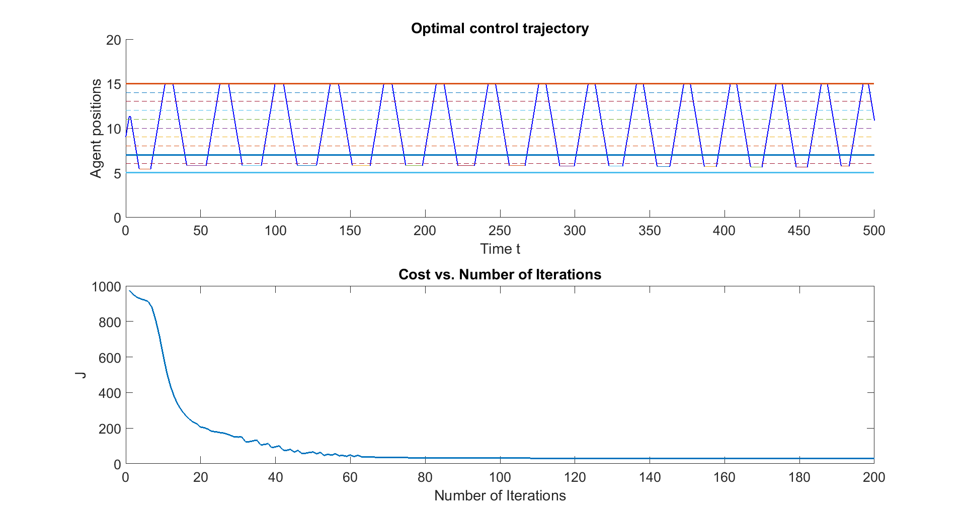
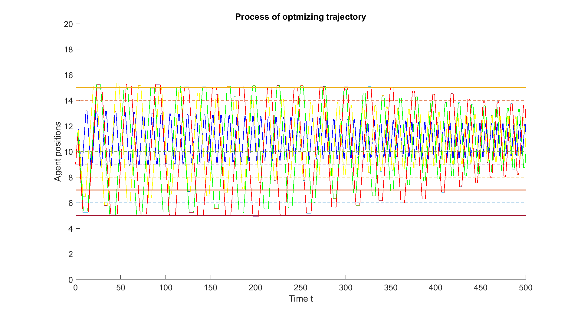
To demonstrate the performance of the gradient-based algorithm using the IPA scheme described in Sec. IV, we present two sets of numerical examples. The first set uses deterministic target locations and dynamics. The results are compared against the optimal found by the discrete scheduling algorithm of Sec. V. The second set demonstrates the robustness of the IPA scheme with respect to a stochastic uncertainty model.

The first simulation consists of a single agent performing a persistent monitoring task on three targets over a time horizon of 100 seconds. The targets are located at positions x1=5,subscript𝑥15x_{1}=5, x2=10,subscript𝑥210x_{2}=10, x3=15subscript𝑥315x_{3}=15 and their uncertainty dynamics in (5) are defined by the parameters Ai=1subscript𝐴𝑖1A_{i}=1, Bi=5subscript𝐵𝑖5B_{i}=5, and Ri(0)=1subscript𝑅𝑖01R_{i}(0)=1 for all i𝑖i. The agent has a sensing range of 2 and is initialized with s(0)=0𝑠00s(0)=0, u(0)=1𝑢01u(0)=1. The results from the IPA gradient descent approach are shown in Fig. 4. The top image shows the optimal trajectory of the agent determined after 1000 iterations of the IPA gradient descent while the bottom shows the evolution of the overall cost as a function of iteration number. The agent is moving through a periodic cycle of x1x2x3x2x1subscript𝑥1subscript𝑥2subscript𝑥3subscript𝑥2subscript𝑥1x_{1}\rightarrow x_{2}\rightarrow x_{3}\rightarrow x_{2}\rightarrow x_{1}\cdots, dwelling for a short time at each target before moving to the next. Notice that the agent dwells for a shorter time at the center target since it visits that location twice per cycle. The second image in the figure shows that gradient descent converges within the first 100 iterations. This simulation aims to test the event driven IPA scheme with the discrete scheduling algorithm which yields optimal but suffers from computational intensity. Thus, we start with a short time horizon T=100𝑇100T=100s. Event-driven IPA optimizes the trajectory fast but the convergence is somewhat unstable due to the lack of events within a short time horizon. The final cost is 26.11. The bottom images in Fig. 4 show the evolution of the target uncertainties.
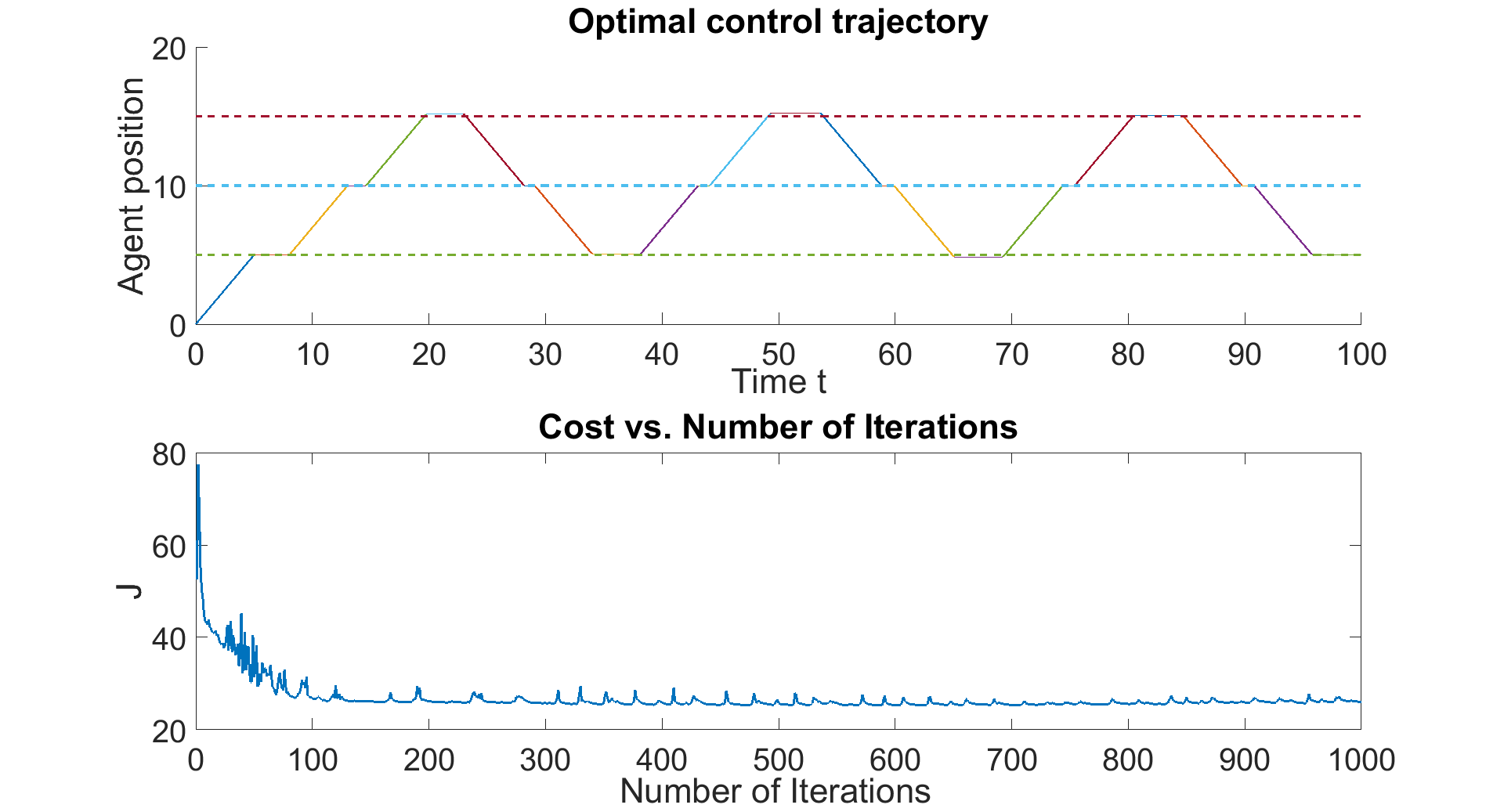
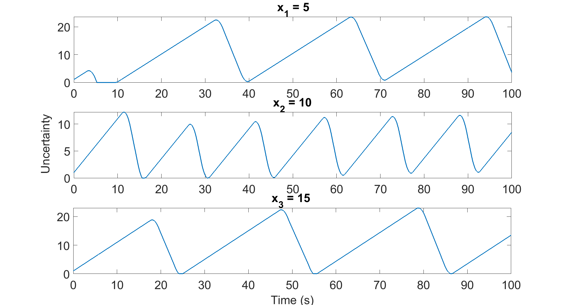
Refer to caption
Refer to caption
Figure 4: A single agent monitoring three targets using the IPA-driven gradient descent algorithm. (top image) Agent trajectory. (second image) Calculated cost as a function of iteration in the gradient descent. The final cost is 26.11. (bottom images) Target uncertainties along the trajectory.

The corresponding result based on the discrete setting of Sec. V is essentially the same with the agent moving through the three targets in a periodic fashion as shown in Fig. 5. The only deviation from the IPA scheme occurs at the end of the horizon where the discrete approach returns to the center target. The final cost was 25.07, matching that of the IPA approach and thus verifying the approximate optimality of the solution found in Fig. 4.

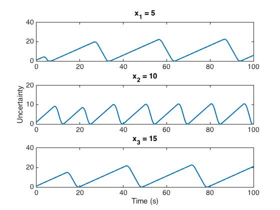
Refer to caption
Refer to caption
Figure 5: A single agent monitoring three targets using the optimal discrete assignment and dwelling time. The final cost is 25.07. (top image) The agent trajectory is almost the same as in Fig. 4. (bottom images) Target uncertainties along the trajectory.

The next simulation involves two agents and five targets over a time horizon of 500 seconds. The targets are located at x1=5,subscript𝑥15x_{1}=5, x2=7,subscript𝑥27x_{2}=7, x3=9,subscript𝑥39x_{3}=9, x4=13,subscript𝑥413x_{4}=13, x5=15subscript𝑥515x_{5}=15. The uncertain dynamics were the same as in the single agent, three target case. As before, the agents have a sensing range of 2 and are initialized at s1(0)=s2(0)=0,subscript𝑠10subscript𝑠200s_{1}(0)=s_{2}(0)=0, with u1(0)=u2(0)=1subscript𝑢10subscript𝑢201u_{1}(0)=u_{2}(0)=1. The results from the event-driven IPA gradient descent approach are shown in Fig. 6. The solution is again periodic with the agents dividing the targets into two groups. Notice that the single agent on targets x4subscript𝑥4x_{4} and x5subscript𝑥5x_{5} is able to keep the uncertainties very close to zero since the targets are quite close relative to the sensing range of the agent. The other agent is able to hold its middle target (x2subscript𝑥2x_{2}) close to zero since it is visited more often. The uncertainties of targets x1subscript𝑥1x_{1} and x3subscript𝑥3x_{3} rise and decrease to zero constantly. The corresponding result based on the discrete setting is shown in Fig. 7. Rather than solve over the full horizon, the problem was solved over a 60 second horizon and then the periodic trajectory repeated to fill the 500 second horizon. The results are again very close to the event-driven IPA method.

Note that the optimal trajectories in both one and two agent examples are bounded between [5,15]515[5,15] (positions of the first and last target), which is consistent with Proposition 1.
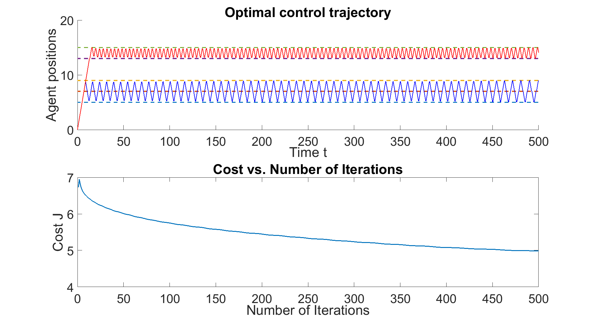
Refer to caption
Refer to caption
Figure 6: Two agents monitoring five targets using the IPA gradient descent algorithm. (top image) Agent trajectories. (second image) Calculated cost as a function of iteration. The final cost is 4.99. (bottom images) Target uncertainty values along the above trajectories.
Refer to caption
Refer to caption
Figure 7: Two agents monitoring five targets using the discrete assignment and dwelling time. The final cost was 4.92. (top image) Agent trajectories. (bottom images) Target uncertainty values along the above trajectories.

As mentioned earlier, the IPA robustness property allows us to handle stochastic uncertainty models at targets. We show a one-agent example in Fig. 8(b) where the uncertainty inflow rate Ai(t)subscript𝐴𝑖𝑡A_{i}(t) is uniformly distributed between [0,2]02[0,2] for all targets. In Fig. 8(c), we introduce randomness by allowing target positions to vary uniformly over [xi0.25,xi+0.25]subscript𝑥𝑖0.25subscript𝑥𝑖0.25[x_{i}-0.25,x_{i}+0.25]. In both cases, the optimal cost in the stochastic models in Figs. 8(b) and 8(c) are close to the optimal cost of the deterministic case Fig. 8(a) where the parameter Aisubscript𝐴𝑖A_{i} and target positions xisubscript𝑥𝑖x_{i} are the means of the associated random processes in the stochastic models. As expected, the convergence depends on the variance of these random processes.

The event excitation issue is addressed in Fig. 9(a), where the agent trajectory is initialized so that it is not close to any of the targets. Using the original problem formulation (without the inclusion of J2(𝜽,𝝎,t)subscript𝐽2𝜽𝝎𝑡J_{2}(\bm{\theta},\bm{\omega},t) in (39), the initial trajectory and cost remain unchanged. After adding J2(𝜽,𝝎,t)subscript𝐽2𝜽𝝎𝑡J_{2}(\bm{\theta},\bm{\omega},t), the blue, green, and red curves in Fig. 9(c) show the trajectory adjustment after 5, 10, and 15 iterations respectively. After 100 iterations, the cost converges to 30.24 as shown in Fig. 9(b) which is close to the optimal cost in Fig. 8(a) where the target dynamics are the same.
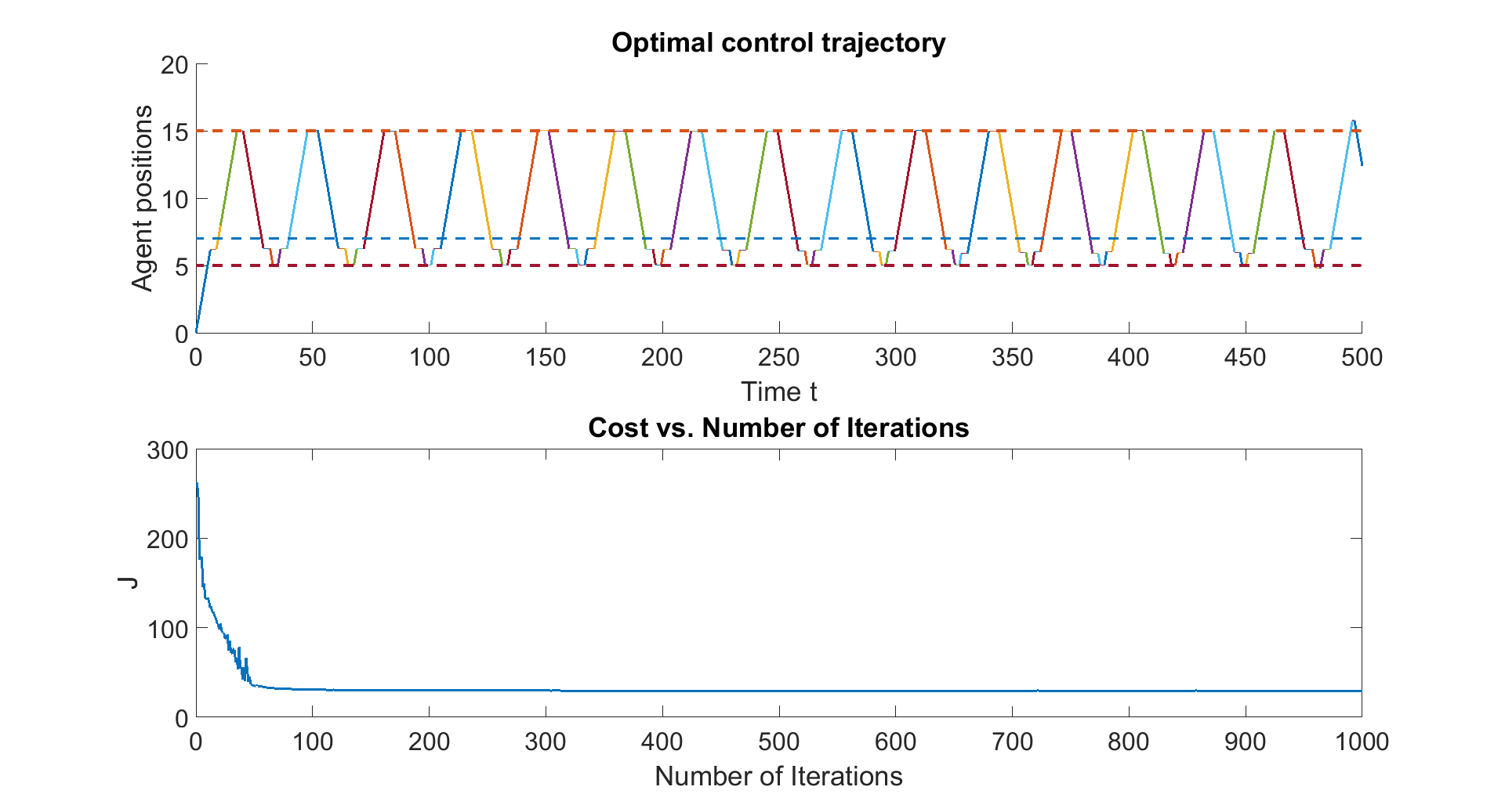
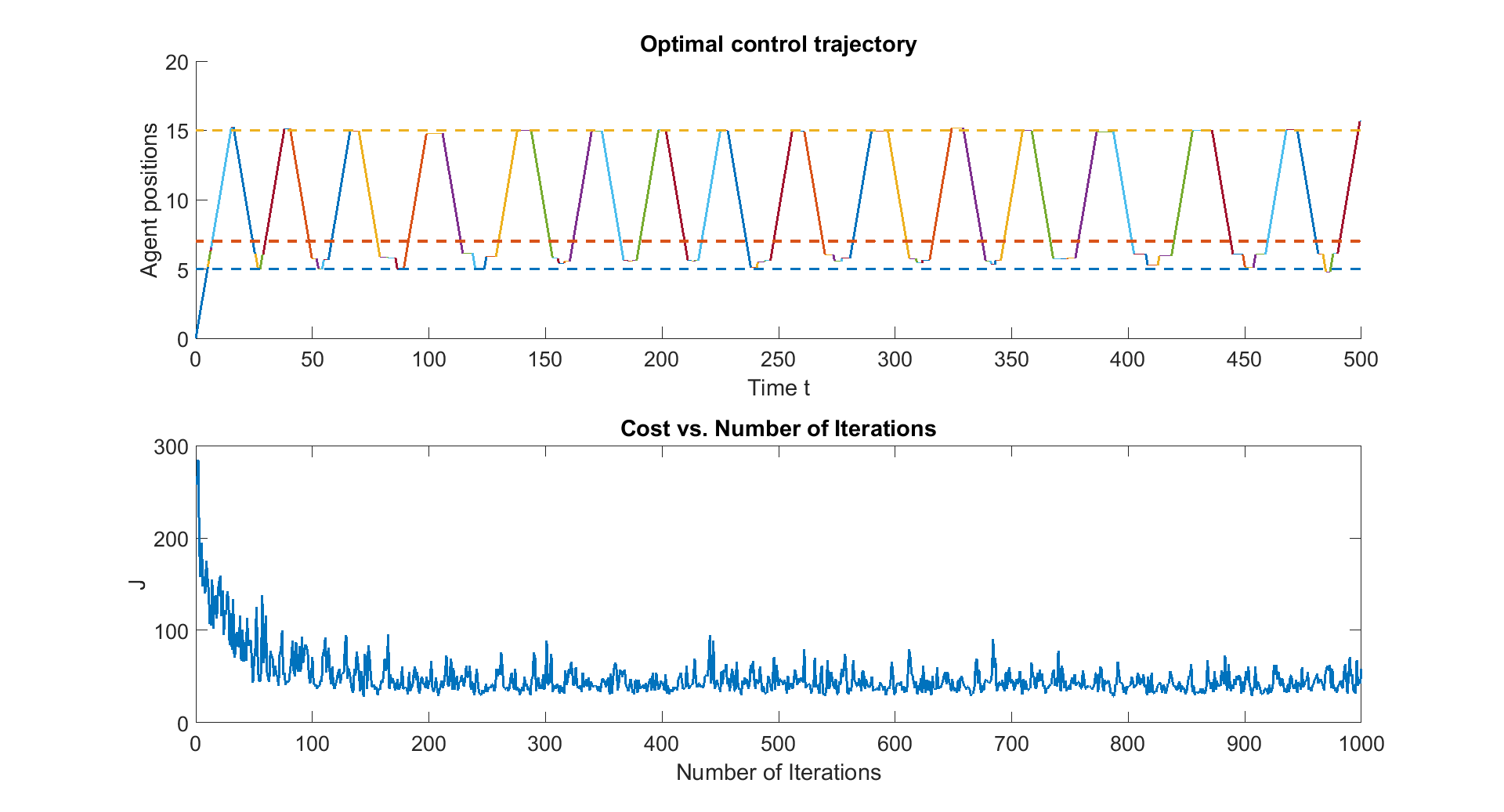
Refer to caption
(a) Example of deterministic target model. Target positions 5,7,1557155,7,15, dynamics parameter Ai=1,B=5,r=2formulae-sequencesubscript𝐴𝑖1formulae-sequence𝐵5𝑟2A_{i}=1,B=5,r=2. J(𝜽,𝝎)=29.40superscript𝐽𝜽𝝎29.40J^{*}(\bm{\theta},\bm{\omega})=29.40.
Refer to caption
(b) Example with stochastic uncertainty processes. AiU(0,2)similar-tosubscript𝐴𝑖𝑈02A_{i}\sim U(0,2). J(𝜽,𝝎)=42.46superscript𝐽𝜽𝝎42.46J^{\ast}(\bm{\theta},\bm{\omega})=42.46.
Refer to caption
(c) Example with stochastic target locations U(xi0.25,xi+0.25)similar-toabsent𝑈subscript𝑥𝑖0.25subscript𝑥𝑖0.25\sim U(x_{i}-0.25,x_{i}+0.25). J(𝜽,𝝎)=34.89superscript𝐽𝜽𝝎34.89J^{\ast}(\bm{\theta},\bm{\omega})=34.89.
Figure 8: Examples demonstrating IPA robustness with respect to stochastic uncertainty. (a)(b)(c) Top plot: optimal trajectory s(t)superscript𝑠𝑡s^{\ast}(t). Bottom plot: cost convergence.
Refer to caption
(a) A trajectory where IPA fails due to lack of event excitation. Top plot: agent trajectory. Bottom plot: cost convergence.
Refer to caption
(b) IPA optimization after event excitation. Top plot: optimal agent trajectory. Bottom plot: cost convergence. J(𝜽,𝝎)=30.24superscript𝐽𝜽𝝎30.24J^{\ast}(\bm{\theta},\bm{\omega})=30.24.
Refer to caption
(c) Trajectory adjustments with event excitation after 5 (blue), 10 (green), and 15 (red) iterations.
Figure 9: The event excitation issue. After adding J2(𝜽,𝝎,t)subscript𝐽2𝜽𝝎𝑡J_{2}(\bm{\theta},\bm{\omega},t), the trajectory adjusts to include targets, the cost converges to 30.24 which is close to the optimal cost in Fig.8(a) where the target dynamics are the same.
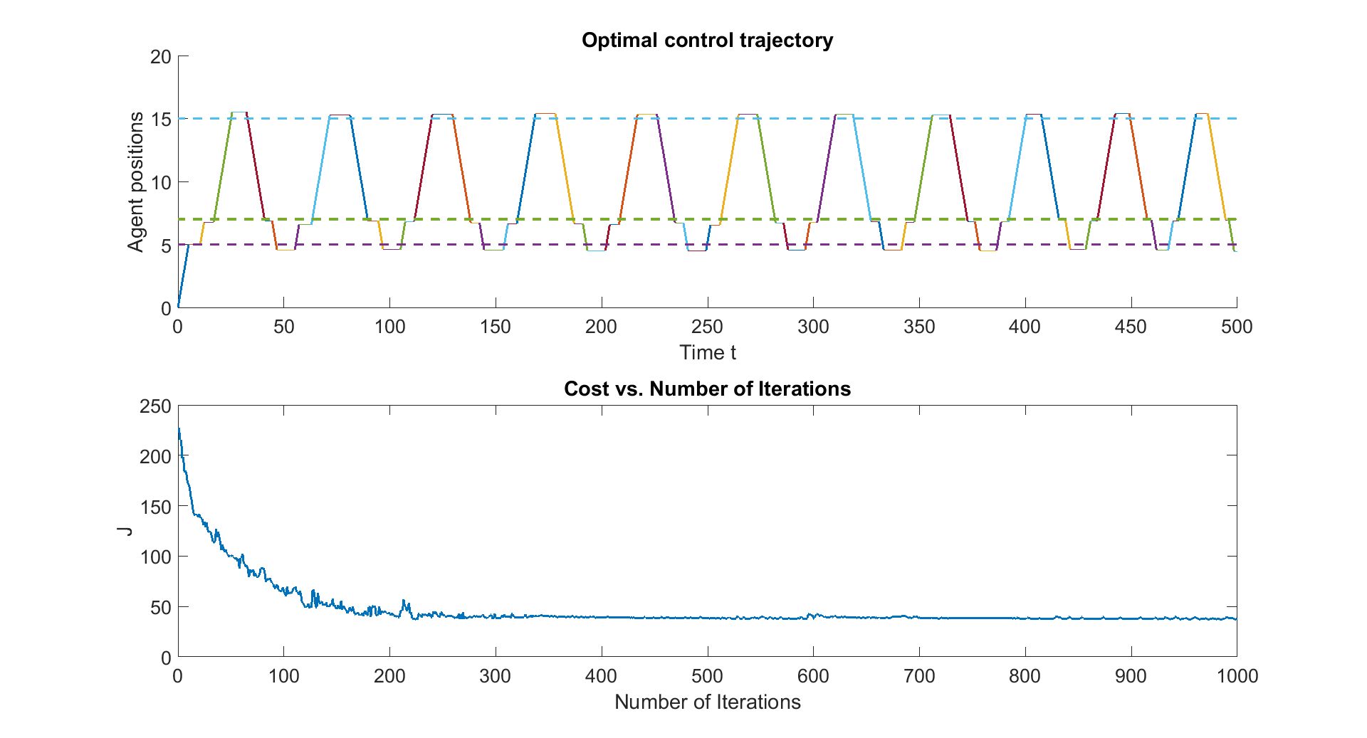
VII Conclusion

We have formulated a persistent monitoring problem with the objective of controlling the movement of multiple cooperating agents so as to minimize an uncertainty metric associated with a finite number of targets. We have established properties of the optimal control solution which reduce the problem to a parametric optimization one. A complete on-line solution is given by Infinitesimal Perturbation Analysis (IPA) to evaluate the gradient of the objective function with respect to all parameters. We also address the case when IPA gradient estimation fails because of the lack of event excitation. We solve this problem by proposing a new metric for the objective function which creates a potential field guaranteeing that gradient values are non-zero. This approach is compared to an alternative graph-based task scheduling algorithm for determining an optimal sequence of target visits. Ongoing research is investigating how to extend these methodologies to higher dimensional mission spaces.

References

  • [1] M. Zhong and C. G. Cassandras, “Distributed coverage control and data collection with mobile sensor networks,” Automatic Control, IEEE Transactions on, vol. 56, no. 10, pp. 2445–2455, 2011.
  • [2] X. Sun and C. G. Cassandras, “Optimal dynamic formation control of multi-agent systems in environments with obstacles,” arXiv preprint arXiv:1508.04727, 2015.
  • [3] C. Cassandras, X. Lin, and X. Ding, “An optimal control approach to the multi-agent persistent monitoring problem,” IEEE Transactions on Automatic Control, vol. 58, no. 4, pp. 947–961, 2013.
  • [4] X. Lin and C. Cassandras, “An optimal control approach to the multi-agent persistent monitoring problem in two-dimensional spaces,” in Proc. of the IEEE Conference on Decision and Control.   IEEE, 2013, pp. 6886–6891.
  • [5] N. Michael, E. Stump, and K. Mohta, “Persistent surveillance with a team of mavs,” in 2011 IEEE/RSJ International Conference on Intelligent Robots and Systems, 2011.
  • [6] S. L. Smith, M. Schwager, and D. Rus, “Persistent monitoring of changing environments using a robot with limited range sensing,” in Proc. of the IEEE International Conference on Robotics and Automation (ICRA).   IEEE, 2011, pp. 5448–5455.
  • [7] Z. Shen and S. B. Andersson, “Tracking Nanometer-Scale Fluorescent Particles in Two Dimensions With a Confocal Microscope,” IEEE Transactions on Control Systems Technology, vol. 19, no. 5, pp. 1269–1278, Sep. 2011.
  • [8] S. M. Cromer Berman, P. Walczak, and J. W. Bulte, “Tracking stem cells using magnetic nanoparticles,” Wiley Interdisciplinary Reviews: Nanomedicine and Nanobiotechnology, vol. 3, no. 4, pp. 343–355, 2011.
  • [9] B. Horling and V. Lesser, “A survey of multi-agent organizational paradigms,” The Knowledge Engineering Review, vol. 19, no. 04, pp. 281–316, 2004.
  • [10] J. Yu, S. Karaman, and D. Rus, “Persistent monitoring of events with stochastic arrivals at multiple stations,” Robotics, IEEE Transactions on, vol. 31, no. 3, pp. 521–535, 2015.
  • [11] E. Stump and N. Michael, “Multi-robot persistent surveillance planning as a vehicle routing problem,” in Automation Science and Engineering (CASE), 2011 IEEE Conference on.   IEEE, 2011, pp. 569–575.
  • [12] C. G. Cassandras, Y. Wardi, C. G. Panayiotou, and C. Yao, “Perturbation analysis and optimization of stochastic hybrid systems,” European Journal of Control, vol. 16, no. 6, pp. 642–661, 2010.
  • [13] Y. Wardi, R. Adams, and B. Melamed, “A unified approach to infinitesimal perturbation analysis in stochastic flow models: the single-stage case,” Automatic Control, IEEE Transactions on, vol. 55, no. 1, pp. 89–103, 2010.
  • [14] M. Schwager, D. Rus, and J.-J. Slotine, “Decentralized, adaptive coverage control for networked robots,” The International Journal of Robotics Research, vol. 28, no. 3, pp. 357–375, 2009.
  • [15] M. Cao, A. S. Morse, C. Yu, B. Anderson, S. Dasgupta et al., “Maintaining a directed, triangular formation of mobile autonomous agents,” Communications in Information and Systems, vol. 11, no. 1, p. 1, 2011.
  • [16] K.-K. Oh and H.-S. Ahn, “Formation control and network localization via orientation alignment,” Automatic Control, IEEE Transactions on, vol. 59, no. 2, pp. 540–545, 2014.
  • [17] Y. Khazaeni and C. G. Cassandras, “Event excitation for event-driven control and optimization of multi-agent systems,” in IEEE International Workshop on Discrete Event Systems(WODES).   IEEE, 2016.
  • [18] A. E. Bryson, Applied optimal control: optimization, estimation and control.   CRC Press, 1975.
  • [19] X. Lan and M. Schwager, “Planning periodic persistent monitoring trajectories for sensing robots in gaussian random fields,” in IEEE International Conference on Robotics and Automation (ICRA).   IEEE, 2013, pp. 2415–2420.
  • [20] M. Lahijanian, J. Wasniewski, S. B. Andersson, and C. Belta, “Motion planning and control from temporal logic specifications with probabilistic satisfaction guarantees,” in IEEE International Conference on Robotics and Automation (ICRA).   IEEE, 2010, pp. 3227–3232.
  • [21] S. L. Smith, J. Tumova, C. Belta, and D. Rus, “Optimal path planning for surveillance with temporal logic constraints,” The International Journal of Robotics Research, p. 0278364911417911, 2011.
  • [22] N. Mathew, S. L. Smith, and S. L. Waslander, “A graph-based approach to multi-robot rendezvous for recharging in persistent tasks,” in Robotics and Automation (ICRA), 2013 IEEE International Conference on.   IEEE, 2013, pp. 3497–3502.
  • [23] X. Yu and S. B. Andersson, “Effect of switching delay on a networked control system,” in Proc.of the IEEE Conference on Decision and Control (CDC).   IEEE, 2013, pp. 5945–5950.
  • [24] X. Yu and S. B. Andersson, “Preservation of system properties for networked linear, time-invariant control systems in the presence of switching delays,” in Proc. of the IEEE Conference on Decision and Control.   IEEE, 2014, pp. 5260–5265.