megaman: Manifold Learning with Millions of points

Abstract

Manifold Learning (ML) is a class of algorithms seeking a low-dimensional non-linear representation of high-dimensional data. Thus ML algorithms are, at least in theory, most applicable to high-dimensional data and sample sizes to enable accurate estimation of the manifold. Despite this, most existing manifold learning implementations are not particularly scalable. Here we present a Python package that implements a variety of manifold learning algorithms in a modular and scalable fashion, using fast approximate neighbors searches and fast sparse eigendecompositions. The package incorporates theoretical advances in manifold learning, such as the unbiased Laplacian estimator introduced by Coifman and Lafon (2006) and the estimation of the embedding distortion by the Riemannian metric method introduced by Perraul-Joncas and Meila (2013). In benchmarks, even on a single-core desktop computer, our code embeds millions of data points in minutes, and takes just 200 minutes to embed the main sample of galaxy spectra from the Sloan Digital Sky Survey — consisting of 0.6 million samples in 3750-dimensions — a task which has not previously been possible.

Keywords: Manifold Learning, Dimension Reduction, Riemannian metric, Graph Embedding, Scalable Methods, Python

1 Motivation

Manifold Learning (ML) algorithms like Diffusion Maps or Isomap find a non-linear representation of high-dimensional data with a small number of dimensions. Research in ML is making steady progress, yet there is currently no ML software library efficient enough to be used in realistic research and application of ML.

The first comprehensive attempt to bring several manifold learning algorithms under the same umbrella is the mani Matlab package authored by Wittman (2010). This package was instrumental in illustrating the behavior of the existing ML algorithms of a variety of synthetic toy data sets. More recently, a new Matlab toolbox drtoolbox was released, that implements over thirty dimension reduction methods, and works well with sample sizes in the thousands.

Perhaps the best known open implementation of common manifold learning algorithms is the manifold sub-module of the Python package scikit-learn (Pedregosa et al., 2011). This software benefits from the integration with scikit-learn, meets its standards and philosophy, comes with excellent documentation and examples, and is written in a widely supported open language.

The scikit-learn package strives primarily for usability rather than scalability. While the package does feature some algorithms designed with scalability in mind, the manifold methods are not among them. For example, in scikit-learn it is difficult for different methods to share intermediate results, such as eigenvector computations, which can lead to inefficiency in data exploration. The scikit-learn manifold methods cannot handle out-of-core data, which leads to difficulties in scaling. Moreover, though scikit-learn accepts sparse inputs and uses sparse data structures internally, the current implementation does not always fully exploit the data sparsity.

To address these challenges, we propose megaman, a new Python package for scalable manifold learning. This package is designed for performance, while adopting the look and feel of the scikit-learn package, and inheriting the functionality of scikit-learn’s well-designed API (Buitinck et al., 2013).

2 Background on non-linear dimension reduction and manifold learning

This section provides a brief description of non-linear dimension reduction via manifold learning, outlining the tasks performed by a generic manifold learning algorithm. The reader can find more information on this topic in Perraul-Joncas and Meila (2013), as well as on the scikit-learn web site.

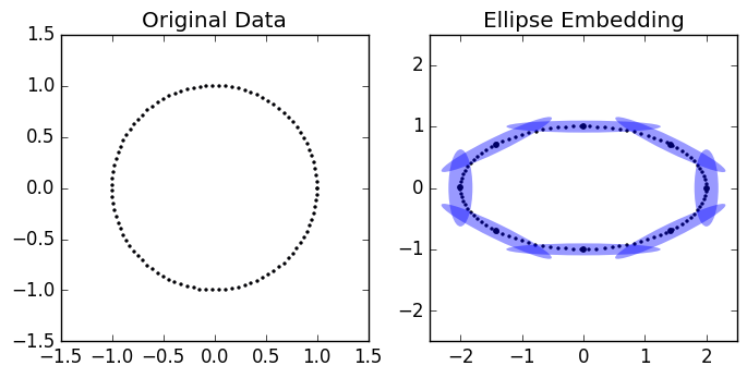
We assume that a set of $N$ vectors $x_{1},\ldots x_{N}$ in $D$ dimensions is given (for instance, for the data in Figure 5, $N=3\times 10^{6},\,D=300$). It is assumed that these data are sampled from (or approximately from) a lower dimensional space (i.e. a manifold) of intrinsic dimension $d$. The goal of manifold learning is to map the vectors $x_{1},\ldots x_{N}$ to $s$-dimensional vectors $y_{1},\ldots y_{N}$, where $y_{i}$ is called the embedding of $x_{i}$ and $s\ll D,\,s\geq d$ is called the embedding dimension. The mapping should preserve the neighborhood relations of the original data points, and as much as possible of their local geometric relations.

From the point of view of a ML algorithm (also called an embedding algorithm), non-linear dimension reduction subsumes the following stages.

Constructing a neighborhood graph $G$, that connects all point pairs $x_{i},x_{j}$ which are “neighbors”. The graph $G$ is sparse when data can be represented in low dimensions. From this graph, a similarity $S_{ij}\geq 0$ between any pair of points $x_{i},x_{j}$ is computed by $S_{ij}=\exp\left(-||x_{i}-x_{j}||^{2}/\sigma^{2}\right)$, where $\sigma$ is a user-defined parameter controlling the neighborhood size. This leads to a $N\times N$ similarity matrix $S$, sparse. Constructing the neighborhood graph is common to most existing ML algorithms.

From $S$ a special $N\times N$ symmetric matrix called the Laplacian is derived. The Laplacian is directly used for embedding in methods such as the Spectral Embedding (also known as Laplacian Eigenmaps) of Belkin and Niyogi (2002) and Diffusion Maps of Nadler et al. (2006). The Laplacian is also used after embedding, in the post-processing stage. Because these operations are common to many ML algorithms and capture the geometry of the high-dimensional data in the matrices $S$ or $L$, we will generically call the software modules that implement them Geometry.

The next stage, the Embedding proper, can be performed by different embedding algorithms. An embedding algorithm take as input a matrix, which can be either the matrix of distances $||x_{i}-x_{j}||$ or a matrix derived from it, such as $S$ or $L$. Well known algorithms implemented by megaman are Laplacian Eigenmaps (Belkin and Niyogi, 2002), Diffusion Maps (Nadler et al., 2006), Isomap (Bernstein et al., 2000), etc. The ouput of this step is the $s$-dimensional representation $y_{i}$ corresponding to each data point $x_{i}$. Embedding typically involves computing ${\cal O}(d)$ eigenvectors of some $N\times N$ matrix. To note that this matrix has the same sparsity pattern as the neighborhood graph $G$.

Figure 1: megaman classes (gray, framed), packages (gray, no frame) and external packages (blue). The class structure reflects the relationships between ML tasks.

Finally, for a given embedding $y_{1},\ldots y_{n}$, one may wish to estimate the distortion incurred w.r.t the original data. This can be done via the method of Perraul-Joncas and Meila (2013), by calculating for each point $y_{i}$ a metric $R_{i}$; $R_{i}$ is an $s\times s$ symmetric, positive definite matrix. Practically, the value $u^{T}R_{i}u$, with $u$ a unit vector, is the “stretch” at $y_{i}$ in direction $u$ of the embedding $\{y_{1},\ldots,y_{N}\}$ w.r.t the original data $\{x_{1},\ldots x_{N}\}$. In particular, for an embedding with no stretch, $R_{i}$ should be equal to the unit matrix. The metric given by $R_{1},\ldots R_{N}$ can be used to calculate distances, areas and volumes using the embedded data, which approximate well their respective values on the original high-dimensional data. Therefore, obtaining $R_{1:N}$ along with the embedding coordinates $y_{1:N}$ provides a geometry-preserving (lossy) compression of the original $x_{1:N}$.

The logical structure of these tasks is shown in Figure 1, along with some of the classes and software packages used to implement them.

Figure 2: The circle on the left hand plot represents the original data with $D=2$. The ellipse in the right hand plot is an “embedding” of these data into $s=2$ dimensions, which deforms the circle into an ellipse. The blue ovals plotted at selected points represent the (dual) Riemannian Metric at that point. The long axes of the ellipses represent the local unit of length along the ellipse ; the units are smaller left and right, where the length of the original curve was compressed, and larger in the middle where the circle was stretched.

3 Software design

3.1 Functionality

We provide classes that implement the above tasks, along with post-processing and visualization tools. The package implements recent advances in the statistical understanding of manifold learning such as:

• It has been shown decisively by Hein et al. (2007) and Ting et al. (2010) that the construction of the neighborhood graph can influence the resulting embedding. In particular, the $k$-nearest neighbor graph construction introduces biases that can be avoided by the use of the $\epsilon$-radius graphs. Therefore, the default graph construction method is radius_neighbors.

• A variety of graph Laplacians (unnormalized, normalized, random_walk (von Luxburg, 2007), renormalized and geometric (Coifman and Lafon, 2006)) are available. The default choice is the geometric Laplacian introduced by (Coifman and Lafon, 2006) who showed that this choice eliminates the biases due variation in the density of the samples.

• Embedding metric estimation following Perraul-Joncas and Meila (2013). The (dual) Riemannian metric measures the “stretch” introduced by the embedding algorithm with respect to the original data; Figure 2 illustrates this.

3.2 Designed for performance

The megaman package is designed to be simple to use with an interface that is similar to the popular scikit-learn python package. Additionally, megaman is designed with experimental and exploratory research in mind.

3.2.1 Computational challenges

The ML pipeline described above and in Figure 1 comprises two significant computational bottlenecks.

Computing the neighborhood graph involves finding the $K$-nearest neighbors, or the $r$-nearest neighbors (i.e all neighbors within radius $r$) in $D$ dimensions, for $N$ data points. This leads to sparse graph $G$ and sparse $N\times N$ matrix $S$ with ${\cal O}(d)$ neighbors per node, respectively entries per row. All $N\times N$ matrices in subsequent steps will have the same sparsity pattern as $S$. Naively implemented, this computation requires ${\cal O}(N^{2}(D+\log N))$ operations.

Eigendecomposition A large number of embedding algorithms (effectively all algorithms implemented in megaman) involve computing ${\cal O}(s)$ principal eigenvectors of an $N\times N$ symmetric, semi-positive definite matrix. This computation scales like ${\cal O}(N^{2}s)$ for dense matrices. In addition, if the working matrices were stored in dense form, the memory requirements would scale like $N^{2}$, and elementary linear algebra operations like matrix-vector multiplications would scale likewise.

3.2.2 Main design features

We made several design and implementation choices in support of scalability.

• Sparse representation are used as default for optimal storage and computations.

• We incorporated state of the art Fast Library Approximate Nearest Neighbor search algorithm by Muja and Lowe (2014) (can handle Billions of data points) with a cython interface to Python allowing for rapid neighbors computation.

• Intermediate data structures (such as data set index, distances, affinity matrices, Laplacian) are cached allowing for testing alternate parameters and methods without redundant computations.

• By converting matrices to sparse symmetric positive definite (SSPD) in all cases, megaman takes advantage of pyamg and of the Locally Optimal Block Preconditioned Conjugate Gradient (LOBPCG) package as a matrix-free method (Knyazev, 2001) for solving generalized eigenvalue problem for SSPD matrices. Converting to symmetric matrices also improves the numerical stability of the algorithms.

With these, megaman runs in reasonable time on data sets in the millions. The design also supports well the exploratory type of work in which a user experiments with different parameters (e.g. radius or bandwidth parameters) as well as different embedding procedures; megaman caches any re-usable information in both the Geometry and embedding classes.

3.3 Designed for extensions

megaman’s interface is similar to that of the scikit-learn package, in order to facilitation easy transition for the users of scikit-learn.

megaman is object-oriented and modular. For example, the Geometry class provides user access to geometric computational procedures (e.g. fast approximate radius neighbors, sparse affinity and Laplacian construction) as an independent module, whether the user intends to use embedding methods or not. megaman also offers the unified interface eigendecomposition to a handful of different eigendecomposition procedures (dense, arpack, lobpcg, amg). Consequently, the megaman package can be used for access to these (fast) tools without using the other classes. For example, megaman methods can be used to perform the Laplacian computation and embedding steps of spectral clustering. Finally, Geometry accepts input in a variety of forms, from data cloud to similarity matrix, allowing a user to optionally input a precomputed similarity.

This design facilitates easy extension of megaman’s functionality. In particular, new embedding algorithms and new methods for distance computation can be added seamlessly. More ambitious possible extensions are: neighborhood size estimation, dimension estimation, Gaussian process regression.

Finally, the megaman package also has a comprehensive documentation with examples and unit tests that can be run with nosetests to ensure validity. To allow future extensions megaman also uses Travis Continuous Integration.

4 Downloading and installation

megaman is publically available at: https://github.com/mmp2/megaman. megaman’s required dependencies are numpy, scipy, and scikit-learn, but for optimal performance FLANN, cython, pyamg and a c compiler gcc are also required. For unit tests and integration megaman depends on nose. The most recent megaman release can be installed along with its dependencies using the cross-platform conda package manager:

⬇

$ conda install -c https://conda.anaconda.org/jakevdp megaman

Alternatively, the megaman can be installed from source by downloading the source repository and running:

⬇

$ python setup.py install

With nosetests installed, unit tests can be run with:

⬇

$ make test

5 Quick start

For full documentation see the megaman website at: http://mmp2.github.io/megaman/

⬇

from megaman.geometry import Geometry

from megaman.embedding import SpectralEmbedding

from sklearn.datasets import make_swiss_roll

n = 10000

X, t = make_swiss_roll( n )

n_components = 2

radius = 1.1

geom = Geometry(adjacency_method = ’cyflann’,

adjacency_kwds = {’radius’:radius},

affinity_method = ’gaussian’,

affinity_kwds = {’radius’:radius},

laplacian_method = ’geometric’,

laplacian_kwds = {’scaling_epps’:radius})

SE = SpectralEmbedding(n_components=n_components,

eigen_solver=’amg’,

geom=geom)

embed_spectral = SE.fit_transform(X)

6 Classes overview

The following is an overview of the classes and other tools provided in the megaman package:

Geometry This is the primary non-embedding class of the package. It contains functions to compute the pairwise distance matrix (interfacing with the distance module), the Gaussian kernel similarity matrix $S$ and the Laplacian matrix $L$. A Geometry object is what is passed or created inside the embedding classes.

RiemannianMetric This class produces the estimated Riemannian metric $R_{i}$ at each point $i$ given an embedding $y_{1:N}$ and the estimated Laplacian from the original data.

embeddings The manifold learning algorithms are implemented in their own classes inheriting from a base class. Included are:

• SpectralEmbedding implements Laplacian Eigenmaps (Belkin and Niyogi, 2002) and Diffusion Maps (Nadler et al., 2006): These methods use the eigendecomposition of the Laplacian.

• LTSA implements the Local Tangent Space Alignment method (Zhang and Zha, 2004): This method aligns estimates of local tangent spaces.

• LocallyLinearEmbedding (LLE) (Roweis and Saul, 2000): This method finds embeddings that preserve local reconstruction weights

• Isomap (Bernstein et al., 2000): This method uses Multidimensional Scaling to preserve shortest-path distances along a neighborhood-based graph.

eigendecomposition Not implemented as a class, this module provides a unified (function) interface to the different eigendecomposition methods provided in scipy. It also provides a null space function (used by LLE and LTSA).

7 Benchmarks

Figure 3: Run time vs. data set size $N$ for fixed $D=100$ and $\epsilon=\frac{5}{N^{1/8}}+D^{1/4}-2$. The data is from a Swiss Roll (in 3 dimensions) with an additional 97 noise dimensions, embedded into $s=2$ dimensions by the spectral_embedding algorithm. By $N=1,000,000$ scikit-learn was unable to compute an embedding due to insufficient memory. All megaman run times (including time between distance and embedding) are faster than scikit-learn.

Figure 4: Run time vs. data set dimension $D$ for fixed $N=50,000$ and $\epsilon=\frac{5}{N^{1/8}}+D^{1/4}-2$. The data is from a Swiss Roll (in 3 dimensions) with additional noise dimensions, embedded into $s=2$ dimensions by the spectral_embedding algorithm. By $D=10,000$ scikit-learn was unable to compute an embedding due to insufficient memory. All megaman run times (including time between distance and embedding) are faster than scikit-learn.

The one other popular comparable implementation of manifold learning algorithms is the scikit-learn package.

To make the comparison as fair as possible, we choose the Spectral Embedding method for the comparison, because both scikit-learn and megaman allow for similar settings:

• Both are able to use radius-based neighborhoods

• Both are able to use the same fast eigensolver, a Locally-Optimized Block-Preconditioned Conjugate Gradient (lobpcg) using the algebraic multigrid solvers in pyamg.

Incidentally, Spectral Embedding is empirically the fastest of the usual manifold learning methods, and the best understood theoretically. Note that with the default settings, scikit-learn  would perform slower than in our experiments.

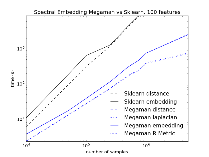
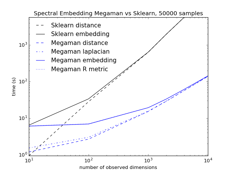
We display total embedding time (including time to compute the graph $G$, the Laplacian matrix and the embedding) for megaman versus scikit-learn, as the number of samples $N$ varies (Figure 3) or the data dimension $D$ varies (Figure 4). All benchmark computations were performed on a single desktop computer running Linux with 24.68GB RAM and a Quad-Core 3.07GHz Intel Xeon CPU. We use a relatively weak machine to demonstrate that our package can be reasonably used without high performance hardware.

The experiments show that megaman scales considerably better than scikit-learn, even in the most favorable conditions for the latter; the memory footprint of megaman is smaller, even when scikit-learn  uses sparse matrices internally. The advantages grow as the data size grows, whether it is w.r.t $D$ or to $N$.

The two earlier identified bottlenecks, distance computation and eigendecomposition, dominate the compute time. By comparison, the other steps of the pipe-line, such as Laplacian and Riemannian metric computation are negligible. When $D$ is large, the distance computation dominates, while for $N\ll D$, the eigendecomposition takes a time comparatively equal to the distance computation.

Figure 5: 3,000,000 words and phrases mapped by word2vec into 300 dimensions were embedded into 2 dimensions using Spectral Embedding. The plot shows a sample of 10,000 points displaying the overall shape of the embedding as well as the estimated “stretch” (i.e. dual push-forward Riemannian metric) at various locations in the embedding.

Figure 6: A three-dimensional embedding of the main sample of galaxy spectra from the Sloan Digital Sky Survey (approximately 675,000 spectra observed in 3750 dimensions). Colors in the above figure indicate the strength of Hydrogen alpha emission, a very nonlinear feature which requires dozens of dimensions to be captured in a linear embedding (Yip et al., 2004). A nonlinear embedding such as the one shown here is able to capture that information much more succinctly (Vanderplas and Connolly, 2009). (Figure by O. Grace Telford.)

We report run times on two other real world data sets, where the embedding were done solely with megaman. The first is the word2vec data set which contains feature vectors in 300 dimensions for about 3 million words and phrases, extracted from Google News. The vector representation was obtained via a multilayer neural network by Mikolov et al. (2013).

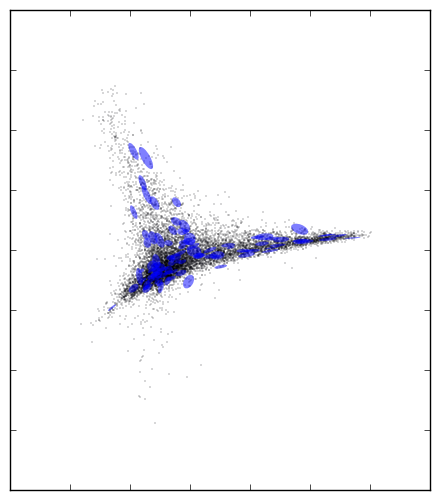
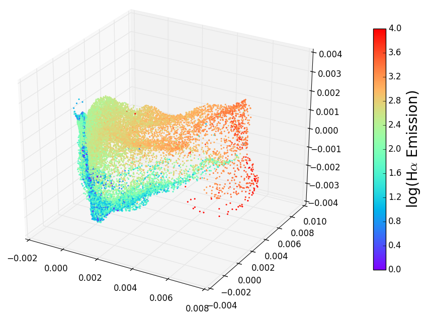
The second data set contains galaxy spectra from the Sloan Digital Sky Survey (Abazajian et al., 2009). We extracted a subset of galaxy spectra whose SNR was sufficiently high, known as the main sample. This set contains fluxes from 675,000 galaxies observed in 3750 spectral bins, preprocessed as described in Telford et al. (2016). Previous manifold learning studies of this data operated on carefully selected subsets of the data in order to circumvent computational difficulties of ML (e.g. Vanderplas and Connolly, 2009). Here for the first time we present a manifold embedding from the entire sample.

			Run time [min]
Dataset	Size $N$	Dimensions $D$	Distances	Embedding	R. metric	Total
Spectral	0.7M	3750	190.5	8.9	0.1	199.5
Word2Vec	3M	300	107.9	44.8	0.6	153.3

8 Conclusion

megaman puts in the hands of scientists and methodologists alike tools that enable them to apply state of the art manifold learning methods to data sets of realistic size. The package is easy to use for all scikit-learn  users, it is extensible and modular. We hope that by providing this package, non-linear dimension reduction will be benefit those who most need it: the practitioners exploring large scientific data sets.

Acknowledgments

We would like to acknowledge support for this project from the National Science Foundation (NSF grant IIS-9988642), the Multidisciplinary Research Program of the Department of Defense (MURI N00014-00-1-0637), the Department of Defense (62-7760 “DOD Unclassified Math”), and the Moore/Sloan Data Science Environment grant. We are grateful to Grace Telford for creating Figure 6. This project grew from the Data Science Incubator program at the University of Washington eScience Institute.

References

- Abazajian et al. (2009) K. N. Abazajian, J. K. Adelman-McCarthy, M. A. Agüeros, S. S. Allam, C. Allende Prieto, D. An, K. S. J. Anderson, S. F. Anderson, J. Annis, N. A. Bahcall, and et al. The Seventh Data Release of the Sloan Digital Sky Survey. Astrophysical Journal Supplement Series, 182:543-558, June 2009. doi: 10.1088/0067-0049/182/2/543.
- Belkin and Niyogi (2002) M. Belkin and P. Niyogi. Laplacian eigenmaps and spectral techniques for embedding and clustering. In T. G. Dietterich, S. Becker, and Z. Ghahramani, editors, Advances in Neural Information Processing Systems 14, Cambridge, MA, 2002. MIT Press.
- Bernstein et al. (2000) Mira Bernstein, Vin de Silva, John C. Langford, and Josh Tennenbaum. Graph approximations to geodesics on embedded manifolds. http://web.mit.edu/cocosci/isomap/BdSLT.pdf, December 2000.
- Buitinck et al. (2013) Lars Buitinck, Gilles Louppe, Mathieu Blondel, Fabian Pedregosa, Andreas Mueller, Olivier Grisel, Vlad Niculae, Peter Prettenhofer, Alexandre Gramfort, Jaques Grobler, et al. API design for machine learning software: experiences from the scikit-learn project. arXiv preprint arXiv:1309.0238, 2013.
- Coifman and Lafon (2006) R. R. Coifman and S. Lafon. Diffusion maps. Applied and Computational Harmonic Analysis, 30(1):5–30, 2006.
- Hein et al. (2007) Matthias Hein, Jean-Yves Audibert, and Ulrike von Luxburg. Graph laplacians and their convergence on random neighborhood graphs. Journal of Machine Learning Research, 8:1325–1368, 2007. URL http://dl.acm.org/citation.cfm?id=1314544.
- Knyazev (2001) Andrew V. Knyazev. Toward the optimal preconditioned eigensolver: Locally optimal block preconditioned conjugate gradient method. SIAM Journal on Scientific Computing, 23(2):517–541, 2001. doi: 10.1137/S1064827500366124. URL http://dx.doi.org/10.1137/S1064827500366124.
- Mikolov et al. (2013) Tomas Mikolov, Ilya Sutskever, Kai Chen, Greg Corrado, and Jeffrey Dean. Distributed representations of words and phrases and their compositionality. In Advances in Neural Information Processing Systems 26, 2013.
- Muja and Lowe (2014) Marius Muja and David G. Lowe. Scalable nearest neighbor algorithms for high dimensional data. Pattern Analysis and Machine Intelligence, IEEE Transactions on, 36, 2014.
- Nadler et al. (2006) Boaz Nadler, Stephane Lafon, Ronald Coifman, and Ioannis Kevrekidis. Diffusion maps, spectral clustering and eigenfunctions of Fokker-Planck operators. In Y. Weiss, B. Schölkopf, and J. Platt, editors, Advances in Neural Information Processing Systems 18, pages 955–962, Cambridge, MA, 2006. MIT Press.
- Pedregosa et al. (2011) Fabian Pedregosa, Gaël Varoquaux, Alexandre Gramfort, Vincent Michel, Bertrand Thirion, Olivier Grisel, Mathieu Blondel, Peter Prettenhofer, Ron Weiss, Vincent Dubourg, et al. Scikit-learn: Machine learning in Python. The Journal of Machine Learning Research, 12:2825–2830, 2011.
- Perraul-Joncas and Meila (2013) D. Perraul-Joncas and M. Meila. Non-linear dimensionality reduction: Riemannian metric estimation and the problem of geometric discovery. ArXiv e-prints, May 2013.
- Roweis and Saul (2000) Sam Roweis and Lawrence Saul. Nonlinear dimensionality reduction by locally linear embedding. Science, 290(5500):2323–2326, December 2000.
- Telford et al. (2016) O. Grace Telford, Jacob Vanderplas, James McQueen, and Marina Meila. Metric embedding of Sloan galaxy spectra. (in preparation), 2016.
- Ting et al. (2010) Daniel Ting, Ling Huang, and Michael I. Jordan. An analysis of the convergence of graph laplacians. In Proceedings of the 27th International Conference on Machine Learning (ICML-10), June 21-24, 2010, Haifa, Israel, pages 1079–1086, 2010. URL http://www.icml2010.org/papers/554.pdf.
- Vanderplas and Connolly (2009) J. Vanderplas and A. Connolly. Reducing the Dimensionality of Data: Locally Linear Embedding of Sloan Galaxy Spectra. Astronomical Journal, 138:1365–1379, November 2009. doi: 10.1088/0004-6256/138/5/1365.
- von Luxburg (2007) Ulrike von Luxburg. A tutorial on spectral clustering. Statistics and Computing, 17(4):395–416, 2007.
- Wittman (2010) T. Wittman. Manifold learning matlab demo. http://www.math.umn.edu/~wittman/mani/, retrieved 07/2010, 2010.
- Yip et al. (2004) C. W. Yip, A. J. Connolly, A. S. Szalay, T. Budavári, M. SubbaRao, J. A. Frieman, R. C. Nichol, A. M. Hopkins, D. G. York, S. Okamura, J. Brinkmann, I. Csabai, A. R. Thakar, M. Fukugita, and Ž. Ivezić. Distributions of Galaxy Spectral Types in the Sloan Digital Sky Survey. Astronomical Journal, 128:585–609, August 2004. doi: 10.1086/422429.
- Zhang and Zha (2004) Zhenyue Zhang and Hongyuan Zha. Principal manifolds and nonlinear dimensionality reduction via tangent space alignment. SIAM J. Scientific Computing, 26(1):313–338, 2004.