IPPP/16/17

Interpreting 750 GeV Diphoton Excess in Plain NMSSM

M. Badziak^a,b, M. Olechowski^a, S. Pokorski^a and K. Sakurai^c

^aInstitute of Theoretical Physics, Faculty of Physics, University of Warsaw

ul. Pasteura 5, PL–02–093 Warsaw, Poland

^bBerkeley Center for Theoretical Physics, Department of Physics,

and Theoretical Physics Group, Lawrence Berkeley National Laboratory,

University of California, Berkeley, CA 94720, USA

^cInstitute for Particle Physics Phenomenology, Department of Physics,

University of Durham, Science Laboratories, South Road, Durham, DH1 3LE, UK

Abstract

NMSSM has enough ingredients to explain the diphoton excess at 750 GeV: singlet-like (pseudo) scalar ($a$) $s$ and higgsinos as heavy vector-like fermions. We consider the production of the 750 GeV singlet-like pseudo scalar $a$ from a decay of the doublet-like pseudo scalar $A$, and the subsequent decay of $a$ into two photons via higgsino loop. We demonstrate that this cascade decay of the NMSSM Higgs bosons can explain the diphoton excess at 750 GeV.

1 Introduction

Recently ATLAS and CMS have reported excesses in the diphoton mass distribution around $m_{\gamma\gamma}\simeq 750$ GeV in their 13 TeV data. The local significance assuming narrow width is $\sim 3.6\,\sigma$ for ATLAS [1] and $\sim 2.6\,\sigma$ for CMS [2]. ATLAS and CMS have presented their updated analyses at Moriond conference. With the improved analyses, the local significance has increased to $\sim 3.9\,\sigma$ and $\sim 3.4\,\sigma$ for ATLAS and CMS, respectively [3, 4]. Fitting that excess with a narrow resonance around 750 GeV, CMS reports for the cross section times branching ratio, $\sigma_{13\rm TeV}\cdot{\rm BR}_{\gamma\gamma}$, the value $2.6\div 7.7$ fb at 1 $\sigma$ and $0.85\div(11-12)$fb at 2 $\sigma$ (see Fig.10 of [4]). The CMS fit of the excess around $m_{\gamma\gamma}\simeq 750$ GeV in the 8 TeV data gives $0.31\div 1.00$ fb at 1-$\sigma$ and $0.06\div 1.45$ fb at 2-$\sigma$ [4]. The ATLAS collaboration has not provided such a detailed analysis for a narrow resonance hypothesis. A fit reported in ref. [5] gives for $\sigma\cdot{\rm BR}_{\gamma\gamma}$ the values $\simeq 4\div 7$ fb and $\simeq 0\div 0.42$ fb at 1 $\sigma$ at 13 TeV and 8 TeV, respectively. No information about the 2 $\sigma$ regions is available.

The possible interpretation and implications of the excess has been intensively studied. Most such studies introduce new particles to account for the excess without asking about their UV origin, and interpretation within the known models in particular Minimal Supersymmetric Starndard Model (MSSM) and Next-to-Minimal Supersymmetric Standard Model (NMSSM) is rare. In this paper we study the possibility to explain the diphoton excess within the framework of NMSSM without introducing additional particles.

One of the most straightforward interpretations of the excess is to consider a direct production of a scalar or pseudoscalar 750 GeV particle, $X$, decaying to two photons: $\alpha\beta\to X\to\gamma\gamma$, where $\alpha$, $\beta$ are the initial state partons. If the model is renormalizable, $X\to\gamma\gamma$ suggests the existence of electrically-charged vector-like fermions (or scalars) coupled to $X$ [10, 11, 12, 13, 14, 15, 16, 17, 18, 19, 20, 21, 22, 23, 24, 25, 26, 27, 28, 29, 30, 31, 32, 33, 34, 35, 36, 37, 38, 39, 40, 41, 42, 43, 44, 45, 46, 47, 48, 49, 50, 51, 52, 53, 54, 55, 56, 57, 58, 59, 60, 61, 62, 63, 64, 65, 66, 67, 68], which generate the effective operator $XF^{\mu\nu}F_{\mu\nu}(\tilde{F}_{\mu\nu})$. Such fermions should be heavier than $m_{X}/2\simeq 375$ GeV, otherwise the diphoton rate is strongly suppressed because $X$ predominantly decays into the vector-like fermions on shell. Similar argument disfavours the possibility to identify $X$ as the heavy higgs bosons in the MSSM or 2HDM, because in such models $X$ predominantly decays into $t\bar{t}$ and/or $b\bar{b}$ [71]. In general, in such scenarios the decay branching ratios of $X$ are strongly correlated with the production cross section.

Another possibility is to consider the production of $X$ from a decay of a heavy resonance $Y_{r}$ associated with another particle $Y_{d}$: $\alpha\beta\to Y_{r}\to Y_{d}X$, $X\to\gamma\gamma$ [10, 72, 73, 74, 75]. This topology has two advantages. First, ${\rm BR}(X\to\gamma\gamma)$ is independent of the production cross section of the resonance. This is not the case for the previous topology, because a large production cross section leads to a large rate of the inverse decay process $X\to\alpha\beta$, which suppresses ${\rm BR}(X\to\gamma\gamma)$. Second, the mass of $Y_{r}$ has to be larger than $m_{X}\simeq 750$ GeV, and the 13 TeV production cross section of $Y_{r}$ is more enhanced with respect to the 8 TeV cross section, compared to the previous topology. In this context we notice that, while there is no big tension between 8 and 13 TeV data in the CMS fits interpreted as a direct production of a 750 GeV resonance, the fit of ref. [5] to the ATLAS data shows such a tension well above 2 $\sigma$ level. For instance, if the initial partons are gluons, $\alpha\beta=gg$, translating the results of that fit for 8 TeV, interpreted as a direct production of the 750 GeV resonance, to 13 TeV clearly shows the problem. Thus, the cascade topology may slightly help to reconcile the ATLAS data at 8 and 13 TeV and the results of both experiments.

This topology can be relatively easily realised in the NMSSM by identifying $Y_{r}=A$, $Y_{d}=s$ and $X=a$: $\alpha\beta\to A\to sa$, $a\to\gamma\gamma$, as shown in Fig. 1, where $A$ is the doublet-like pseudo scalar and ($a$) $s$ is the singlet-like (pseudo) scalar.

Figure 1: An NMSSM Higgs boson cascade decay contributing to the diphoton excess. The $\alpha$ and $\beta$ denote the initial state partons. If $(\alpha,\beta)=(b\bar{b})$, one also expects extra $b$ jets in the forward region.

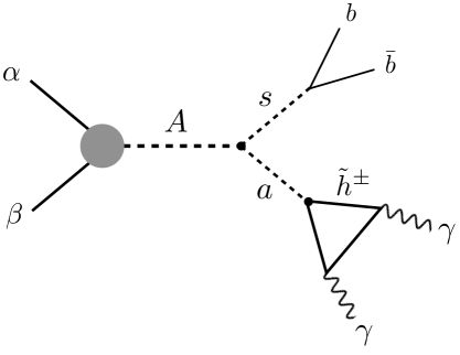
In NMSSM $a\to\gamma\gamma$ is induced by a higgsino loop diagram also shown in Fig. 1. The $Y_{d}=h$ is disfavoured because non-zero $Aha$ coupling requires doublet-singlet mixing in the pseudo-scalar sector ($Aa$ mixing), suppressing $a\to\gamma\gamma$ branching ratio. In our scenario, $s$ predominantly decays into $b\bar{b}$ through a mixing with $H$. Although the current data would not have enough sensitivity to discriminate these extra jets from other jets with QCD origin, this scenario can be tested by looking at these $b$-jets in the future analysis.

The paper is organised as follows. In section 2 we demonstrate our scenario in a simplified framework in which the mixing between singlet and doublet states are ignored. In section 3 we consider how our scenario can be realised in the NMSSM taking the effect of mixing into account. We conclude this paper in section 4.

2 Interpretation with pure states

We first discuss our scenario in a simplified framework where the resonance $A$ is pure doublet state and the lightest CP even and odd Higgs bosons, $s$ and $a$, are exclusively originated from the singlet field $S$. The signal of the diphoton excess is given by

$$(\sigma\cdot{\rm BR})^{\rm signal}\equiv\sigma(pp\to A)\cdot{\rm BR}(A\to sa)\cdot{\rm BR}(a\to\gamma\gamma)$$ (1)

where the cross section $\sigma(pp\to A)$ depends on the centre of mass energy of the proton-proton collision.

Figure 2: Production cross section of $A$ from the $b\bar{b}$ (red) and $gg$ (blue) initial states as a function of $m_{A}$ for $\sqrt{S}=13$ (solid) and 8 (dashed) TeV. In the left (right) panel, the thick and thin lines correspond to $\tan\beta=50$ and 30 (1.5 and 3), respectively. For the $b\bar{b}$ initial state with $\tan\beta=50$, $m_{A}\lesssim 840$ GeV is excluded by the $b\bar{b}\to A\to\tau^{+}\tau^{-}$ search.

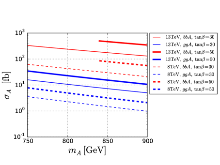
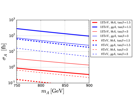
Fig. 2 shows the NLO production cross section of $A$ from the $b\bar{b}$ (red) and $gg$ (blue) initial states as a function of $m_{A}$ for $\sqrt{S}=13$ (solid) and 8 (dashed) TeV. In the left (right) panel of Fig. 2, the thick and thin lines correspond to $\tan\beta=50$ and 30 (1.5 and 3), respectively. The cross sections are calculated using SusHi v.1.5.0 [76, 77, 78, 79, 80, 81, 82, 83]. As can be seen, the $\sqrt{S}=13$ TeV production cross section for large (small) $\tan\beta$ values is dominated by $b\bar{b}$ ($gg$) initial state. It can be as large as 400 (200) fb for $\tan\beta=50$ (30) at $m_{A}\sim 850$ GeV. The cross section enhances from 8 TeV to 13 TeV by factor of 5 for $gg$ and 6.7 for $b\bar{b}$ initial states. We impose the $m_{A}$ dependent upper limit on $\sigma(b\bar{b}\to A)\cdot{\rm BR}(A\to\tau^{+}\tau^{-})$ and $\sigma(gg\to A)\cdot{\rm BR}(A\to\tau^{+}\tau^{-})$ obtained from the 8 TeV CMS search for the neutral Higgs boson decaying to di-tau [84]. We found the $m_{A}\;\raisebox{-3.00003pt}{$\stackrel{{\scriptstyle\displaystyle<}}{{\sim}}$}\;840$ GeV is excluded by this constraint for $b\bar{b}$ initial state at $\tan\beta=50$ and this region is not shown in Fig. 2. For $\tan\beta=30$ or the $gg$ initial state, the whole region with $m_{A}>750$ GeV is allowed.

We define the interaction between $A$-$s$-$a$ as

$${\cal L}\supset g_{Asa}Asa\,.$$ (2)

With the coupling $g_{Asa}$, the partial decay rate of $A\to sa$ is given by

$$\Gamma(A\to sa)=\frac{|g_{Asa}|^{2}}{16\pi m_{A}}\bar{\lambda}(\frac{m_{s}^{2}}{m_{A}^{2}},\frac{m_{a}^{2}}{m_{A}^{2}}),$$ (3)

where $\bar{\lambda}(a,b)\equiv 1+a^{2}+b^{2}-2(a+b+ab)$. In what follows we assume $m_{s}=65$ GeV and $815\leq m_{A}\leq 875$ GeV. In this parameter region, $h\to ss$ and $A\to ha$ are kinematically forbidden while $A\to sa$ is allowed.

The $A\to sa$ decay mode competes with $A\to b\bar{b}$ and $A\to t\bar{t}$ in the large and small $\tan\beta$ regimes, respectively. The partial decay rates are given by

$$\Gamma(A\to b\bar{b})=\frac{3\alpha_{W}m_{A}}{8m_{W}^{2}}m_{b}^{2}\tan^{2}\beta\Big{(}1-\frac{4m_{b}^{2}}{m_{A}^{2}}\Big{)}^{1/2},~{}~{}~{}\Gamma(A\to t\bar{t})=\frac{3\alpha_{W}m_{A}}{8m_{W}^{2}}m_{t}^{2}\cot^{2}\beta\Big{(}1-\frac{4m_{t}^{2}}{m_{A}^{2}}\Big{)}^{1/2}\,.$$ (4)

The decay modes into gauge bosons are highly suppressed due to the CP property. Fig. 3 shows the branching ratio of $A\to sa$ for $m_{A}=850$ GeV, $m_{s}=65$ GeV as a function of $\tan\beta$ and $|g_{Asa}|/(246\,\rm GeV)$.

Figure 3: Branching ratio of $A\to sa$ as a function of $\tan\beta$ and $g_{Asa}/(246\,\rm GeV)$. We fix $m_{A}=850$ GeV and $m_{s}=65$ GeV.

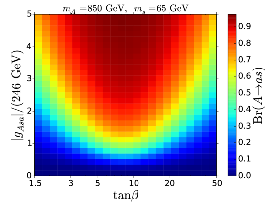
At a fixed $g_{Asa}$, ${\rm BR}(A\to sa)$ is maximised around $\tan\beta\sim 7$. This is because the decay rate of $A\to f\bar{f}$ is minimised in this region. For small ($\;\raisebox{-3.00003pt}{$\stackrel{{\scriptstyle\displaystyle<}}{{\sim}}$}\;2$) and large ($\;\raisebox{-3.00003pt}{$\stackrel{{\scriptstyle\displaystyle>}}{{\sim}}$}\;30$) $\tan\beta$, $|g_{Asa}|/(246\,\rm GeV)\;\raisebox{-3.00003pt}{$\stackrel{{\scriptstyle\displaystyle>}}{{\sim}}$}\;1.5$ is required to have ${\rm BR}(A\to sa)\;\raisebox{-3.00003pt}{$\stackrel{{\scriptstyle\displaystyle>}}{{\sim}}$}\;0.3$.

We focus on the process in which $a$ decays to two photons through higgsino loop. If $a$ is pure singlet and the gauginos are decoupled, ${\rm BR}(a\to\gamma\gamma)$ does not depend on the higgsino mass nor the $a\tilde{h}^{+}\tilde{h}^{-}$ coupling, and is entirely determined by quantum numbers of higgsinos. The branching ratios are given as

$${\rm BR}(a\to W^{+}W^{-})\approx 0.65,~{}~{}~{}~{}{\rm BR}(a\to ZZ)\approx 0.23,~{}~{}~{}~{}{\rm BR}(a\to\gamma Z)\approx 0.05,~{}~{}~{}~{}{\rm BR}(a\to\gamma\gamma)\approx 0.07.$$ (5)

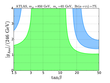
We now combine the cross section and branching ratios to see if the model can fit the 13 TeV excess consistently with the 8 TeV data. Since the CMS detailed data analysis and the fit of ref. [5] to the ATLAS data are not on equal footing, we do not average their results and discuss them in turn. The results for the coupling $g_{Asa}$ based on the CMS analysis are summarized in the left panel of Fig. 4.

Figure 4: Left: The results for the coupling $g_{Asa}$ as a function of $\tan\beta$ based on the CMS fit. The blue (yellow) region is favoured by the 13 TeV excess at 1 $\sigma$ (2 $\sigma$) level. The green region is favoured by the excess in the 8 TeV data at 1 $\sigma$ level. (The blue and green regions partly overlap.) The grey region is beyond the 2-$\sigma$ in the 8 TeV data. Right: The results for the coupling $g_{Asa}$ as a function of $\tan\beta$ based on the fit of ref. [5] to the ATLAS data. The blue region is favoured by the 13 TeV excess at 1 $\sigma$ level. The green region is favoured by the excess in the 8 TeV data at 1 $\sigma$ level.

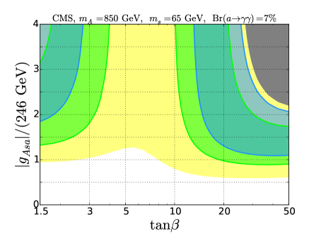
The blue region is favoured by the 13 TeV excess at 1 $\sigma$ level, $(\sigma\cdot{\rm BR})^{\rm signal}_{\rm 13TeV}\in[2.6,\,7.7]\,$ fb, and the yellow one by the 2 $\sigma$ range $[0.85,\,12]$ fb. The green region is favoured by the excess in the 8 TeV data at 1 $\sigma$ level, $(\sigma\cdot{\rm BR})^{\rm signal}_{\rm 8TeV}\in[0.31,\,1.00]$ fb. The grey region corresponds to $(\sigma\cdot{\rm BR})^{\rm signal}_{\rm 8TeV}>1.45~{}{\rm fb}$ which is disfavoured at 2-$\sigma$ at 8 TeV.

As can be seen, there exist two favoured regions, ($a$) small ($\;\raisebox{-3.00003pt}{$\stackrel{{\scriptstyle\displaystyle<}}{{\sim}}$}\;2$) $\tan\beta$ region and ($b$) large ($\;\raisebox{-3.00003pt}{$\stackrel{{\scriptstyle\displaystyle>}}{{\sim}}$}\;20$) $\tan\beta$ region. This is because the production cross section, $pp\to A$, is maximised for these two regions. In the small $\tan\beta$ region $gg\to A$ via the top-quark loop dominates the production processes, whereas $b\bar{b}\to A$ is dominant in the large $\tan\beta$ region. The enhancement in the cross section compensates the slight suppression in ${\rm BR}(A\to sa)$ (see Fig. 3). For moderate $\tan\beta$, the signal event rate cannot be large enough to be within the 1 $\sigma$ regions due to the small cross section even for $|g_{Asa}|/(246\,{\rm GeV})\;\raisebox{-3.00003pt}{$\stackrel{{\scriptstyle\displaystyle>}}{{\sim}}$}\;1.5$ where the ${\rm BR}(A\to sa)$ is already saturated ${\rm BR}(A\to sa)\sim 1$ and increasing $g_{Asa}$ further does not help to enhance the signal rate. As can be seen, both favoured regions require relatively large $g_{Asa}$ coupling. For large and small $\tan\beta$ regions, the 1 $\sigma$ region requires $|g_{Asa}|/(246\,{\rm GeV})\;\raisebox{-3.00003pt}{$\stackrel{{\scriptstyle\displaystyle>}}{{\sim}}$}\;1$ and 2, respectively.

In the right panel of Fig. 4 we show the results for the coupling $g_{Asa}$ based on the fit of ref. [5] to the ATLAS data. We see that the tension between the 13 and 8 TeV data does not disappear even with the cascade decay topology, where the primary object has the mass of 850 GeV, and remains at the level of approximately 2 $\sigma$. The excess at 13 TeV requires, at 1 $\sigma$, somewhat larger values of the coupling $g_{Asa}$.

In the simplified framework discussed so far, the dominant decay mode of $s$ becomes $s\to\gamma\gamma$ because other gauge boson final states are not kinematically allowed. This will cause a strong tension with the fact that ATLAS and CMS did not observe extra photons other than the diphoton excess with $m_{\gamma\gamma}\simeq 750$ GeV. However, this problem can be easily circumvented by introducing a mixing between $s$ and $H$. With this mixing $s$ will dominantly decay into $b\bar{b}$.

3 Realisation in NMSSM

The superpotential and soft SUSY breaking Lagrangian of the NMSSM are given by (c.f. [86])

$$W=W_{\rm MSSM}+\lambda SH_{u}H_{d}+\xi_{F}S+\frac{1}{2}\mu^{\prime}S^{2}+\frac{\kappa}{3}S^{3}\,,$$ (6)

$$-{\cal L}_{\rm soft}=-{\cal L}_{\rm soft}^{\rm MSSM}+m_{S}^{2}|S|^{2}+\Big{[}\lambda A_{\lambda}SH_{u}H_{d}+\frac{1}{3}\kappa A_{\kappa}S^{3}+\frac{1}{2}m^{\prime 2}_{3}S^{2}+\xi_{S}S+{\rm h.c.}\Big{]}\,,$$ (7)

where we assume all couplings are real. Notice that the MSSM $\mu$-term, $W_{\rm MSSM}\supset\mu_{\rm MSSM}H_{u}H_{d}$, can be removed by redefining $S$ by a constant shift. We fix $S$ in this way, hence $\mu_{\rm MSSM}=0$. We first rotate the doublet Higgs bosons $H_{u}$ and $H_{d}$ by the angle $\beta$ and define the new field basis

$$\hat{H}=\sin\beta H_{dR}^{0}-\cos\beta H_{uR}^{0}\,,~{}~{}\hat{h}=\cos\beta H_{dR}^{0}+\sin\beta H_{uR}^{0}\,,~{}~{}\hat{s}=S_{R}\,,$$ (8)

$$\hat{A}=\sin\beta H_{dI}^{0}+\cos\beta H_{uI}^{0}\,,~{}~{}~{}\hat{G}=\cos\beta H_{dI}^{0}-\sin\beta H_{uI}^{0}\,,~{}~{}~{}\hat{a}=S_{I}\,.$$ (9)

By this rotation, $\hat{H}$ does not have the vacuum expectation value, and $\hat{G}$ becomes the Goldstone boson eaten by $Z$. The scalar mass eigenstates, denoted by $h_{i}$ (with $h_{i}=h,H,s$ where $h$ is the SM-like Higgs), are expressed in terms of the hatted fields with the help of the diagonalization matrix $\tilde{S}$:

$$h_{i}=\tilde{S}_{h_{i}\hat{h}}\hat{h}+\tilde{S}_{h_{i}\hat{H}}\hat{H}+\tilde{S}_{h_{i}\hat{s}}\hat{s}\,.$$ (10)

The pseudoscalar mass eigenstates, $A$ and $a$, are related to the hatted fields, $\hat{A}$ and $\hat{a}$, by a rotation by angle $\theta_{Aa}$.

The $\hat{A}$-$\hat{s}$-$\hat{a}$ interaction is given by the F-term of $S$ as $|\frac{\partial W}{\partial S}|^{2}\supset\lambda\kappa H_{u}H_{d}S^{*}S^{*}\supset-v_{\rm SM}\lambda\kappa\hat{A}\hat{s}\hat{a}$, where $v_{\rm SM}=246$ GeV. In the previous section we mentioned that one should allow the $\hat{H}$-$\hat{s}$ mixing in order to suppress unwanted $s\to\gamma\gamma$ decay. Neglecting $A$-$a$ mixing, the coupling $g_{Asa}$ is given as

$$g_{Asa}/v_{\rm SM}=-\lambda\kappa\tilde{S}_{s\hat{s}}\,.$$ (11)

In the previous section we have shown that $|g_{Asa}/v_{\rm SM}|\;\raisebox{-3.00003pt}{$\stackrel{{\scriptstyle\displaystyle>}}{{\sim}}$}\;1$ (2) is required for $\tan\beta\;\raisebox{-3.00003pt}{$\stackrel{{\scriptstyle\displaystyle>}}{{\sim}}$}\;20$ ($\;\raisebox{-3.00003pt}{$\stackrel{{\scriptstyle\displaystyle<}}{{\sim}}$}\;2$) (See Fig. 4.). Clearly, one needs the product $|\lambda\kappa|\;\raisebox{-3.00003pt}{$\stackrel{{\scriptstyle\displaystyle>}}{{\sim}}$}\;1$ (2) for large (small) $\tan\beta$ to explain the excess. Such large values of $\lambda$ and/or $\kappa$ indicate the Landau pole at the scale $\mu_{\rm UV}$ much below the GUT scale. In Fig. 5 we show the constraint from the Landau pole.

Figure 5: The limit for the Landau pole constraint. At the green (blue and red) contour ${\rm max}[\lambda(\mu_{\rm UV}),\kappa(\mu_{\rm UV})]=5$, where $\mu_{\rm UV}=500\mu$, ($100\mu$, $50\mu$).

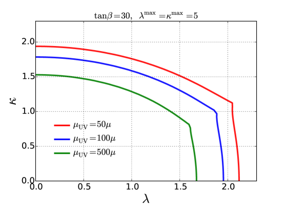
If our topology is responsible for the observed diphoton excess, this indicates the existence of the UV cut-off typically of the order of 100 TeV.

Dropping the Goldstone mode, the entries of the mass matrix for the pseudo-scalar sector $(A,a)$ are given by

$$M^{2}_{\hat{A}\hat{A}} = \frac{2(\mu B_{\rm eff}+\hat{m}_{3}^{2})}{\sin 2\beta}+\Delta^{2}_{AA},$$ (12)

$$M^{2}_{\hat{a}\hat{a}} = \frac{1}{v_{s}}\left[\frac{\lambda v_{\rm SM}^{2}\sin 2\beta}{4}(B_{\rm eff}+\mu^{\prime})-\xi_{F}\mu^{\prime}-\xi_{S}\right]$$ (13)

$$+\kappa\left[\frac{3\lambda v_{\rm SM}^{2}\sin 2\beta}{4}-4\xi_{F}\right]-2m^{\prime 2}_{S}-\kappa v_{s}(3A_{\kappa}+\mu^{\prime})+\Delta^{2}_{aa},$$

$$M^{2}_{\hat{A}\hat{a}} = \frac{\lambda v_{\rm SM}}{\sqrt{2}}(A_{\lambda}-2\kappa v_{s}-\mu^{\prime})+\Delta^{2}_{Aa}\,,$$ (14)

where $B_{\rm eff}\equiv A_{\lambda}+\kappa v_{s}$ and $\hat{m}_{3}^{2}\equiv m_{3}^{2}+\lambda(\mu^{\prime}v_{s}+\xi_{F})$. The $m_{3}^{2}$ is the soft breaking mass term ${\cal L}_{\rm soft}^{\rm MSSM}\supset m_{3}^{2}H_{u}H_{d}$, $v_{s}\equiv\langle s\rangle\equiv\mu/\lambda$ and $\Delta^{2}_{AA/aa/Aa}$ are the radiative corrections.

The mixing between $A$ and $a$ is determined by

$$\sin 2\theta_{Aa}=\frac{2M^{2}_{\hat{A}\hat{a}}}{m_{A}^{2}-m_{a}^{2}}\simeq\frac{\lambda(A_{\lambda}-2\kappa v_{s}-\mu^{\prime})}{460\,{\rm GeV}}+\frac{\Delta^{2}_{Aa}}{(283\,{\rm GeV})^{2}}\,,$$ (15)

where we used $m_{A}=850$ GeV, $m_{a}=750$ GeV. This mixing strongly affects the ${\rm BR}(a\to\gamma\gamma)$ because it introduces $a\to b\bar{b}$ and $t\bar{t}$ modes through the mixing. The reduction of the signal strength can be parameterized by $r$ as

$$(\sigma\cdot{\rm BR})^{\rm signal}=r\cdot(\sigma\cdot{\rm BR})^{\rm signal}_{\rm pure}\,.$$ (16)

For $|\sin\theta_{Aa}|\ll 1$, $r$ can be written as

$$r=\frac{\cos^{2}\theta_{Aa}\Gamma^{a}_{VV}}{\sin^{2}\theta_{Aa}\Gamma^{A}_{f\bar{f}}+\cos^{2}\theta_{Aa}\Gamma^{a}_{VV}}$$ (17)

where $\Gamma^{A}_{f\bar{f}}$ is the sum of the partial decay rates in Eq. (4) at $m_{A}=750$ GeV and $\Gamma^{a}_{VV}$ is the sum of the partial decay rates of the pure state $a$ into $W^{+}W^{-}$, $ZZ$, $Z\gamma$ and $\gamma\gamma$, which can be written as

$$\Gamma^{a}_{VV}=|\lambda|^{2}f(m_{\tilde{h}})\,.$$ (18)

The factor $|\lambda|^{2}$ can be understood because $a\tilde{h}\tilde{h}$ coupling is given by $\frac{\lambda}{\sqrt{2}}$. The $f(m_{\tilde{h}})$ is obtained from the higgsino loop diagram and we find $f(m_{\tilde{h}})\simeq 1.5\cdot 10^{-2}$ GeV for $m_{\tilde{h}}=|\mu|\simeq 375$ GeV. The condition $r\;\raisebox{-3.00003pt}{$\stackrel{{\scriptstyle\displaystyle>}}{{\sim}}$}\;0.5$ can be translated as

$$|\tan\theta_{Aa}|\;\raisebox{-3.00003pt}{$\stackrel{{\scriptstyle\displaystyle<}}{{\sim}}$}\;\Big{[}\frac{|\lambda|^{2}f(m_{\tilde{h}})}{\Gamma^{A}_{f\bar{f}}}\Big{]}^{1/2}\sim 0.03\,|\lambda|$$ (19)

for large ($\;\raisebox{-3.00003pt}{$\stackrel{{\scriptstyle\displaystyle>}}{{\sim}}$}\;10$) or small ($\;\raisebox{-3.00003pt}{$\stackrel{{\scriptstyle\displaystyle<}}{{\sim}}$}\;2$) $\tan\beta$. This puts a strong constraint on the parameters appearing in Eq. (15).

In the scalar sector ($\hat{H}$, $\hat{h}$, $\hat{s}$), the elements of the mass matrix are given by

$$M^{2}_{\hat{H}\hat{H}} = M^{2}_{AA}+(m_{Z}^{2}-\frac{\lambda^{2}}{2}v_{\rm SM}^{2})\sin^{2}2\beta+\Delta^{2}_{HH},$$ (20)

$$M^{2}_{\hat{h}\hat{h}} = m_{Z}^{2}\cos^{2}2\beta+\frac{\lambda^{2}}{2}v_{\rm SM}^{2}\sin^{2}2\beta+(\delta m_{h}^{2})^{\rm rad}+\Delta^{2}_{hh},$$ (21)

$$M^{2}_{\hat{s}\hat{s}} = \kappa v_{s}(4\kappa v_{s}+A_{\kappa}+3\mu^{\prime})+\frac{1}{v_{s}}\Big{[}\frac{\lambda v_{\rm SM}^{2}\sin 2\beta}{4}(A_{\lambda}+\mu^{\prime})-(\mu^{\prime}\xi_{F}+\xi_{S})\Big{]}+\Delta^{2}_{ss},$$ (22)

$$M^{2}_{\hat{H}\hat{h}} = \frac{1}{2}(m_{Z}^{2}-\frac{\lambda^{2}}{2}v_{\rm SM}^{2})\sin 4\beta+\Delta^{2}_{Hh},$$ (23)

$$M^{2}_{\hat{H}\hat{s}} = \frac{\lambda}{\sqrt{2}}v_{\rm SM}\Lambda\cos 2\beta+\Delta^{2}_{Hs},$$ (24)

$$M^{2}_{\hat{h}\hat{s}} = \frac{\lambda}{\sqrt{2}}v_{\rm SM}(2\mu-\Lambda\sin 2\beta)+\Delta^{2}_{hs}\,,$$ (25)

where $\Lambda\equiv B_{\rm eff}+\kappa v_{s}+\mu^{\prime}=A_{\lambda}+2\kappa v_{s}+\mu^{\prime}$ and $(\delta m_{h}^{2})^{\rm rad}$ is the radiative correction induced by the stop loop. Typically, for large $\tan\beta$ this scenario requires heavy stops ($m_{\tilde{t}}\sim{\cal O}(10)$ TeV) depending on the size of the stop mixing parameter $X_{t}$ in order to achieve $m_{h}=125$ GeV. The $\Delta^{2}_{HH/hh/ss/Hh/Hs/hs}$ are the radiative corrections contributing to the NMSSM Higgs boson mass matrices.

The elements of the diagonalization matrix $\tilde{S}$ must respect various phenomenological constraints. The LEP limit on the $e^{+}e^{-}\to Z^{*}\to Zs$ $(s\to b\bar{b})$ process for the 65 GeV scalar gives the bound $\tilde{S}_{s\hat{h}}\cdot{\rm BR}(s\to b\bar{b})\;\raisebox{-3.00003pt}{$\stackrel{{\scriptstyle\displaystyle<}}{{\sim}}$}\;0.16$ [89], where ${\rm BR}(s\to b\bar{b})$ depends in principle on $\tilde{S}_{s\hat{H}}$ mixing and $\tan\beta$ [90]. The measurements of the properties of the SM-like Higgs boson at the LHC also give constraints on the mixing angles. The deviation of its coupling to the gauge bosons is now constrained up to $\sim 20$ % at 95 % CL [91, 92]. This translates into the constraint on the $\tilde{S}$ entries as $\tilde{S}_{h\hat{H}},\tilde{S}_{h\hat{s}}\;\raisebox{-3.00003pt}{$\stackrel{{\scriptstyle\displaystyle<}}{{\sim}}$}\;0.2$.

In the parameter space relevant for our model, the elements $\tilde{S}_{s\hat{H}}$ and $\tilde{S}_{H\hat{s}}$ remain unconstrained and may be large. Neglecting the small mixing elements they may be approximated by

$$\tilde{S}_{s\hat{H}}\simeq\sin\theta_{sH}\simeq-\tilde{S}_{H\hat{s}}\,,$$ (26)

where for future convenience we introduced the mixing angle $\theta_{sH}$ satisfying

$$\sin 2\theta_{sH}=\frac{2M^{2}_{Hs}}{m_{s}^{2}-m_{H}^{2}}\simeq-\frac{\lambda\Lambda\cos 2\beta}{2\,{\rm TeV}}-\frac{\Delta^{2}_{Hs}}{(600\,{\rm GeV})^{2}}\,,$$ (27)

In the last equality we have used $m_{H}=850$ GeV, $m_{s}=65$ GeV. The two small off-diagonal entries of $\tilde{S}$ may be approximated as follows

$$\tilde{S}_{s\hat{h}}\simeq\frac{\cos\theta_{sH}M^{2}_{\hat{h}\hat{s}}+\sin\theta_{sH}M^{2}_{\hat{H}\hat{h}}}{m_{s}^{2}-m_{h}^{2}}\,,\qquad\tilde{S}_{H\hat{h}}\simeq\frac{\cos\theta_{sH}M^{2}_{\hat{H}\hat{h}}-\sin\theta_{sH}M^{2}_{\hat{h}\hat{s}}}{m_{H}^{2}-m_{h}^{2}}\,.$$ (28)

The elements $\tilde{S}_{h\hat{H}}$ and $\tilde{S}_{h\hat{s}}$ are related to the above ones by orthogonality of $\tilde{S}$:

$$\tilde{S}_{h\hat{s}}\simeq-\cos\theta_{sH}\tilde{S}_{s\hat{h}}+\sin\theta_{sH}\tilde{S}_{H\hat{h}}\,,\qquad\tilde{S}_{h\hat{H}}\simeq-\cos\theta_{sH}\tilde{S}_{H\hat{h}}-\sin\theta_{sH}\tilde{S}_{s\hat{h}}\,.$$ (29)

Clearly, the values of the Higgs boson masses and the constraints on the mixing angles would select some regions of the NMSSM parameter space. However, the complexity of the NMSSM Higgs potential make a full quantitative analysis of our scenario, with radiative corrections included, challenging and premature. Merely for the illustration purpose, we attempt to find the NMSSM parameters that satisfy the above conditions using approximate forms of the 1-loop radiative corrections. Some attention has to be paid to the magnitude of the radiative corrections. Indeed, we note that some of the 1-loop radiative correction terms are proportional to the 3rd power of $\lambda$ or $\kappa$ and can be as large as the tree level terms for $|\lambda|$, $|\kappa|\;\raisebox{-3.00003pt}{$\stackrel{{\scriptstyle\displaystyle>}}{{\sim}}$}\;1$ [93]. The 2-loop corrections may also be large [94] in this region. For large $\lambda$ and $\kappa$, neglecting the corrections proportional to the gauge and Yukawa couplings, the leading terms of the radiative corrections to the off-diagonal mass matrix elements are given by

$$\Delta^{2}_{Hs} = \frac{\kappa v_{\rm SM}\mu}{8\sqrt{2}\pi^{2}}\,\left(2\lambda^{2}L_{\mu}+2\kappa^{2}L_{\nu}-3\lambda^{2}L_{\mu\nu}\right)\cos(2\beta)\,,$$ (30)

$$\Delta^{2}_{hs} = \frac{\lambda v_{\rm SM}\mu}{8\sqrt{2}\pi^{2}}\,\left(2\lambda^{2}L_{\mu}+2\kappa^{2}L_{\nu}-\left(\lambda^{2}+8\kappa^{2}\right)L_{\mu\nu}\right)-\Delta^{2}_{Hs}\tan(2\beta)\,,$$ (31)

$$\Delta^{2}_{Aa} = \Delta^{2}_{Hh}\,\,=\,\,0\,,$$ (32)

where

$$L_{\mu}=\ln\left(\frac{\mu^{2}}{M_{Z}^{2}}\right),\qquad L_{\nu}=\ln\left(\frac{(2\kappa v_{s}+\mu^{\prime})^{2}}{M_{Z}^{2}}\right),\qquad L_{\mu\nu}=\ln\left(\frac{\max(\mu^{2},(2\kappa v_{s}+\mu^{\prime})^{2})}{M_{Z}^{2}}\right).$$ (33)

It is easy to find solutions for the parameters of the model satisfying the constraints $m_{H}=m_{A}=850$ GeV, $m_{s}=65$ GeV , $\mu=375$ GeV, vanishing $Aa$ mixing ($\theta_{Aa}=0$) and small $\tilde{S}_{s\hat{h}}$. We used the following procedure: The scalar mass squared matrix has 6 independent parameters. We choose them as 3 eigenvalues ($m_{h}^{2}$, $m_{H}^{2}$, $m_{s}^{2}$) and 3 off-diagonal entries of the diagonalization matrix ($\tilde{S}_{s\hat{H}}$, $\tilde{S}_{s\hat{h}}$, $\tilde{S}_{h\hat{H}}$). Using this parameterization we calculate the off-diagonal elements of the scalar mass squared matrix and compare them with the same elements expressed by the parameters of the model in eqs. (23)-(25). One of the parameters, $\mu^{\prime}$, is fixed by the requirement of vanishing $A$-$a$ mixing: $\mu^{\prime}=A_{\lambda}-2\mu\kappa/\lambda$. Then, for some fixed values of the elements ($\tilde{S}_{s\hat{H}}$, $\tilde{S}_{s\hat{h}}$, $\tilde{S}_{h\hat{H}}$), we are left with the set of three equations for three parameters: $\lambda$, $\kappa$ and $A_{\lambda}$. In general there is a discrete set of solutions.

Figure 6: Left panel: $\lambda$ (solid) and $|\kappa|$ (dashed) as functions of $\tilde{S}_{s\hat{H}}$. Right panel: the SM-like Higgs boson mass at the tree level, $m_{h}^{\rm tree}$, (dashed) and with the leading (for large $\lambda$ and $\kappa$) loop corrections (but before including the radiative correction from the scalar top loop), $\widetilde{m}_{h}$, (solid) as functions of $\tilde{S}_{s\hat{H}}$. Solutions with positive (red) and negative (blue) values of $\kappa$ are shown. Other parameters are fixed at: $\tan\beta=20$, $|g_{Asa}|=0.6$, $\tilde{S}_{s\hat{h}}=0$.

In the actual numerical calculations we had to modify this simple prescription. In order to compare our results with the experimental constraints illustrated in Fig. 4 we were fixing the value of $g_{Asa}$ given by eq. (11). This fixes one combination of the parameters $\lambda$, $\kappa$ and $A_{\lambda}$. Thus, only two mixing elements (chosen to be $\tilde{S}_{s\hat{H}}$, $\tilde{S}_{s\hat{h}}$) remain as input for our calculations while the third one ($\tilde{S}_{h\hat{H}}$) is obtained as output. Numerical iteration procedures are used to find solutions.

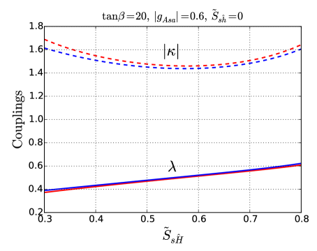
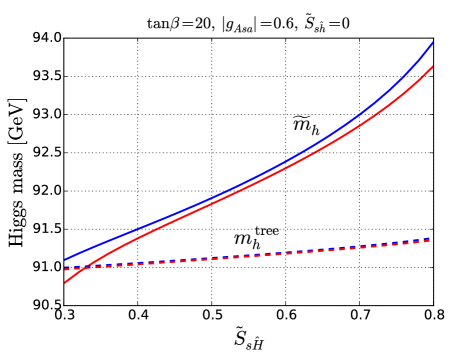
One of the input mixing elements, $\tilde{S}_{s\hat{h}}$, is quite strongly constrained by the LEP data. Thus, after fixing the values of the scalar masses and $\tan\beta$, $\tilde{S}_{s\hat{H}}$ remains the only input quantity which may be changed in a relatively wide range. The dependence of the results on $\tilde{S}_{s\hat{H}}$ is shown in Fig. 6 for the example with $\tan\beta=20$, $\tilde{S}_{s\hat{h}}=0$ and $|g_{Asa}|=0.6$. One can see that $\lambda$ increases with $\tilde{S}_{s\hat{H}}$ while $|\kappa|$ has a minimum. The behavior of $\lambda$ follows from the fact that for bigger mixing $\tilde{S}_{s\hat{H}}$ one needs bigger $M^{2}_{\hat{H}\hat{s}}$ which grows with $\lambda$ (at least the tree contribution, see eq. (24)). Then the behavior of $\kappa$ follows from relation (11). The leading (in $\lambda$ and $\kappa$) loop correction to the Higgs mass is a quite complicated function of the parameters. From the right panel in Fig. 6 one can see that it may even vanish for some combination of $\lambda$ and $\kappa$ but generally is an increasing function of the input mixing parameter $\tilde{S}_{s\hat{H}}$. Examples presented in Fig. 6 (and in Table 1) were obtained for $\tilde{S}_{s\hat{h}}=0$. We checked that the results do not change substantially for the values of $\tilde{S}_{s\hat{h}}$ allowed by the LEP data.

A few generic examples are presented in Table 1. For large $\tan\beta$ the values of $\tilde{S}_{s\hat{H}}$ are chosen to give $|\kappa|$ close to the smallest possible (for a given set of other parameters) value in order to get the Landau pole scale as big as possible. For small $\tan\beta$ we have to choose much smaller $\tilde{S}_{s\hat{H}}$ in order to avoid huge tree level contribution to the Higgs mass (value of $\lambda$ increases with $\tilde{S}_{s\hat{H}}$). The first example in Table 1 shows that $\tilde{S}_{s\hat{H}}\;\raisebox{-3.00003pt}{$\stackrel{{\scriptstyle\displaystyle>}}{{\sim}}$}\;0.1$ can easily lead to too large $m_{h}^{\rm tree}$ for $\tan\beta=2$. The last two columns of Table 1 show the SM-like Higgs boson at the tree level, $m_{h}^{\rm tree}$, and with the leading (for large $\lambda$ and $\kappa$) loop corrections, $\widetilde{m}_{h}$ (but before including the radiative correction from the scalar top loop). An interesting observation is that in the parameter range selected by the constraints of very small $\hat{h}$-$\hat{s}$ and $\hat{A}$-$\hat{a}$ mixings the radiative corrections to the Higgs potential from the NMSSM Higgs bosons are actually small, in spite of the sizable values of $\lambda$ and, particularly, $\kappa$. This is related to the fact that some of potentially large contributions are proportional to appropriate mixing elements and are small in the limit of small mixings. Thus, the values of $\widetilde{m}_{h}$ given in Table 1 are almost entirely controlled by the tree-level effects. The mixing elements, other than $\tilde{S}_{s\hat{H}}\approx-\tilde{S}_{H\hat{s}}$, are small once $\tilde{S}_{s\hat{h}}$ is taken to be small (to fulfill the LEP constrains). $\tilde{S}_{H\hat{h}}$ is suppressed by $m_{H}^{2}$ (see eqs. (28)) and typically is below 0.01. The two remaining off-diagonal elements are also small due to relations (29). $\tilde{S}_{h\hat{s}}\approx-\tilde{S}_{s\hat{h}}$ up to small corrections while $|\tilde{S}_{h\hat{H}}|<0.1$ ($<0.01$ in most cases). All these mixing elements are well below present experimental bounds. The numbers given in the table illustrate the expected order of magnitude for the soft mass parameters necessary to explain the di-photon excess in our scenario and indicate that it will be fine-tuned at the level of 1 per mille.

$\tan\beta$	$|g_{Asa}|$	$\tilde{S}_{s\hat{H}}$	$\lambda$	$\kappa$	$A_{\lambda}$ [TeV]	$\mu^{\prime}$ [TeV]	$m_{h}^{\rm tree}$ [GeV]	$\widetilde{m}_{h}$ [GeV]
2	2.1	0.15	1.38	$-$1.54	0.39	1.23	199	215
2	1.4	0.05	0.69	$-$2.04	0.41	2.63	110	112
2	1.0	0.09	0.79	$-$1.27	0.42	1.62	123	125
2	1.0	0.06	0.62	1.61	0.27	1.68	102	113
7	1.4	0.4	0.97	$-$1.57	0.87	2.07	100	112
20	1.3	0.5	0.80	$-$1.88	1.29	3.05	92	96
20	1.0	0.6	0.70	1.78	1.25	$-$0.65	92	95
20	0.6	0.6	0.51	1.46	1.79	$-$0.35	91	92

Table 1: Examples of solutions with vanishing $\tilde{S}_{s\hat{h}}$ and $\theta_{Aa}$ for $m_{H}=m_{A}=850$ GeV, $m_{s}=65$ GeV and $\mu=375$ GeV. The SM-like Higgs boson mass at the tree level, $m_{h}^{\rm tree}$, and with the leading (for large $\lambda$ and $\kappa$) loop corrections (but before including the radiative correction from the scalar top loop), $\widetilde{m}_{h}$, are given in the last two columns. Mixing elements $\tilde{S}_{h\hat{s}}$, $\tilde{S}_{h\hat{H}}$ and $\tilde{S}_{H\hat{h}}$ are at most of order 0.01 for all these examples.

Finally we comment on the constraint from electroweak precision tests. It has been pointed out [95, 96, 97] that large values of $\lambda$ and $\tan\beta$ may introduce a dangerous contribution from light higgsinos to the $T$-parameter [98] as a consequence of violation of SU(2) custodial symmetry. However, generically, in the selected region, $\lambda<1$. Moreover, ref. [95] shows that even for $\lambda=2$ there are strips around the singlino mass parameter $|\mu_{s}|=|\mu^{\prime}+(\kappa/\lambda)\mu|\simeq 750\div 800$ GeV where the higgsino contribution to the $T$-parameter vanishes or is negative independently of $\tan\beta$ and weakly dependent on the value of $\mu$. It is not difficult to find solutions with the singlino mass in the above range, as for instance the last example in Table 1. We, therefore, expect the higgsino contribution to the $T$ parameter not to be a problem for our scenario. One can also expect some cancellation between the higgsino contribution and the contributions from NMSSM Higgs bosons. We leave a detailed numerical analysis for future work.

4 Conclusions

We demonstrate that the plain NMSSM can explain the observed diphoton excess at $m_{\gamma\gamma}\simeq 750$ GeV as a decay of a single particle into two photons at the price of a relatively low UV cut-off (around 100 TeV) and of a certain fine tuning of the parameters. The mechanism behind this scenario is production of a doublet-like pseudo scalar $A$, decaying into a singlet-like pseudo scalar $a$, which subsequently decays via the vector-like higgsino loop into two photons. The predicted width of $a$ is very small, much below the experimental resolution. The two-photon signal should be associated with $b$-quark jets coming from the decay $A\rightarrow as$, with $s$ decaying dominantly into a pair of $b$ quarks. The pseudo scalar $a$ decays also into other channels with the branching ratios given by Eq. (5).

The topology proposed in this paper is the only one that can explain the 750 GeV excess in the plain NMSSM due to a single particle decay. Another possibility for the NMSSM, recently proposed, is to explain the observed signal by the decays of two light pseudo scalars, to two collimated photons each. The latter interpretation could explain a broad peak at 750 GeV, if confirmed experimentally. The width of the signal will give a crucial discrimination between different proposed interpretations, in particular between perturbative and non-perturbative scenarios.

Acknowledgments We thank Michael Schmidt, Kai Schmidt-Hoberg and Florian Staub for valuable comments. MO and SP have been supported by the National Science Centre, Poland, under research grants DEC-2014/15/B/ST2/02157, DEC-2012/04/A/ST2/00099 and DEC-2015/18/M/ST2/00054. MB was supported in part by the Director, Office of Science, Office of High Energy and Nuclear Physics, of the US Department of Energy under Contract DE-AC02-05CH11231 and by the National Science Foundation under grant PHY-1316783. MB acknowledges support from the Polish Ministry of Science and Higher Education (decision no. 1266/MOB/IV/2015/0). SP and KS thank CERN Theory Division for its hospitality during the final work on this project.