Millimeter Wave MIMO Channel Estimation using Overlapped Beam Patterns and Rate Adaptation

Matthew Kokshoorn, Graduate Student Member, IEEE, He Chen, Member, IEEE, Peng Wang, Member, IEEE, Yonghui Li, Senior Member, IEEE, and Branka Vucetic, Fellow, IEEE The material in this paper was presented in part at the IEEE International Conference on Communications, London, England, June 2015 [1] and will be presented in part at IEEE Global Communication Conference, Washington D.C., United States, December 2016 [2]. This research was supported by an Australian Postgraduate Award (APA) and ARC grants DP150104019 and FT120100487. The research was also supported by funding from the Faculty of Engineering and Information Technologies, The University of Sydney, under the Faculty Research Cluster Program and the Faculty Early Career Researcher Scheme. M. Kokshoorn, H. Chen, Y. Li, and B. Vucetic are with School of Electrical and Information Engineering, The University of Sydney, Sydney, NSW 2006, Australia (email: {matthew.kokshoorn, he.chen, yonghui.li, branka.vucetic}@sydney.edu.au). P. Wang was with the School of Electrical and Information Engineering, The University of Sydney, Sydney, NSW 2006, Australia. He is now with Huawei Technologies Sweden AB, Kista 164 40, Sweden (email: wp_ady@hotmail.com).
Abstract

This paper is concerned with the channel estimation problem in Millimeter wave (mmWave) wireless systems with large antenna arrays. By exploiting the inherent sparse nature of the mmWave channel, we first propose a fast channel estimation (FCE) algorithm based on a novel overlapped beam pattern design, which can increase the amount of information carried by each channel measurement and thus reduce the required channel estimation time compared to the existing non-overlapped designs. We develop a maximum likelihood (ML) estimator to optimally extract the path information from the channel measurements. Then, we propose a novel rate-adaptive channel estimation (RACE) algorithm, which can dynamically adjust the number of channel measurements based on the expected probability of estimation error (PEE). The performance of both proposed algorithms is analyzed. For the FCE algorithm, an approximate closed-form expression for the PEE is derived. For the RACE algorithm, a lower bound for the minimum signal energy-to-noise ratio required for a given number of channel measurements is developed based on the Shannon-Hartley theorem. Simulation results show that the FCE algorithm significantly reduces the number of channel estimation measurements compared to the existing algorithms using non-overlapped beam patterns. By adopting the RACE algorithm, we can achieve up to a 6dB gain in signal energy-to-noise ratio for the same PEE compared to the existing algorithms.

I Introduction

Millimeter wave (mmWave) communication has been shown to be a promising technique for next generation wireless systems due to a large expanse of available spectrum [3, 4, 5, 6]. This spectrum, ranging from 30GHz to 300GHz, offers a potential 200 times the bandwidth currently allocated in today’s mobile systems [7]. However, a critical challenge in exploiting the mmWave frequency band is its severe signal propagation loss compared to that over conventional microwave frequencies [5, 8, 9]. To compensate for such a loss, large antenna arrays can be employed to achieve a high power gain. Fortunately, owing to the small wavelength of mmWave signals, these arrays can be packed into small areas at the transmitter and receiver [10, 11]. For such mmWave systems, channel state information (CSI) is essential for effective communication and precoder design. However, the use of large antenna arrays results in a large multiple-input multiple-output (MIMO) channel matrix. This makes the channel estimation of mmWave systems very challenging due to the large number of channel parameters to be estimated. Moreover, owing to the high frequency, it is often not feasible to obtain digital samples from each antenna [3]. To resolve this high frequency sampling problem, analog beamforming techniques have been proposed and widely adopted in open literature (see [12, 13, 14, 10] and references therein). The main idea of analog beamforming is to control the phase of the signal transmitted or received by each antenna via a network of analog phase shifters.

Using analog beamforming techniques, the most straightforward channel estimation method is to exhaustively search in all possible angular directions. Specifically, consider a system with N𝑁N transmit antennas and N𝑁N receive antennas. If we aim at achieving a minimum angular resolution of π/N𝜋𝑁\pi/N, an exhaustive search-based channel estimation would then require a set of N𝑁N transmit beamforming vectors at the transmitter designed to span all possible beam directions and likewise with N𝑁N receive beamforming vectors at the receiver. By searching all possible N2superscript𝑁2N^{2} combinations, an N×N𝑁𝑁N\times N matrix can be formed whose entries represent the channel gains between the N𝑁N transmit and the N𝑁N receive beams. This matrix is commonly referred to as the virtual channel matrix [15, 16, 17, 18, 19]. Despite the large number of entries expected for the mmWave MIMO channel matrix, it has been shown in recent measurements [20, 21] that the mmWave channel exhibits sparse propagation characteristics in the angular domain. That is, there are only a few dominant propagation paths in mmWave channels. This sparsity can be seen in the virtual channel matrix, as only a limited number of transmit and receive direction combinations have a non-zero gain [15]. Therefore, the key objective of mmWave channel estimation is to identify these paths so that the transceiver can align the transmit and receive beams along these paths.

Recently, some compressed sensing based channel estimation algorithms have been proposed to explore the channel sparsity in mmWave systems, e.g., [1, 5, 10, 22]. The fundamental idea in some of these approaches is to search multiple transmit/receive directions in each measurement, by creating initial beam patterns that span a wider angular range than those used by the exhaustive search. Similar adaptive beamforming algorithms and multi-stage codebooks were proposed in [23, 14, 24, 25]. More recent work [26] has also shown that such hierarchical codebooks can be achieved with a single RF chain by exploiting sub-array and deactivation (turning-off) antenna processing techniques. By initially using wider beam patterns, multi-stage approaches are able to reduce the number of measurements required for channel estimation. However, this introduces a loss of directionality gain, leading to a lower signal-to-noise ratio (SNR) at the receiver and a higher probability of estimation error (PEE). In this sense, there exists a challenging trade-off between estimation time and accuracy for mmWave channel estimation.

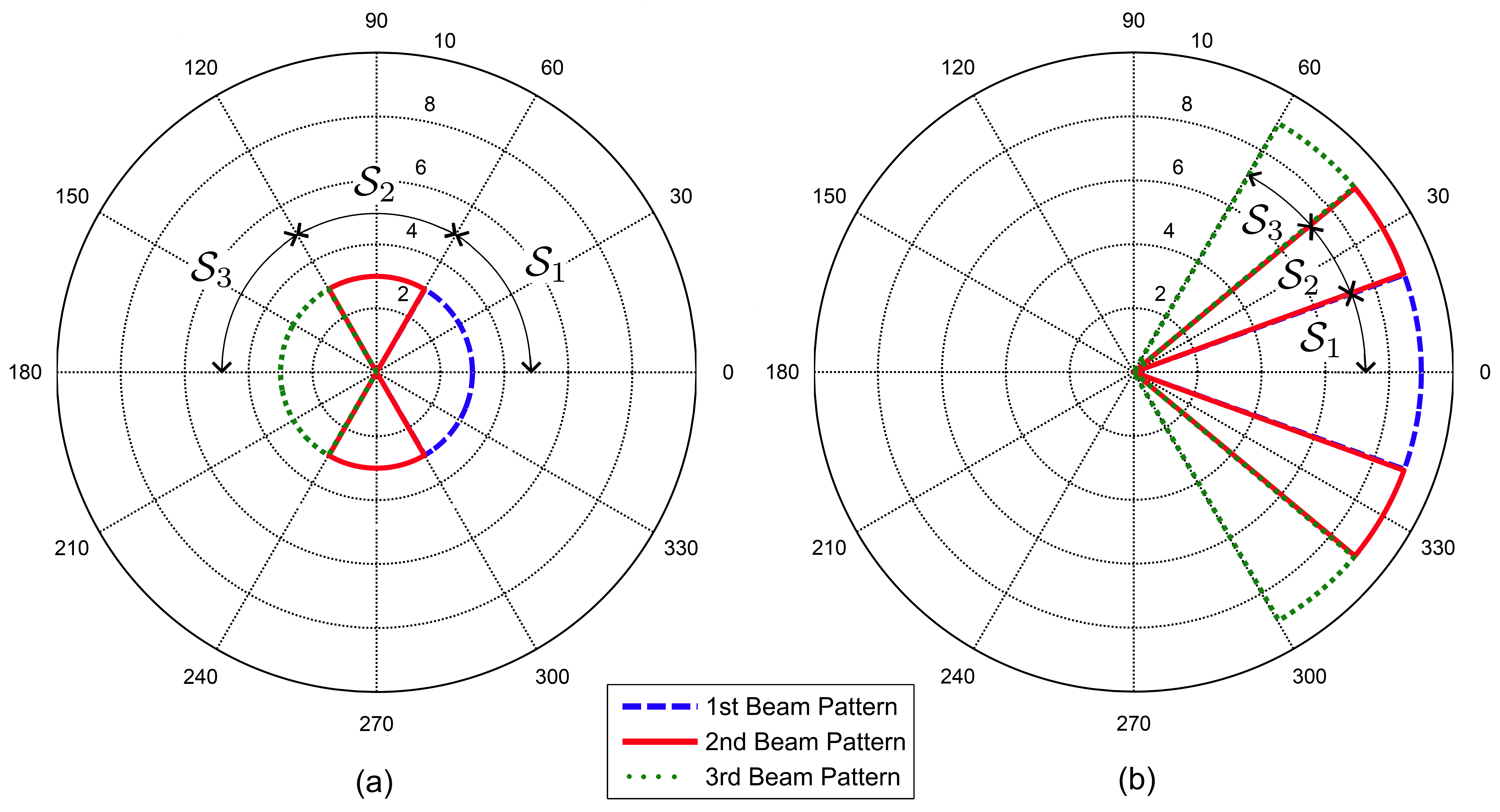
As one of the seminal works on multi-stage codebook approaches, [5] developed a “divide and conquer” search type algorithm to estimate sparse mmWave channels. As shown in Fig. 1, in each stage of this algorithm, the possible ranges of angles of departure (AODs) and angles of arrival (AOAs) are both divided into K<<Nmuch-less-than𝐾𝑁K<<N non-overlapped angular sub-ranges. Correspondingly, K𝐾K non-overlapped beam patterns are designed at both the transmitter and receiver such that each transmit (receive) beam pattern exactly covers one AOD (AOA) sub-range. The channel estimation carried out in each stage consists of K2superscript𝐾2K^{2} time slots. In each time slot, the pilot signal is transmitted using one of the K𝐾K beam patterns at the transmitter, and then collected by one of the K𝐾K beam patterns at the receiver. The corresponding channel output for each pair of transmit-receive beam patterns can then be obtained. These K2superscript𝐾2K^{2} time slots span all the combinations of transmit-receive beam patterns. By comparing the magnitudes of the corresponding K2superscript𝐾2K^{2} channel outputs, the transmit/receive sub-ranges that the AOD/AOA most likely belong to are determined. The receiver can then feed back the AOD information for use at the transmitter. Afterwards, the algorithm will limit the estimation to the angular sub-range identified at each link end in the previous stage and further divide it into K𝐾K sub-ranges for the channel estimation in the next stage. An example of multi-stage angular refinement, using our proposed approach, can be seen in Fig. 3. This process continues until the smallest beam width resolution is reached. It is shown in [5] that the algorithm requires estimation time proportional to K2logK(N)superscript𝐾2subscriptlog𝐾𝑁K^{2}\lceil\text{log}_{K}(N)\rceil per path. Despite the significant improvement when compared to the exhaustive search approach, such a channel estimation algorithm still might not be quick enough to track the fast channel variations, especially for mmWave mobile channels with rapidly changing parameters. Furthermore, at high SNR it may not be necessary to perform so many measurements, which would result in an unnecessary time delay. Adaptive training approaches are also investigated in [27, 28, 29, 30]. While these approaches are shown to significantly improve system performance as the number of measurement iterations is increased, there is generally no adaptation of the number of measurements with respect to the associated probability of success or channel conditions.
Refer to caption
Figure 1: Illustration of the beam patterns adopted in the first (a) and second (b) stages of the channel estimation algorithm of [5] when K=3𝐾3K=3. The three sub-ranges in the first stage are, [0,π/3)0𝜋3[0,\pi/3), [π/3,2π/3)𝜋32𝜋3[\pi/3,2\pi/3) and [2π/3,π)2𝜋3𝜋[2\pi/3,\pi), respectively. By assuming that the possible AOAs/AODs are reduced to the sub-range [0,π/3)0𝜋3[0,\pi/3) in the first stage, this sub-range is further divided into [0,π/9)0𝜋9[0,\pi/9), [π/9,2π/9)𝜋92𝜋9[\pi/9,2\pi/9) and [2π/9,π/3)2𝜋9𝜋3[2\pi/9,\pi/3), respectively, in the second stage.

Motivated by this, in this paper we develop a fast mmWave MIMO channel estimation framework by designing a set of novel overlapped beam patterns that can significantly reduce the number of channel estimation measurements. In order to improve estimation accuracy, we then introduce a novel rate-adaptive channel estimation approach, where the average number of channel measurements is adapted to channel conditions. The main contributions of this paper are summarized as follows:

  • Relying on novel overlapped beam pattern design, we first present a fast channel estimation (FCE) algorithm for mmWave systems. In this algorithm, we develop a maximum likelihood (ML) detector to optimally extract the channel AOD/AOA information from the measurements. We also design a linear minimum mean squared error (LMMSE) channel estimator to estimate the channel coefficients by optimally combining the selected measurements in all stages.

  • We then develop a rate-adaptive channel estimation (RACE) algorithm, in which additional measurements are permitted when the current measurements are found to have an inadequate probability of success. In this way, the number of measurements can adapt to the channel conditions and the channel estimation accuracy can be significantly improved with minimal measurements.

  • We analyze the probability of channel estimation error for the FCE algorithm. In particular, we derive a closed-form approximation, lower bound and upper bound for the PEE. Based on the Shannon-Hartley theorem, we also provide some theoretical analysis for the minimum energy required to estimate the channel using the RACE algorithm.

  • Finally, we compare the performance of the proposed algorithms to that of the algorithm in [5] with non-overlapped beam patterns. Simulation results show that both of the proposed algorithms can significantly reduce the number of channel measurements compared to [5]. We show that the FCE algorithm achieves a guaranteed reduction of channel measurements, at the expense of estimation accuracy. On the other hand, the RACE algorithm can achieve the same average reduction of channel measurements as the FCE algorithm, but using up to 6dB less signal energy compared to the algorithm in [5].

Notation : 𝑨𝑨\boldsymbol{A} is a matrix, 𝒂𝒂\boldsymbol{a} is a vector, a𝑎{a} is a scalar, and 𝒜𝒜\mathcal{A} is a set. 𝑨2subscriptnorm𝑨2||\boldsymbol{A}||_{2} is the 2-norm of 𝑨𝑨\boldsymbol{A}, det(𝑨)det𝑨\text{det}(\boldsymbol{A}) is the determinant of 𝑨𝑨\boldsymbol{A} and |𝒜|𝒜|\mathcal{A}| represents the cardinality of 𝒜𝒜\mathcal{A}. 𝑨Tsuperscript𝑨𝑇\boldsymbol{A}^{T}, 𝑨Hsuperscript𝑨𝐻\boldsymbol{A}^{H} and 𝑨superscript𝑨\boldsymbol{A}^{*} are the transpose, conjugate transpose and conjugate of 𝑨𝑨\boldsymbol{A}, respectively. For a square matrix 𝑨𝑨\boldsymbol{A}, 𝑨1superscript𝑨1\boldsymbol{A}^{-1} represents its inverse. We use diag(𝒂)diag𝒂\text{diag}({\boldsymbol{a}}) to denote a diagonal matrix with entries of 𝒂𝒂\boldsymbol{a} on its diagonal. 𝑰Nsubscript𝑰𝑁\boldsymbol{I}_{N} is the N×N𝑁𝑁N\times N identity matrix, 𝟏Nsubscript1𝑁\boldsymbol{1}_{N} is an N×1𝑁1N\times 1 all 111 column vector and \lceil\cdot\rceil denotes the ceiling function. 𝒞𝒩(𝒎,𝑹)𝒞𝒩𝒎𝑹\mathcal{C}\mathcal{N}(\boldsymbol{m},\boldsymbol{R}) is a complex Gaussian random vector with mean 𝒎𝒎\boldsymbol{m} and covariance matrix 𝑹𝑹\boldsymbol{R}. E[𝒂]Edelimited-[]𝒂\text{E}[\boldsymbol{a}] and Cov[𝒂]Covdelimited-[]𝒂\text{Cov}[\boldsymbol{a}] denote the expected value and covariance of 𝒂𝒂{\boldsymbol{a}}, respectively. 𝑨𝑩tensor-product𝑨𝑩\boldsymbol{A}\otimes\boldsymbol{B} denotes the Kronecker product of 𝑨𝑨\boldsymbol{A} and 𝑩𝑩\boldsymbol{B} whereas 𝑨𝑩direct-product𝑨𝑩\boldsymbol{A}\odot\boldsymbol{B} denotes the row-wise Kronecker product of 𝑨𝑨\boldsymbol{A} and 𝑩𝑩\boldsymbol{B}.

II System Model

Consider a mmWave MIMO system composed of Ntsubscript𝑁𝑡N_{t} transmit antennas and Nrsubscript𝑁𝑟N_{r} receive antennas. We consider that both the transmitter and receiver are equipped with a limited number of radio frequency (RF) chains. Following [5], we further assume that these RF chains, at one end, can only be combined to form a single beam pattern, indicating that only one pilot signal can be transmitted and received at one time. In this paper, for simplicity, we consider the unconstrained beamforming vectors by ignoring some practical constraints imposed by hardware such as constant amplitude and quantized phase shifters. However, in practice, our unconstrained beamforming vectors could be realized by using a network of constrained beamformers with quantized phase shifters and constant amplitude as the hybrid-beamforming approach adopted in [5] and depicted by Figure 2 therein. To estimate the channel matrix, the transmitter sends a pilot signal x𝑥x, with unit energy (x2=1subscriptnorm𝑥21||x||_{2}=1), to the receiver. Denote by 𝒇𝒇\boldsymbol{f} and 𝒘𝒘\boldsymbol{w} (𝒇2=𝒘2=1)subscriptnorm𝒇2subscriptnorm𝒘21(||\boldsymbol{f}||_{2}=||\boldsymbol{w}||_{2}=1), respectively, the Nt×1subscript𝑁𝑡1N_{t}\times 1 beamforming vector at the transmitter and Nr×1subscript𝑁𝑟1N_{r}\times 1 beamforming vector at the receiver. The corresponding channel output can be represented as

y=P𝒘H𝑯𝒇x+𝒘H𝒒,𝑦𝑃superscript𝒘𝐻𝑯𝒇𝑥superscript𝒘𝐻𝒒y=\sqrt{P}\boldsymbol{w}^{H}\boldsymbol{H}\boldsymbol{f}x+\boldsymbol{w}^{H}\boldsymbol{q}, (1)

where 𝑯𝑯\boldsymbol{H} denotes the Nr×Ntsubscript𝑁𝑟subscript𝑁𝑡N_{r}\times N_{t} MIMO channel matrix, P𝑃P is the transmit power and 𝒒𝒒\boldsymbol{q} is an Nr×1subscript𝑁𝑟1N_{r}\times 1 complex additive white Gaussian noise (AWGN) vector following distribution 𝒞𝒩(0,N0𝑰Nr)𝒞𝒩0subscript𝑁0subscript𝑰subscript𝑁𝑟\mathcal{C}\mathcal{N}(0,N_{0}\boldsymbol{I}_{N_{r}}).

In this paper we follow [31] and adopt a two-dimensional (2D) sparse geometric-based channel model. Specifically, we consider an L𝐿L-path channel between the transceiver, with the l𝑙lth path having steering AOD, ϕltsubscriptsuperscriptitalic-ϕ𝑡𝑙\phi^{t}_{l}, and AOA, ϕlrsubscriptsuperscriptitalic-ϕ𝑟𝑙\phi^{r}_{l} where l=1,,L𝑙1𝐿l=1,...,L. Then the corresponding channel matrix can be expressed in terms of the physical propagation path parameters as

𝑯=NtNrl=1Lαl𝒂r(ϕlr)𝒂tH(ϕlt)𝑯subscript𝑁𝑡subscript𝑁𝑟superscriptsubscript𝑙1𝐿subscript𝛼𝑙subscript𝒂𝑟superscriptsubscriptitalic-ϕ𝑙𝑟superscriptsubscript𝒂𝑡𝐻superscriptsubscriptitalic-ϕ𝑙𝑡\boldsymbol{H}=\sqrt{N_{t}N_{r}}\sum\limits_{l=1}^{L}\alpha_{l}\boldsymbol{a}_{r}(\phi_{l}^{r})\boldsymbol{a}_{t}^{H}(\phi_{l}^{t}) (2)

where αlsubscript𝛼𝑙\alpha_{l} is the fading coefficient of the l𝑙lth propagation path, and 𝒂t(ϕlt)subscript𝒂𝑡superscriptsubscriptitalic-ϕ𝑙𝑡\boldsymbol{a}_{t}(\phi_{l}^{t}) and 𝒂r(ϕlr)subscript𝒂𝑟superscriptsubscriptitalic-ϕ𝑙𝑟\boldsymbol{a}_{r}(\phi_{l}^{r}) respectively denote the transmit and receive spatial signatures of the l𝑙lth path. To simplify the analysis, we assume that the transmitter and receiver have the same number of antennas (i.e., Nt=Nr=Nsubscript𝑁𝑡subscript𝑁𝑟𝑁N_{t}=N_{r}=N). However, it is worth pointing out that the developed schemes can be easily extended to a general asymmetric system. If uniform linear antenna arrays (ULA) are employed at both the transmitter and receiver, we can define 𝒂t(ϕlt)=𝒖(ϕlt)subscript𝒂𝑡superscriptsubscriptitalic-ϕ𝑙𝑡𝒖superscriptsubscriptitalic-ϕ𝑙𝑡\boldsymbol{a}_{t}(\phi_{l}^{t})=\boldsymbol{u}(\phi_{l}^{t}) and 𝒂r(ϕlr)=𝒖(ϕlr)subscript𝒂𝑟superscriptsubscriptitalic-ϕ𝑙𝑟𝒖superscriptsubscriptitalic-ϕ𝑙𝑟\boldsymbol{a}_{r}(\phi_{l}^{r})=\boldsymbol{u}(\phi_{l}^{r}), respectively, where

𝒖(ϵ)1N[1,ej2πϵ,,ej2π(N1)ϵ]T.𝒖italic-ϵ1𝑁superscript1superscript𝑒𝑗2𝜋italic-ϵsuperscript𝑒𝑗2𝜋𝑁1italic-ϵ𝑇\boldsymbol{u}(\epsilon)\triangleq\frac{1}{\sqrt{N}}[1,e^{j2\pi\epsilon},\cdots,e^{j2\pi(N-1)\epsilon}]^{T}. (3)

Here, the steering angle, ϕltsuperscriptsubscriptitalic-ϕ𝑙𝑡\phi_{l}^{t}, is related to the physical angle θlt[0,π)superscriptsubscript𝜃𝑙𝑡0𝜋\theta_{l}^{t}\in[0,\pi) by ϕlt=d sin(θlt)λsuperscriptsubscriptitalic-ϕ𝑙𝑡𝑑 sinsuperscriptsubscript𝜃𝑙𝑡𝜆\phi_{l}^{t}=\frac{d\text{ sin}(\theta_{l}^{t})}{\lambda} with λ𝜆\lambda denoting the signal wavelength111Note that the use of ULA results in no distinguishable difference between AODs θltsuperscriptsubscript𝜃𝑙𝑡\theta_{l}^{t} and θltsuperscriptsubscript𝜃𝑙𝑡-\theta_{l}^{t} or between AOAs θlrsuperscriptsubscript𝜃𝑙𝑟\theta_{l}^{r} and θlrsuperscriptsubscript𝜃𝑙𝑟-\theta_{l}^{r}. Hence, only AODs and AOAs in the range [0,π)0𝜋[0,\pi) need to be considered.. A similar expression can be written for ϕlrsuperscriptsubscriptitalic-ϕ𝑙𝑟\phi_{l}^{r} at the receiver. With half-wavelength spacing, the distance between antenna elements becomes d=λ/2𝑑𝜆2d=\lambda/2.

From (2), we can see that the overall channel state information of each path includes only three parameters, i.e., the AOD ϕlrsuperscriptsubscriptitalic-ϕ𝑙𝑟\phi_{l}^{r}, the AOA ϕlrsuperscriptsubscriptitalic-ϕ𝑙𝑟\phi_{l}^{r}, and the fading coefficient αlsubscript𝛼𝑙\alpha_{l}. We assume that the fading coefficient of each path follows a complex Gaussian distribution with zero mean and variance PRsubscript𝑃𝑅P_{R} and that both ϕltsuperscriptsubscriptitalic-ϕ𝑙𝑡\phi_{l}^{t} and ϕlrsuperscriptsubscriptitalic-ϕ𝑙𝑟\phi_{l}^{r} can only take some discrete values from the set 𝒰N={0,πN,,π(N1)N}subscript𝒰𝑁0𝜋𝑁𝜋𝑁1𝑁\mathcal{U}_{N}=\{0,\frac{\pi}{N},\cdots,\frac{\pi(N-1)}{N}\}. Here, for the sake of ensuing mathematical problem formulation, we only consider the discrete AOA and AOD. It is noteworthy that they can be continuous in practice. However, the extension to the case with continuous AOD/AOA may require the consideration of other more practical issues such as the number of RF chains to realize the beam patterns and the hardware constraints (e.g., quantized phase shifters) imposed on the RF beamforming vectors, which may constitute a new paper. We thus have left this extension as our future work.

We aim to find an efficient way to estimate the three parameters for each path. The key challenge here is how to design a sequence of 𝒇ssuperscript𝒇𝑠\boldsymbol{f}^{\prime}s and 𝒘ssuperscript𝒘𝑠\boldsymbol{w}^{\prime}s in such a way that the channel parameters can be quickly and accurately estimated. We consider M𝑀M pairs of beam patterns that are designed to span all possible transmit-receive combinations. Denote by 𝒇msubscript𝒇𝑚\boldsymbol{f}_{m} and 𝒘msubscript𝒘𝑚\boldsymbol{w}_{m}, respectively, the transmit and receive beamforming vectors adopted in the m𝑚mth channel measurement time slot such that 𝒇m2=𝒘m2=1,m=1,,Mformulae-sequencesubscriptnormsubscript𝒇𝑚2subscriptnormsubscript𝒘𝑚21for-all𝑚1𝑀||\boldsymbol{f}_{m}||_{2}=||\boldsymbol{w}_{m}||_{2}=1,\;\forall\;m=1,\cdots,M. Similarly to [5], we assume the same pilot symbol x𝑥x is transmitted during the M𝑀M time slots. Then, after M𝑀M time slots, we can obtain a sequence of M𝑀M measurements represented as

𝒚=𝒚absent\displaystyle\boldsymbol{y}= Px𝒉v+𝒏,𝑃𝑥subscript𝒉𝑣𝒏\displaystyle\sqrt{P}x\boldsymbol{h}_{v}+\boldsymbol{n}, (4)

where 𝒉vsubscript𝒉𝑣\boldsymbol{h}_{v} describes the channel input-output relationship for a given set of transmit and receive beamforming vectors defined by

𝒉v=[𝒘1H𝑯𝒇1𝒘2H𝑯𝒇2𝒘MH𝑯𝒇M]subscript𝒉𝑣delimited-[]superscriptsubscript𝒘1𝐻𝑯subscript𝒇1missing-subexpressionmissing-subexpressionsuperscriptsubscript𝒘2𝐻𝑯subscript𝒇2missing-subexpressionmissing-subexpressionmissing-subexpressionmissing-subexpressionsuperscriptsubscript𝒘𝑀𝐻𝑯subscript𝒇𝑀missing-subexpressionmissing-subexpression\displaystyle\boldsymbol{h}_{v}=\left[\begin{array}[]{ccc}\boldsymbol{w}_{1}^{H}\boldsymbol{H}\boldsymbol{f}_{1}\\ \boldsymbol{w}_{2}^{H}\boldsymbol{H}\boldsymbol{f}_{2}\\ \vdots\\ \boldsymbol{w}_{M}^{H}\boldsymbol{H}\boldsymbol{f}_{M}\end{array}\right] (9)

and

𝒏=[𝒘1H𝒒1𝒘2H𝒒2𝒘MH𝒒M]𝒏delimited-[]subscriptsuperscript𝒘𝐻1subscript𝒒1missing-subexpressionmissing-subexpressionsubscriptsuperscript𝒘𝐻2subscript𝒒2missing-subexpressionmissing-subexpressionmissing-subexpressionmissing-subexpressionsubscriptsuperscript𝒘𝐻𝑀subscript𝒒𝑀missing-subexpressionmissing-subexpression\displaystyle\boldsymbol{n}=\left[\begin{array}[]{ccc}\boldsymbol{w}^{H}_{1}\boldsymbol{q}_{1}\\ \boldsymbol{w}^{H}_{2}\boldsymbol{q}_{2}\\ \vdots\\ \boldsymbol{w}^{H}_{M}\boldsymbol{q}_{M}\end{array}\right] (14)

is an M×1𝑀1M\times 1 vector of the corresponding noise terms. Note that since 𝒘m2=1subscriptnormsubscript𝒘𝑚21||\boldsymbol{w}_{m}||_{2}=1, for-all\forall m𝑚m, the vector 𝒏𝒏\boldsymbol{n} follows the same distribution as that of 𝒒msubscript𝒒𝑚{\boldsymbol{q}_{m}}, i.e., 𝒏𝒞𝒩(0,N0IM)similar-to𝒏𝒞𝒩0subscript𝑁0subscript𝐼𝑀\boldsymbol{n}\sim\mathcal{C}\mathcal{N}(0,N_{0}I_{M}).

Motivated by the geometric sparsity of the mmWave channel, in the following two sections, we propose to use a set of overlapped beam patterns that are able to estimate the AOD/AOA information very quickly. We then extend the algorithm to use a rate-adaptive estimation approach. The adaptive nature of the algorithm permits additional measurements to be performed under poor channel conditions. This allows the fast channel estimation to be carried out with significant accuracy and energy efficiency.

III Fast Channel Estimation with Overlapped Beam Patterns

In this section, we develop a fast channel estimation framework for mmWave systems using overlapped beam patterns, as illustrated in Fig. 3. Specifically, we design a set of beam patterns that are adopted in different measurement time intervals and are overlapped with one another in the angular domain. A maximum likelihood based estimation algorithm is then proposed to accurately retrieve the channel state information from the set of measurements. The proposed channel estimation algorithm also works in a similar multi-stage manner as that in [5] where each stage reduces the possible sub-ranges in which the AOD/AOA are expected to be found.

III-A An Example of Overlapped Beam Pattern Design

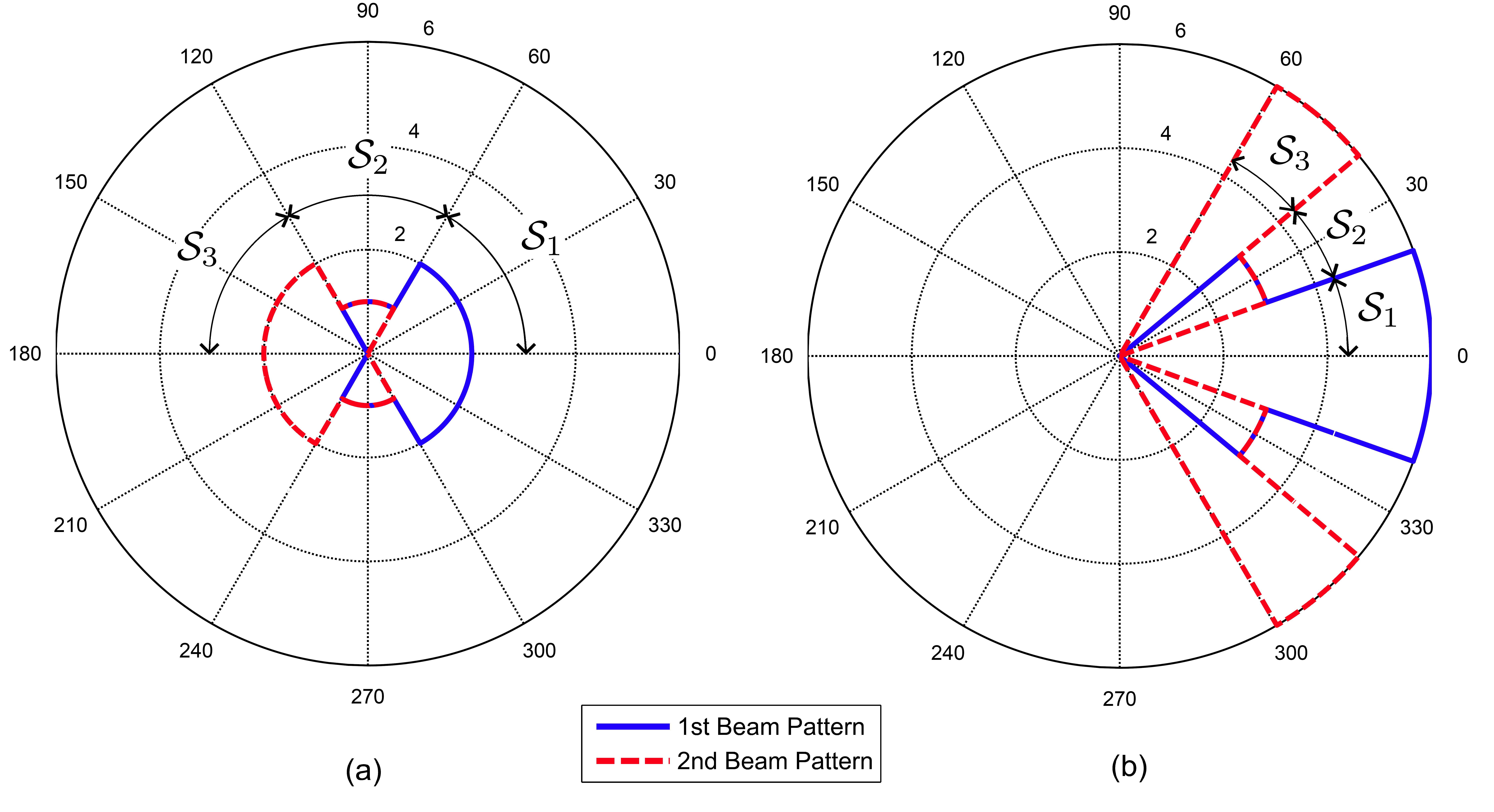
We will first explain the design principle of overlapped beam patterns using a simple example. Following Fig. 1, we divide the AOD/AOA angular spaces into K=3𝐾3K=3 sub-ranges in the first stage, denoted by 𝒮1={ϵ𝒰N|0ϵ<π/3}subscript𝒮1conditional-setitalic-ϵsubscript𝒰𝑁0italic-ϵ𝜋3\mathcal{S}_{1}=\{\epsilon\in\mathcal{U}_{N}|0\leq\epsilon<\pi/3\}, 𝒮2={ϵ𝒰N|π/3ϵ<2π/3}subscript𝒮2conditional-setitalic-ϵsubscript𝒰𝑁𝜋3italic-ϵ2𝜋3\mathcal{S}_{2}=\{\epsilon\in\mathcal{U}_{N}|\pi/3\leq\epsilon<2\pi/3\} and 𝒮3={ϵ𝒰N|2π/3ϵ<π}subscript𝒮3conditional-setitalic-ϵsubscript𝒰𝑁2𝜋3italic-ϵ𝜋\mathcal{S}_{3}=\{\epsilon\in\mathcal{U}_{N}|2\pi/3\leq\epsilon<\pi\}, respectively. However, instead of using 3 beam patterns to cover them at each transceiver end as in Fig. 1(a), we propose to use only 2 overlapped beam patterns to achieve this. Fig. 2(a) illustrates our designed beam patterns in the first stage. We can see that the first and second beam patterns cover 𝒮1subscript𝒮1\mathcal{S}_{1}, 𝒮2subscript𝒮2\mathcal{S}_{2} and 𝒮2subscript𝒮2\mathcal{S}_{2}, 𝒮3subscript𝒮3\mathcal{S}_{3}, respectively, and are overlapped in the whole range of 𝒮2subscript𝒮2\mathcal{S}_{2}. Intuitively, if a path is observed in two measurements using adjacent beam patterns, the AOD or AOA must belong to the overlapped sub-range of these two beam patterns. It is also seen that each beam pattern can have different amplitudes in different sub-ranges. We represent the amplitudes of each beam pattern in different sub-ranges by a vector. For beam pattern 1 and 2 in Fig. 2(a), these vectors are respectively defined as

𝒃1=[b1,1,b1,2,b1,3],𝒃2=[b2,1,b2,2,b2,3]formulae-sequencesubscript𝒃1delimited-[]subscript𝑏11subscript𝑏12subscript𝑏13subscript𝒃2delimited-[]subscript𝑏21subscript𝑏22subscript𝑏23\boldsymbol{b}_{1}=\left[\begin{array}[]{ccc}b_{1,1},&b_{1,2},&b_{1,3}\\ \end{array}\right],\;\\ \boldsymbol{b}_{2}=\left[\begin{array}[]{ccc}b_{2,1},&b_{2,2},&b_{2,3}\end{array}\right] (15)

where 𝒃isubscript𝒃𝑖\boldsymbol{b}_{i} corresponds to the i𝑖ith beam pattern with bi,ksubscript𝑏𝑖𝑘b_{i,k} denoting the amplitude of the i𝑖ith beam pattern in sub-range Sk,k=1,,Kformulae-sequencesubscript𝑆𝑘for-all𝑘1𝐾S_{k},\;\forall\;k=1,...,K. By using M=4𝑀4M=4 measurement time slots, we can then span all beam pattern combinations between the transceiver. We denote the sequential set of beam patterns respectively adopted at the transmitter and receiver by
Refer to caption
Figure 2: Illustration of the overlapped beam patterns adopted in the first (a) and second (b) stages of the proposed algorithm when K=3𝐾3K=3. By assuming that the possible AOAs/AODs are reduced to the sub-range [0,π/3)0𝜋3[0,\pi/3) in the first stage, this sub-range is further divided into [0,π/9)0𝜋9[0,\pi/9), [π/9,2π/9)𝜋92𝜋9[\pi/9,2\pi/9) and [2π/9,π/3)2𝜋9𝜋3[2\pi/9,\pi/3), respectively, in the second stage.
𝑩T(M)=[𝒃1𝒃1𝒃2𝒃2]=[b1,1,b1,2,b1,3b1,1,b1,2,b1,3b2,1,b2,2,b2,3b2,1,b2,2,b2,3],superscriptsubscript𝑩𝑇𝑀delimited-[]subscript𝒃1missing-subexpressionmissing-subexpressionsubscript𝒃1missing-subexpressionmissing-subexpressionsubscript𝒃2missing-subexpressionmissing-subexpressionsubscript𝒃2missing-subexpressionmissing-subexpressiondelimited-[]subscript𝑏11subscript𝑏12subscript𝑏13subscript𝑏11subscript𝑏12subscript𝑏13subscript𝑏21subscript𝑏22subscript𝑏23subscript𝑏21subscript𝑏22subscript𝑏23\displaystyle\boldsymbol{B}_{T}^{(M)}=\left[\begin{array}[]{ccc}\boldsymbol{b}_{1}\\ \boldsymbol{b}_{1}\\ \boldsymbol{b}_{2}\\ \boldsymbol{b}_{2}\end{array}\right]=\left[\begin{array}[]{ccc}b_{1,1},&b_{1,2},&b_{1,3}\\ b_{1,1},&b_{1,2},&b_{1,3}\\ b_{2,1},&b_{2,2},&b_{2,3}\\ b_{2,1},&b_{2,2},&b_{2,3}\end{array}\right], (24)
𝑩R(M)=[𝒃1𝒃2𝒃1𝒃2]=[b1,1,b1,2,b1,3b2,1,b2,2,b2,3b1,1,b1,2,b1,3b2,1,b2,2,b2,3].superscriptsubscript𝑩𝑅𝑀delimited-[]subscript𝒃1missing-subexpressionmissing-subexpressionsubscript𝒃2missing-subexpressionmissing-subexpressionsubscript𝒃1missing-subexpressionmissing-subexpressionsubscript𝒃2missing-subexpressionmissing-subexpressiondelimited-[]subscript𝑏11subscript𝑏12subscript𝑏13subscript𝑏21subscript𝑏22subscript𝑏23subscript𝑏11subscript𝑏12subscript𝑏13subscript𝑏21subscript𝑏22subscript𝑏23\displaystyle\boldsymbol{B}_{R}^{(M)}=\left[\begin{array}[]{ccc}\boldsymbol{b}_{1}\\ \boldsymbol{b}_{2}\\ \boldsymbol{b}_{1}\\ \boldsymbol{b}_{2}\\ \end{array}\right]=\left[\begin{array}[]{ccc}b_{1,1},&b_{1,2},&b_{1,3}\\ b_{2,1},&b_{2,2},&b_{2,3}\\ b_{1,1},&b_{1,2},&b_{1,3}\\ b_{2,1},&b_{2,2},&b_{2,3}\end{array}\right]. (33)

We refer to these as the beam pattern design matrices, with their m𝑚mth row denoting the beam pattern adopted in the m𝑚mth measurement time slot, where m=1,,M𝑚1𝑀m=1,...,M. The efficient design of these beam patterns can lead to many solutions. However, one desirable property is that the same quantity of signal energy is transmitted/received via each sub-range over all measurements, i.e., the energy of each column of (24)-(33) should have the same Euclidean norm. This provides the same accuracy for each possible sub-range combination. Another desirable property is that the transmit/receive beamforming gains of all measurement patterns are equal, i.e., the energy of each rows of (24)-(33) should be the same.

One possible way to make the beam pattern sub-range amplitudes in (15) follow the aforementioned properties, is to normalize 𝑩T(M)subscriptsuperscript𝑩𝑀𝑇\boldsymbol{B}^{(M)}_{T} and 𝑩R(M)subscriptsuperscript𝑩𝑀𝑅\boldsymbol{B}^{(M)}_{R} to have unit energy in each row and have equal energy in each column. For the beam patterns in Fig. 2, we have b1,3=b2,1=0subscript𝑏13subscript𝑏210b_{1,3}=b_{2,1}=0, as beam patterns 111 and 222 do not cover, respectively, the third and first sub-ranges. Due to the symmetry between the two beam patterns, we further have b1,1=b2,3=β1subscript𝑏11subscript𝑏23subscript𝛽1b_{1,1}=b_{2,3}=\beta_{1} and b1,2=b2,2=β2subscript𝑏12subscript𝑏22subscript𝛽2b_{1,2}=b_{2,2}=\beta_{2}. This leads to β1=13subscript𝛽113\beta_{1}=\frac{{1}}{\sqrt{3}} and β2=23subscript𝛽223\beta_{2}=\frac{\sqrt{2}}{\sqrt{3}}, and the matrices in (24)-(33) become

𝑩T(M)=[23130231300132301323],𝑩R(M)=[23130013232313001323].formulae-sequencesuperscriptsubscript𝑩𝑇𝑀delimited-[]23130231300132301323superscriptsubscript𝑩𝑅𝑀delimited-[]23130013232313001323\displaystyle\boldsymbol{B}_{T}^{(M)}=\left[\begin{array}[]{ccc}\frac{\sqrt{2}}{\sqrt{3}}&\frac{{1}}{\sqrt{3}}&0\\ \frac{\sqrt{2}}{\sqrt{3}}&\frac{{1}}{\sqrt{3}}&0\\ 0&\frac{{1}}{\sqrt{3}}&\frac{\sqrt{2}}{\sqrt{3}}\\ 0&\frac{{1}}{\sqrt{3}}&\frac{\sqrt{2}}{\sqrt{3}}\end{array}\right],\;\boldsymbol{B}_{R}^{(M)}=\left[\begin{array}[]{ccc}\frac{\sqrt{2}}{\sqrt{3}}&\frac{{1}}{\sqrt{3}}&0\\ 0&\frac{{1}}{\sqrt{3}}&\frac{\sqrt{2}}{\sqrt{3}}\\ \frac{\sqrt{2}}{\sqrt{3}}&\frac{{1}}{\sqrt{3}}&0\\ 0&\frac{{1}}{\sqrt{3}}&\frac{\sqrt{2}}{\sqrt{3}}\end{array}\right]. (42)

In order to observe the resultant amplitude gains (i.e., the transceiver gain) over each of the K2=9superscript𝐾29K^{2}=9 sub-range combinations, we introduce another matrix referred to as the generator matrix. We define this as the row-wise Kronecker product between the transmit beam pattern design matrix and the receive beam pattern design matrix such that
Refer to caption
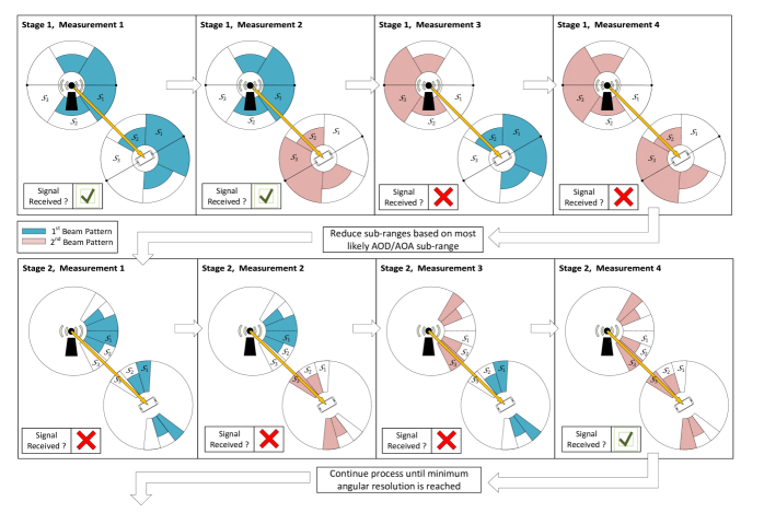
Figure 3: Illustration of multi-stage channel estimation using the example overlapped beam patterns. Here we use an arrow to represent the propagation path to be estimated. As can be seen, in the first stage, it is expected that a signal will only be received in the first and second measurements (due to the propagation path angle). As the transmit beam patterns used are predetermined and thus known to the receiver, it can be logically deduced that the AOD at the transmitter can only belong to the 1st sub-range and that the AOA at the receiver should belong to the 2nd sub-range. It is noteworthy that this series of measurements (i.e., [✓,✓,✗,✗]) corresponds to the 2nd column of the generator matrix in (53). The receiver then feeds back the AOD sub-range to the transmitter for the channel estimation in next stage. Both the transceiver and receiver then divide their estimated sub-range into narrower sub-ranges and carry out further overlapped sub-range measurements. As can be seen, in the second stage, it is expected that a signal will only be received in the final measurement. Logically, this means that the AOD at the transmitter is within the 3rd sub-range and the AOA at the receiver is on the 3rd sub-range. This series of measurements (i.e., [✗, ✗, ✗, ✓]) also corresponds to the 9th column of the generator matrix in (53).
𝑮(M)superscript𝑮𝑀\displaystyle\boldsymbol{G}^{(M)} =𝑩T(M)𝑩R(M)=[𝒃1𝒃1𝒃1𝒃2𝒃2𝒃1𝒃2𝒃2]absentdirect-productsuperscriptsubscript𝑩𝑇𝑀superscriptsubscript𝑩𝑅𝑀delimited-[]tensor-productsubscript𝒃1subscript𝒃1missing-subexpressionmissing-subexpressiontensor-productsubscript𝒃1subscript𝒃2missing-subexpressionmissing-subexpressiontensor-productsubscript𝒃2subscript𝒃1missing-subexpressionmissing-subexpressiontensor-productsubscript𝒃2subscript𝒃2missing-subexpressionmissing-subexpression\displaystyle=\boldsymbol{B}_{T}^{(M)}\odot\;\boldsymbol{B}_{R}^{(M)}=\left[\begin{array}[]{ccc}\boldsymbol{b}_{1}\otimes\boldsymbol{b}_{1}\\ \boldsymbol{b}_{1}\otimes\boldsymbol{b}_{2}\\ \boldsymbol{b}_{2}\otimes\boldsymbol{b}_{1}\\ \boldsymbol{b}_{2}\otimes\boldsymbol{b}_{2}\\ \end{array}\right] (48)
=13[220210000022012000000210220000012022],absent13delimited-[]220210000022012000000210220000012022\displaystyle=\frac{1}{3}\left[\begin{array}[]{ccccccccc}2&\sqrt{2}&0&\sqrt{2}&{1}&0&0&0&0\\ 0&\sqrt{2}&2&0&1&\sqrt{2}&0&0&0\\ 0&0&0&\sqrt{2}&1&0&2&\sqrt{2}&0\\ 0&0&0&0&1&\sqrt{2}&0&\sqrt{2}&2\end{array}\right], (53)

recalling that direct-product\odot and tensor-product\otimes represent the row-wise Kronecker and Kronecker product operations, respectively. By denoting bT(m,kt)subscriptsuperscript𝑏𝑚superscript𝑘𝑡𝑇{b}^{(m,k^{t})}_{T} and bR(m,kr)subscriptsuperscript𝑏𝑚superscript𝑘𝑟𝑅{b}^{(m,k^{r})}_{R} as the entry on the ktsuperscript𝑘𝑡k^{t}th and krsuperscript𝑘𝑟k^{r}th column on the m𝑚mth row in 𝑩T(M)superscriptsubscript𝑩𝑇𝑀\boldsymbol{B}_{T}^{(M)} and 𝑩R(M)superscriptsubscript𝑩𝑅𝑀\boldsymbol{B}_{R}^{(M)}, respectively, we can express the d𝑑dth column of 𝑮(M)superscript𝑮𝑀\boldsymbol{G}^{(M)} as

𝑮d(M)=[bT(1,kt)bR(1,kr)bT(M,kt)bR(M,kr)]subscriptsuperscript𝑮𝑀𝑑delimited-[]subscriptsuperscript𝑏1superscript𝑘𝑡𝑇subscriptsuperscript𝑏1superscript𝑘𝑟𝑅missing-subexpressionmissing-subexpressionmissing-subexpressionmissing-subexpressionsubscriptsuperscript𝑏𝑀superscript𝑘𝑡𝑇subscriptsuperscript𝑏𝑀superscript𝑘𝑟𝑅missing-subexpressionmissing-subexpression\displaystyle\boldsymbol{G}^{(M)}_{d}=\left[\begin{array}[]{ccc}{b}^{(1,k^{t})}_{T}{b}^{(1,k^{r})}_{R}\\ \vdots\\ {b}^{(M,k^{t})}_{T}{b}^{(M,k^{r})}_{R}\\ \end{array}\right] (58)

where the relationship d=K(kt1)+kr𝑑𝐾superscript𝑘𝑡1superscript𝑘𝑟d=K(k^{t}-1)+k^{r} is a result of the Kronecker product operation.

The columns of generator matrix describe the M=4𝑀4M=4 received measurement gains over each of the K2=9superscript𝐾29K^{2}=9 sub-range combinations. For example, if a path were present between the transmit sub-range kt=3superscript𝑘𝑡3k^{t}=3 and the receive sub-range kr=1superscript𝑘𝑟1k^{r}=1, the measurement vector 𝒚𝒚\boldsymbol{y} would be expected to be a scalar multiple of column d=7𝑑7d=7 of 𝑮(M)superscript𝑮𝑀\boldsymbol{G}^{(M)}, expressed as 𝑮7(M)subscriptsuperscript𝑮𝑀7\boldsymbol{G}^{(M)}_{7}. It is important to note that the sets of beam patterns used in this paper are not unique. We later show that their performance, in terms of PEE, depends only on the Euclidean distance between each column of 𝑮(M)superscript𝑮𝑀\boldsymbol{G}^{(M)}, which directly determines the probability that one column corresponding to a certain sub-range is to be mistaken for another. In the example set shown in (53), each column has the same equal minimum Euclidean distance when compared with all other columns, although some have more spatial neighbours at this minimum distance than others.

III-B Beamforming Vector Design

To generate the beam patterns illustrated in Fig. 2(a) and described in (42), the transmit and receive beamforming vectors should be designed as follows. Denote by 𝒇msubscript𝒇𝑚\boldsymbol{f}_{m} and 𝒘msubscript𝒘𝑚\boldsymbol{w}_{m}, respectively, the transmit beamforming vector and receive beamforming vector corresponding to the m𝑚mth pair of beam patterns in 𝑩T(M)subscriptsuperscript𝑩𝑀𝑇\boldsymbol{B}^{(M)}_{T} and 𝑩R(M)subscriptsuperscript𝑩𝑀𝑅\boldsymbol{B}^{(M)}_{R}. We then design the product of the transmit array response and transmit beamforming vector to have

𝒖H(ϵ)𝒇m=CbT(m,k), if k{1,2,,K},ϵ𝒮k,superscript𝒖𝐻italic-ϵsubscript𝒇𝑚𝐶subscriptsuperscript𝑏𝑚𝑘𝑇 if k{1,2,,K},ϵ𝒮k\boldsymbol{u}^{H}(\epsilon)\boldsymbol{f}_{m}=C{b}^{(m,k)}_{T},\text{ if $\exists\;k\in\{1,2,...,K\},\epsilon\in\mathcal{S}_{k}$}, (59)

and the product of the receiver array response and receive beamforming vector to have

𝒖H(ϵ)𝒘m=CbR(m,k), if k{1,2,,K},ϵ𝒮k,superscript𝒖𝐻italic-ϵsubscript𝒘𝑚𝐶subscriptsuperscript𝑏𝑚𝑘𝑅 if k{1,2,,K},ϵ𝒮k\boldsymbol{u}^{H}(\epsilon)\boldsymbol{w}_{m}=C{b}^{(m,k)}_{R},\text{ if $\exists\;k\in\{1,2,...,K\},\epsilon\in\mathcal{S}_{k}$}, (60)

where 𝒖(ϵ)𝒖italic-ϵ\boldsymbol{u}(\epsilon) has been defined in (3) and C𝐶C is a scalar constant that ensures 𝒇m2=𝒘m2=1subscriptnormsubscript𝒇𝑚2subscriptnormsubscript𝒘𝑚21||\boldsymbol{f}_{m}||_{2}=||\boldsymbol{w}_{m}||_{2}=1. Physically, C𝐶C corresponds to the average directivity gain of each beam pattern and is the same for all m=1,,M𝑚1𝑀m=1,\cdots,M due to the normalization of the rows in (42). Eqs. (59) and (60) can be expressed in a matrix form as

𝑼H𝒇m=[CbT(m,1)𝟏|S1|CbT(m,K)𝟏|SK|]𝒛T(m)superscript𝑼𝐻subscript𝒇𝑚delimited-[]𝐶subscriptsuperscript𝑏𝑚1𝑇subscript1subscript𝑆1missing-subexpressionmissing-subexpressionmissing-subexpressionmissing-subexpression𝐶subscriptsuperscript𝑏𝑚𝐾𝑇subscript1subscript𝑆𝐾missing-subexpressionmissing-subexpressionsuperscriptsubscript𝒛𝑇𝑚\boldsymbol{U}^{H}\boldsymbol{f}_{m}=\left[\begin{array}[]{ccc}C{b}^{(m,1)}_{T}\boldsymbol{1}_{|S_{1}|}\\ \vdots\\ C{b}^{(m,K)}_{T}\boldsymbol{1}_{|S_{K}|}\end{array}\right]\triangleq\boldsymbol{z}_{T}^{(m)} (61)

and

𝑼H𝒘m=[CbR(m,1)𝟏|S1|CbR(m,K)𝟏|SK|]𝒛R(m)superscript𝑼𝐻subscript𝒘𝑚delimited-[]𝐶subscriptsuperscript𝑏𝑚1𝑅subscript1subscript𝑆1missing-subexpressionmissing-subexpressionmissing-subexpressionmissing-subexpression𝐶subscriptsuperscript𝑏𝑚𝐾𝑅subscript1subscript𝑆𝐾missing-subexpressionmissing-subexpressionsuperscriptsubscript𝒛𝑅𝑚\boldsymbol{U}^{H}\boldsymbol{w}_{m}=\left[\begin{array}[]{ccc}C{b}^{(m,1)}_{R}\boldsymbol{1}_{|S_{1}|}\\ \vdots\\ C{b}^{(m,K)}_{R}\boldsymbol{1}_{|S_{K}|}\end{array}\right]\triangleq\boldsymbol{z}_{R}^{(m)} (62)

where |𝒮|𝒮\left|\mathcal{S}\right| denotes the cardinality of set 𝒮𝒮\mathcal{S} and 𝑼=[𝒖(0),𝒖(πN),,𝒖(π(N1)N)]𝑼𝒖0𝒖𝜋𝑁𝒖𝜋𝑁1𝑁\boldsymbol{U}=\big{[}\boldsymbol{u}(0),\boldsymbol{u}\Big{(}\frac{\pi}{N}\Big{)},\cdots,\boldsymbol{u}\Big{(}\frac{\pi(N-1)}{N}\Big{)}\big{]} is a matrix whose columns describe the antenna array response at each angle. Therefore 𝒇msubscript𝒇𝑚\boldsymbol{f}_{m} and 𝒘msubscript𝒘𝑚\boldsymbol{w}_{m} can be designed as

𝒇m=(𝑼𝑼H)1𝑼𝒛T(m)subscript𝒇𝑚superscript𝑼superscript𝑼𝐻1𝑼superscriptsubscript𝒛𝑇𝑚\displaystyle\boldsymbol{f}_{m}=(\boldsymbol{U}\boldsymbol{U}^{H})^{-1}\boldsymbol{U}\boldsymbol{z}_{T}^{(m)} (63)

and

𝒘m=(𝑼𝑼H)1𝑼𝒛R(m)subscript𝒘𝑚superscript𝑼superscript𝑼𝐻1𝑼superscriptsubscript𝒛𝑅𝑚\displaystyle\boldsymbol{w}_{m}=(\boldsymbol{U}\boldsymbol{U}^{H})^{-1}\boldsymbol{U}\boldsymbol{z}_{R}^{(m)} (64)

where (𝑼𝑼H)1𝑼superscript𝑼superscript𝑼𝐻1𝑼(\boldsymbol{U}\boldsymbol{U}^{H})^{-1}\boldsymbol{U} is the pseudo inverse of 𝑼𝑼\boldsymbol{U}.

III-C Channel Measurements

We now perform channel estimation in the first stage using the previously designed transmit and receive beamforming vectors {𝒇m}subscript𝒇𝑚\{\boldsymbol{f}_{m}\} and {𝒘m}subscript𝒘𝑚\{\boldsymbol{w}_{m}\}. In each time slot, the beamforming vectors 𝒇msubscript𝒇𝑚\boldsymbol{f}_{m} and 𝒘msubscript𝒘𝑚\boldsymbol{w}_{m} are adopted to transmit/receive the pilot signal x𝑥x. If we substitute the channel in (2) into (9), we get

𝒉v(M)=xNl=1Lαl[(𝒂rH(ϕlr)𝒘1)H𝒂tH(ϕlt)𝒇1(𝒂rH(ϕlr)𝒘M)H𝒂tH(ϕlt)𝒇M].superscriptsubscript𝒉𝑣𝑀𝑥𝑁superscriptsubscript𝑙1𝐿subscript𝛼𝑙delimited-[]superscriptsubscriptsuperscript𝒂𝐻𝑟superscriptsubscriptitalic-ϕ𝑙𝑟subscript𝒘1𝐻superscriptsubscript𝒂𝑡𝐻superscriptsubscriptitalic-ϕ𝑙𝑡subscript𝒇1missing-subexpressionmissing-subexpressionmissing-subexpressionmissing-subexpressionsuperscriptsubscriptsuperscript𝒂𝐻𝑟superscriptsubscriptitalic-ϕ𝑙𝑟subscript𝒘𝑀𝐻superscriptsubscript𝒂𝑡𝐻superscriptsubscriptitalic-ϕ𝑙𝑡subscript𝒇𝑀missing-subexpressionmissing-subexpression\displaystyle\boldsymbol{h}_{v}^{(M)}=xN\sum\limits_{l=1}^{L}\alpha_{l}\left[\begin{array}[]{ccc}(\boldsymbol{a}^{H}_{r}(\phi_{l}^{r})\boldsymbol{w}_{1})^{H}\boldsymbol{a}_{t}^{H}(\phi_{l}^{t})\boldsymbol{f}_{1}\\ \vdots\\ (\boldsymbol{a}^{H}_{r}(\phi_{l}^{r})\boldsymbol{w}_{M})^{H}\boldsymbol{a}_{t}^{H}(\phi_{l}^{t})\boldsymbol{f}_{M}\end{array}\right]. (68)

Without loss of generality, let us consider the case with AOD, ϕlt𝒮kltsuperscriptsubscriptitalic-ϕ𝑙𝑡subscript𝒮superscriptsubscript𝑘𝑙𝑡\phi_{l}^{t}\in\mathcal{S}_{k_{l}^{t}} and AOA, ϕlr𝒮klrsuperscriptsubscriptitalic-ϕ𝑙𝑟subscript𝒮superscriptsubscript𝑘𝑙𝑟\phi_{l}^{r}\in\mathcal{S}_{k_{l}^{r}}, where kltsuperscriptsubscript𝑘𝑙𝑡k_{l}^{t} and klrsuperscriptsubscript𝑘𝑙𝑟k_{l}^{r} are respectively, the transmit and receive sub-range indices of the l𝑙lth propagation path. By recalling (59)-(60) we write

𝒖H(ϕlt)𝒇m=CbT(m,klt) and 𝒖H(ϕlr)𝒘m=CbR(m,klr)superscript𝒖𝐻superscriptsubscriptitalic-ϕ𝑙𝑡subscript𝒇𝑚𝐶subscriptsuperscript𝑏𝑚superscriptsubscript𝑘𝑙𝑡𝑇 and superscript𝒖𝐻superscriptsubscriptitalic-ϕ𝑙𝑟subscript𝒘𝑚𝐶subscriptsuperscript𝑏𝑚superscriptsubscript𝑘𝑙𝑟𝑅\displaystyle\boldsymbol{u}^{H}(\phi_{l}^{t})\boldsymbol{f}_{m}=C{b}^{(m,k_{l}^{t})}_{T}\text{ and }\boldsymbol{u}^{H}(\phi_{l}^{r})\boldsymbol{w}_{m}=C{b}^{(m,k_{l}^{r})}_{R} (69)

which leads to

𝒉v(M)=xNC2l=1Lαl[bT(1,klt)bR(1,klr)bT(M,klt)bR(M,klr)].superscriptsubscript𝒉𝑣𝑀𝑥𝑁superscript𝐶2superscriptsubscript𝑙1𝐿subscript𝛼𝑙delimited-[]subscriptsuperscript𝑏1superscriptsubscript𝑘𝑙𝑡𝑇subscriptsuperscript𝑏1superscriptsubscript𝑘𝑙𝑟𝑅missing-subexpressionmissing-subexpressionmissing-subexpressionmissing-subexpressionsubscriptsuperscript𝑏𝑀superscriptsubscript𝑘𝑙𝑡𝑇subscriptsuperscript𝑏𝑀superscriptsubscript𝑘𝑙𝑟𝑅missing-subexpressionmissing-subexpression\displaystyle\boldsymbol{h}_{v}^{(M)}=xNC^{2}\sum\limits_{l=1}^{L}\alpha_{l}\left[\begin{array}[]{ccc}{b}^{(1,k_{l}^{t})}_{T}{b}^{(1,k_{l}^{r})}_{R}\\ \vdots\\ {b}^{(M,k_{l}^{t})}_{T}{b}^{(M,k_{l}^{r})}_{R}\\ \end{array}\right]. (73)

We can see from (58) that the vector term in (73) is the weighted sum of the columns of 𝑮(M)superscript𝑮𝑀\boldsymbol{G}^{(M)} i.e., the weighted sum of columns dl=K(klt1)+klr,l=1,,Lformulae-sequencesubscript𝑑𝑙𝐾superscriptsubscript𝑘𝑙𝑡1superscriptsubscript𝑘𝑙𝑟for-all𝑙1𝐿d_{l}=K(k_{l}^{t}-1)+k_{l}^{r},\;\forall\;l=1,...,L, in 𝑮(M)superscript𝑮𝑀\boldsymbol{G}^{(M)}. Therefore we can express 𝒉vsubscript𝒉𝑣\boldsymbol{h}_{v} by the generator matrix as

𝒉v(M)=xNC2𝑮(M)𝒗Tsuperscriptsubscript𝒉𝑣𝑀𝑥𝑁superscript𝐶2superscript𝑮𝑀superscript𝒗𝑇\displaystyle\boldsymbol{h}_{v}^{(M)}=xNC^{2}\boldsymbol{G}^{(M)}\boldsymbol{v}^{T} (74)

where 𝒗𝒗\boldsymbol{v} is a 1×K21superscript𝐾21\times K^{2} sparse row vector that describes the channel gain at each of the K2superscript𝐾2K^{2} sub-range combinations by

vdl=αl,l=1,,Lformulae-sequencesubscript𝑣subscript𝑑𝑙subscript𝛼𝑙for-all𝑙1𝐿\displaystyle v_{d_{l}}=\alpha_{l},\;\forall\;l=1,...,L (75)

and zero otherwise. For example with K=3𝐾3K=3, a single path (i.e., L=1𝐿1L=1) with coefficient α1subscript𝛼1\alpha_{1}, exists on the first transmit sub-range (i.e., k1t=1superscriptsubscript𝑘1𝑡1k_{1}^{t}=1) and second receive sub-range (i.e., k1r=2superscriptsubscript𝑘1𝑟2k_{1}^{r}=2) leads to d1=K(k1t1)+k1r=2subscript𝑑1𝐾superscriptsubscript𝑘1𝑡1superscriptsubscript𝑘1𝑟2d_{1}=K(k_{1}^{t}-1)+k_{1}^{r}=2 and

𝒗={0,α1,0,0,0,0,0,0,0}.𝒗0subscript𝛼10000000\displaystyle\boldsymbol{v}=\{0,\alpha_{1},0,0,0,0,0,0,0\}. (76)

Finally by using (74), we can re-write the received channel output vector defined in (1), after M𝑀M measurements, as

𝒚(M)=superscript𝒚𝑀absent\displaystyle\boldsymbol{y}^{(M)}= PNC2x𝑮(M)𝒗T+𝒏(M).𝑃𝑁superscript𝐶2𝑥superscript𝑮𝑀superscript𝒗𝑇superscript𝒏𝑀\displaystyle\sqrt{P}NC^{2}x\boldsymbol{G}^{(M)}\boldsymbol{v}^{T}+\boldsymbol{n}^{(M)}. (77)

III-D Maximum Likelihood Detection of AOD/AOA Information

We now require an efficient means of detecting 𝒗𝒗\boldsymbol{v} given that a generator matrix 𝑮(M)superscript𝑮𝑀\boldsymbol{G}^{(M)} has been used to obtain the channel outputs in (77). Due to its optimal detection properties, this subsection elaborates how to implement a maximum likelihood detection [32] method to extract the AOD/AOA information from the received measurements. We begin by considering the distribution of 𝒚(M)superscript𝒚𝑀\boldsymbol{y}^{(M)}. From (77), this can be expressed as

𝒚(M)𝒞𝒩(\displaystyle\boldsymbol{y}^{(M)}\sim\mathcal{C}\mathcal{N}( PN2C4xE[𝑮(M)𝒗T]+E[𝒏(M)],𝑃superscript𝑁2superscript𝐶4𝑥Edelimited-[]superscript𝑮𝑀superscript𝒗𝑇Edelimited-[]superscript𝒏𝑀\displaystyle\sqrt{PN^{2}C^{4}}x\;\text{E}[\boldsymbol{G}^{(M)}\boldsymbol{v}^{T}]+\text{E}[\boldsymbol{n}^{(M)}], (78)
PN2C4||x||2Cov[𝑮(M)𝒗T]+Cov[𝒏(M)]).\displaystyle{PN^{2}C^{4}}||x||^{2}\;\text{Cov}[\boldsymbol{G}^{(M)}\boldsymbol{v}^{T}]+\text{Cov}[\boldsymbol{n}^{(M)}]). (79)

Recall that 𝒏(M)𝒞𝒩(0,N0𝑰M)similar-tosuperscript𝒏𝑀𝒞𝒩0subscript𝑁0subscript𝑰𝑀\boldsymbol{n}^{(M)}\sim\mathcal{C}\mathcal{N}(0,N_{0}\boldsymbol{I}_{M}), where 𝑰Msubscript𝑰𝑀\boldsymbol{I}_{M} is the M×M𝑀𝑀M\times M identity matrix. Also recall that the pilot signal x𝑥x has unit energy, i.e., x2=1subscriptnorm𝑥21||x||_{2}=1. For the signal component, as each of the path coefficients αlsubscript𝛼𝑙\alpha_{l} have zero mean we can write E[𝑮(M)𝒗T]=0Edelimited-[]superscript𝑮𝑀superscript𝒗𝑇0\text{E}[\boldsymbol{G}^{(M)}\boldsymbol{v}^{T}]=0 and

Cov[𝑮(M)𝒗T]Covdelimited-[]superscript𝑮𝑀superscript𝒗𝑇\displaystyle\text{Cov}[\boldsymbol{G}^{(M)}\boldsymbol{v}^{T}] =E[𝑮(M)𝒗T(𝑮(M)𝒗T)H]absentEdelimited-[]superscript𝑮𝑀superscript𝒗𝑇superscriptsuperscript𝑮𝑀superscript𝒗𝑇𝐻\displaystyle=\text{E}[\boldsymbol{G}^{(M)}\boldsymbol{v}^{T}(\boldsymbol{G}^{(M)}\boldsymbol{v}^{T})^{H}] (80)
=N2C4𝑮(M)E[𝒗T𝒗](𝑮(M))H.absentsuperscript𝑁2superscript𝐶4superscript𝑮𝑀Edelimited-[]superscript𝒗𝑇𝒗superscriptsuperscript𝑮𝑀𝐻\displaystyle=N^{2}C^{4}\boldsymbol{G}^{(M)}\text{E}[\boldsymbol{v}^{T}\boldsymbol{v}](\boldsymbol{G}^{(M)})^{H}. (81)

By defining a binary version of 𝒗𝒗\boldsymbol{v}, denoted by 𝒗¯bold-¯𝒗\boldsymbol{\bar{v}}, with elements defined by

v¯d={1, if vd2>0,d=1,,K2;0, otherwisesubscript¯𝑣𝑑casesformulae-sequence1 if subscriptnormsubscript𝑣𝑑20for-all𝑑1superscript𝐾2otherwise0 otherwiseotherwise\bar{v}_{d}=\begin{cases}1,\text{ if }||v_{d}||_{2}>0,\;\forall\;d=1,...,K^{2}\;;\\ 0,\text{ otherwise}\\ \end{cases} (82)

we can separate the AOD/AOA information in 𝒗¯¯𝒗\bar{\boldsymbol{{v}}} from each of the path coefficient variances, PRsubscript𝑃𝑅P_{R}. As each path coefficient has variance E[αlαl]=PR,l𝐸delimited-[]subscript𝛼𝑙subscriptsuperscript𝛼𝑙subscript𝑃𝑅for-all𝑙E[\alpha_{l}\alpha^{*}_{l}]=P_{R},\;\forall\;l, this then gives E[𝒗T𝒗]=PR𝒗¯T𝒗¯Edelimited-[]superscript𝒗𝑇𝒗subscript𝑃𝑅superscriptbold-¯𝒗𝑇bold-¯𝒗\text{E}[\boldsymbol{v}^{T}\boldsymbol{v}]=P_{R}\boldsymbol{\bar{v}}^{T}\boldsymbol{\bar{v}}. We can then re-write the distribution of 𝒚(M)superscript𝒚𝑀\boldsymbol{y}^{(M)} as

𝒚(M)𝒞𝒩(0,𝚺𝒗)similar-tosuperscript𝒚𝑀𝒞𝒩0subscript𝚺𝒗\displaystyle\boldsymbol{y}^{(M)}\sim\mathcal{C}\mathcal{N}(0,\boldsymbol{\Sigma_{v}}) (83)

where

𝚺𝒗=PN2C4PR𝑮(M)𝒗¯T𝒗¯(𝑮(M))H+N0𝑰M.subscript𝚺𝒗𝑃superscript𝑁2superscript𝐶4subscript𝑃𝑅superscript𝑮𝑀superscriptbold-¯𝒗𝑇bold-¯𝒗superscriptsuperscript𝑮𝑀𝐻subscript𝑁0subscript𝑰𝑀\displaystyle\boldsymbol{\Sigma_{v}}=PN^{2}C^{4}P_{R}\;\boldsymbol{G}^{(M)}\boldsymbol{\bar{v}}^{T}\boldsymbol{\bar{v}}(\boldsymbol{G}^{(M)})^{H}+N_{0}\boldsymbol{I}_{M}. (84)

It can now be seen that 𝒚(M)superscript𝒚𝑀\boldsymbol{y}^{(M)} follows a zero mean, circularly symmetric complex Gaussian (CSCG) distribution with corresponding probability density function (PDF) defined as [33]

f(𝒚(M)|𝒗¯,𝑮(M))=1πMdet(𝚺𝒗)exp((𝒚(M))H𝚺v1𝒚(M)).𝑓conditionalsuperscript𝒚𝑀bold-¯𝒗superscript𝑮𝑀1superscript𝜋𝑀detsubscript𝚺𝒗expsuperscriptsuperscript𝒚𝑀𝐻subscriptsuperscript𝚺1𝑣superscript𝒚𝑀\displaystyle f(\boldsymbol{y}^{(M)}|\boldsymbol{\bar{v}},\boldsymbol{G}^{(M)})=\frac{1}{\pi^{M}\text{det}(\boldsymbol{\Sigma_{v}})}\text{exp}(-(\boldsymbol{y}^{(M)})^{H}\boldsymbol{\Sigma}^{-1}_{v}{\boldsymbol{y}^{(M)}}). (85)

Now let us find the conditional probability of 𝒗¯bold-¯𝒗\boldsymbol{\bar{v}}, given the receive measurement vector 𝒚(M)superscript𝒚𝑀\boldsymbol{y}^{(M)} and knowledge of 𝑮(M)superscript𝑮𝑀\boldsymbol{G}^{(M)}, denoted by p(𝒗¯|𝒚(M),𝑮(M))𝑝conditionalbold-¯𝒗superscript𝒚𝑀superscript𝑮𝑀p(\boldsymbol{\bar{v}}|\boldsymbol{y}^{(M)},\boldsymbol{G}^{(M)}). Define 𝒱𝒱\mathcal{V} as the set of all possible binary channel realizations such that 𝒗¯𝒱bold-¯𝒗𝒱\boldsymbol{\bar{v}}\in\mathcal{V}. We also define |𝒱|𝒱|\mathcal{V}| to represent the cardinality of this set. Following the principle of maximum likelihood detection and based on Bayes rule [34], we can express the probability of 𝒗¯bold-¯𝒗\boldsymbol{\bar{v}} for all possible 𝒗¯𝒱bold-¯𝒗𝒱\boldsymbol{\bar{v}}\in\mathcal{V} as

p(𝒗¯|𝒚(M),𝑮(M))=f(𝒚(M)|𝒗¯,𝑮(M))p(𝒗¯)p(𝒚(M)|𝑮(M))𝑝conditionalbold-¯𝒗superscript𝒚𝑀superscript𝑮𝑀𝑓conditionalsuperscript𝒚𝑀bold-¯𝒗superscript𝑮𝑀𝑝bold-¯𝒗𝑝conditionalsuperscript𝒚𝑀superscript𝑮𝑀\displaystyle p(\boldsymbol{\bar{v}}|\boldsymbol{y}^{(M)},\boldsymbol{G}^{(M)})=\frac{f(\boldsymbol{y}^{(M)}|\boldsymbol{{\bar{v}}},\boldsymbol{G}^{(M)})p(\boldsymbol{{\bar{v}}})}{p(\boldsymbol{y}^{(M)}|\boldsymbol{G}^{(M)})} (86)

where the term

p(𝒚(M)|𝑮(M))=𝒗¯𝒱f(𝒚(M)|𝒗¯,𝑮(M))p(𝒗¯)𝑝conditionalsuperscript𝒚𝑀superscript𝑮𝑀subscriptbold-¯𝒗𝒱𝑓conditionalsuperscript𝒚𝑀bold-¯𝒗superscript𝑮𝑀𝑝bold-¯𝒗\displaystyle p(\boldsymbol{y}^{(M)}|\boldsymbol{G}^{(M)})=\sum\limits_{\boldsymbol{\bar{v}}\in\mathcal{V}}f(\boldsymbol{y}^{(M)}|\boldsymbol{{\bar{v}}},\boldsymbol{G}^{(M)})p(\boldsymbol{{\bar{v}}}) (87)

is independent of a particular channel realization. We assume that each channel realization is equiprobable, therefore

p(𝒗¯)=1|𝒱|,𝒗¯𝒱.formulae-sequence𝑝bold-¯𝒗1𝒱for-allbold-¯𝒗𝒱\displaystyle p(\boldsymbol{{\bar{v}}})=\frac{1}{|\mathcal{V}|},\;\forall\;\boldsymbol{\bar{v}}\in\mathcal{V}. (88)

We then denote the probability that the d𝑑dth element of 𝒗¯bold-¯𝒗\boldsymbol{\bar{v}} has a path by p(v¯d=1),d=1,,K2formulae-sequence𝑝subscript¯𝑣𝑑1for-all𝑑1superscript𝐾2p({\bar{v}}_{d}=1),\;\forall\;d=1,...,K^{2}. We can express this probability as the sum of all p(𝒗¯|𝒚(M),𝑮(M))𝑝conditionalbold-¯𝒗superscript𝒚𝑀superscript𝑮𝑀p(\boldsymbol{\bar{v}}|\boldsymbol{y}^{(M)},\boldsymbol{G}^{(M)}) in (86) in which v¯d=1subscript¯𝑣𝑑1{\bar{v}}_{d}=1 by

p(v¯d=1|𝒚(M),𝑮(M))=𝒗¯𝒱𝒗¯d=1p(𝒗¯|𝒚(M),𝑮(M)).𝑝subscript¯𝑣𝑑conditional1superscript𝒚𝑀superscript𝑮𝑀subscript¯𝒗𝒱subscript¯𝒗𝑑1𝑝conditionalbold-¯𝒗superscript𝒚𝑀superscript𝑮𝑀\displaystyle p({\bar{v}}_{d}=1|\boldsymbol{y}^{(M)},\boldsymbol{G}^{(M)})=\sum\limits_{\begin{array}[]{c}\bar{\boldsymbol{v}}\in\mathcal{V}\\ \bar{\boldsymbol{v}}_{d}=1\end{array}}p(\boldsymbol{\bar{v}}|\boldsymbol{y}^{(M)},\boldsymbol{G}^{(M)}). (91)

Following the maximum likelihood approach we then find the most likely sub-range combination by

d^=argmax𝑑[p(v¯d=1|𝒚(M),𝑮(M))].^𝑑𝑑argmaxdelimited-[]𝑝subscript¯𝑣𝑑conditional1superscript𝒚𝑀superscript𝑮𝑀\displaystyle{\hat{d}}=\underset{{d}}{\operatorname{argmax}}[p({\bar{v}}_{d}=1|\boldsymbol{y}^{(M)},\boldsymbol{G}^{(M)})]. (92)

Finally by finding the most likely transmitter and receiver subranges through

k^t=d^K,k^r=d^K(k^t1)formulae-sequencesubscript^𝑘𝑡^𝑑𝐾subscript^𝑘𝑟^𝑑𝐾subscript^𝑘𝑡1\displaystyle\hat{k}_{t}=\Big{\lceil}\frac{\hat{d}}{K}\Big{\rceil},\;\hat{k}_{r}=\hat{d}-K(\hat{k}_{t}-1) (93)

we can reduce the ranges of possible AOD and AOA to, respectively, the k^tsubscript^𝑘𝑡\hat{k}_{t}th transmit and k^rsubscript^𝑘𝑟\hat{k}_{r}th receive angular sub-ranges. Each of these two sub-ranges will be further divided into another K𝐾K sub-ranges for the channel estimation in the next stage.

III-E Multi-stage Generalization

In general the proposed channel estimation algorithm works in a similar multi-stage manner as that in [5], requiring S=logKN𝑆subscriptlog𝐾𝑁S=\lceil\text{log}_{K}N\rceil stages. We show a high level overview of this process in Fig. 3. In the s𝑠sth stage, we initially divide the possible AOA angular space into K𝐾K non-overlapped sub-ranges 𝒮r,1(s),𝒮r,2(s),,𝒮r,K(s)subscriptsuperscript𝒮𝑠𝑟1subscriptsuperscript𝒮𝑠𝑟2subscriptsuperscript𝒮𝑠𝑟𝐾\mathcal{S}^{(s)}_{r,1},\mathcal{S}^{(s)}_{r,2},\dots,\mathcal{S}^{(s)}_{r,K} and divide the possible AOD angular space into 𝒮t,1(s),𝒮t,2(s),,𝒮t,K(s)subscriptsuperscript𝒮𝑠𝑡1subscriptsuperscript𝒮𝑠𝑡2subscriptsuperscript𝒮𝑠𝑡𝐾\mathcal{S}^{(s)}_{t,1},\mathcal{S}^{(s)}_{t,2},\cdots,\mathcal{S}^{(s)}_{t,K}. Then only M𝑀M overlapped beam pattern pairs will be designed at the transmitter and receiver to cover these K𝐾K sub-ranges. The designed M𝑀M beam patterns are characterized by the M×K𝑀𝐾M\times K beam pattern design matrices 𝑩T(s,M)superscriptsubscript𝑩𝑇𝑠𝑀\boldsymbol{B}_{T}^{(s,M)} and 𝑩R(s,M)superscriptsubscript𝑩𝑅𝑠𝑀\boldsymbol{B}_{R}^{(s,M)}. These should be generated to maximize the minimum Euclidean distance between the columns of the corresponding generator matrix 𝑮(s,M)superscript𝑮𝑠𝑀\boldsymbol{G}^{(s,M)}.

Given 𝑩T(s,M)superscriptsubscript𝑩𝑇𝑠𝑀\boldsymbol{B}_{T}^{(s,M)} and 𝑩R(s,M)superscriptsubscript𝑩𝑅𝑠𝑀\boldsymbol{B}_{R}^{(s,M)}, we can then generate both the transmit beamforming vectors {𝒇m(s)}subscriptsuperscript𝒇𝑠𝑚\{\boldsymbol{f}^{(s)}_{m}\} and receive beamforming vectors {𝒘m(s)}subscriptsuperscript𝒘𝑠𝑚\{\boldsymbol{w}^{(s)}_{m}\} respectively in the same way as in (63)-(64). For example, to generate 𝒇m(s)subscriptsuperscript𝒇𝑠𝑚{\boldsymbol{f}^{(s)}_{m}}, the corresponding vector 𝒛T(m)superscriptsubscript𝒛𝑇𝑚\boldsymbol{z}_{T}^{(m)} in (61), which is redefined as 𝒛T(s,m)superscriptsubscript𝒛𝑇𝑠𝑚\boldsymbol{z}_{T}^{(s,m)} for rigorousness, should be designed such that its i𝑖ith entry, denoted by [𝒛T(s,m)]i,i=1,,Nformulae-sequencesubscriptdelimited-[]superscriptsubscript𝒛𝑇𝑠𝑚𝑖for-all𝑖1𝑁[\boldsymbol{z}_{T}^{(s,m)}]_{i},\;\forall\;i=1,...,N, satisfies

[𝒛T(s,m)]i={CsbT(m,kt),​if πiN𝒮t,kt(s),kt{1,,K};0,​if πiN𝒮t,kt(s),kt{1,,K}subscriptdelimited-[]superscriptsubscript𝒛𝑇𝑠𝑚𝑖casessubscript𝐶𝑠subscriptsuperscript𝑏𝑚subscript𝑘𝑡𝑇​if πiN𝒮t,kt(s),kt{1,,K};0​if πiN𝒮t,kt(s),kt{1,,K}\displaystyle[\boldsymbol{z}_{T}^{(s,m)}]_{i}\!=\begin{cases}C_{s}{b}^{(m,k_{t})}_{T},\!&\text{\!if $\frac{\pi i}{N}\in{\mathcal{S}_{t,k_{t}}^{(s)},}\;\exists\;k_{t}\in\{1,\cdots,K\};$\!}\\ $0$,\!&\text{\!if $\frac{\pi i}{N}\notin{\mathcal{S}_{t,k_{t}}^{(s)},}\;\forall\;k_{t}\in\{1,\cdots,K\}$\!}\!\end{cases} (94)
𝐈𝐧𝐩𝐮𝐭::𝐈𝐧𝐩𝐮𝐭absent\mathbf{Input:} Transmitter and receiver both know, N𝑁N, K𝐾K
and have 𝑩T(s,M)superscriptsubscript𝑩𝑇𝑠𝑀\boldsymbol{B}_{T}^{(s,M)}, 𝑩R(s,M)superscriptsubscript𝑩𝑅𝑠𝑀\boldsymbol{B}_{R}^{(s,M)}.
𝐈𝐧𝐢𝐭𝐢𝐚𝐥𝐢𝐳𝐚𝐭𝐢𝐨𝐧::𝐈𝐧𝐢𝐭𝐢𝐚𝐥𝐢𝐳𝐚𝐭𝐢𝐨𝐧absent\mathbf{Initialization:} Set initial sub-ranges, 𝒮t,k(1),𝒮r,k(1),k=1,,Kformulae-sequencesuperscriptsubscript𝒮𝑡𝑘1superscriptsubscript𝒮𝑟𝑘1for-all𝑘1𝐾\mathcal{S}_{t,k}^{(1)},\mathcal{S}_{r,k}^{(1)},\;\forall\ \;k=1,\cdots,K
for sS𝑠𝑆s\leq S do
       // Calculate:
       {𝒇m(s)}subscriptsuperscript𝒇𝑠𝑚\{\boldsymbol{f}^{(s)}_{m}\} based on 𝒮t,k(s),k=1,,Kformulae-sequencesuperscriptsubscript𝒮𝑡𝑘𝑠for-all𝑘1𝐾\mathcal{S}_{t,k}^{(s)},\;\forall\;k=1,\cdots,K and 𝑩T(s,M)superscriptsubscript𝑩𝑇𝑠𝑀\boldsymbol{B}_{T}^{(s,M)}
       {𝒘m(s)}subscriptsuperscript𝒘𝑠𝑚\{\boldsymbol{w}^{(s)}_{m}\} based on 𝒮r,k(s),k=1,,Kformulae-sequencesuperscriptsubscript𝒮𝑟𝑘𝑠for-all𝑘1𝐾\mathcal{S}_{r,k}^{(s)},\;\forall\;k=1,\cdots,K and 𝑩R(s,M)superscriptsubscript𝑩𝑅𝑠𝑀\boldsymbol{B}_{R}^{(s,M)}
       for m=1𝑚1m=1 to M𝑀M do
             Transmitter transmits using 𝒇m(s)subscriptsuperscript𝒇𝑠𝑚\boldsymbol{f}^{(s)}_{m}
             Receiver measures using 𝒘m(s)subscriptsuperscript𝒘𝑠𝑚\boldsymbol{w}^{(s)}_{m}
            
       end for
      // After M𝑀M measurements:
       𝒚(s,M)=Px𝒉v(s,M)+𝒏(s,M)superscript𝒚𝑠𝑀𝑃𝑥superscriptsubscript𝒉𝑣𝑠𝑀superscript𝒏𝑠𝑀\boldsymbol{y}^{(s,M)}=\sqrt{P}x\boldsymbol{h}_{v}^{(s,M)}+\boldsymbol{n}^{(s,M)}
       d^(s)=argmax𝑑[p(v¯d=1|𝒚(s,M),𝑮(s,M))]superscript^𝑑𝑠𝑑argmaxdelimited-[]𝑝subscript¯𝑣𝑑conditional1superscript𝒚𝑠𝑀superscript𝑮𝑠𝑀{\hat{d}^{(s)}}=\underset{{d}}{\operatorname{argmax}}[p({\bar{v}}_{d}=1|\boldsymbol{y}^{(s,M)},\boldsymbol{G}^{(s,M)})]
       k^t(s)=d^(s)K,k^r(s)=d^(s)K(k^t(s)1)formulae-sequencesuperscriptsubscript^𝑘𝑡𝑠superscript^𝑑𝑠𝐾superscriptsubscript^𝑘𝑟𝑠superscript^𝑑𝑠𝐾subscriptsuperscript^𝑘𝑠𝑡1\hat{k}_{t}^{(s)}=\Big{\lceil}\frac{\hat{d}^{(s)}}{K}\Big{\rceil},\;\hat{k}_{r}^{(s)}=\hat{d}^{(s)}-K(\hat{k}^{(s)}_{t}-1)
       // Refine sub-ranges based on k^t(s)superscriptsubscript^𝑘𝑡𝑠\hat{k}_{t}^{(s)} and k^r(s)superscriptsubscript^𝑘𝑟𝑠\hat{k}_{r}^{(s)}
       𝒮t,k(s+1),𝒮r,k(s+1),k=1,,Kformulae-sequencesuperscriptsubscript𝒮𝑡𝑘𝑠1superscriptsubscript𝒮𝑟𝑘𝑠1for-all𝑘1𝐾\mathcal{S}_{t,k}^{(s+1)},\mathcal{S}_{r,k}^{(s+1)},\;\forall\ \;k=1,\cdots,K.
end for
𝐎𝐮𝐭𝐩𝐮𝐭::𝐎𝐮𝐭𝐩𝐮𝐭absent\mathbf{Output:} ϕt^=πNs=1S(k^t(s)1)KSs,ϕr^=πNs=1S(k^r(s)1)KSsformulae-sequence^superscriptitalic-ϕ𝑡𝜋𝑁superscriptsubscript𝑠1𝑆subscriptsuperscript^𝑘𝑠𝑡1superscript𝐾𝑆𝑠^superscriptitalic-ϕ𝑟𝜋𝑁superscriptsubscript𝑠1𝑆subscriptsuperscript^𝑘𝑠𝑟1superscript𝐾𝑆𝑠\hat{\phi^{t}}=\frac{\pi}{N}\sum\limits_{s=1}^{S}(\hat{k}^{(s)}_{t}-1)K^{S-s},\;\hat{\phi^{r}}=\frac{\pi}{N}\sum\limits_{s=1}^{S}(\hat{k}^{(s)}_{r}-1)K^{S-s} α^=PR𝒓^H(𝒓^PR𝒓^H+N0𝑰|𝒓^|)1𝒓^𝛼subscript𝑃𝑅superscriptbold-^𝒓𝐻superscriptbold-^𝒓subscript𝑃𝑅superscriptbold-^𝒓𝐻subscript𝑁0subscript𝑰bold-^𝒓1𝒓\hat{\alpha}=P_{R}\boldsymbol{\hat{r}}^{H}(\boldsymbol{\hat{r}}P_{R}\boldsymbol{\hat{r}}^{H}+N_{0}\boldsymbol{I}_{|\boldsymbol{\hat{r}}|})^{-1}\boldsymbol{\boldsymbol{r}}
Algorithm 1 Fast channel estimation (FCE) algorithm for mmWave channels using overlapped beam patterns

where Cssubscript𝐶𝑠C_{s} is a scalar constant for the s𝑠sth stage to guarantee that 𝒇m(s)subscriptsuperscript𝒇𝑠𝑚\boldsymbol{f}^{{(s)}}_{{m}} satisfies 𝒇m(s)2=1subscriptnormsuperscriptsubscript𝒇𝑚𝑠21||\boldsymbol{f}_{m}^{(s)}||_{2}=1. Physically, [𝒛T(s,m)]isubscriptdelimited-[]superscriptsubscript𝒛𝑇𝑠𝑚𝑖[\boldsymbol{z}_{T}^{(s,m)}]_{i} describes the desired beam pattern amplitude at angle πiN𝜋𝑖𝑁\frac{\pi i}{N} when 𝒇m(s)subscriptsuperscript𝒇𝑠𝑚\boldsymbol{f}^{{(s)}}_{{m}} is used. Each receive beamforming vector 𝒘m(s)subscriptsuperscript𝒘𝑠𝑚{\boldsymbol{w}^{(s)}_{m}} can be designed in the same way.

The channel output on the s𝑠sth estimation stage can then be obtained after M𝑀M time slots by

𝒚(s,M)=superscript𝒚𝑠𝑀absent\displaystyle\boldsymbol{y}^{(s,M)}= Psx𝒉v(s,M)+𝒏(s,M)subscript𝑃𝑠𝑥superscriptsubscript𝒉𝑣𝑠𝑀superscript𝒏𝑠𝑀\displaystyle\sqrt{P_{s}}x\boldsymbol{h}_{v}^{(s,M)}+\boldsymbol{n}^{(s,M)} (95)

where

𝒉v(s,M)=[(𝒘1(s))H𝑯𝒇1(s)(𝒘2(s))H𝑯𝒇2(s)(𝒘M(s))H𝑯𝒇M(s)]superscriptsubscript𝒉𝑣𝑠𝑀delimited-[]superscriptsuperscriptsubscript𝒘1𝑠𝐻𝑯superscriptsubscript𝒇1𝑠missing-subexpressionmissing-subexpressionsuperscriptsuperscriptsubscript𝒘2𝑠𝐻𝑯superscriptsubscript𝒇2𝑠missing-subexpressionmissing-subexpressionmissing-subexpressionmissing-subexpressionsuperscriptsuperscriptsubscript𝒘𝑀𝑠𝐻𝑯superscriptsubscript𝒇𝑀𝑠missing-subexpressionmissing-subexpression\displaystyle\boldsymbol{h}_{v}^{(s,M)}=\left[\begin{array}[]{ccc}(\boldsymbol{w}_{1}^{(s)})^{H}\boldsymbol{H}\boldsymbol{f}_{1}^{(s)}\\ (\boldsymbol{w}_{2}^{(s)})^{H}\boldsymbol{H}\boldsymbol{f}_{2}^{(s)}\\ \vdots\\ (\boldsymbol{w}_{M}^{(s)})^{H}\boldsymbol{H}\boldsymbol{f}_{M}^{(s)}\end{array}\right] (100)

and Pssubscript𝑃𝑠P_{s} denotes the transmit power of the pilot signal in the s𝑠sth stage. Similar to that in [5], we prefer that all the stages have an equal probability of failure, indicating that we should allocate power among stages inversely proportional to the beamforming gains of these beam patterns, i.e.,

Ps=PTCs4,s=1,2,,Sformulae-sequencesubscript𝑃𝑠subscript𝑃𝑇superscriptsubscript𝐶𝑠4for-all𝑠12𝑆{P_{s}}=\frac{{P_{T}}}{C_{s}^{4}},\;\forall\;s=1,2,\cdots,S (101)

where PTsubscript𝑃𝑇P_{T} is a constant. Similar to (92) we then find the most likely sub-range combination of the s𝑠sth stage by

d^(s)=argmax𝑑[p(v¯d=1|𝒚(s,M),𝑮(s,M))]superscript^𝑑𝑠𝑑argmaxdelimited-[]𝑝subscript¯𝑣𝑑conditional1superscript𝒚𝑠𝑀superscript𝑮𝑠𝑀\displaystyle{\hat{d}^{(s)}}=\underset{{d}}{\operatorname{argmax}}[p({\bar{v}}_{d}=1|\boldsymbol{y}^{(s,M)},\boldsymbol{G}^{(s,M)})] (102)

with the corresponding most likely transmitter and receiver sub-ranges given by

k^t(s)=d^(s)K,k^r(s)=d^(s)K(k^t(s)1).formulae-sequencesuperscriptsubscript^𝑘𝑡𝑠superscript^𝑑𝑠𝐾superscriptsubscript^𝑘𝑟𝑠superscript^𝑑𝑠𝐾superscriptsubscript^𝑘𝑡𝑠1\displaystyle\hat{k}_{t}^{(s)}=\Big{\lceil}\frac{\hat{d}^{(s)}}{K}\Big{\rceil},\;\hat{k}_{r}^{(s)}=\hat{d}^{(s)}-K(\hat{k}_{t}^{(s)}-1). (103)

The selected sub-ranges, 𝒮t,k^t(s)(s)superscriptsubscript𝒮𝑡superscriptsubscript^𝑘𝑡𝑠𝑠\mathcal{S}_{t,\hat{k}_{t}^{(s)}}^{(s)} and 𝒮r,k^r(s)(s)superscriptsubscript𝒮𝑟superscriptsubscript^𝑘𝑟𝑠𝑠\mathcal{S}_{r,\hat{k}_{r}^{(s)}}^{(s)} are then used for the channel estimation in the next stage. This process continues until the minimum angle resolution πN𝜋𝑁\frac{\pi}{N} is reached requiring S=logK(N)𝑆subscriptlog𝐾𝑁S=\lceil\text{log}_{K}(N)\rceil stages. It is worth pointing out that although the proposed algorithms are elaborated based on the estimation process of a single path, their implementation in multi-path scenario is actually feasible by following the same procedure as in [5, Algorithm 2]. More specifically, multiple paths are estimated sequentially, with the first path being estimated using the multi-stage algorithms described above. Subsequent paths can then be found by returning to the first stage and repeating the estimation. Moreover, in each stage’s measurements, the expected contributions from all previously estimated paths can be subtracted to reveal new paths.

III-F Estimation of the Fading Coefficient

Once all estimation stages described in the previous subsection have been performed, we estimate the identified path fading coefficient α𝛼\alpha. In [5], the value of α𝛼{\alpha} was estimated based on the measurement of the final stage only. To improve the estimation accuracy, we estimate α𝛼{\alpha} by using all measurements in all stages of the algorithm. Denote by 𝒓𝒓\boldsymbol{r} and 𝒓^bold-^𝒓\boldsymbol{\hat{r}}, respectively, the vector of all received measurements and the vector of their estimates such that

𝒓=[𝒚(1,M)𝒚(S,M)],𝒓^=[xP1NC12𝑮d^(1)(1,M)xPSNCS2𝑮d^(S)(S,M)]formulae-sequence𝒓delimited-[]superscript𝒚1𝑀missing-subexpressionmissing-subexpressionmissing-subexpressionmissing-subexpressionsuperscript𝒚𝑆𝑀missing-subexpressionmissing-subexpressionbold-^𝒓delimited-[]𝑥subscript𝑃1𝑁superscriptsubscript𝐶12subscriptsuperscript𝑮1𝑀superscript^𝑑1missing-subexpressionmissing-subexpressionmissing-subexpressionmissing-subexpression𝑥subscript𝑃𝑆𝑁superscriptsubscript𝐶𝑆2subscriptsuperscript𝑮𝑆𝑀superscript^𝑑𝑆missing-subexpressionmissing-subexpression\boldsymbol{r}=\left[\begin{array}[]{ccc}\boldsymbol{y}^{(1,M)}\\ \vdots\\ \boldsymbol{y}^{(S,M)}\end{array}\right],\;\boldsymbol{\hat{r}}=\left[\begin{array}[]{ccc}x\sqrt{P_{1}}NC_{1}^{2}\boldsymbol{G}^{(1,M)}_{\hat{d}^{(1)}}\\ \vdots\\ x\sqrt{P_{S}}NC_{S}^{2}\boldsymbol{G}^{(S,M)}_{\hat{d}^{(S)}}\end{array}\right] (104)

where 𝑮i(s,M)subscriptsuperscript𝑮𝑠𝑀𝑖\boldsymbol{G}^{(s,M)}_{i} denotes the i𝑖ith column of 𝑮(s,M)superscript𝑮𝑠𝑀\boldsymbol{G}^{(s,M)}. Provided that the AOD/AOA estimation is correct in each stage, we can write

𝒓=𝒓^α+𝒘𝒓bold-^𝒓𝛼𝒘\boldsymbol{{r}}=\boldsymbol{\hat{r}}\alpha+\boldsymbol{w} (105)

where 𝒘𝒘\boldsymbol{w} is the SM×1𝑆𝑀1SM\times 1 vector of corresponding noise terms. In the case where the AOD/AOA estimation is incorrect, the estimation of the fading coefficient is not important as there will be a beam misalignment between the transmitter and receiver. Following the LMMSE principle [35], we can then estimate the fading coefficient α𝛼\alpha as

α^=PR𝒓^H(𝒓^PR𝒓^H+N0𝑰|𝒓^|)1𝒓^𝛼subscript𝑃𝑅superscriptbold-^𝒓𝐻superscriptbold-^𝒓subscript𝑃𝑅superscriptbold-^𝒓𝐻subscript𝑁0subscript𝑰bold-^𝒓1𝒓\hat{\alpha}=P_{R}\boldsymbol{\hat{r}}^{H}(\boldsymbol{\hat{r}}P_{R}\boldsymbol{\hat{r}}^{H}+N_{0}\boldsymbol{I}_{|\boldsymbol{\hat{r}}|})^{-1}\boldsymbol{\boldsymbol{r}} (106)

where 𝑰|𝒓^|subscript𝑰bold-^𝒓\boldsymbol{I}_{|\boldsymbol{\hat{r}}|} is an |𝒓^|×|𝒓^|bold-^𝒓bold-^𝒓{|\boldsymbol{\hat{r}}|}\times{|\boldsymbol{\hat{r}}|} identity matrix. Now we can formally describe the proposed fast channel estimation algorithm using overlapped beam patterns in Algorithm 1.

Remark 1. It can be seen that, compared with the channel estimation algorithm in [5] with the same value of K𝐾K, our proposed algorithm also requires S=logKN𝑆subscriptlog𝐾𝑁S=\lceil\text{log}_{K}N\rceil stages, but the number of measurement time slots required in each stage reduces to M𝑀M, instead of K2superscript𝐾2K^{2}. In general, this yields a K2Msuperscript𝐾2𝑀\frac{K^{2}}{M} reduction in measurement time slots. For the example of K=3𝐾3K=3 discussed earlier with M=4𝑀4M=4, a K2M2=225%superscript𝐾2superscript𝑀2percent225\frac{K^{2}}{M^{2}}=225\% increase in estimation rate can be achieved.

IV Rate Adaptive Channel Estimation Algorithm

The proposed channel estimation scheme explained in the previous section uses a fixed 𝑮(s,M)superscript𝑮𝑠𝑀\boldsymbol{G}^{(s,M)} where the detector is forced to make a decision after M𝑀M measurements, irrespective of what the computed probability p(v¯d^(s)=1|𝒚(s,M),𝑮(s,M))𝑝subscript¯𝑣superscript^𝑑𝑠conditional1superscript𝒚𝑠𝑀superscript𝑮𝑠𝑀p({\bar{v}}_{\hat{d}^{(s)}}=1|\boldsymbol{y}^{(s,M)},\boldsymbol{G}^{(s,M)}) may be. Leveraging the detection method developed in the previous section, we now propose a novel rate-adaptive channel estimation (RACE) algorithm.

We first introduce a target maximum probability of estimation error (PEE), denoted by ΓΓ\Gamma. The basic principle of the RACE algorithm is that after the M𝑀M initial measurements are completed in any given stage, if the most likely sub-range combination probability does not satisfy p(v¯d^(s)=1|𝒚(s,M),𝑮(s,M))>(1Γ)𝑝subscript¯𝑣superscript^𝑑𝑠conditional1superscript𝒚𝑠𝑀superscript𝑮𝑠𝑀1Γp({\bar{v}}_{\hat{d}^{(s)}}=1|\boldsymbol{y}^{(s,M)},\boldsymbol{G}^{(s,M)})>(1-\Gamma), then additional measurements will be performed. To this end, the receiver will feedback the current most likely transmit sub-range, k^t(s)superscriptsubscript^𝑘𝑡𝑠\hat{k}_{t}^{(s)}, and also the information indicating whether more measurements are required or not.

𝐈𝐧𝐩𝐮𝐭::𝐈𝐧𝐩𝐮𝐭absent\mathbf{Input:} Transmitter and receiver both know, N𝑁N, K𝐾K
and have 𝑩T(s,M)superscriptsubscript𝑩𝑇𝑠𝑀\boldsymbol{B}_{T}^{(s,M)}, 𝑩R(s,M)superscriptsubscript𝑩𝑅𝑠𝑀\boldsymbol{B}_{R}^{(s,M)}.
𝐈𝐧𝐢𝐭𝐢𝐚𝐥𝐢𝐳𝐚𝐭𝐢𝐨𝐧::𝐈𝐧𝐢𝐭𝐢𝐚𝐥𝐢𝐳𝐚𝐭𝐢𝐨𝐧absent\mathbf{Initialization:} Set initial sub-ranges, 𝒮t,k(1),𝒮r,k(1),k=1,,Kformulae-sequencesuperscriptsubscript𝒮𝑡𝑘1superscriptsubscript𝒮𝑟𝑘1for-all𝑘1𝐾\mathcal{S}_{t,k}^{(1)},\mathcal{S}_{r,k}^{(1)},\;\forall\ \;k=1,\cdots,K
for sS𝑠𝑆s\leq S do
       // Calculate:
       {𝒇m(s)}subscriptsuperscript𝒇𝑠𝑚\{\boldsymbol{f}^{(s)}_{m}\} based on 𝒮t,k(s),k=1,,Kformulae-sequencesuperscriptsubscript𝒮𝑡𝑘𝑠for-all𝑘1𝐾\mathcal{S}_{t,k}^{(s)},\;\forall\;k=1,\cdots,K and 𝑩T(s,M)superscriptsubscript𝑩𝑇𝑠𝑀\boldsymbol{B}_{T}^{(s,M)}
       {𝒘m(s)}subscriptsuperscript𝒘𝑠𝑚\{\boldsymbol{w}^{(s)}_{m}\} based on 𝒮r,k(s),k=1,,Kformulae-sequencesuperscriptsubscript𝒮𝑟𝑘𝑠for-all𝑘1𝐾\mathcal{S}_{r,k}^{(s)},\;\forall\;k=1,\cdots,K and 𝑩R(s,M)superscriptsubscript𝑩𝑅𝑠𝑀\boldsymbol{B}_{R}^{(s,M)}
       for m=1𝑚1m=1 to M𝑀M do
             Transmitter transmits using 𝒇m(s)subscriptsuperscript𝒇𝑠𝑚\boldsymbol{f}^{(s)}_{m}
             Receiver measures using 𝒘m(s)subscriptsuperscript𝒘𝑠𝑚\boldsymbol{w}^{(s)}_{m}
            
       end for
       // After M𝑀M measurements:
       𝒚(s,M)=Px𝒉v(s,M)+𝒏(s,M)superscript𝒚𝑠𝑀𝑃𝑥superscriptsubscript𝒉𝑣𝑠𝑀superscript𝒏𝑠𝑀\boldsymbol{y}^{(s,M)}=\sqrt{P}x\boldsymbol{h}_{v}^{(s,M)}+\boldsymbol{n}^{(s,M)}
       d^(s)=argmax𝑑[p(v¯d=1|𝒚(s,M),𝑮(s,M))]superscript^𝑑𝑠𝑑argmaxdelimited-[]𝑝subscript¯𝑣𝑑conditional1superscript𝒚𝑠𝑀superscript𝑮𝑠𝑀{\hat{d}^{(s)}}=\underset{{d}}{\operatorname{argmax}}[p({\bar{v}}_{d}=1|\boldsymbol{y}^{(s,M)},\boldsymbol{G}^{(s,M)})]
       k^t(s)=d^(s)K,k^r(s)=d^(s)K(k^t(s)1)formulae-sequencesuperscriptsubscript^𝑘𝑡𝑠superscript^𝑑𝑠𝐾superscriptsubscript^𝑘𝑟𝑠superscript^𝑑𝑠𝐾subscriptsuperscript^𝑘𝑠𝑡1\hat{k}_{t}^{(s)}=\Big{\lceil}\frac{\hat{d}^{(s)}}{K}\Big{\rceil},\;\hat{k}_{r}^{(s)}=\hat{d}^{(s)}-K(\hat{k}^{(s)}_{t}-1)
       // Carry out additional measurements if required:
       R=0𝑅0R=0
       while p(v¯d^(s)=1|𝐲(s,M+R),𝐆(s,M+R))<(1Γ)𝑝subscript¯𝑣superscript^𝑑𝑠conditional1superscript𝐲𝑠𝑀𝑅superscript𝐆𝑠𝑀𝑅1Γp({\bar{v}}_{\hat{d}^{(s)}}=1|\boldsymbol{y}^{(s,M+R)},\boldsymbol{G}^{(s,M+R)})<(1-\Gamma)
       and (M+R<Mmax) and 𝑀𝑅subscript𝑀𝑚𝑎𝑥{\text{ \bf{and} }}(M+R<M_{max}) do
             R=R+1𝑅𝑅1R=R+1 // Increment re-measurement index
             Transmitter transmits with:
             𝒇M+R(s)superscriptsubscript𝒇𝑀𝑅𝑠\boldsymbol{f}_{M+R}^{(s)} based on 𝒮t,k(s),ksuperscriptsubscript𝒮𝑡𝑘𝑠for-all𝑘\mathcal{S}_{t,k}^{(s)},\;\forall\;k and bk^t(s)Ksuperscriptsubscript𝑏superscriptsubscript^𝑘𝑡𝑠𝐾\overrightarrow{b}_{\hat{k}_{t}^{(s)}}^{K}\vspace{2pt}
             Receiver measures with:
             𝒘M+R(s)superscriptsubscript𝒘𝑀𝑅𝑠\boldsymbol{w}_{M+R}^{(s)} based on 𝒮r,k(s),ksuperscriptsubscript𝒮𝑟𝑘𝑠for-all𝑘\mathcal{S}_{r,k}^{(s)},\;\forall\;k and bk^r(s)Ksuperscriptsubscript𝑏superscriptsubscript^𝑘𝑟𝑠𝐾\overrightarrow{b}_{\hat{k}_{r}^{(s)}}^{K}\vspace{2pt}
             Update:
             d^(s)=argmax𝑑[p(v¯d=1|𝒚(s,M+R),𝑮(s,M+R))]superscript^𝑑𝑠𝑑argmaxdelimited-[]𝑝subscript¯𝑣𝑑conditional1superscript𝒚𝑠𝑀𝑅superscript𝑮𝑠𝑀𝑅{\hat{d}^{(s)}}=\underset{{d}}{\operatorname{argmax}}[p({\bar{v}}_{d}=1|\boldsymbol{y}^{(s,M+R)},\boldsymbol{G}^{(s,M+R)})]
             k^t(s)=d^(s)K,k^r(s)=d^(s)K(k^t(s)1)formulae-sequencesuperscriptsubscript^𝑘𝑡𝑠superscript^𝑑𝑠𝐾superscriptsubscript^𝑘𝑟𝑠superscript^𝑑𝑠𝐾subscriptsuperscript^𝑘𝑠𝑡1\hat{k}_{t}^{(s)}=\Big{\lceil}\frac{\hat{d}^{(s)}}{K}\Big{\rceil},\;\hat{k}_{r}^{(s)}=\hat{d}^{(s)}-K(\hat{k}^{(s)}_{t}-1)
       end while
       // Refine sub-ranges based on k^t(s)superscriptsubscript^𝑘𝑡𝑠\hat{k}_{t}^{(s)} and k^r(s)superscriptsubscript^𝑘𝑟𝑠\hat{k}_{r}^{(s)}
       𝒮t,k(s+1),𝒮r,k(s+1),k=1,,Kformulae-sequencesuperscriptsubscript𝒮𝑡𝑘𝑠1superscriptsubscript𝒮𝑟𝑘𝑠1for-all𝑘1𝐾\mathcal{S}_{t,k}^{(s+1)},\mathcal{S}_{r,k}^{(s+1)},\;\forall\ \;k=1,\cdots,K.
end for
𝐎𝐮𝐭𝐩𝐮𝐭::𝐎𝐮𝐭𝐩𝐮𝐭absent\mathbf{Output:} ϕt^=πNs=1S(k^t(s)1)KSs,ϕr^=πNs=1S(k^r(s)1)KSsformulae-sequence^superscriptitalic-ϕ𝑡𝜋𝑁superscriptsubscript𝑠1𝑆subscriptsuperscript^𝑘𝑠𝑡1superscript𝐾𝑆𝑠^superscriptitalic-ϕ𝑟𝜋𝑁superscriptsubscript𝑠1𝑆subscriptsuperscript^𝑘𝑠𝑟1superscript𝐾𝑆𝑠\hat{\phi^{t}}=\frac{\pi}{N}\sum\limits_{s=1}^{S}(\hat{k}^{(s)}_{t}-1)K^{S-s},\;\hat{\phi^{r}}=\frac{\pi}{N}\sum\limits_{s=1}^{S}(\hat{k}^{(s)}_{r}-1)K^{S-s} α^=PR𝒓^H(𝒓^PR𝒓^H+N0𝑰|𝒓^|)1𝒓^𝛼subscript𝑃𝑅superscriptbold-^𝒓𝐻superscriptbold-^𝒓subscript𝑃𝑅superscriptbold-^𝒓𝐻subscript𝑁0subscript𝑰bold-^𝒓1𝒓\hat{\alpha}=P_{R}\boldsymbol{\hat{r}}^{H}(\boldsymbol{\hat{r}}P_{R}\boldsymbol{\hat{r}}^{H}+N_{0}\boldsymbol{I}_{|\boldsymbol{\hat{r}}|})^{-1}\boldsymbol{\boldsymbol{r}}
Algorithm 2 Rate-adaptive channel estimation (RACE) algorithm for mmWave channels

Note that the non-overlapped algorithm proposed in [5] also feeds back a sub-range number to the transmitter, however we include an additional bit corresponding to whether more measurements in this stage are required or not. This feedback only requires log2(K)+1subscriptlog2𝐾1\lceil\text{log}_{2}(K)+1\rceil bits, which will be shown to be negligible at high signal-to-noise ratio (SNR) as the average number of additional measurements required is close to zero.

If the specified probability threshold was not met after the M𝑀Mth measurement, instead of further dividing sub-ranges corresponding to k^t(s)superscriptsubscript^𝑘𝑡𝑠\hat{k}_{t}^{(s)} and k^r(s)superscriptsubscript^𝑘𝑟𝑠\hat{k}_{r}^{(s)} at the transmitter and receiver, additional measurement will be further applied to the current stage. Since the most likely sub-range combination has been determined based on the previous M𝑀M overlapped measurements, there is no motivation to measure on multiple sub-range combinations in the new measurement. In other words, the best strategy of the system for the subsequent measurement is to measure the most likely sub-range combination only. It is also important to note, however, that the beam pattern combination used in the new measurement will still be overlapped with previous measurements already taken on this most likely sub-range combination. The beamforming vectors associated with the new measurement are designed to correspond to a newly added row to each of 𝑩T(s,M)superscriptsubscript𝑩𝑇𝑠𝑀\boldsymbol{B}_{T}^{(s,M)} and 𝑩R(s,M)superscriptsubscript𝑩𝑅𝑠𝑀\boldsymbol{B}_{R}^{(s,M)} yielding 𝑩T(s,M+1)superscriptsubscript𝑩𝑇𝑠𝑀1\boldsymbol{B}_{T}^{(s,M+1)} and 𝑩R(s,M+1)superscriptsubscript𝑩𝑅𝑠𝑀1\boldsymbol{B}_{R}^{(s,M+1)}, respectively. We define biKsuperscriptsubscript𝑏𝑖𝐾\overrightarrow{b}_{i}^{K} as a 1×K1𝐾1\times K sparse binary row vector with a single 111 in its i𝑖ith entry and 00 otherwise such that biK=[𝟎i1,1,𝟎Ki]superscriptsubscript𝑏𝑖𝐾subscript0𝑖11subscript0𝐾𝑖\overrightarrow{b}_{i}^{K}=[\boldsymbol{0}_{i-1},1,\boldsymbol{0}_{K-i}] where 𝟎isubscript0𝑖\boldsymbol{0}_{i} is a 1×i1𝑖1\times i all zeros row vector. The updated beam pattern design matrices 𝑩T(s,M+1)superscriptsubscript𝑩𝑇𝑠𝑀1\boldsymbol{B}_{T}^{(s,M+1)} and 𝑩R(s,M+1)superscriptsubscript𝑩𝑅𝑠𝑀1\boldsymbol{B}_{R}^{(s,M+1)} can then be expressed as

𝑩T(s,M+1)=[𝑩T(s,M)bk^t(s)K],𝑩R(s,M+1)=[𝑩R(s,M)bk^r(s)K].formulae-sequencesuperscriptsubscript𝑩𝑇𝑠𝑀1delimited-[]superscriptsubscript𝑩𝑇𝑠𝑀missing-subexpressionmissing-subexpressionsuperscriptsubscript𝑏superscriptsubscript^𝑘𝑡𝑠𝐾missing-subexpressionmissing-subexpressionsuperscriptsubscript𝑩𝑅𝑠𝑀1delimited-[]superscriptsubscript𝑩𝑅𝑠𝑀missing-subexpressionmissing-subexpressionsuperscriptsubscript𝑏superscriptsubscript^𝑘𝑟𝑠𝐾missing-subexpressionmissing-subexpression\boldsymbol{B}_{T}^{(s,M+1)}=\left[\begin{array}[]{ccc}\boldsymbol{B}_{T}^{(s,M)}\\ \overrightarrow{b}_{\hat{k}_{t}^{(s)}}^{K}\end{array}\right],\;\boldsymbol{B}_{R}^{(s,M+1)}=\left[\begin{array}[]{ccc}\boldsymbol{B}_{R}^{(s,M)}\\ \overrightarrow{b}_{\hat{k}_{r}^{(s)}}^{K}\end{array}\right]. (107)

The (M+1)𝑀1(M+1)th transmit and receive beamforming vectors can then be calculated from the new row in these matrices and be used to measure the channel, obtaining 𝒚(s,M+1)superscript𝒚𝑠𝑀1\boldsymbol{y}^{(s,M+1)}. The updated generator matrix corresponding to (107) can be described by

𝑮(s,M+1)=𝑩T(s,M+1)𝑩T(s,M+1)=[𝑮(s,M)bd^(s)K2].superscript𝑮𝑠𝑀1direct-productsuperscriptsubscript𝑩𝑇𝑠𝑀1superscriptsubscript𝑩𝑇𝑠𝑀1delimited-[]superscript𝑮𝑠𝑀missing-subexpressionmissing-subexpressionsubscriptsuperscript𝑏superscript𝐾2superscript^𝑑𝑠missing-subexpressionmissing-subexpression\boldsymbol{G}^{(s,M+1)}=\boldsymbol{B}_{T}^{(s,M+1)}\odot\boldsymbol{B}_{T}^{(s,M+1)}=\left[\begin{array}[]{ccc}\boldsymbol{G}^{(s,M)}\\ \overrightarrow{b}^{K^{2}}_{\hat{d}^{(s)}}\end{array}\right]. (108)

The estimation parameters can then be updated based on the updated 𝑮(s,M+1)superscript𝑮𝑠𝑀1\boldsymbol{G}^{(s,M+1)} and 𝒚(s,M+1)superscript𝒚𝑠𝑀1\boldsymbol{y}^{(s,M+1)} and the ML detector developed in the previous section. We can generalize this to 𝑮(s,M+R)superscript𝑮𝑠𝑀𝑅\boldsymbol{G}^{(s,M+R)} where R=0,1,𝑅01R=0,1,... indexes the additional measurements.

The proposed RACE algorithm is formally described in Algorithm 2. As can be seen from the algorithm description, this process then repeats until either the threshold condition has been met (i.e., p(v¯d^=1|𝒚(s,M),𝑮(s,M))>(1Γ)𝑝subscript¯𝑣^𝑑conditional1superscript𝒚𝑠𝑀superscript𝑮𝑠𝑀1Γp({\bar{v}}_{\hat{d}}=1|\boldsymbol{y}^{(s,M)},\boldsymbol{G}^{(s,M)})>(1-\Gamma)) or a maximum number of measurements, denoted by Mmaxsubscript𝑀𝑚𝑎𝑥M_{max}, has been reached (i.e., M+R=Mmax𝑀𝑅subscript𝑀𝑚𝑎𝑥M+R=M_{max}). Under fading channel conditions, there always exists a non-zero probability of an ‘outage’ occurring when the path coefficient is close to zero. By imposing the upper limit to the number of measurements we reduce the time and energy expended in this case. As the RACE algorithm is able to compute the probability of successful estimation during the estimation process, it can minimize the number of measurements required for successful estimation and therefore reduce the associated energy.

V Performance Analysis

In this section, we focus on the performance analysis of the proposed algorithms when a single path is present between the transmitter and receiver. Specifically, we derive two analytical expressions. The first is an expression for the PEE (i.e., an incorrect estimation of the AOA or AOD), whereas the second expression is for the minimum energy-to-noise ratio required by the RACE algorithm for a specified average number of measurement, M+R𝑀𝑅M+R.

Refer to caption
Refer to caption
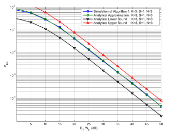
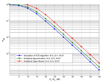
Figure 4: Comparison of the AOA/AOD probability of estimation error numerical results with the derived analytical expression. Fig. (a) uses shows the PEE for a single stage system, whereas Fig. (b) shows a system with S=3𝑆3S=3. Both systems use PR=1subscript𝑃𝑅1P_{R}=1 and are compared to the total energy per noise ratio, calculated by ET=Ms=1SPssubscript𝐸𝑇𝑀superscriptsubscript𝑠1𝑆subscript𝑃𝑠E_{T}=M\sum_{s=1}^{S}P_{s}. The Analytical Approximation, Lower Bound and Upper Bound in (a) refer to, (130), (131) and (121), respectively. In (b), the Analytical Approximation refers to the substitution of (130) into (133) where as the Analytical Upper Bound refers to the substitution of (121) into (133).

V-A Probability of AOD/AOA Estimation Error

As the RACE algorithm seeks to achieve a fixed error rate by means of an adaptive 𝑮(s,M+R)superscript𝑮𝑠𝑀𝑅\boldsymbol{G}^{(s,M+R)}, we first need to find the PEE for a fixed generator matrix, 𝑮(s,M+R),s=1,,Sformulae-sequencesuperscript𝑮𝑠𝑀𝑅for-all𝑠1𝑆\boldsymbol{G}^{(s,M+R)},\;\forall\;s=1,...,S. Note that this is also the case in Algorithm 1 with a fixed generator matrix, 𝑮(s,M),s=1,,Sformulae-sequencesuperscript𝑮𝑠𝑀for-all𝑠1𝑆\boldsymbol{G}^{(s,M)},\;\forall\;s=1,...,S. We begin by defining the PEE in a given stage s𝑠s, assuming all previous stages have been correct, as

pEE|𝑮(s,M+R),𝒗¯(s)=p(𝒗¯(s)𝒗^(s))subscript𝑝conditional𝐸𝐸superscript𝑮𝑠𝑀𝑅superscript¯𝒗𝑠𝑝superscript¯𝒗𝑠superscript^𝒗𝑠\displaystyle p_{EE|\boldsymbol{G}^{(s,M+R)},\bar{\boldsymbol{v}}^{(s)}}=p(\bar{\boldsymbol{v}}^{(s)}\neq\hat{\boldsymbol{v}}^{(s)}) (109)

where the term p(𝒗¯(s)𝒗^(s))𝑝superscript¯𝒗𝑠superscript^𝒗𝑠p(\bar{\boldsymbol{v}}^{(s)}\neq\hat{\boldsymbol{v}}^{(s)}) represents the probability that the estimated AOD/AOA information 𝒗^(s)superscript^𝒗𝑠\hat{\boldsymbol{v}}^{(s)} is not equal to the physical channel, 𝒗¯(s)superscript¯𝒗𝑠\bar{\boldsymbol{v}}^{(s)}.

If we treat the channel vector 𝒗¯(s)superscript¯𝒗𝑠\bar{\boldsymbol{v}}^{(s)} as information being encoded by the generator matrix 𝑮(s,M+R)superscript𝑮𝑠𝑀𝑅\boldsymbol{G}^{(s,M+R)}, we can model this estimation error event as a maximum likelihood decoding error. We can then say that 𝒗¯(s)𝒗^(s)superscript¯𝒗𝑠superscript^𝒗𝑠\bar{\boldsymbol{v}}^{(s)}\neq\hat{\boldsymbol{v}}^{(s)} occurs when the received measurement vector 𝒚(s)=αxPsN2Cs4𝑮(s,M+R)(𝒗¯(s))T+𝒏(s)superscript𝒚𝑠𝛼𝑥subscript𝑃𝑠superscript𝑁2superscriptsubscript𝐶𝑠4superscript𝑮𝑠𝑀𝑅superscriptsuperscript¯𝒗𝑠𝑇superscript𝒏𝑠\boldsymbol{y}^{(s)}=\alpha x\sqrt{P_{s}N^{2}C_{s}^{4}}\boldsymbol{G}^{(s,M+R)}(\bar{\boldsymbol{v}}^{(s)})^{T}+\boldsymbol{n}^{(s)}, is incorrectly ’decoded’ to another received measurement vector 𝒚(s)=αxPsN2Cs4𝑮(s,M+R)𝒗¯T,𝒗¯𝒱and𝒗¯𝒗¯(s)formulae-sequencesuperscript𝒚𝑠𝛼𝑥subscript𝑃𝑠superscript𝑁2superscriptsubscript𝐶𝑠4superscript𝑮𝑠𝑀𝑅superscript¯𝒗𝑇for-allsuperscript¯𝒗𝒱andsuperscript¯𝒗superscript¯𝒗𝑠\boldsymbol{y}^{\prime(s)}=\alpha x\sqrt{P_{s}N^{2}C_{s}^{4}}\boldsymbol{G}^{(s,M+R)}\bar{\boldsymbol{v}}^{\prime T},\;\forall\;\bar{\boldsymbol{v}}^{\prime}\in\mathcal{V}\;\text{and}\;\bar{\boldsymbol{v}}^{\prime}\neq\bar{\boldsymbol{v}}^{(s)}. We then express the probability of this event as

p(𝒗¯(s)𝒗^(s))=𝒗¯𝒱𝒗¯𝒗¯p(𝒚(s)𝒚(s)).𝑝superscript¯𝒗𝑠superscript^𝒗𝑠subscriptsuperscript¯𝒗𝒱superscript¯𝒗¯𝒗𝑝superscript𝒚𝑠superscript𝒚𝑠\displaystyle p(\bar{\boldsymbol{v}}^{(s)}\neq\hat{\boldsymbol{v}}^{(s)})=\bigcup\limits_{{\begin{array}[]{c}\bar{\boldsymbol{v}}^{\prime}\in\mathcal{V}\\ \bar{\boldsymbol{v}}^{\prime}\neq\bar{\boldsymbol{v}}\end{array}}}p(\boldsymbol{y}^{(s)}\rightarrow\boldsymbol{y}^{\prime(s)}). (112)

As the decoding approach used in this paper is based upon maximum likelihood, we can calculate such an error probability from the Euclidean distance between the received measurement sets. With reference to [36], we can then express the pairwise error probability of this decoding error over a fading channel with coefficient α𝒞𝒩(0,PR)similar-to𝛼𝒞𝒩0subscript𝑃𝑅\alpha\sim\mathcal{C}\mathcal{N}(0,P_{R}) as

p(𝒚(s)𝒚(s))𝑝superscript𝒚𝑠superscript𝒚𝑠\displaystyle p(\boldsymbol{y}^{(s)}\rightarrow\boldsymbol{y}^{\prime(s)}) =12[1γ¯2γ¯2+2]absent12delimited-[]1superscript¯𝛾2superscript¯𝛾22\displaystyle=\frac{1}{2}\Bigg{[}1-\sqrt{\frac{\bar{\gamma}^{2}}{\bar{\gamma}^{2}+2}}\Bigg{]} (113)

where

γ¯=PsCs4N2PR2N0𝑮(s,M+R)(𝒗¯(s)𝒗¯)T¯𝛾subscript𝑃𝑠superscriptsubscript𝐶𝑠4superscript𝑁2subscript𝑃𝑅2subscript𝑁0normsuperscript𝑮𝑠𝑀𝑅superscriptsuperscript¯𝒗𝑠superscript¯𝒗𝑇\displaystyle\bar{\gamma}=\sqrt{\frac{P_{s}C_{s}^{4}N^{2}P_{R}}{2N_{0}}}||{\boldsymbol{G}^{(s,M+R)}}(\bar{\boldsymbol{v}}^{(s)}-\bar{\boldsymbol{v}}^{\prime})^{T}|| (114)

By substituting these terms into (109) and averaging over each 𝒗¯(s)superscript¯𝒗𝑠\bar{\boldsymbol{v}}^{(s)} we get

pEE|𝑮(s,M+R)subscript𝑝conditional𝐸𝐸superscript𝑮𝑠𝑀𝑅\displaystyle p_{EE|\boldsymbol{G}^{(s,M+R)}} =𝒗¯𝒱p(𝒗¯)pEE|𝑮(s,M+R),𝒗¯(s)absentsubscript¯𝒗𝒱𝑝bold-¯𝒗subscript𝑝conditional𝐸𝐸superscript𝑮𝑠𝑀𝑅superscript¯𝒗𝑠\displaystyle=\sum\limits_{\bar{\boldsymbol{v}}\in\mathcal{V}}p(\boldsymbol{\bar{\boldsymbol{v}}})p_{EE|\boldsymbol{G}^{(s,M+R)},\bar{\boldsymbol{v}}^{(s)}} (115)
=𝒗¯𝒱𝒗¯𝒱𝒗¯𝒗¯p(𝒗¯)2[1γ¯2γ¯2+2].absentsubscript¯𝒗𝒱subscriptsuperscript¯𝒗𝒱superscript¯𝒗¯𝒗𝑝bold-¯𝒗2delimited-[]1superscript¯𝛾2superscript¯𝛾22\displaystyle=\sum\limits_{\bar{\boldsymbol{v}}\in\mathcal{V}}\bigcup\limits_{{\begin{array}[]{c}\bar{\boldsymbol{v}}^{\prime}\in\mathcal{V}\\ \bar{\boldsymbol{v}}^{\prime}\neq\bar{\boldsymbol{v}}\end{array}}}\frac{p(\boldsymbol{\bar{\boldsymbol{v}}})}{2}\Bigg{[}1-\sqrt{\frac{\bar{\gamma}^{2}}{\bar{\gamma}^{2}+2}}\Bigg{]}. (118)

Expressing the exact probability of the union term in (118) is quite difficult due to complicated boundaries between each column in 𝑮(s,M+R)superscript𝑮𝑠𝑀𝑅\boldsymbol{G}^{(s,M+R)}. This is a direct result of the generator matrix not containing a full set of normalized (M+R)×1𝑀𝑅1(M+R)\times 1 vectors. For example, (53) does not contain the scaled versions of the vectors [0,1,1,0]Tsuperscript0110𝑇[0,1,1,0]^{T} , [1,1,0,1]Tsuperscript1101𝑇[1,1,0,1]^{T}, [1,0,1,1]Tsuperscript1011𝑇[1,0,1,1]^{T}, [1,1,1,0]Tsuperscript1110𝑇[1,1,1,0]^{T}, [0,1,1,1]Tsuperscript0111𝑇[0,1,1,1]^{T} or [0,0,0,0]Tsuperscript0000𝑇[0,0,0,0]^{T}. This is an inherent property of the generator matrix being constructed from two smaller matrices 𝑩T(s,M)superscriptsubscript𝑩𝑇𝑠𝑀\boldsymbol{B}_{T}^{(s,M)} and 𝑩R(s,M)superscriptsubscript𝑩𝑅𝑠𝑀\boldsymbol{B}_{R}^{(s,M)} that do not contain the all-zero column vector. We can, however, find an upper bound of expression in (118) by replacing the union term with a summation to get

pEE|𝑮(s,M+R)<𝒗¯𝒱𝒗¯𝒱𝒗¯𝒗¯p(𝒗¯)2[1γ¯2γ¯2+2].subscript𝑝conditional𝐸𝐸superscript𝑮𝑠𝑀𝑅subscript¯𝒗𝒱subscriptsuperscript¯𝒗𝒱superscript¯𝒗¯𝒗𝑝bold-¯𝒗2delimited-[]1superscript¯𝛾2superscript¯𝛾22\displaystyle p_{EE|\boldsymbol{G}^{(s,M+R)}}<\sum\limits_{\bar{\boldsymbol{v}}\in\mathcal{V}}\sum\limits_{{\begin{array}[]{c}\bar{\boldsymbol{v}}^{\prime}\in\mathcal{V}\\ \bar{\boldsymbol{v}}^{\prime}\neq\bar{\boldsymbol{v}}\end{array}}}\frac{p(\boldsymbol{\bar{\boldsymbol{v}}})}{2}\Bigg{[}1-\sqrt{\frac{\bar{\gamma}^{2}}{\bar{\gamma}^{2}+2}}\Bigg{]}. (121)

The resulting upper bound in (121) is found to be quite loose in most cases. Motivated by this, we find a much tighter approximation by only considering 𝒗¯superscript¯𝒗\bar{\boldsymbol{v}}^{\prime} that minimizes 𝑮(s,M+R)(𝒗¯(s)𝒗¯)Tnormsuperscript𝑮𝑠𝑀𝑅superscriptsuperscript¯𝒗𝑠superscript¯𝒗𝑇||{\boldsymbol{G}^{(s,M+R)}}(\bar{\boldsymbol{v}}^{(s)}-\bar{\boldsymbol{v}}^{\prime})^{T}|| (i.e., only considering spatially adjacent columns of 𝑮(s,M+R)superscript𝑮𝑠𝑀𝑅\boldsymbol{G}^{(s,M+R)}). We define this minimum distance for each 𝒗¯(s)superscript¯𝒗𝑠\bar{\boldsymbol{v}}^{(s)} by

dmin(𝒗¯(s))=min𝒗¯𝒱𝒗¯𝒗¯𝑮(s,M+R)(𝒗¯(s)𝒗¯)Tsubscript𝑑𝑚𝑖𝑛superscript¯𝒗𝑠superscript¯𝒗𝒱superscript¯𝒗¯𝒗minnormsuperscript𝑮𝑠𝑀𝑅superscriptsuperscript¯𝒗𝑠superscript¯𝒗𝑇\displaystyle d_{min}(\bar{\boldsymbol{v}}^{(s)})=\underset{{\begin{array}[]{c}\bar{\boldsymbol{v}}^{\prime}\in\mathcal{V}\\ \bar{\boldsymbol{v}}^{\prime}\neq\bar{\boldsymbol{v}}\end{array}}}{\operatorname{min}}||{\boldsymbol{G}^{(s,M+R)}}(\bar{\boldsymbol{v}}^{(s)}-\bar{\boldsymbol{v}}^{\prime})^{T}|| (124)

and the set of vectors causing it as

𝒱min(𝒗¯(s))={argmin𝒗¯𝒱min𝒗¯𝒗¯𝑮(s,M+R)(𝒗¯(s)𝒗¯)T}.subscript𝒱𝑚𝑖𝑛superscript¯𝒗𝑠superscript¯𝒗subscript𝒱𝑚𝑖𝑛superscript¯𝒗¯𝒗argminnormsuperscript𝑮𝑠𝑀𝑅superscriptsuperscript¯𝒗𝑠superscript¯𝒗𝑇\displaystyle\mathcal{V}_{min}(\bar{\boldsymbol{v}}^{(s)})=\Big{\{}\underset{{\begin{array}[]{c}\bar{\boldsymbol{v}}^{\prime}\in\mathcal{V}_{min}\\ \bar{\boldsymbol{v}}^{\prime}\neq\bar{\boldsymbol{v}}\end{array}}}{\operatorname{argmin}}||{\boldsymbol{G}^{(s,M+R)}}(\bar{\boldsymbol{v}}^{(s)}-\bar{\boldsymbol{v}}^{\prime})^{T}||\Big{\}}. (127)

We therefore approximate pEE|𝑮(s,M+R)subscript𝑝conditional𝐸𝐸superscript𝑮𝑠𝑀𝑅p_{EE|\boldsymbol{G}^{(s,M+R)}} by

pEE|𝑮(s,M+R)𝒗¯𝒱𝒗¯𝒱min𝒗¯𝒗¯p(𝒗¯)2[1γ¯2γ¯2+2].subscript𝑝conditional𝐸𝐸superscript𝑮𝑠𝑀𝑅subscript¯𝒗𝒱subscriptsuperscript¯𝒗subscript𝒱𝑚𝑖𝑛superscript¯𝒗¯𝒗𝑝bold-¯𝒗2delimited-[]1superscript¯𝛾2superscript¯𝛾22\displaystyle p_{EE|\boldsymbol{G}^{(s,M+R)}}\approx\;\sum\limits_{\bar{\boldsymbol{v}}\in\mathcal{V}}\sum\limits_{{\begin{array}[]{c}\bar{\boldsymbol{v}}^{\prime}\in\mathcal{V}_{min}\\ \bar{\boldsymbol{v}}^{\prime}\neq\bar{\boldsymbol{v}}\end{array}}}\frac{p(\boldsymbol{\bar{\boldsymbol{v}}})}{2}\Bigg{[}1-\sqrt{\frac{\bar{\gamma}^{2}}{\bar{\gamma}^{2}+2}}\Bigg{]}. (130)

We also provide a greatly simplified lower bound for Algorithm 1 when R=0𝑅0R=0, by only considering a single one of these 𝒗¯superscript¯𝒗\bar{\boldsymbol{v}}^{\prime} that cause a minimum distance. Recall that the generator matrix is designed such that all paths have the same minimum Euclidean distance, which we define here as Emin=dmin(𝒗¯(s)),𝒗¯(s)subscript𝐸𝑚𝑖𝑛subscript𝑑𝑚𝑖𝑛superscript¯𝒗𝑠for-allsuperscript¯𝒗𝑠\sqrt{E_{min}}=d_{min}(\bar{\boldsymbol{v}}^{(s)}),\;\forall\;\bar{\boldsymbol{v}}^{(s)}. By assuming each channel realization is equiprobable, this leads to

pEE|𝑮(s,M)>12[1PsCs4N2PREminPsCs4N2PREmin+4N0]subscript𝑝conditional𝐸𝐸superscript𝑮𝑠𝑀12delimited-[]1subscript𝑃𝑠superscriptsubscript𝐶𝑠4superscript𝑁2subscript𝑃𝑅subscript𝐸𝑚𝑖𝑛subscript𝑃𝑠superscriptsubscript𝐶𝑠4superscript𝑁2subscript𝑃𝑅subscript𝐸𝑚𝑖𝑛4subscript𝑁0\displaystyle p_{EE|\boldsymbol{G}^{(s,M)}}>\frac{1}{2}\Bigg{[}1-\sqrt{\frac{{{P_{s}C_{s}^{4}N^{2}P_{R}{E_{min}}}}}{{{P_{s}C_{s}^{4}N^{2}P_{R}{E_{min}}}}+4N_{0}}}\;\Bigg{]} (131)

Finally, we upper bound the probability of an error occurring in any of the S𝑆S stages as

pEEsubscript𝑝𝐸𝐸\displaystyle p_{EE} =1s=1S(1pEE|𝑮(s,M+R))absent1superscriptsubscriptproduct𝑠1𝑆1subscript𝑝conditional𝐸𝐸superscript𝑮𝑠𝑀𝑅\displaystyle=1-\prod\limits_{s=1}^{S}(1-p_{EE|\boldsymbol{G}^{(s,M+R)}}) (132)
<s=1SpEE|𝑮(s,M+R)absentsuperscriptsubscript𝑠1𝑆subscript𝑝conditional𝐸𝐸superscript𝑮𝑠𝑀𝑅\displaystyle<\;\sum\limits_{s=1}^{S}p_{EE|\boldsymbol{G}^{(s,M+R)}} (133)
<s=1S𝒗¯𝒱𝒗¯𝒱𝒗¯𝒗¯(s)p(𝒗¯)2[1γ¯2γ¯2+2].absentsuperscriptsubscript𝑠1𝑆subscript¯𝒗𝒱subscriptsuperscript¯𝒗𝒱superscript¯𝒗superscript¯𝒗𝑠𝑝bold-¯𝒗2delimited-[]1superscript¯𝛾2superscript¯𝛾22\displaystyle<\;\sum\limits_{s=1}^{S}\sum\limits_{\bar{\boldsymbol{v}}\in\mathcal{V}}\sum\limits_{{\begin{array}[]{c}\bar{\boldsymbol{v}}^{\prime}\in\mathcal{V}\\ \bar{\boldsymbol{v}}^{\prime}\neq\bar{\boldsymbol{v}}^{(s)}\end{array}}}\frac{p(\boldsymbol{\bar{\boldsymbol{v}}})}{2}\Bigg{[}1-\sqrt{\frac{\bar{\gamma}^{2}}{\bar{\gamma}^{2}+2}}\Bigg{]}. (136)

In order to validate our analysis, Figs. 4 (a) and (b) compare the derived analytical expressions with their corresponding Monte Carlo simulations for a single stage system and three stage system, respectively. As we can observe from Fig. 4(a), the given in (130) is actually quite tight. Focusing on the three stage system in Fig. 4(b), we see that the substitution of the approximation in (130) into the upper bound (133) causes some disparity, however still provides a tighter approximation than (136). A lower bound is not presented in Fig. 4(b) as the use of (131) in the upper bound (133) would not be mathematically correct.

V-B Minimum Energy and Time Requirement for the RACE Algorithm

We now present an expression for the minimum signal energy-to-noise ratio required by the RACE algorithm for an average number of measurements in a given stage. From an information theory standpoint, we can describe the RACE algorithm as the information process that a 1×K21superscript𝐾21\times K^{2} binary vector 𝒗¯(s)superscript¯𝒗𝑠\bar{\boldsymbol{v}}^{(s)} is encoded into M+R𝑀𝑅M+R symbols by the generator matrix 𝑮(s,M+R)superscript𝑮𝑠𝑀𝑅\boldsymbol{G}^{(s,M+R)}. This information transfer has an equivalent modulation rate of C=K2/(M+R)𝐶superscript𝐾2𝑀𝑅C=K^{2}/(M+R) information bits per measurement time slot duration. The Shannon-Hartley theorem [37] tells us that the minimum received SNR required for error free detection at this rate is

SNRr𝑆𝑁subscript𝑅𝑟\displaystyle SNR_{r} 2C1absentsuperscript2𝐶1\displaystyle\geq 2^{C}-1
=2K2M+R1absentsuperscript2superscript𝐾2𝑀𝑅1\displaystyle=2^{\frac{K^{2}}{M+R}}-1 (137)

where from (77), for a given 𝒗¯(s)superscript¯𝒗𝑠\bar{\boldsymbol{v}}^{(s)}, 𝑮(s,M+R)superscript𝑮𝑠𝑀𝑅\boldsymbol{G}^{(s,M+R)} and α𝛼\alpha, we know the average received SNR can be expressed as

SNRr=α2PsCs4N2N0𝑮(s,M+R)(𝒗¯(s))T2(M+R).𝑆𝑁subscript𝑅𝑟superscriptnorm𝛼2subscript𝑃𝑠superscriptsubscript𝐶𝑠4superscript𝑁2subscript𝑁0superscriptnormsuperscript𝑮𝑠𝑀𝑅superscriptsuperscript¯𝒗𝑠𝑇2𝑀𝑅\displaystyle SNR_{r}=\frac{||\alpha||^{2}P_{s}C_{s}^{4}N^{2}}{N_{0}}\frac{||\boldsymbol{G}^{(s,M+R)}(\bar{\boldsymbol{v}}^{(s)})^{T}||^{2}}{(M+R)}. (138)

Substituting (138) into (V-B) gives

α2PsCs4N2N0𝑮(s,M+R)(𝒗¯(s))T2(M+R)2K2(M+R)1.superscriptnorm𝛼2subscript𝑃𝑠superscriptsubscript𝐶𝑠4superscript𝑁2subscript𝑁0superscriptnormsuperscript𝑮𝑠𝑀𝑅superscriptsuperscript¯𝒗𝑠𝑇2𝑀𝑅superscript2superscript𝐾2𝑀𝑅1\displaystyle\frac{||\alpha||^{2}P_{s}C_{s}^{4}N^{2}}{N_{0}}\frac{||\boldsymbol{G}^{(s,M+R)}(\bar{\boldsymbol{v}}^{(s)})^{T}||^{2}}{(M+R)}\geq 2^{\frac{K^{2}}{(M+R)}}-1. (139)

By denoting the total energy used in stage s𝑠s by Es=Ps(M+R)subscript𝐸𝑠subscript𝑃𝑠𝑀𝑅E_{s}=P_{s}(M+R), we can re-write (139) as

EsN0(M+R)2(2K2(M+R)1)α2Cs4N2𝑮(s,M+R)(𝒗¯(s))T2.subscript𝐸𝑠subscript𝑁0superscript𝑀𝑅2superscript2superscript𝐾2𝑀𝑅1superscriptnorm𝛼2superscriptsubscript𝐶𝑠4superscript𝑁2superscriptnormsuperscript𝑮𝑠𝑀𝑅superscriptsuperscript¯𝒗𝑠𝑇2\displaystyle\frac{E_{s}}{N_{0}}\geq\frac{(M+R)^{2}(2^{\frac{K^{2}}{(M+R)}}-1)}{||\alpha||^{2}C_{s}^{4}N^{2}||\boldsymbol{G}^{(s,M+R)}(\bar{\boldsymbol{v}}^{(s)})^{T}||^{2}}. (140)
Refer to caption
Figure 5: Comparison of the minimum number of measurements required for channel estimation in a single stage, using the RACE algorithm, to the analytical expression in (144) with pFB=1subscript𝑝𝐹𝐵1p_{FB}=1 and pFB=1/K2subscript𝑝𝐹𝐵1superscript𝐾2p_{FB}=1/K^{2}. Here we use N=3𝑁3N=3, K=3𝐾3K=3, α=1norm𝛼1||\alpha||=1 and Mmax=subscript𝑀𝑚𝑎𝑥M_{max}=\infty.

The expression in (140) gives a good insight into how to minimize the amount of energy required for successful channel estimation. For example, one intuitive approach to reduce the energy requirement is to maximize the term, Cs4N2𝑮(s,M+R)(𝒗¯(s))T2subscriptsuperscript𝐶4𝑠superscript𝑁2superscriptnormsuperscript𝑮𝑠𝑀𝑅superscriptsuperscript¯𝒗𝑠𝑇2C^{4}_{s}N^{2}||\boldsymbol{G}^{(s,M+R)}(\bar{\boldsymbol{v}}^{(s)})^{T}||^{2} which directly determines the amount of energy that arrives at the receiver. Furthermore, as we have a minimum number of M𝑀M initial measurements that have been designed such that they propagate non-zero energy over each sub-range combination (i.e., each column of 𝑮(s,M+R)superscript𝑮𝑠𝑀𝑅\boldsymbol{G}^{(s,M+R)} has a non-zero norm), we ensure that 𝑮(s,M+R)(𝒗¯(s))T2>0,𝒗¯(s)superscriptnormsuperscript𝑮𝑠𝑀𝑅superscriptsuperscript¯𝒗𝑠𝑇20for-allsuperscript¯𝒗𝑠||\boldsymbol{G}^{(s,M+R)}(\bar{\boldsymbol{v}}^{(s)})^{T}||^{2}>0,\;\forall\;\bar{\boldsymbol{v}}^{(s)}. This then guarantees that Es/N0subscript𝐸𝑠subscript𝑁0E_{s}/N_{0} always takes on a finite value.

As 𝑮(s,M+R)superscript𝑮𝑠𝑀𝑅\boldsymbol{G}^{(s,M+R)} is adaptive and based on feedback, it becomes quite difficult to determine the exact energy requirement for various R>0𝑅0R>0. However, if we let 𝒈t(s,M+R)subscriptsuperscript𝒈𝑠𝑀𝑅𝑡\boldsymbol{g}^{(s,M+R)}_{t} denote the t𝑡tth row of 𝑮(s,M+R)superscript𝑮𝑠𝑀𝑅\boldsymbol{G}^{(s,M+R)}, we can expand the term 𝑮(s,M+R)(𝒗¯(s))T2superscriptnormsuperscript𝑮𝑠𝑀𝑅superscriptsuperscript¯𝒗𝑠𝑇2||\boldsymbol{G}^{(s,M+R)}(\bar{\boldsymbol{v}}^{(s)})^{T}||^{2} by splitting it into the sum of received energy in each measurement time slots. The row/column energy normalization, seen in the design of (42), leads to the generator matrix having 𝑮(s,M)(𝒗¯(s))T2=MK2𝒗¯(s)superscriptnormsuperscript𝑮𝑠𝑀superscriptsuperscript¯𝒗𝑠𝑇2𝑀superscript𝐾2for-allsuperscript¯𝒗𝑠||\boldsymbol{G}^{(s,M)}(\bar{\boldsymbol{v}}^{(s)})^{T}||^{2}=\frac{M}{K^{2}}\;\forall\;\bar{\boldsymbol{v}}^{(s)}. Expanding this expression we then get

𝑮(s,M+R)(𝒗¯(s))T2superscriptnormsuperscript𝑮𝑠𝑀𝑅superscriptsuperscript¯𝒗𝑠𝑇2\displaystyle||\boldsymbol{G}^{(s,M+R)}(\bar{\boldsymbol{v}}^{(s)})^{T}||^{2}
=t=1M+R(𝒈t(s,M+R)(𝒗¯(s))T)2absentsuperscriptsubscript𝑡1𝑀𝑅superscriptsubscriptsuperscript𝒈𝑠𝑀𝑅𝑡superscriptsuperscript¯𝒗𝑠𝑇2\displaystyle=\sum\limits_{t=1}^{M+R}\big{(}\boldsymbol{g}^{(s,M+R)}_{t}(\bar{\boldsymbol{v}}^{(s)})^{T}\big{)}^{2}
=𝑮(s,M)(𝒗¯(s))T2+t=M+1M+R(𝒈t(s,M+R)(𝒗¯(s))T)2absentsuperscriptnormsuperscript𝑮𝑠𝑀superscriptsuperscript¯𝒗𝑠𝑇2superscriptsubscript𝑡𝑀1𝑀𝑅superscriptsubscriptsuperscript𝒈𝑠𝑀𝑅𝑡superscriptsuperscript¯𝒗𝑠𝑇2\displaystyle=||\boldsymbol{G}^{(s,M)}(\bar{\boldsymbol{v}}^{(s)})^{T}||^{2}+\sum\limits_{t=M+1}^{M+R}\big{(}\boldsymbol{g}^{(s,M+R)}_{t}(\bar{\boldsymbol{v}}^{(s)})^{T}\big{)}^{2}
=MK2+t=M+1M+R(𝒈t(s,M+R)(𝒗¯(s))T)2.absent𝑀superscript𝐾2superscriptsubscript𝑡𝑀1𝑀𝑅superscriptsubscriptsuperscript𝒈𝑠𝑀𝑅𝑡superscriptsuperscript¯𝒗𝑠𝑇2\displaystyle=\frac{M}{K^{2}}+\sum\limits_{t=M+1}^{M+R}\big{(}\boldsymbol{g}^{(s,M+R)}_{t}(\bar{\boldsymbol{v}}^{(s)})^{T}\big{)}^{2}. (141)

Following the RACE algorithm, we can also deduce that the term 𝒈t(s,M+R)(𝒗¯(s))Tsubscriptsuperscript𝒈𝑠𝑀𝑅𝑡superscriptsuperscript¯𝒗𝑠𝑇\boldsymbol{g}^{(s,M+R)}_{t}(\bar{\boldsymbol{v}}^{(s)})^{T} in (V-B) results in either unit energy or no energy, depending on whether the most likely sub-range combination from the previous measurement timeslot was correct or not. If we denote the probability of this information being incorrect as pEE|𝑮(s,M+R1)subscript𝑝conditional𝐸𝐸superscript𝑮𝑠𝑀𝑅1p_{EE|\boldsymbol{G}^{(s,M+R-1)}} we can then write the average energy contribution from this term as

𝑮(s,M+R)(𝒗¯(s))T2=MK2+R=1R(1pEE|𝑮(s,M+R1)).superscriptnormsuperscript𝑮𝑠𝑀𝑅superscriptsuperscript¯𝒗𝑠𝑇2𝑀superscript𝐾2superscriptsubscriptsuperscript𝑅1𝑅1subscript𝑝conditional𝐸𝐸superscript𝑮𝑠𝑀superscript𝑅1\displaystyle||\boldsymbol{G}^{(s,M+R)}(\bar{\boldsymbol{v}}^{(s)})^{T}||^{2}=\frac{M}{K^{2}}+\sum\limits_{R^{\prime}=1}^{R}(1-p_{EE|\boldsymbol{G}^{(s,M+R^{\prime}-1)}}). (142)

Substituting (142) back into (140), we have

EsN0(M+R)2(2K2M+R1)Cs4N2α2[MK2+R=1R(1pEE|𝑮(s,M+R1))].subscript𝐸𝑠subscript𝑁0superscript𝑀𝑅2superscript2superscript𝐾2𝑀𝑅1superscriptsubscript𝐶𝑠4superscript𝑁2superscriptnorm𝛼2delimited-[]𝑀superscript𝐾2superscriptsubscriptsuperscript𝑅1𝑅1subscript𝑝conditional𝐸𝐸superscript𝑮𝑠𝑀superscript𝑅1\displaystyle\frac{E_{s}}{N_{0}}\geq\frac{(M+R)^{2}(2^{\frac{K^{2}}{M+R}}-1)}{C_{s}^{4}N^{2}||\alpha||^{2}\Big{[}\frac{M}{K^{2}}+\sum\limits_{R^{\prime}=1}^{R}(1-p_{EE|\boldsymbol{G}^{(s,M+R^{\prime}-1)}})\Big{]}}. (143)

Unfortunately, the probability in (143) still depends on previous sub-range estimates determined from the previous measurement and is thus difficult to obtain a closed-form. We can however, consider a few extreme cases where we assume a fixed probability of correct feedback information. That is, we use pFB=1pEE|𝑮(s,M+R1),R>0formulae-sequencesubscript𝑝𝐹𝐵1subscript𝑝conditional𝐸𝐸superscript𝑮𝑠𝑀𝑅1for-all𝑅0p_{FB}=1-p_{EE|\boldsymbol{G}^{(s,M+R-1)}},\;\forall\;R>0. Finally, we can express the average minimum energy to noise ratio required for successful channel estimation in a given stage with a certain number of measurements to be

EsN0(M+R)2(2K2M+R1)Cs4N2α2[MK2+R×pFB].subscript𝐸𝑠subscript𝑁0superscript𝑀𝑅2superscript2superscript𝐾2𝑀𝑅1superscriptsubscript𝐶𝑠4superscript𝑁2superscriptnorm𝛼2delimited-[]𝑀superscript𝐾2𝑅subscript𝑝𝐹𝐵\displaystyle\frac{E_{s}}{N_{0}}\geq\frac{(M+R)^{2}(2^{\frac{K^{2}}{M+R}}-1)}{C_{s}^{4}N^{2}||\alpha||^{2}\Big{[}\frac{M}{K^{2}}+R\times p_{FB}\Big{]}}. (144)

To validate this expression, Fig. 5 shows the average number of measurements required to estimate the AOD/AOA information in a single stage for a range of different signal energy to noise ratios. Here we also plot (144) for two special cases. The first is when pFB=1subscript𝑝𝐹𝐵1p_{FB}=1, representing the best case scenario where the previous sub-range estimate is always correct. The second is the worst case scenario where the previous sub-range estimate is random (i.e., no feedback) giving pFB=1/K2subscript𝑝𝐹𝐵1superscript𝐾2p_{FB}=1/K^{2}.

As we can see from Fig. 5, (144) provides a bound for the best case scenario pFB=1subscript𝑝𝐹𝐵1p_{FB}=1, and for the worst case scenario pFB=1/K2subscript𝑝𝐹𝐵1superscript𝐾2p_{FB}=1/K^{2}. To make the simulation results match the bounds, here we do not limit the number of measurements (i.e., Mmax=subscript𝑀𝑚𝑎𝑥M_{max}=\infty). Although pFB=1/K2subscript𝑝𝐹𝐵1superscript𝐾2p_{FB}=1/K^{2} still gives a mathematical lower bound for the energy requirement, the condition that pFB=1/K2subscript𝑝𝐹𝐵1superscript𝐾2p_{FB}=1/K^{2} describes a system that performs far worse than the RACE algorithm. As such, we see the two lines intercept at high SNR. We can also observe from this figure that the RACE algorithm falls between these two curves and converges to R=0𝑅0R=0 at high SNR. Finally, the asymptotic nature of the results in Fig. 5 supports the need to set Mmax<<much-less-thansubscript𝑀𝑚𝑎𝑥M_{max}<<\infty so that measurements do not continue indefinitely.

V-C Discussion of System Performance Parameters
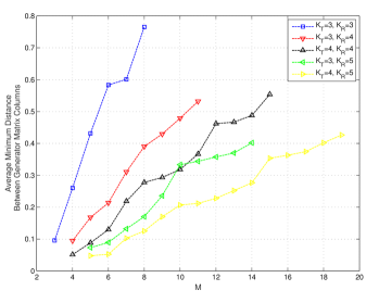
Refer to caption
Figure 6: Average minimum distance between the columns of the optimized generator matrix versus the number of measurements, M𝑀M, for a range of different sized beam pattern description matrices.

We end this section by briefly discussing the performance parameter selection for the proposed algorithms for a generalized mmWave MIMO system with Ntsubscript𝑁𝑡N_{t} transmit antenna and Nrsubscript𝑁𝑟N_{r} receive antenna, each equipped with a limited number of RF chains such that they can only transmit and receive with a single beam pattern.

V-C1 Selection of number of sub-ranges in each stage, K𝐾K

In general, by using a smaller value of K𝐾K, a faster channel estimation can be achieved at a greater energy efficiency and a more computationally efficient ML detection. The main drawback of setting a smaller K𝐾K lies in the wider beam patterns and the resultant loss of directionality gain. From an energy efficiency point of view, this loss is outweighed by the speed advantage. However, if a peak power constraint were imposed, more directionality may be required in the early stages and this can be achieved by increasing K𝐾K. Selection of K𝐾K may also depend on the number of antennas being equipped at each link end. For example, it is generally accepted that a mmWave mobile link will have more antennas at a base station (BS) than at the mobile station (MS) [38, 6]. For such a general asymmetric system, it is possible to use different K𝐾K in each stage and at each transceiver end. This grants flexibility to achieve the same number of estimation stages for each system. Then it is only important that the product of the K𝐾K’s over all stages equals to the antenna number. An alternative approach is to simply use more stages at the BS than at the MS. In this case, once the MS has reached its final stage before the transmitter, it can continue its role in the estimation procedure by utilizing the already estimated AOA.

V-C2 Selection of M𝑀M and design of 𝑩T(s,M)superscriptsubscript𝑩𝑇𝑠𝑀\boldsymbol{B}_{T}^{(s,M)} and 𝑩R(s,M)superscriptsubscript𝑩𝑅𝑠𝑀\boldsymbol{B}_{R}^{(s,M)}

Given that K𝐾K in each stage has been selected for an arbitrary antenna number N𝑁N, we now propose a method to find the optimal design of the beam pattern description matrices 𝑩T(s,M)superscriptsubscript𝑩𝑇𝑠𝑀\boldsymbol{B}_{T}^{(s,M)} and 𝑩R(s,M)superscriptsubscript𝑩𝑅𝑠𝑀\boldsymbol{B}_{R}^{(s,M)}. To include the asymmetric case where K𝐾K is different at the transmitter and receiver, we use KTsubscript𝐾𝑇K_{T} and KRsubscript𝐾𝑅K_{R} to denote the number of sub-ranges at the transmitter and receiver, respectively. We therefore find the optimal design of 𝑩T(s,M)superscriptsubscript𝑩𝑇𝑠𝑀\boldsymbol{B}_{T}^{(s,M)} and 𝑩R(s,M)superscriptsubscript𝑩𝑅𝑠𝑀\boldsymbol{B}_{R}^{(s,M)} for an arbitrary KTsubscript𝐾𝑇K_{T}, KRsubscript𝐾𝑅K_{R} and M𝑀M based on the theoretical analysis of PEE conducted in the previous sub-sections. With this result, we then show the performance trade-off for selecting larger/smaller M.

From the analytical expressions (109)-(114), we can see that minimizing the PEE is equivalent to maximizing the expression in (114). We denote the optimal beam pattern description matrices by 𝑩Topt(s,M)superscriptsubscript𝑩subscript𝑇𝑜𝑝𝑡𝑠𝑀\boldsymbol{B}_{T_{opt}}^{(s,M)} and 𝑩Ropt(s,M)superscriptsubscript𝑩subscript𝑅𝑜𝑝𝑡𝑠𝑀\boldsymbol{B}_{R_{opt}}^{(s,M)} at the transmitter and receiver, respectively, and we thus have

{𝑩Topt(s,M),𝑩Ropt(s,M)}=superscriptsubscript𝑩subscript𝑇𝑜𝑝𝑡𝑠𝑀superscriptsubscript𝑩subscript𝑅𝑜𝑝𝑡𝑠𝑀absent\displaystyle\{\boldsymbol{B}_{T_{opt}}^{(s,M)},\boldsymbol{B}_{R_{opt}}^{(s,M)}\}=
argmax𝑩T,𝑩RPsCs4N2PR2N0𝑮(s,M)(𝒗¯(s)𝒗¯)T,subscript𝑩𝑇subscript𝑩𝑅argmaxsubscript𝑃𝑠superscriptsubscript𝐶𝑠4superscript𝑁2subscript𝑃𝑅2subscript𝑁0normsuperscript𝑮𝑠𝑀superscriptsuperscript¯𝒗𝑠superscript¯𝒗𝑇\displaystyle\;\;\;\;\;\ \underset{{\boldsymbol{B}_{T}},\boldsymbol{B}_{R}}{\operatorname{argmax}}\sqrt{\frac{P_{s}C_{s}^{4}N^{2}P_{R}}{2N_{0}}}||{\boldsymbol{G}^{(s,M)}}(\bar{\boldsymbol{v}}^{(s)}-\bar{\boldsymbol{v}}^{\prime})^{T}||,
s.t., diag(𝑩T(𝑩T)H)=𝟏,diag(𝑩R(𝑩R)H)=𝟏,formulae-sequences.t., diagsubscript𝑩𝑇superscriptsubscript𝑩𝑇𝐻1diagsubscript𝑩𝑅superscriptsubscript𝑩𝑅𝐻1\displaystyle\text{s.t., }\text{diag}(\boldsymbol{B}_{T}(\boldsymbol{B}_{T})^{H})=\boldsymbol{1},\text{diag}(\boldsymbol{B}_{R}(\boldsymbol{B}_{R})^{H})=\boldsymbol{1},
diag((𝑩T)H𝑩T)=MK𝟏,diag((𝑩R)H𝑩R)=MK𝟏formulae-sequencediagsuperscriptsubscript𝑩𝑇𝐻subscript𝑩𝑇𝑀𝐾1diagsuperscriptsubscript𝑩𝑅𝐻subscript𝑩𝑅𝑀𝐾1\displaystyle\text{diag}((\boldsymbol{B}_{T})^{H}\boldsymbol{B}_{T})=\frac{M}{K}\boldsymbol{1},\text{diag}((\boldsymbol{B}_{R})^{H}\boldsymbol{B}_{R})=\frac{M}{K}\boldsymbol{1} (145)

by recalling that 𝑮(s,M)=𝑩T(s,M)𝑩R(s,M)superscript𝑮𝑠𝑀direct-productsuperscriptsubscript𝑩𝑇𝑠𝑀superscriptsubscript𝑩𝑅𝑠𝑀\boldsymbol{G}^{(s,M)}=\boldsymbol{B}_{T}^{(s,M)}\odot\boldsymbol{B}_{R}^{(s,M)} and where 𝟏1\boldsymbol{1} is an all-1 vector. The constraints imposed on 𝑩T(s,M)superscriptsubscript𝑩𝑇𝑠𝑀\boldsymbol{B}_{T}^{(s,M)} and 𝑩R(s,M)superscriptsubscript𝑩𝑅𝑠𝑀\boldsymbol{B}_{R}^{(s,M)} in (V-C2-V-C2), correspond the rows and columns of the matrices having a constant norm. To avoid repetition, we do not list the constraints under (146-V-C2), however they still apply. The row and column normalization are imposed, respectively, to:
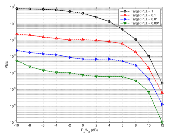
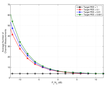
Refer to caption
Refer to caption
Figure 7: (a) Probability of estimation error (PEE) results of the RACE algorithm and (b) average number of measurements over a single path AWGN channel with varying target PEE, ΓΓ\Gamma
  1. 1.

    Keep a constant transmit power for each measurement of a given stage. It can be achieved when the norms of all rows in 𝑩T(s,M)superscriptsubscript𝑩𝑇𝑠𝑀\boldsymbol{B}_{T}^{(s,M)} are the same i.e., diag(𝑩T(𝑩T)H)=𝟏diagsubscript𝑩𝑇superscriptsubscript𝑩𝑇𝐻1\text{diag}(\boldsymbol{B}_{T}(\boldsymbol{B}_{T})^{H})=\boldsymbol{1}. Similarly, to receive with unit gain, we also have and diag((𝑩R)H𝑩R)=MK𝟏diagsuperscriptsubscript𝑩𝑅𝐻subscript𝑩𝑅𝑀𝐾1\text{diag}((\boldsymbol{B}_{R})^{H}\boldsymbol{B}_{R})=\frac{M}{K}\boldsymbol{1}.

  2. 2.

    Keep the total energy collected by different AOD/AOA sub-range combinations across all the measurements the same. This ensures the fairness of estimation success in all sub-range combinations. It can be achieved when the norms of all columns in 𝑩T(s,M)superscriptsubscript𝑩𝑇𝑠𝑀\boldsymbol{B}_{T}^{(s,M)} and 𝑩R(s,M)superscriptsubscript𝑩𝑅𝑠𝑀\boldsymbol{B}_{R}^{(s,M)} are the same, e.g., diag((𝑩T)H)𝑩T=MK𝟏,diag((𝑩R)H𝑩R)=MK𝟏formulae-sequencediagsuperscriptsubscript𝑩𝑇𝐻subscript𝑩𝑇𝑀𝐾1diagsuperscriptsubscript𝑩𝑅𝐻subscript𝑩𝑅𝑀𝐾1\text{diag}((\boldsymbol{B}_{T})^{H})\boldsymbol{B}_{T}=\frac{M}{K}\boldsymbol{1},\text{diag}((\boldsymbol{B}_{R})^{H}\boldsymbol{B}_{R})=\frac{M}{K}\boldsymbol{1}.

Since the square root term is independent of 𝑩T(s,M)superscriptsubscript𝑩𝑇𝑠𝑀\boldsymbol{B}_{T}^{(s,M)} and 𝑩R(s,M)superscriptsubscript𝑩𝑅𝑠𝑀\boldsymbol{B}_{R}^{(s,M)} for a fixed KTsubscript𝐾𝑇K_{T} and KRsubscript𝐾𝑅K_{R}, we thus can rewrite (V-C2) as

{𝑩Topt(s,M),𝑩Ropt(s,M)}=argmax𝑩T,𝑩R𝑮(s,M)(𝒗¯(s)𝒗¯)T.superscriptsubscript𝑩subscript𝑇𝑜𝑝𝑡𝑠𝑀superscriptsubscript𝑩subscript𝑅𝑜𝑝𝑡𝑠𝑀subscript𝑩𝑇subscript𝑩𝑅argmaxnormsuperscript𝑮𝑠𝑀superscriptsuperscript¯𝒗𝑠superscript¯𝒗𝑇\displaystyle\{\boldsymbol{B}_{T_{opt}}^{(s,M)},\boldsymbol{B}_{R_{opt}}^{(s,M)}\}=\underset{{\boldsymbol{B}_{T},\boldsymbol{B}_{R}}}{\operatorname{argmax}}||{\boldsymbol{G}^{(s,M)}}(\bar{\boldsymbol{v}}^{(s)}-\bar{\boldsymbol{v}}^{\prime})^{T}||. (146)

For channels with a single dominant path, the vectors 𝒗(s)superscript𝒗𝑠\boldsymbol{v}^{(s)} and 𝒗superscript𝒗\boldsymbol{v}^{\prime} only contain a single non-zero element. More specifically, 𝑮(s,M)(𝒗(s)𝒗)superscript𝑮𝑠𝑀superscript𝒗𝑠superscript𝒗\boldsymbol{G}^{(s,M)}(\boldsymbol{v}^{(s)}-\boldsymbol{v}^{\prime}) can be simplified to the subtraction of two columns of 𝑮(s,M)superscript𝑮𝑠𝑀\boldsymbol{G}^{(s,M)}. Since the channel estimation error is dominated by the columns of 𝑮(s,M)superscript𝑮𝑠𝑀\boldsymbol{G}^{(s,M)} with the smallest Euclidean distance, we can then re-write (146) as,

{𝑩Topt(s,M),𝑩Ropt(s,M)}superscriptsubscript𝑩subscript𝑇𝑜𝑝𝑡𝑠𝑀superscriptsubscript𝑩subscript𝑅𝑜𝑝𝑡𝑠𝑀\displaystyle\{\boldsymbol{B}_{T_{opt}}^{(s,M)},\boldsymbol{B}_{R_{opt}}^{(s,M)}\} =\displaystyle=
argmax𝑩T,𝑩Rsubscript𝑩𝑇subscript𝑩𝑅argmax\displaystyle\underset{{\boldsymbol{B}_{T},\boldsymbol{B}_{R}}}{\operatorname{argmax}} (mini,jij𝒈i(s,M)𝒈j(s,M)).𝑖𝑗𝑖𝑗minnormsuperscriptsubscript𝒈𝑖𝑠𝑀superscriptsubscript𝒈𝑗𝑠𝑀\displaystyle\Big{(}\underset{\begin{array}[]{c}i,j\\ i\neq j\end{array}}{\operatorname{min}}||{\boldsymbol{g}_{i}^{(s,M)}}-{\boldsymbol{g}_{j}^{(s,M)}}||\Big{)}. (149)

by recalling that 𝒈i(s,M)superscriptsubscript𝒈𝑖𝑠𝑀\boldsymbol{g}_{i}^{(s,M)} represents the i𝑖ith column of the matrix 𝑮(s,M)superscript𝑮𝑠𝑀\boldsymbol{G}^{(s,M)}. In order to find a solution for 𝑩Topt(s,M)superscriptsubscript𝑩subscript𝑇𝑜𝑝𝑡𝑠𝑀\boldsymbol{B}_{T_{opt}}^{(s,M)}, 𝑩Ropt(s,M)superscriptsubscript𝑩subscript𝑅𝑜𝑝𝑡𝑠𝑀\boldsymbol{B}_{R_{opt}}^{(s,M)}, we then define b(M,K)={𝑩b(1),𝑩b(2),}superscriptsubscript𝑏𝑀𝐾superscriptsubscript𝑩𝑏1superscriptsubscript𝑩𝑏2\mathcal{B}_{b}^{(M,K)}=\{\boldsymbol{B}_{b}^{(1)},\boldsymbol{B}_{b}^{(2)},\cdots\} as the set of all possible M×K𝑀𝐾M\times K binarized beam pattern description matrices. In order to approximate the normalization constraints, we first normalize the columns of all matrices in this set followed by the normalization of the rows. We denote this normalized set by (M,K)={𝑩(1),𝑩(2),}superscript𝑀𝐾superscript𝑩1superscript𝑩2\mathcal{B}^{(M,K)}=\{\boldsymbol{B}^{(1)},\boldsymbol{B}^{(2)},\cdots\}. We can then carry out an offline search within this set to achieve the best solution 𝑩Topt(s,M)superscriptsubscript𝑩subscript𝑇𝑜𝑝𝑡𝑠𝑀\boldsymbol{B}_{T_{opt}}^{(s,M)} and 𝑩Ropt(s,M)superscriptsubscript𝑩subscript𝑅𝑜𝑝𝑡𝑠𝑀\boldsymbol{B}_{R_{opt}}^{(s,M)} i.e., by comparing all combinatorial pairs of 𝑩T(s,M)(M,KT),𝑩R(s,M)(M,KR)formulae-sequencesuperscriptsubscript𝑩𝑇𝑠𝑀superscript𝑀subscript𝐾𝑇superscriptsubscript𝑩𝑅𝑠𝑀superscript𝑀subscript𝐾𝑅\boldsymbol{B}_{T}^{(s,M)}\in\mathcal{B}^{(M,K_{T})},\boldsymbol{B}_{R}^{(s,M)}\in\mathcal{B}^{(M,K_{R})}. It should be noted that there might be multiple solutions to the optimal beam pattern description matrices 𝑩Topt(s,M)superscriptsubscript𝑩subscript𝑇𝑜𝑝𝑡𝑠𝑀\boldsymbol{B}_{T_{opt}}^{(s,M)} and 𝑩Ropt(s,M)superscriptsubscript𝑩subscript𝑅𝑜𝑝𝑡𝑠𝑀\boldsymbol{B}_{R_{opt}}^{(s,M)}, which simply have different column permutations but result in the same performance.

For larger M𝑀M and K𝐾K, the complexity of the above search-based approach can be reduced by further constraining the set b(M,K)superscriptsubscript𝑏𝑀𝐾\mathcal{B}_{b}^{(M,K)}. For example, to keep the directivity gains similar in all beam patterns in each stage, we fix the number of non-zero sub-ranges at the transmitter and receiver to WTsubscript𝑊𝑇W_{T} and WRsubscript𝑊𝑅W_{R}, respectively. To impose this constraint, we reduce b(M,K)superscriptsubscript𝑏𝑀𝐾\mathcal{B}_{b}^{(M,K)} to the set of all M×K𝑀𝐾M\times K binarized beam patterns that have row weights of WTsubscript𝑊𝑇W_{T} at the transmitter and WRsubscript𝑊𝑅W_{R} at the receiver. Here, row weight refers to the number of non-zero entries in each row of a matrix. For the example beam patterns given in (53), we have a row weight of WR=WT=2subscript𝑊𝑅subscript𝑊𝑇2W_{R}=W_{T}=2. In general, transmitting/measuring on a greater number of sub-ranges in each measurement will lead to a lower minimum number of measurements required for estimation. This is because all sub-range combinations can be spanned in a fewer number measurements. This choice, however, will lead to less directional beam patterns, and therefore a loss of directivity gain.
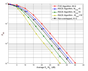
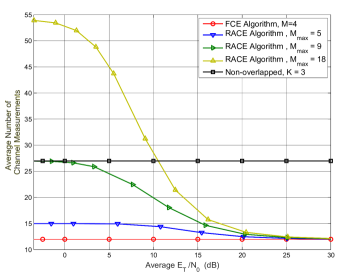
Refer to caption
Refer to caption
Figure 8: Numerical performance results of the proposed algorithms compared to the non-overlapped algorithm presented in [5] for (a) probability of estimation error (PEE) and (b) average number of measurements required for channel estimation.

By using the aforementioned approach and by denoting KTsubscript𝐾𝑇K_{T} and KRsubscript𝐾𝑅K_{R} as the number of sub-ranges at the transmitter and receiver respectively, Fig. 6 shows the average minimum Euclidean distance between the columns of the generator matrix versus M𝑀M for a range of different KTsubscript𝐾𝑇K_{T} and KRsubscript𝐾𝑅K_{R}. Here we constrain the row weights at the transmitter to be WT=KT1subscript𝑊𝑇subscript𝐾𝑇1W_{T}=K_{T}-1 and that at the receiver to be WR=KR1subscript𝑊𝑅subscript𝐾𝑅1W_{R}=K_{R}-1. We can see from this figure that for a fixed KTsubscript𝐾𝑇K_{T} and KRsubscript𝐾𝑅K_{R}, adding additional measurements can increase the spatial separation of the columns in the generator matrix. Based on our analysis, this in turn decreases the probability that one path is mistakenly estimated as another, therefore improving the overall estimation performance. On the other hand, using a larger M𝑀M will require a greater number of channel measurements in each stage. If the FCE algorithm is used, we can increase the value of M𝑀M to improve the estimation performance. If the RACE algorithm is employed, it is generally desired to set M𝑀M relatively low, resulting in a fast estimation that is then confirmed, if needed, by additional measurements. It can also be seen that, when larger values of KTsubscript𝐾𝑇K_{T} and KRsubscript𝐾𝑅K_{R} are employed with a similar M𝑀M, the average minimum Euclidean distances are found to be smaller. This is because these parameters correspond to the estimation of a larger number of sub-range combinations in each stage. Although the energy required for estimation in a single stage may need to be increased for a fixed PEE, the number of over all stages would be less, due to the increased values of K𝐾K.

V-C3 Selection of Mmaxsubscript𝑀𝑚𝑎𝑥M_{max} and ΓΓ\Gamma

Finally, the selection of the maximum number of measurements per stage Mmaxsubscript𝑀𝑚𝑎𝑥M_{max} should be selected based upon any maximum timing constraints. Increasing Mmaxsubscript𝑀𝑚𝑎𝑥M_{max} will significantly increase the energy efficiency at medium to high SNR regime, although the average number of measurements per stage will still converge to M𝑀M at high SNR. We find that, for a fading channel with Gaussian distributed channel coefficients, the selection of ΓΓ\Gamma is not as important as Mmaxsubscript𝑀𝑚𝑎𝑥M_{max}. This is due to the non-zero probability of an outage condition. In general, increasing ΓΓ\Gamma will reduce the PEE by increasing the average number of measurements and therefore expending more energy. In contrast, at high SNR, increasing Mmaxsubscript𝑀𝑚𝑎𝑥M_{max} will allow more measurements to be carried out in the unlikely event that it needs them. Therefore the later uses less average energy.

VI Numerical Results

We now provide some numerical examples to verify the performance of our proposed algorithms. First, we evaluate the impact of the target PEE, ΓΓ\Gamma, on channel estimation performance by comparing the results of the RACE algorithm over a simple single path AWGN channel with K=3𝐾3K=3, M=4𝑀4M=4, and N=3𝑁3N=3 (i.e., single stage). Here we use |α|=PR=1𝛼subscript𝑃𝑅1|\alpha|=P_{R}=1 with varying ΓΓ\Gamma. To show the constant average PEE, here we set Mmax=250subscript𝑀𝑚𝑎𝑥250M_{max}=250 so that even at low SNR, the achieved PEE is unaffected by the number of measurements saturating to its maximum. In addition, as the channel is AWGN, there will also be no chance of a “deep fade” where measurements may continue indefinitely. From Fig. 7 (a) and (b), we can see that the RACE algorithm increases the number of measurements in attempt to hold the PEE below the target value. We also see that the PEE achieved is normally lower than the target PEE. This is largely because the target PEE is actually the highest allowable PEE, for which no additional measurements are required. As such, the average PEE is the average of many channel estimations with performance better than this target. Furthermore, in some cases (particularly in mid-SNR where the number of measurements are low), a single additional measurement on the correct sub-range will significantly increase the PEE beyond the target PEE. We see that this effect diminishes at low SNR where the significance of additional measurements is not as large as that in medium to high SNR. That is, the average PEE is closer to the target PEE.

We now consider a mmWave system with N=27𝑁27N=27 antennas at both the transmitter and receiver. We use a single path channel with fading coefficient, α𝛼\alpha, assumed to follow a complex Gaussian distribution with zero mean and variance PR=1subscript𝑃𝑅1P_{R}=1. We assume the corresponding AOD, ϕlt𝒰Nsuperscriptsubscriptitalic-ϕ𝑙𝑡subscript𝒰𝑁\phi_{l}^{t}\in\mathcal{U}_{N}, and AOA, ϕlt𝒰Nsuperscriptsubscriptitalic-ϕ𝑙𝑡subscript𝒰𝑁\phi_{l}^{t}\in\mathcal{U}_{N}, to follow a random uniform distribution. We set K=3𝐾3K=3 for both of our algorithms and the non-overlapped multi-stage algorithm in [5], all requiring S=3𝑆3S=3 stages. K2=9superscript𝐾29K^{2}=9 measurements are required in each stage of [5]. However, in our proposed algorithms, only M=4𝑀4M=4 time slots are involved in each stage the FCE algorithm and a minimum of M=4𝑀4M=4 for the RACE algorithm. The performance of the RACE algorithm is shown for a number of different values of maximum measurements, Mmaxsubscript𝑀𝑚𝑎𝑥M_{max}, and uses a target PEE of Γ=102Γsuperscript102\Gamma=10^{-2}. Power allocation among S=3𝑆3S=3 stages is applied to all algorithms as (101).

Fig. 8(a) shows the probability of an incorrect AOD/AOA estimate after the S𝑆S stages of estimation have been carried out and Fig. 8(b) shows the average total number of measurements required for the same estimation. The total energy required in the overall channel estimation process is calculated by ET=s=1SPs(M+R)subscript𝐸𝑇superscriptsubscript𝑠1𝑆subscript𝑃𝑠𝑀𝑅E_{T}=\sum_{s=1}^{S}P_{s}(M+R). We can see that, to achieve the same PEE as that in [5], the FCE algorithm requires 2.5dB more energy for a given noise power N0subscript𝑁0N_{0}. However, the number of required channel measurements is decreased by a factor of 2.25.

For the RACE algorithm, we can also see that with Mmax=5subscript𝑀𝑚𝑎𝑥5M_{max}=5, while still significantly faster than [5], it has an improved energy gain for a given PEE compared to Mmax=4subscript𝑀𝑚𝑎𝑥4M_{max}=4, but still worse than than [5] by about 1dB. When Mmaxsubscript𝑀𝑚𝑎𝑥M_{max} is increased to Mmax=K2=9subscript𝑀𝑚𝑎𝑥superscript𝐾29M_{max}=K^{2}=9, we can observe from Fig. 8(a) that the required energy in this case is around 2.5dB better than [5]. From Fig. 8(b) we see that when Mmax=K2=9subscript𝑀𝑚𝑎𝑥superscript𝐾29M_{max}=K^{2}=9 is used, the RACE algorithm is always faster than [5] and, at medium to high SNR (i.e., ET/N0>25subscript𝐸𝑇subscript𝑁025E_{T}/N_{0}>25), the average number of channel measurements converges to SM𝑆𝑀SM. That is, using the proposed RACE algorithm with Mmax=K2subscript𝑀𝑚𝑎𝑥superscript𝐾2M_{max}=K^{2} achieves 2.25 factor reduction of channel measurements while also achieving an energy gain of 2.52.52.5dB for a given probability of error. Further increasing the maximum number of measurements to Mmax=2K2=18subscript𝑀𝑚𝑎𝑥2superscript𝐾218M_{max}=2K^{2}=18 (i.e., the algorithm at most requires twice the measurements required of [5]) we see that the RACE algorithm achieves an energy gain of 6dB compared to [5] at medium to high SNR, while requiring an average of 2.25 times less channel measurements. Furthermore, we can observe from SNR’s greater than 10.5dB that the average number of measurements required in the RACE algorithm is also less than that required by the algorithm in [5].
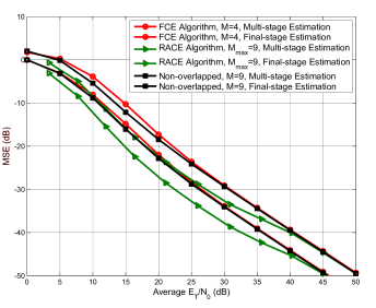
Refer to caption
Figure 9: Numerical performance results of the proposed algorithms compared to the non-overlapped presented in [5] for estimation of the fading coefficient, α𝛼\alpha. Results are shown for estimation using just the final stage of estimation and for the the multi-stage approach shown in III-F. The average estimation error is expressed in dB as E[|αα^|2]Edelimited-[]superscript𝛼^𝛼2\text{E}[{|\alpha-\hat{\alpha}|^{2}]}.

Fig. 9 shows the relative MSE in dB of the fading coefficient α𝛼\alpha, i.e., E[|αα^|2]Edelimited-[]superscript𝛼^𝛼2\text{E}[{|\alpha-\hat{\alpha}|^{2}]}. As can be seen, the LMMSE estimator proposed in section III-F is compared to the one only using measurements from final stage estimation. We can see that the multi-stage LMMSE estimator improves the performance accuracy of the fading coefficient estimation for all algorithms. In the low SNR range, we also see that the proposed FCE algorithm has slightly worse estimation accuracy when compared to [5]. This is predominantly caused by the FCE algorithm having a worse PEE for the same SNR. This performance loss diminishes at mid to high SNR due to the inherent spread of energy over multiple sub-range combinations in the overlapped beam pattern design. For example, in the event that the FCE algorithm selects an incorrect angular range in the final stage, the next most likely sub-range will usually still contain some information of α𝛼\alpha. Focusing on the medium SNR range, Fig. 9 also shows that the RACE algorithm with Mmax=K2=9subscript𝑀𝑚𝑎𝑥superscript𝐾29M_{max}=K^{2}=9 is able to estimate the fading coefficient more accurately when compared to both the FCE algorithm and the algorithm in [5]. This is because, after the additional measurements are directed onto the most likely propagation path. This, in turn, increases the final estimation accuracy once the AOD/AOA have been determined. As the average number of these additional measurements converges to zero at high SNR, this performance gain is lost at high SNR. Interestingly, at high SNR, it can be seen that all approaches converge to a similar path coefficient MSE performance, despite having different PEE. This is largely because when each algorithm identifies an incorrect AOA/AOA, it is usually when the channel is in a deep fade. As a result, misestimating the path coefficient in this case has little effect on overall MSE of the channel fading coefficient. As such, PEE is really a better performance metric for beam misalignment.

We now test the performance of the proposed algorithms under multipath scenarios. Similarly, with [5], we simulate the cases with L=2𝐿2L=2 paths, shown in Fig. 10 (a) and (b), respectively and with L=3𝐿3L=3 paths, shown in Fig. 11 (a) and (b), respectively. In these figures, the most immediate observation is that the FCE algorithm reaches an error floor at high SNR. This is mainly because the non-zero probability of two or more paths having similar magnitude and being in both the non-overlapped sub-ranges. In this scenario, the received measurement vector will be similar to one very strong path in the overlapped region. This is largely the motivation for the RACE algorithm as it permits an additional measurement to confirm the true sub-range combination corresponding to one of the propagation paths. As can be observed in these two figures, the RACE algorithm is able to seamlessly adapt to this scenario, still yielding up to a 5dB gain compared to [5] and converging on being almost 2.25 times faster on average. It is worth noting that this time advantage is only possible with the initial overlapped beam pattern design of the FCE algorithm. That is, the RACE algorithm still needs the initial beam pattern design of FCE to be faster than [5]. Finally, similarly to [5], we can also see that the performance of RACE increases slightly as the number of paths increases from L=1𝐿1L=1 to L=3𝐿3L=3. This is understandable since the chance of detecting one of multiple paths is greater than the chance of detecting a single one.

VII Conclusion

In this paper we have proposed a novel fast channel estimation algorithm for mmWave communication systems based on a novel overlapped beam pattern design. In general, our proposed algorithm can speed up the channel estimation process by a factor of K2/Msuperscript𝐾2𝑀K^{2}/M when compared to existing algorithms with non-overlapped beam patterns. Using a fixed number of measurements, we show that this reduction of measurements comes at an energy-to-noise ratio expense of 2.5dB in order to achieve the same probability of estimation error (PEE). For channels with rapidly changing channel information, this cost may be justified in order to improve the estimation speed. We have also proposed a novel rate-adaptive channel estimation algorithm, in which additional measurements are carried out when a high probability of estimation error is expected. We show that by taking this approach, the channel can be estimated more efficiently, yielding significant gains of up to 6dB when compared to the algorithm in [5], while still converging to the same average number of measurements as the fast channel estimation (FCE) algorithm at high SNR.
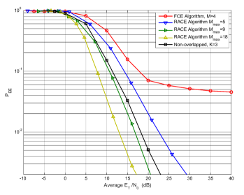
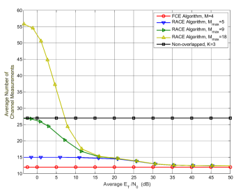
Refer to caption
Refer to caption
Figure 10: The performance comparison between the proposed algorithms with those in [5] in terms of (a) probability of estimation error (PEE) and (b) average number of measurements required for channel estimation for the case L=2𝐿2L=2.
Refer to caption
Refer to caption
Figure 11: The performance comparison between the proposed algorithms with those in [5] in terms of (a) probability of estimation error (PEE) and (b) average number of measurements required for channel estimation for the case L=3𝐿3L=3.

References

  • [1] M. Kokshoorn, P. Wang, Y. Li, and B. Vucetic, “Fast channel estimation for millimetre wave wireless systems using overlapped beam patterns,” in IEEE Int. Conf. on Commun. (ICC), June 2015, pp. 1304–1309.
  • [2] M. Kokshoorn, H. Chen, Y. Li, and B. Vucetic, “RACE: a rate adaptive channel estimation approach for millimeter wave MIMO systems,” in Proc. IEEE Global Telecomm. Conf.   IEEE, Dec. 2016, pp. 1–6.
  • [3] Z. Pi and F. Khan, “An introduction to millimeter-wave mobile broadband systems,” IEEE Commun. Mag., vol. 49, no. 6, pp. 101–107, June 2011.
  • [4] T. S. Rappaport, S. Sun, R. Mayzus, H. Zhao, Y. Azar, K. Wang, G. N. Wong, J. K. Schulz, M. Samimi, and F. Gutierrez, “Millimeter wave mobile communications for 5G cellular: It will work!” IEEE Access, vol. 1, pp. 335–349, May 2013.
  • [5] A. Alkhateeb, O. El Ayach, G. Leus, and R. Heath, “Channel estimation and hybrid precoding for millimeter wave cellular systems,” IEEE J. Sel. Topics Signal Process., vol. 8, no. 5, pp. 831–846, Oct. 2014.
  • [6] W. Hong, K.-H. Baek, Y. Lee, Y. Kim, and S.-T. Ko, “Study and prototyping of practically large-scale mmwave antenna systems for 5g cellular devices,” IEEE Commun. Mag., vol. 52, no. 9, pp. 63–69, 2014.
  • [7] S. Rangan, T. Rappaport, and E. Erkip, “Millimeter-wave cellular wireless networks: Potentials and challenges,” Proc. IEEE, vol. 102, no. 3, pp. 366–385, March 2014.
  • [8] H. Zhang, S. Venkateswaran, and U. Madhow, “Channel modeling and MIMO capacity for outdoor millimeter wave links,” in Proc. Wireless Commun. Netw. Conf. (WCNC), Apr. 2010, pp. 1–6.
  • [9] E. Torkildson, H. Zhang, and U. Madhow, “Channel modeling for millimeter wave mimo,” in Proc. Inf. Theory Appl. Workshop.   IEEE, 2010, pp. 1–8.
  • [10] S. Hur, T. Kim, D. Love, J. Krogmeier, T. Thomas, and A. Ghosh, “Millimeter wave beamforming for wireless backhaul and access in small cell networks,” IEEE Trans. Commun., vol. 61, no. 10, pp. 4391–4403, Oct. 2013.
  • [11] B. Biglarbegian, M. Fakharzadeh, D. Busuioc, M.-R. Nezhad-Ahmadi, and S. Safavi-Naeini, “Optimized microstrip antenna arrays for emerging millimeter-wave wireless applications,” IEEE Trans. Antennas Propag., vol. 59, no. 5, pp. 1742–1747, 2011.
  • [12] “Wireless medium access control (MAC) and physical layer (PHY) specifications for high rate wireless personal area networks (WPANs), amendement 2: Millimeter-wave-based alternative physical layer extension,” IEEE Std 802.15.3c, pp. c1–187, Oct 2009.
  • [13] J. Wang, Z. Lan, C.-W. Pyo, T. Baykas, C.-S. Sum, M. Azizur Rahman, R. Funada, F. Kojima, I. Lakkis, H. Harada, and S. Kato, “Beam codebook based beamforming protocol for multi-gbps millimeter-wave WPAN systems,” in IEEE J. Select. Areas Commun., 2009, pp. 1390–1399.
  • [14] L. Chen, Y. Yang, X. Chen, and W. Wang, “Multi-stage beamforming codebook for 60GHz WPAN,” in Proc. 6th Int. ICST Conf. Commun. Network. China, Aug. 2011, pp. 361–365.
  • [15] A. Sayeed, “Deconstructing multiantenna fading channels,” IEEE Trans. Sig. Process., vol. 50, no. 10, pp. 2563–2579, Oct. 2002.
  • [16] Z. Hong, K. Liu, R. W. Heath Jr, and A. M. Sayeed, “Spatial multiplexing in correlated fading via the virtual channel representation,” IEEE J. Select. Areas Commun.,, vol. 21, no. 5, pp. 856–866, 2003.
  • [17] J. C. Lagarias, J. A. Reeds, M. H. Wright, and P. E. Wright, “Convergence properties of the nelder–mead simplex method in low dimensions,” SIAM J. Optim., vol. 9, no. 1, pp. 112–147, 1998.
  • [18] J. Mo, P. Schniter, N. Gonzalez Prelcic, and R. Heath, “Channel estimation in millimeter wave mimo systems with one-bit quantization,” in Proc. Conf. Signals, Syst. Comput., Nov 2014, pp. 957–961.
  • [19] J. Seo, Y. Sung, G. Lee, and D. Kim, “Pilot beam sequence design for channel estimation in millimeter-wave MIMO systems: A POMDP framework,” in Proc. IEEE Signal Process. Adv. Wireless Commun., June 2015, pp. 236–240.
  • [20] G. MacCartney and T. Rappaport, “73 GHz millimeter wave propagation measurements for outdoor urban mobile and backhaul communications in New York City,” in IEEE Int. Conf. on Commun. (ICC), June 2014, pp. 4862–4867.
  • [21] M. Akdeniz, Y. Liu, M. Samimi, S. Sun, S. Rangan, T. Rappaport, and E. Erkip, “Millimeter wave channel modeling and cellular capacity evaluation,” IEEE J. Select. Areas Commun., vol. 32, no. 6, pp. 1164–1179, June 2014.
  • [22] W. Bajwa, J. Haupt, A. Sayeed, and R. Nowak, “Compressed channel sensing: A new approach to estimating sparse multipath channels,” Proc. IEEE, vol. 98, no. 6, pp. 1058–1076, June 2010.
  • [23] “Wireless medium access control (mac) and physical layer (phy) specifications for high rate wireless personal area networks (WPAN)s, amendement 2: Millimeter-wave-based alternative physical layer extension, IEEE standard 802.15.3c,” Oct. 2009.
  • [24] Y. Tsang, A. Poon, and S. Addepalli, “Coding the beams: Improving beamforming training in mmwave communication system,” in Proc. IEEE Global Telecomm. Conf., Dec 2011, pp. 1–6.
  • [25] X. Zhang, A. Molisch, and S.-Y. Kung, “Variable-phase-shift-based RF-baseband codesign for mimo antenna selection,” IEEE Trans. Signal Process., vol. 53, no. 11, pp. 4091–4103, Nov 2005.
  • [26] Z. Xiao, T. He, P. Xia, and X.-G. Xia, “Hierarchical codebook design for beamforming training in millimeter-wave communication,” IEEE Trans. Commun., vol. 15, no. 5, pp. 3380–3392, 2016.
  • [27] P. Xia, S.-K. Yong, J. Oh, and C. Ngo, “Multi-stage iterative antenna training for millimeter wave communications,” in Proc. IEEE Global Telecomm. Conf.   IEEE, 2008, pp. 1–6.
  • [28] Z. Xiao, X.-G. Xia, D. Jin, and N. Ge, “Iterative eigenvalue decomposition and multipath-grouping tx/rx joint beamformings for millimeter-wave communications,” IEEE Trans. Commun., vol. 14, no. 3, pp. 1595–1607, 2015.
  • [29] Z. Xiao, L. Bai, and J. Choi, “Iterative joint beamforming training with constant-amplitude phased arrays in millimeter-wave communications,” IEEE Commun. Letters, vol. 18, no. 5, pp. 829–832, 2014.
  • [30] P. Xia, H. Niu, J. Oh, and C. Ngo, “Practical antenna training for millimeter wave mimo communication,” in IEEE Vehicular Technology Conference, 2008.
  • [31] A. Sayeed and V. Raghavan, “The ideal MIMO channel: Maximizing capacity in sparse multipath with reconfigurable arrays,” in Proc. ISIT, July 2006, pp. 1036–1040.
  • [32] J. G. Proakis, Digital communications.   New York, NY, USA: McGraw-Hill, 1995.
  • [33] R. G. Gallager, “Circularly-symmetric gaussian random vectors,” preprint, pp. 1–9, 2008.
  • [34] R. D. Bock and M. Aitkin, “Marginal maximum likelihood estimation of item parameters: Application of an em algorithm,” Psychometrika, vol. 46, no. 4, pp. 443–459, 1981.
  • [35] L. L. Scharf, Statistical signal processing.   Addison-Wesley Reading, MA, 1991, vol. 98.
  • [36] G. L. Stüber, Principles of mobile communication.   Springer Science & Business Media, 2011.
  • [37] C. E. Shannon, “A mathematical theory of communication,” Bell Syst. Tech. J., vol. 27, p. 379–423, 1948.
  • [38] T. Bai, A. Alkhateeb, and R. Heath, “Coverage and capacity of millimeter-wave cellular networks,” IEEE Commun. Mag., vol. 52, no. 9, pp. 70–77, 2014.