Optimal Geographic Caching in Finite Wireless Networks

Abstract

Cache-enabled device-to-device (D2D) networks turn memory of the devices at the network edge, such as smart phones and tablets, into bandwidth by enabling asynchronous content sharing directly between proximate devices. Limited storage capacity of the mobile devices necessitates the determination of optimal set of contents to be cached on each device. In order to study the problem of optimal cache placement, we model the locations of devices in a finite region (e.g., coffee shop, sports bar, library) as a uniform binomial point process (BPP). For this setup, we first develop a generic framework to analyze the coverage probability of the target receiver (target-Rx) when the requested content is available at the $k^{th}$ closest device to it. Using this coverage probability result, we evaluate optimal caching probability of the popular content to maximize the total hit probability. Our analysis concretely demonstrates that optimal caching probability strongly depends on the number of simultaneously active devices in the network.

I Introduction

Video-driven applications, such as on-demand video streaming and mobile television, are primary drivers of the explosion in mobile data traffic [1]. Empirical studies of the distribution of video requests reveals a high degree of spatiotemporal correlation in the content demanded, which means that a few popular videos are requested by multiple users at different times [2]. However, the current cellular network do not exploit this spatiotemporal correlation exhibited in the content demand, which can be effectively used as an active part of the future networks design. In particular, popular contents can be locally cached at the edge of the network such as in small cell base stations (BSs) or mobile devices and then delivered over a direct link to the user who requests them [3, 4, 5]. However, limited storage capacity of the edge devices necessitates the need for developing optimal caching strategies. While this problem has been addressed for infinite networks in [6, 7, 8, 9, 10], more relevant D2D use case of finite networks has not yet been addressed in the literature. The modeling and performance analysis of optimal geographical caching in finite wireless networks is therefore the main focus of this paper.

Related work. Modeling and analysis of the cache-enabled heterogeneous networks (HetNets) including small cell BSs and mobile devices have taken two main directions in the literature. The first line of work focuses on the fundamental throughput scaling results by assuming simple protocol channel model, where communication between two nodes is successful if they are within the fixed collaboration distance [11, 12]. The second line of work which is also relevant to the current work considers a more realistic model for the underlying physical layer, where the successful communication depends on physical quantities such as the path-loss, fading, and interference power. More specifically, these works focus on optimal cache-placement strategies in D2D or ultra-dense HetNets by using the tools from stochastic geometry [6, 7, 8, 9, 10]. The most popular technical approach amongst these works is modeling the locations of nodes (devices or small cell BSs) as an infinite homogenous Poisson Point Process (PPP) and assume that each device connects to its closest possible serving node. The main reason behind the popularity of this approach is the simplicity involved in the mathematical analysis as demonstrated in [13]. This setup albeit relevant for the traditional cellular architecture, is not adequate in D2D and ultra-dense cache-enabled HetNets where the content of interest may not necessarily be available at the closest node (device or small cell BS) to the target-Rx. Relaxing this constraint, [6] defined an optimization problem that determines the optimal caching strategy using the $k$-coverage results for an infinite PPP derived in [14]. In continuation to [6], we determine the optimal geographic caching strategy for finite wireless networks in this paper. To the best of our understanding, this is the first work on optimal caching in finite networks. More details are provided next.

Contributions and outcomes. We model the locations of devices in a finite wireless network as a uniform-BPP. For this setup, we develop a new set of tools to characterize the “exact” expression of the coverage probability where the serving device is the $k^{th}$ closest device to the target-Rx out of the $N^{\tt t}$ transmitting devices. To perform this analysis, we prove that the distance from interfering devices conditioned on the location of the serving device are independently and identically distributed (i.i.d.). Using this i.i.d. property, we derive a closed-form expression for the Laplace transform of interference distribution that is the main component of the coverage probability analysis. This coverage probability result for finite networks is analogous to the $k$-coverage result of [14] and can be easily incorporated into the optimization formulation of [6] in order to characterize throughput and determine the optimal caching strategy that maximizes total hit probability in finite networks. Our analysis demonstrates that the increasing number of active devices has a conflicting effect on the maximum hit probability and the throughput: maximum hit probability decreases and throughput increases. This shows that more and more devices can be simultaneously activated as long as the hit probability remains acceptable.

II System Model

System setup and key assumption

We consider a cache-enabled D2D network comprising $N^{\tt t}+1$ devices that include target-Rx and $N^{\tt t}$ transmitting devices. Modeling the locations of transmitting devices as a uniform-BPP $\{{\bf y}_{i}\}\equiv\Phi_{\tt t}$, we assume that $N^{\tt t}$ transmitting devices are independently and uniformly distributed in the ball of radius $r_{\rm d}$ centered at origin, which is denoted by ${\bf b}(0,r_{\rm d})$. We further assume that $N^{\rm a}$ out of $N^{\tt t}$ transmitting (serving and interfering) devices simultaneously reuse the same resource block. The locations of simultaneously active devices is denoted by $\Phi_{\rm a}$. For this setup, we perform analysis on a target-Rx located at origin. Note that while our analysis is, in principle, extensible to any arbitrarily located target-Rx, we limit it to this case due space constrains. The analysis corresponding to the arbitrarily located target-Rx will be provided in the extended version of this paper.

Channel model

In order to pose an optimization problem similar to [6] for finite networks, we are interested in the case where the content of interest for the target-Rx is available at its $k^{th}$ closest device out of $N^{\tt t}$ transmitting devices, where $1\leq k\leq N^{\tt t}$. Fixing the location of this serving device which is denoted by ${\bf y}_{k}$, we assume that the interfering devices, located at ${\bf y}_{i}\in\Phi_{\rm a}\setminus{\bf y}_{k}\subset\Phi_{\tt t}$, are chosen uniformly at random from the set of transmitting devices. To keep the notation simple, we assume that the thermal noise is negligible compared to the interference and is hence ignored. So, the signal to interference ratio ($\mathtt{SIR}$) is:

$$\mathtt{SIR}=\frac{h_{k}\|{\bf y}_{k}\|^{-\alpha}}{\sum_{{\bf y}_{i}\in\Phi_{\rm a}\setminus{\bf y}_{k}}h_{i}\|{\mathbf{y}}_{i}\|^{-\alpha}},$$ (1)

where $h_{i}\sim\exp(1)$ and $\|.\|^{-\alpha}$ model Rayleigh fading and power law path-loss with exponent $\alpha>2$, respectively.

Remark 1 (Scale invariance of BPP network).

The $\mathtt{SIR}$ as defined in (1) is independent of the network radius $r_{\rm d}$ because both serving and interfering devices are chosen from the same point process. This is mainly because by changing $r_{\rm d}$, all distances scale with the same parameter. So, without loss of generality, we normalize $r_{\rm d}$ to $1$.

Content popularity

We consider a finite library of popular contents ${\cal C}=\{{c}_{1},c_{2},...,c_{\cal J}\}$ with size ${\cal J}$, where $c_{j}$ denotes the $j^{th}$ most popular content. For simplicity of exposition, we assume that all the content has the same size, which is normalized to one. We further assume that the transmitting devices are equipped with cache storage of size $m_{\rm c}$ and hence each device can store at most $m_{\rm c}$ popular contents. Now, denoting the specific set of contents at a generic transmitting device by $\Omega$, the caching probability is: $b_{j}=\mathbb{P}(c_{j}\in\Omega),$ where $b_{j}$ denotes the probability that the content $c_{j}$ is stored at a given transmitting device. To model the content popularity in this system, we use Zipf’s distribution due to its practical relevance [2]. Hence, the request probability for file $c_{j}$ is:

$${\tt P}_{R_{j}}=\frac{j^{-\gamma}}{\sum_{i=1}^{\cal J}i^{-\gamma}};\quad 1\leq j\leq{\cal J},$$ (2)

where $\gamma$ represents the parameter of Zipf’s distribution.

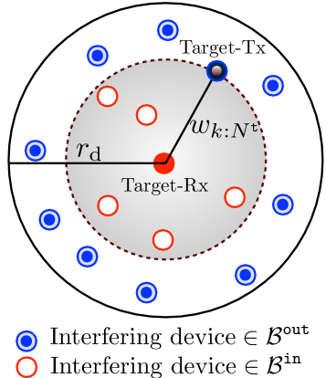
Figure 1: Illustration of the system model.

III Optimal content placement

This is the main technical section of this paper, where we characterize network performance in terms of total hit probability, coverage probability, and network throughput. Before going into the detailed analyses of these metrics, we first characterize the distribution of the distances from the target-Rx to the transmitting devices in the next subsection.

III-A Relevant Distance Distributions in a BPP

In our setup, the target-Rx is assumed to be located at the origin while the transmitting devices are uniformly and independently distributed in ${\bf b}(0,r_{d})$. Therefore, it is easy to infer that the sequence of distances from transmitting devices to the target-Rx which is denoted by $\{W_{i}=\|{\bf y}_{i}\|\}$ contains i.i.d. elements with PDF and CDF given by [15]:

$$\text{PDF}:\quad f_{W_{i}}(w_{i})=\frac{2w_{i}}{r_{\rm d}^{2}};\quad 0\leq w_{i}\leq r_{\rm d},$$ (3)

$$\text{CDF}:\quad F_{W_{i}}(w_{i})=\frac{w_{i}^{2}}{r_{\rm d}^{2}};\quad 0\leq w_{i}\leq r_{\rm d}.$$ (4)

Recall that the serving device is the $k^{th}$ closest transmitting device to the target-Rx. In order to characterize the serving distance distribution, we need to “order” the distances from transmitting devices to the target-Rx. We define an ordered set $\{w_{i:N^{\tt t}}\}_{i=1:N^{\tt t}}$ by sorting $w_{i}$-s in ascending order such that $w_{1:N^{\tt t}}<w_{2:N^{\tt t}}<...<w_{N^{\tt t}:N^{\tt t}}.$ Now, using the i.i.d. property of the sequence $\{W_{i}\}$, the PDF of the serving distance $R=W_{k:N^{\tt t}}$ is:

$$f_{R}^{(k)}(r)=\frac{N^{\rm t}!}{(k-1)!(N^{\rm t}-k)!}{F_{W_{i}}(r)}^{k-1}\\ \times f_{W_{i}}(r)(1-F_{W_{i}}(r))^{N^{\rm t}-k},$$ (5)

where, $f^{(k)}_{R}(r)$ can be obtained simply from the PDF of the $k$ order statistics of the sequence $\{W_{i}\}$ [16]. It is worth highlighting that the interfering devices can lie at any place except the location of the serving device. This means that the $k^{th}$ closest transmitting device to the target receiver is explicitly removed from the interference field. In order to incorporate this in the analysis, we partition the set of distances from transmitting devices to the target-Rx into three subsets ${\cal B}=\{{\mathcal{B}}^{\tt in},w_{k:N^{\tt t}},{\mathcal{B}}^{\tt out}\}$ such that ${\mathcal{B}}^{\tt in}$ and ${\mathcal{B}}^{\tt out}$ represent the set of potential interfering devices closer and farther to the target-Rx respectively, compared to the serving device. This setup is illustrated in Fig. 1. The following Lemma deals with conditional i.i.d. property of $U_{\tt in}\in{\mathcal{B}}^{\tt in}$ and $U_{\tt out}\in{\mathcal{B}}^{\tt out}$, and provides their density functions. The proof is provided in Appendix -A.

Lemma 1.

The sequences of random variables $U_{\tt in}\in{\mathcal{B}}^{\tt in}$ and $U_{\tt out}\in{\mathcal{B}}^{\tt out}$ conditioned on $r=w_{k:N^{\tt t}}$ are independent. Moreover,

i) the elements in sequence $U_{\tt in}\in{\mathcal{B}}^{\tt in}$ conditioned on $r=w_{k:N^{\tt t}}$ are i.i.d., where the PDF of each element is:

$$f_{U_{\tt in}}(u_{\tt in}|r)=\left\{\begin{array}[]{cc}\frac{f_{W_{i}}(u_{\tt in})}{F_{W_{i}}(r)},&u_{\rm in}<r\\ 0,&u_{\tt in}\geq r\end{array}\right.,$$ (8)

ii) the elements in sequence $U_{\tt out}\in{\mathcal{B}}^{\tt out}$ conditioned on $r=w_{k:N^{\tt t}}$ are i.i.d., where the PDF of each element is:

$$f_{U_{\rm out}}(u_{\tt out}|r)=\left\{\begin{array}[]{cc}\frac{f_{W_{i}}(u_{\tt out})}{1-F_{W_{i}}(r)},&u_{\tt out}>r\\ 0,&u_{\rm out}\leq r\end{array}\right.,$$ (11)

where $f_{W_{i}}(.)$ and $F_{W_{i}}(.)$ are given by (3) and (4), respectively.

In [17, 18], we proved a similar i.i.d. property for the distribution of distances in Thomas cluster process. The conditional i.i.d. property of $U_{\tt in}\in{\mathcal{B}}^{\tt in}$ and $U_{\tt out}\in{\mathcal{B}}^{\tt out}$ is the key enabler for the analysis of the Laplace transform of interference, which is discussed in the next subsection.

III-B Laplace Transform of Interference Distribution

As will be evident in the sequel, the characterization of Laplace transform of interference distribution is the key intermediate step in the coverage probability analysis. The “exact” closed-form expression of the Laplace transform of interference where serving device is the $k^{th}$ closest transmitting device to the target-Rx is given in the next Lemma. The proof is provided in Appendix -B.

Lemma 2.

The Laplace transform of interference distribution conditioned on the serving distance $r=w_{k:N^{\tt t}}$ is ${\mathcal{L}}_{{\mathcal{I}}}^{(k)}(s|r)=$

$$\sum_{\ell=0}^{n^{\rm a}_{m}}\xi(p,n^{\rm a}_{m})\left(\frac{{\cal C}(\alpha,s,r)}{r^{2}}\right)^{\ell}\left(\frac{{\cal C}(\alpha,s,r_{\rm d})-{\cal C}(\alpha,s,r)}{r_{\rm d}^{2}-r^{2}}\right)^{N^{\rm a}-\ell-1}$$

$$\text{with}\quad{{\cal C}(\alpha,s,x)}=x^{2}-x^{2}\>{}_{2}F_{1}(1,\frac{2}{\alpha},1+\frac{2}{\alpha},{-x^{\alpha}/s})),$$ (12)

where $\xi(p,n^{\rm a}_{m})=\frac{p^{\ell}(1-p)^{N^{\rm a}-\ell-1}\binom{N^{\rm a}-1}{\ell}}{\sum_{\ell=0}^{N^{\rm a}_{m}}p^{\ell}(1-p)^{N^{\rm a}-\ell-1}\binom{N^{\rm a}-1}{\ell}}$, $p=\frac{k-1}{N^{\tt t}-1}$, $n^{\rm a}_{m}=\min(k-1,N^{\rm a}-1)$, and ${}_{2}F_{1}(a,b;c;z)=1+\sum_{k=1}^{\infty}\frac{z^{k}}{k!}\prod_{l=0}^{k-1}\frac{(a+l)(b+l)}{c+l}$.

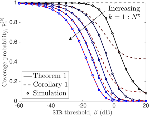
Figure 2: Coverage probability as a function of $\mathtt{SIR}$ threshold ($\alpha=4$, and $N^{\rm a}=N^{\tt t}=5$).

III-C Coverage Probability

Coverage probability is defined as the probability that $\mathtt{SIR}$ exceeds predefined threshold needed to establish a successful connection. The coverage probability of the target-Rx in a finite network is derived in the next Theorem.

Theorem 1.

Using the expression of Laplace transform of interference distribution given by (12), the coverage probability of the target-Rx is:

$${\tt P}_{c}^{(k)}=\int_{0}^{r_{\rm d}}{\mathcal{L}}_{{\mathcal{I}}}^{(k)}(\beta r^{\alpha}|r)f_{R}^{(k)}(r){\rm d}r,$$ (13)

where $f_{R}^{(k)}(r)$ given by (5), and $\beta$ is target $\mathtt{SIR}$ threshold.

Proof:

Using the definition of coverage probability, i.e., $\mathbb{P}(\mathtt{SIR}\geq\beta)=\mathbb{P}\big{(}h_{k}\geq\beta r^{\alpha}{\sum_{{\bf y}_{i}\in\Phi_{\rm a}\setminus{{\bf y}_{k}}}h_{i}\|{\mathbf{y}}_{i}\|^{-\alpha}}\big{)}$

$$\stackrel{{\scriptstyle(a)}}{{=}} \mathbb{E}_{R}\Big{[}\exp\Big{(}-\beta r^{\alpha}{\sum_{{\bf y}_{i}\in\Phi_{\rm a}\setminus{\bf y}_{k}}h_{i}\|{\mathbf{y}}_{i}\|^{-\alpha}}\Big{)}\big{|}R\Big{]}$$

where $(a)$ follows from $h_{0}\sim\exp(1)$. The final result follows from the definition of Laplace transform, followed by de-conditioning over serving distance $R$. ∎

Using the result of Theorem 1, we now derive a closed-form upper bound on the coverage probability in the next Corollary. The result can be readily derived by ignoring the contribution of interference from interfering devices farther than the serving device to the target-Rx, and substituting $s=\beta r^{\alpha}$ in the expression of Laplace transform interference distribution given by (12).

Corollary 1.

The coverage probability of a target-Rx is upper bounded by

$${\tt P}_{c}^{(k)}\leq\sum_{\ell=0}^{n^{\rm a}_{m}}\xi(p,n^{\rm a}_{m})\left((1-{}_{2}F_{1}(1,\frac{2}{\alpha},1+\frac{2}{\alpha},{-\frac{1}{\beta}}))\right)^{\ell}$$ (14)

which for $$N^{\rm a}=N^{\tt t} \alpha=4$$ and simplifies to

$${{\tt P}_{\rm c}}\leq\left(1-\sqrt{\beta}\arctan\left(1/\sqrt{\beta}\right)\right)^{k-1}.$$ (15)

Remark 2.

From Corollary 1, it is clear that the coverage probability has a power-law behavior with the exponent of $k-1$ when all transmitting nodes are simultaneously active.

We plot the coverage probability for different values of $k$ in Fig. 2. It can be seen that the “exact” expression of the coverage probability given by Theorem 1 and the simulation result match perfectly which confirms the accuracy of the analysis. As expected, the closed-form expression given by Corollary 1 gets tight with increasing $k$ while being exact for $k=N^{\tt t}$. The upper bound, however, gets loose with increasing target $\mathtt{SIR}$ threshold. This is mainly because the impact of interfering devices in ${\cal B}^{\tt out}$ on the coverage probability is more prominent for large $\mathtt{SIR}$ threshold.

III-D Total Hit Probability and Throughput

As defined in [6], the total hit probability is the probability that the target-Rx finds its requested content in one of the devices that cover it, which in turn depends on: i) request probability, which is assumed to be known a priori, ii) caching probability, which is dictated by the availability of the popular contents, and iii) coverage probability that guarantees the minimum $\mathtt{SIR}$ for successful reception. Recalling that the caching probability and the request probability for content $c_{j}$ were denoted by $b_{j}$ and ${\tt P}_{R_{j}}$, the total hit probability can be mathematically expressed as:

$${\tt P}_{\rm hit}=\sum_{j=1}^{{\cal J}}{\tt P}_{R_{j}}\sum_{k=1}^{N_{\rm t}}{\tt P}^{(k)}_{{\rm c}}(1-b_{j})^{k-1}b_{j}$$ (16)

where $(1-b_{j})^{k-1}b_{j}$ indicates that the closest device with content of interest is $k^{th}$ closest device to the target-Rx. In other words, the content of interest was not found at $(k-1)$ closet transmitting devices to the target-Rx. On the same lines as [6], the problem of optimal geographic caching in finite wireless networks can be formulated as:

$${\tt P}_{\rm hit}^{*}=\max_{\{b_{j}\}}\sum_{j=1}^{{\cal J}}{\tt P}_{R_{j}}\sum_{k=1}^{N_{\rm t}}{\tt P}^{(k)}_{{\rm c}}(1-b_{j})^{k-1}b_{j}$$ (17)

$$\text{s.t.}\quad\sum_{j=1}^{\cal J}b_{j}\leq m_{\rm c};\quad 0\leq b_{j}\leq 1\>\>\forall j$$ (18)

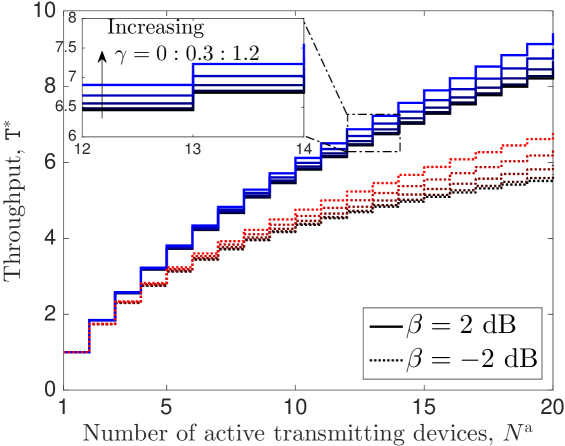
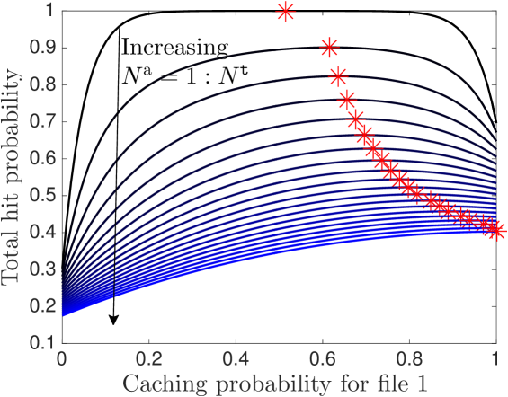
where $P_{c}^{(k)}$ is the new coverage probability result derived in Theorem 1. The necessity and sufficiency of the constraints given by (18) has already been discussed in [6]. For better understanding of this optimization problem, Fig. 3 plots the total hit probability for the simple setup of ${\cal J}=2$, and $m_{\rm c}=1$. It can be seen that by increasing the number of simultaneously active transmitting devices, $N_{\rm a}$, the optimal caching probability for the most popular content (i.e., $b_{1}$) moves toward one. This is mainly because increasing $N_{\rm a}$ results in higher interference, which in turn decreases coverage probability. For example when there is only one active device ( completely orthogonal channel allocation), coverage probability is equal to one under interference limited regime. Hence, it is optimal to cache the two contents with the same probability, i.e., $b_{1}=b_{2}=0.5$. However, by increasing the number of active transmitting devices, ${\tt P}_{\rm c}^{(k)}$ for $k>1$ decreases significantly due to increased interference. As demonstrated in Fig. 3, this makes it optimal to cache the more popular contents more often. Though channel orthogonalization is beneficial in terms of total hit probability, it is not desirable for the network throughput which favors having multiple active links as long as the resulting interference remains acceptable. To study the tradeoff between the number of active links and the resulting interference, we formally define throughput as: ${\tt T}^{*}=N^{\rm a}\>{\tt P}_{\rm hit}^{*}.$
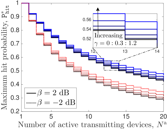
Figs. 4 and 5 plot maximum hit probability and throughput versus number of active transmitting devices, respectively. Interestingly, increasing the number of active devices has a conflicting effect on the maximum hit probability and the throughput: maximum hit probability decreases and throughput increases. This implies that more devices can be simultaneously activated if the total hit probability remains within acceptable limits.

Figure 3: Total hit probability as a function of caching probability for file 1, where asterisk shows optimal hit probability (${\cal J}=2$, $m_{\rm c}=1$, $\alpha=4$, $\beta=0$ dB, $\gamma=1.2$, and $N^{\tt t}=20$)

Figure 4: Maximum hit probability as a function of number of active devices (${\cal J}=2$, $m_{\rm c}=1$, $\alpha=4$, and $N^{\tt t}=20$)

Figure 5: Throughput as a function of number of active devices (${\cal J}=2$, $m_{\rm c}=1$, $\alpha=4$, and $N^{\tt t}=20$)

IV Conclusion

Modeling the locations of the devices as a uniform-BPP, we derive a new coverage result to enable the analysis of optimal geographic caching in finite wireless networks. To the best of our knowledge, this is the first stochastic geometry-based analysis of cache-enabled finite D2D networks. This work has many extensions. From modeling perspective, it can be extended to an arbitrary shape (instead of a circle) where the node locations follow a more general distribution. Further, this framework can be extended to analyze Matérn cluster process where each finite network form one cluster. From system perspective, it can be used for the performance analysis of indoor communication and hotspots, where the analyses based on the infinite PPP assumption may not be applicable.

-A Proof of Lemma 1

The joint density function of “ordered” subset $\{W_{i:N^{\tt t}}\}_{i=1:N^{\tt t}}$ conditioned on $r=w_{k:N^{\tt t}}$ is:

$$f({{w_{1:N^{\tt t}}},...,{w_{N^{\tt t}:N^{\tt t}}}|w_{k:N^{\tt t}}})=\frac{f({{w_{1:N^{\tt t}}},...,{w_{N^{\tt t}:N^{\tt t}}}})}{f_{W_{k:N^{\tt t}}}(w_{k:N^{\tt t}})},$$

$$\stackrel{{\scriptstyle(a)}}{{=}}\frac{N^{t}!\prod_{i=1}^{N^{t}}f_{W_{i}}(w_{i:N^{\tt t}})}{f_{W_{k:N^{\tt t}}}(w_{k:N^{\tt t}})}\stackrel{{\scriptstyle(b)}}{{=}}\underbrace{(k-1)!\prod_{i=1}^{k-1}\frac{f_{W_{i}}(w_{i:N^{\tt t}})}{F_{W}(w_{k:N})}}_{\text{joint PDF of }\{W_{i:N^{\tt t}}\}_{i=1:k-1}}$$

$$\times\underbrace{({N^{t}-k})!\prod_{i=k+1}^{N_{\tt t}}\frac{f_{W_{i}}(w_{i:N^{\tt t}})}{1-F_{W}(w_{k:N})}}_{\text{joint PDF of }\{W_{i:N^{\tt t}}\}_{i=k+1:N^{\tt t}}}$$

where $f_{W_{k:N^{\tt t}}}(.)=f^{(k)}_{R}(.)$. Here $(a)$ follows from definition of the joint PDF of order of statistics [16] with sampling PDF $f_{W_{i}}(.)$ given by (4), and (b) follows from substituting the expression of $f_{W_{k:N^{\tt t}}}(.)$ which is given by (4). The product of joint PDFs in $(b)$ implies that the $\{W_{i:N^{\tt t}}\}_{i=1:k}$ and $\{W_{i:N^{\tt t}}\}_{i=k+1:N^{\tt t}}$ conditioned on the serving distance $r=w_{k:N}$ are independent. Now, the joint PDF of $\{W_{i:N^{\tt t}}\}_{i=1:k}$ conditioned on $r=w_{k:N^{\tt t}}$ is:

$$f({{w_{1:N^{\tt t}}},...,{w_{k-1:N^{\tt t}}}|w_{k:N^{\tt t}}})=(k-1)!\prod_{i=1}^{k-1}\frac{f_{W_{i}}(w_{i:N^{\tt t}})}{F_{W_{i}}(w_{k:N^{\tt t}})}.$$

Note that $(k-1)!$ shows possible permutations of distances from “ordered” subset, $\{w_{i:N^{\tt t}}\}_{i=1:k-1}$, and doesn’t appear in the joint PDF of distances from “unordered” subset ${\mathcal{B}}^{\tt in}$, i.e.,

$$f({{w_{1}},...,{w_{k-1}}|w_{k:N^{\tt t}}})=\prod_{i=1}^{k-1}\frac{f_{W_{i}}(w_{i})}{F_{W_{i}}(w_{k:N^{\tt t}})},\>\>w_{i}\leq w_{k:N^{\tt t}}$$

where the product of same functional form of the joint PDF $f({{w_{1}},...,{w_{k-1}}|w_{k:N^{\tt t}}})$ infers that the subset of distances in “unordered” set ${\mathcal{B}}_{\tt in}$ are i.i.d., with PDF $\frac{f_{W_{i}}(w_{i})}{F_{W_{i}}(w_{k:N^{\tt t}})}$. Denoting the distances in “unordered” subset ${\mathcal{B}}^{\tt in}$ by $u_{\tt in}$, and substituting $w_{k:N^{\tt t}}$ with $r$ completes the proof. Similar arguments can be applied for the derivation of $f_{U_{\rm out}}(.|r)$.

-B Proof of Lemma 2

The Laplace transform of interference conditioned on $r=w_{k:N^{t}}$ is ${\mathcal{L}}_{{\mathcal{I}}}^{(k)}(s|r)$

$$=\mathbb{E}\Big{[}\prod_{u_{\tt in}\in{\mathcal{B}}^{\tt in}}\exp\Big{(}-sh_{i}{u_{\tt in}}^{-\alpha}\Big{)}\prod_{u_{\tt out}\in{\mathcal{B}}^{\tt out}}\exp\Big{(}sh_{i}{u_{\tt out}}^{-\alpha}\Big{)}\Big{]}$$

$$\stackrel{{\scriptstyle(a)}}{{=}}\mathbb{E}\Big{[}\prod_{u_{\tt in}\in{\mathcal{B}}^{\tt in}}\frac{1}{1+s{u_{\tt in}}^{-\alpha}}\prod_{u_{\tt out}\in{\mathcal{B}}^{\tt out}}\frac{1}{1+s{u_{\tt out}}^{-\alpha}}\Big{]}$$

$$\stackrel{{\scriptstyle(b)}}{{=}}\sum_{\ell=0}^{n^{\rm a}_{m}}\frac{p^{\ell}(1-p)^{N^{\rm a}-\ell-1}\binom{N^{\rm a}-1}{\ell}}{\sum_{\ell=0}^{N^{\rm a}_{m}}p^{\ell}(1-p)^{N^{\rm a}-\ell-1}\binom{N^{\rm a}-1}{\ell}}\Bigg{(}\int_{0}^{r}\frac{1}{1+s{u_{\tt in}^{-\alpha}}}\times$$

$$f_{U_{\tt in}}(u_{\tt in}|r){\rm d}u_{\tt in}\Bigg{)}^{\ell}\Bigg{(}\int_{r}^{r_{\rm d}}\frac{1}{1+s{u_{\tt out}^{-\alpha}}}f_{U_{\tt out}}(u_{\tt out}|r){\rm d}u_{\tt out}\Bigg{)}^{N^{\rm a}-\ell-1}$$

where $(a)$ follows from $h_{i}\sim\exp(1)$, and $(b)$ follows from the fact that $U_{\tt in}\in{\mathcal{B}}^{\tt in}$ and $U_{\tt out}\in{\mathcal{B}}^{\tt out}$ are conditionally i.i.d., with PDF $f_{U_{\tt in}}(.|r)$, and $f_{U_{\rm out}}(.|r)$, followed by expectation over the number of devices located in ${\cal B}_{\tt in}$ and ${\cal B}_{\tt out}$, followed by the fact that the number of device in ${\cal B}_{\tt in}$ is binary random variable with probability $p=\frac{k-1}{N^{\tt t}-1}$ conditioned on total being less than $n^{\rm a}_{m}=\min(k-1,N^{\rm a}-1)$. The integral can be solved based on [19, eq (3.194.1)].

References

• [1] Cisco, โ€œGlobal mobile data traffic forecast update, 2013โ€“2018,โ€ white paper, 2014.
• [2] M.ย Cha, H.ย Kwak, P.ย Rodriguez, Y.-Y. Ahn, and S.ย Moon, โ€œI Tube, You Tube, Everybody Tubes: analyzing the worldโ€™s largest user generated content video system,โ€ in Proc., ACM Intl. Conf. on Special Interest Group on Data Commun. (SIGCOMM), 2007.
• [3] N.ย Golrezaei, A.ย F. Molisch, A.ย G. Dimakis, and G.ย Caire, โ€œFemtocaching and device-to-device collaboration: A new architecture for wireless video distribution,โ€ IEEE Commun. Magazine, vol.ย 51, no.ย 4, pp. 142โ€“149, 2013.
• [4] E.ย BaลŸtug, M.ย Bennis, and M.ย Debbah, โ€œLiving on the edge: The role of proactive caching in 5g wireless networks,โ€ IEEE Commun. Magazine, vol.ย 52, no.ย 8, pp. 82โ€“89, 2014.
• [5] S.ย Krishnan, M.ย Afshang, and H.ย S. Dhillon, โ€œMobility-aware caching in ultra- dense heterogeneous cellular networks.โ€ submitted to IEEE Wireless Magazine., 2016.
• [6] B.ย Bล‚aszczyszyn and A.ย Giovanidis, โ€œOptimal geographic caching in cellular networks,โ€ in Proc., IEEE Intl. Conf. on Commun. (ICC), 2015.
• [7] S.ย Krishnan and H.ย S. Dhillon, โ€œDistributed caching in device-to-device networks: A stochastic geometry perspective,โ€ in Proc. Asilomar, Pacific Grove, CA. 2015.
• [8] C.ย Yang, Y.ย Yao, Z.ย Chen, and B.ย Xia, โ€œAnalysis on cache-enabled wireless heterogeneous networks,โ€ IEEE Trans. on Wireless Commun., vol.ย 15, no.ย 1, pp. 131โ€“145, 2016.
• [9] E.ย BaลŸtug, M.ย Bennis, M.ย Kountouris, and M.ย Debbah, โ€œCache-enabled small cell networks: Modeling and tradeoffs,โ€ EURASIP Journal on Wireless Commun. and Networking, no.ย 1, pp. 1โ€“11, 2015.
• [10] D.ย Malak and M.ย Al-Shalash, โ€œOptimal caching for device-to-device content distribution in 5g networks,โ€ in Proc., IEEE Globecom Workshops, 2014, pp. 863โ€“868.
• [11] K.ย Shanmugam, N.ย Golrezaei, A.ย G. Dimakis, A.ย F. Molisch, and G.ย Caire, โ€œFemtocaching: Wireless content delivery through distributed caching helpers,โ€ IEEE Trans. on Info. Theory, vol.ย 59, no.ย 12, pp. 8402โ€“8413, 2013.
• [12] N.ย Golrezaei, P.ย Mansourifard, A.ย Molisch, and A.ย Dimakis, โ€œBase-station assisted device-to-device communications for high-throughput wireless video networks,โ€ IEEE Trans. on Wireless Commun., vol.ย 13, no.ย 7, pp. 3665โ€“3676, 2014.
• [13] J.ย Andrews, F.ย Baccelli, and R.ย Ganti, โ€œA tractable approach to coverage and rate in cellular networks,โ€ IEEE Trans. on Commun., vol.ย 59, no.ย 11, pp. 3122โ€“3134, 2011.
• [14] H.ย P. Keeler, B.ย Bล‚aszczyszyn, and M.ย K. Karray, โ€œSINR-based k๐‘˜k-coverage probability in cellular networks with arbitrary shadowing,โ€ in Proc., IEEE Intl. Symposium on Information Theory (ISIT), Jul. 2013, pp. 1167โ€“1171.
• [15] S.ย Srinivasa and M.ย Haenggi, โ€œDistance distributions in finite uniformly random networks: Theory and applications,โ€ EEE Trans. on Vehicular Technology, vol.ย 59, no.ย 2, pp. 940โ€“949, 2010.
• [16] M.ย Ahsanullah and V.ย B. Nevzorov, Order Statistics: Examples and Exercises.ย ย ย New York: Nova Science, 2005.
• [17] M.ย Afshang, H.ย S. Dhillon, and P.ย H.ย J. Chong, โ€œModeling and performance analysis of clustered device-to-device networks,โ€ submitted to IEEE Trans. on Wireless Commun., available online: arxiv.org/abs/1508.02668.
• [18] โ€”โ€”, โ€œFundamentals of cluster-centric content placement in cache-enabled device-to-device networks,โ€ submitted to IEEE Trans. on Commun., 2015, available online: arxiv.org/abs/1509.04747.
• [19] D.ย Zwillinger, Table of integrals, series, and products.ย ย ย Elsevier, 2014.