Understanding the Sparse Vector Technique for
Differential Privacy

Min Lyu    Dong Su    Ninghui Li    Min Lyu##{}^{~{}\#}, Dong Su{}^{~{}\star}, Ninghui Li{}^{~{}\star}
# University of Science and Technology of China                            Purdue University
                 lvmin05@ustc.edu.cn                               {su17
   ninghui}@cs.purdue.edu
Abstract

The Sparse Vector Technique (SVT) is a fundamental technique for satisfying differential privacy and has the unique quality that one can output some query answers without apparently paying any privacy cost. SVT has been used in both the interactive setting, where one tries to answer a sequence of queries that are not known ahead of the time, and in the non-interactive setting, where all queries are known. Because of the potential savings on privacy budget, many variants for SVT have been proposed and employed in privacy-preserving data mining and publishing. However, most variants of SVT are actually not private. In this paper, we analyze these errors and identify the misunderstandings that likely contribute to them. We also propose a new version of SVT that provides better utility, and introduce an effective technique to improve the performance of SVT. These enhancements can be applied to improve utility in the interactive setting. Through both analytical and experimental comparisons, we show that, in the non-interactive setting (but not the interactive setting), the SVT technique is unnecessary, as it can be replaced by the Exponential Mechanism (EM) with better accuracy.

1 Introduction

Differential privacy (DP) is increasingly being considered the privacy notion of choice for privacy-preserving data analysis and publishing in the research literature. In this paper we study the Sparse Vector Technique (SVT), a basic technique for satisfying DP, which was first proposed by Dwork et al. [7] and later refined in [16] and [12], and used in [11, 13, 18, 1, 17]. Compared with other techniques for satisfying DP, SVT has the unique quality that one can output some query answers without apparently paying any privacy cost. More specifically, in SVT one is given a sequence of queries and a certain threshold T𝑇T, and outputs a vector indicating whether each query answer is above or below T𝑇T; that is, the output is a vector {,}superscriptbottomtop\{\bot,\top\}^{\ell}, where \ell is the number of queries answered, top\top indicates that the corresponding query answer is above the threshold, and bottom\bot indicates below. SVT works by first perturbing the threshold T𝑇T and then comparing each perturbed individual query answer against the noisy threshold. When one expects that the predominant majority of queries are on one side, e.g., below the threshold, one can use SVT so that while each output of top\top (which we call a positive outcome) consumes some privacy budget, each output of bottom\bot (negative outcome) consumes none. That is, with a fixed privacy budget and a given level of noise added to each query answer, one can keep answering queries as long as the number of top\top’s does not exceed a pre-defined cutoff point.

This ability to avoid using any privacy budget for queries with negative outcomes is very powerful for the interactive setting, where one answers a sequence of queries without knowing ahead of the time what these queries are. Some well-known lower-bound results [3, 5, 6, 10] suggest that “one cannot answer a linear, in the database size, number of queries with small noise while preserving privacy” [7]. This limitation can be bypassed using SVT, as in the iterative construction approach in [11, 12, 16]. In this approach, one maintains a history of past queries and answers. For each new query, one first uses this history to derive an answer for the query, and then uses SVT to check whether the error of this derived answer is below a threshold. If it is, then one can use this derived answer for this new query without consuming any privacy budget. Only when the error of this derived answer is above the threshold, would one need to spend privacy budget accessing the database to answer the query.

With the power of SVT come the subtlety of why it is private and the difficulty of applying it correctly. The version of SVT used in [11, 12], which was abstracted into a generic technique and described in Roth’s 2011 lecture notes [15], turned out to be not differentially private as claimed. This error in [11, 12] is arguably not critical because it is possible to use a fixed version of SVT without affecting the main asymptotic results. Since 2014, several variants of SVT were developed; they were used for frequent itemset mining [13], for feature selection in private classification [18], and for publishing high-dimensional data [1]. These usages are in the non-interactive setting, where all the queries are known ahead of the time, and the goal is to find c𝑐c queries that have large answers, e.g., finding the c𝑐c most frequent itemsets. Unfortunately, these variants do not satisfy DP, as pointed out in [2]. When using a correct version of SVT in these papers, one would get significantly worse accuracy. Since these papers seek to improve the tradeoff between privacy and utility, the results in them are thus invalid.

The fact that many usages of SVT are not private, even when proofs of their privacy were given, is already known [2, 20]; however, we feel that what led to the erroneous proofs were not clearly explained, and such an explanation can help researchers to avoid similar errors in the future. One evidence of the continuing confusion over SVT appears in [2], the first paper that identifies errors in some SVT variants. In [2], the SVT variants in [13, 18, 1] were modeled as a generalized private threshold testing algorithm (GPTT), and a proof showing that GPTT does not satisfy ϵitalic-ϵ\epsilon-DP for any finite ϵitalic-ϵ\epsilon (which we use \infty-DP to denote in this paper) was given. However, as we show in this paper, the proof in [2] was incorrect. This error was not reported in the literature. One goal of this paper is to clearly explain why correct usages of SVT is private, and what are the most likely confusions that caused the myriad of incorrect usages of SVT.

A second goal of this paper is to improve the accuracy of SVT. A version of SVT with a correct privacy proof appeared in Dwork and Roth’s 2014 book [8], and was used in some recent work, e.g., [17]. In this paper, we present a version of SVT that adds less noise for the same level of privacy. In addition, we develop a novel technique that optimizes the privacy budget allocation between that for perturbing the threshold and that for perturbing the query answers, and experimentally demonstrate its effectiveness.

A third goal of this paper is to point out that usage of SVT can be replaced by the Exponential Mechanism (EM) [14] when used in the non-interactive setting. Most recent usages of SVT in [1, 13, 17, 18] are in the non-interactive setting, where the goal is to select up to c𝑐c queries with the highest answers. In this setting, one could also use the Exponential Mechanism (EM) [14] c𝑐c times to achieve the same objective, each time selecting the query with the highest answer. Using analysis as well as experiments, we demonstrate that EM outperforms SVT.

In summary, this paper has the following novel contributions.

  1. 1.

    We propose a new version of SVT that provides better utility. We also introduce an effective technique to improve the performance of SVT. These enhancements achieve better utility than previous SVT algorithms and can be applied to improve utility in the interactive setting.

  2. 2.

    While previous papers have pointed out most of the errors in usages of SVT, we use a detailed privacy proof of SVT to identify the misunderstandings that likely caused the different non-private versions. We also point out a previously unknown error in the proof in [2] of the non-privacy of some SVT variants.

  3. 3.

    Through analysis and experiments on real datasets, we have evaluated the effects of various SVT optimizations and compared them to EM. Our results show that for non-interactive settings, one should use EM instead of SVT.

The rest of the paper is organized as follows. Section 2 gives background information on DP. We analyze six variants of SVT in Section 3. In Section 4, we present our optimizations of SVT. We compare SVT with the exponential mechanism in Section  5. The experimental results are shown in Section 6. Related works are summarized in Section 7. Section 8 concludes our work.

2 Background

Definition 1 (ϵitalic-ϵ\epsilon-DP [4, 5])

A randomized mechanism 𝒜𝒜\mathcal{A} satisfies ϵitalic-ϵ\epsilon-differential privacy (ϵitalic-ϵ\epsilon-DP) if for any pair of neighboring datasets D𝐷D and Dsuperscript𝐷D^{\prime}, and any S𝑅𝑎𝑛𝑔𝑒(𝒜)𝑆𝑅𝑎𝑛𝑔𝑒𝒜S\in\mathit{Range}(\mathcal{A}),

𝖯𝗋[𝒜(D)=S]eϵ𝖯𝗋[𝒜(D)=S].𝖯𝗋delimited-[]𝒜𝐷𝑆superscript𝑒italic-ϵ𝖯𝗋delimited-[]𝒜superscript𝐷𝑆\mathsf{Pr}\!\left[\mathcal{A}(D)=S\right]\leq e^{\epsilon}\cdot\mathsf{Pr}\!\left[\mathcal{A}(D^{\prime})=S\right].

Typically, two datasets D𝐷D and Dsuperscript𝐷D^{\prime} are considered to be neighbors when they differ by only one tuple. We use DDsimilar-to-or-equals𝐷superscript𝐷D\simeq D^{\prime} to denote this.

There are several primitives for satisfying ϵitalic-ϵ\epsilon-DP. The Laplacian mechanism [5] adds a random noise sampled from the Laplace distribution with the scale parameter proportional to ΔfsubscriptΔ𝑓\Delta_{f}, the global sensitivity of the function f𝑓f. That is, to compute f𝑓f on a dataset D𝐷D, one outputs

𝒜f(D)=f(D)+𝖫𝖺𝗉(Δfϵ),whereΔf=maxDD|f(D)f(D)|,and𝖯𝗋[𝖫𝖺𝗉(β)=x]=12βe|x|/β.missing-subexpressionsubscript𝒜𝑓𝐷absent𝑓𝐷𝖫𝖺𝗉subscriptΔ𝑓italic-ϵwheresubscriptΔ𝑓absentsubscriptsimilar-to-or-equals𝐷superscript𝐷𝑓𝐷𝑓superscript𝐷and𝖯𝗋delimited-[]𝖫𝖺𝗉𝛽𝑥absent12𝛽superscript𝑒𝑥𝛽\begin{array}[]{crl}&\mathcal{A}_{f}(D)&=f(D)+\mathsf{Lap}\left(\frac{\Delta_{f}}{\epsilon}\right),\\ \mbox{where}&\Delta_{f}&=\max\limits_{D\simeq D^{\prime}}|f(D)-f(D^{\prime})|,\\ \mbox{and}&\mathsf{Pr}\!\left[\mathsf{Lap}\left(\beta\right)=x\right]&=\frac{1}{2\beta}e^{-|x|/\beta}.\end{array}

In the above, 𝖫𝖺𝗉(β)𝖫𝖺𝗉𝛽\mathsf{Lap}\left(\beta\right) denotes a random variable sampled from the Laplace distribution with scale parameter β𝛽\beta.

The exponential mechanism [14] samples the output of the data analysis mechanism according to an exponential distribution. The mechanism relies on a quality function q:𝒟×:𝑞𝒟q:\mathcal{D}\times\mathcal{R}\rightarrow\mathbb{R} that assigns a real valued score to one output r𝑟r\in\mathcal{R} when the input dataset is D𝐷D, where higher scores indicate more desirable outputs. Given the quality function q𝑞q, its global sensitivity ΔqsubscriptΔ𝑞\Delta_{q} is defined as:

Δq=maxrmaxDD|q(D,r)q(D,r)|.subscriptΔ𝑞subscript𝑟subscriptsimilar-to-or-equals𝐷superscript𝐷𝑞𝐷𝑟𝑞superscript𝐷𝑟\Delta_{q}=\max_{r}\max_{D\simeq D^{\prime}}|q(D,r)-q(D^{\prime},r)|.

Outputting r𝑟r using the following distribution satisfies ϵitalic-ϵ\epsilon-DP:

𝖯𝗋[r is selected]exp(ϵ2Δqq(D,r)).proportional-to𝖯𝗋delimited-[]𝑟 is selecteditalic-ϵ2subscriptΔ𝑞𝑞𝐷𝑟\mathsf{Pr}\!\left[r\mbox{ is selected}\right]\propto\exp{\left(\frac{\epsilon}{2\,\Delta_{q}}q(D,r)\right)}.

In some cases, the changes of all quality values are one-directional. For example, this is the case when the quality function counts the number of tuples that satisfy a certain condition, and two datasets are considered to be neighboring when one is resulted from adding or deleting a tuple from the other. When adding one tuple, all quality values either stay unchanged or increase by one; the situation where one quality increases by 1 and another decreases by 1 cannot occur. In this case, one can make more accurate selection by choosing each possible output with probability proportional to exp(ϵΔqq(D,r))italic-ϵsubscriptΔ𝑞𝑞𝐷𝑟\exp{\left(\frac{\epsilon}{\Delta_{q}}q(D,r)\right)}, instead of exp(ϵ2Δqq(D,r))italic-ϵ2subscriptΔ𝑞𝑞𝐷𝑟\exp{\left(\frac{\epsilon}{2\,\Delta_{q}}q(D,r)\right)}.

DP is sequentially composable in the sense that combining multiple mechanisms 𝒜1,,𝒜msubscript𝒜1subscript𝒜𝑚\mathcal{A}_{1},\cdots,\mathcal{A}_{m} that satisfy DP for ϵ1,,ϵmsubscriptitalic-ϵ1subscriptitalic-ϵ𝑚\epsilon_{1},\cdots,\epsilon_{m} results in a mechanism that satisfies ϵitalic-ϵ\epsilon-DP for ϵ=iϵiitalic-ϵsubscript𝑖subscriptitalic-ϵ𝑖\epsilon=\sum_{i}\epsilon_{i}. Because of this, we refer to ϵitalic-ϵ\epsilon as the privacy budget of a privacy-preserving data analysis task. When a task involves multiple steps, each step uses a portion of ϵitalic-ϵ\epsilon so that the sum of these portions is no more than ϵitalic-ϵ\epsilon.

3 Variants of SVT

Figure 1: A Selection of SVT Variants

Input/Output shared by all SVT Algorithms

Input: A private database D𝐷D, a stream of queries Q=q1,q2,𝑄subscript𝑞1subscript𝑞2Q=q_{1},q_{2},\cdots each with sensitivity no more than ΔΔ\Delta, either a sequence of thresholds 𝐓=T1,T2,𝐓subscript𝑇1subscript𝑇2\mathbf{T}=T_{1},T_{2},\cdots or a single threshold T𝑇T (see footnote ), and c𝑐c, the maximum number of queries to be answered with top\top.

Output: A stream of answers a1,a2,subscript𝑎1subscript𝑎2a_{1},a_{2},\cdots, where each ai{,}subscript𝑎𝑖topbottoma_{i}\in\{\top,\bot\}\cup\mathbb{R} and \mathbb{R} denotes the set of all real numbers.

Algorithm 1 An instantiation of the SVT proposed in this paper.
1:D,Q,Δ,𝐓=T1,T2,,cformulae-sequence𝐷𝑄Δ𝐓subscript𝑇1subscript𝑇2𝑐D,Q,\Delta,\mathbf{T}=T_{1},T_{2},\cdots,c.
2:ϵ1=ϵ/2,ρ=𝖫𝖺𝗉(Δ/ϵ1)formulae-sequencesubscriptitalic-ϵ1italic-ϵ2𝜌𝖫𝖺𝗉Δsubscriptitalic-ϵ1\epsilon_{1}=\epsilon/2,\;\;\rho=\mathsf{Lap}\left(\Delta/\epsilon_{1}\right)
3:ϵ2=ϵϵ1,subscriptitalic-ϵ2italic-ϵsubscriptitalic-ϵ1\epsilon_{2}=\epsilon-\epsilon_{1},   count = 0
4:for each query qiQsubscript𝑞𝑖𝑄q_{i}\in Q do
5:     νi=𝖫𝖺𝗉(2cΔ/ϵ2)subscript𝜈𝑖𝖫𝖺𝗉2𝑐Δsubscriptitalic-ϵ2\nu_{i}=\mathsf{Lap}\left(2c\Delta/\epsilon_{2}\right)
6:     if qi(D)+νiTi+ρsubscript𝑞𝑖𝐷subscript𝜈𝑖subscript𝑇𝑖𝜌q_{i}(D)+\nu_{i}\geq T_{i}+\rho then
7:         Output ai=subscript𝑎𝑖topa_{i}=\top
8:         count = count + 1, Abort if count cabsent𝑐\geq c.
9:     else
10:         Output ai=subscript𝑎𝑖bottoma_{i}=\bot      
Algorithm 2 SVT in Dwork and Roth 2014 [8].
1:D,Q,Δ,T,c𝐷𝑄Δ𝑇𝑐D,Q,\Delta,T,c.
2:ϵ1=ϵ/2,subscriptitalic-ϵ1italic-ϵ2\epsilon_{1}=\epsilon/2,\;\; ρ=𝖫𝖺𝗉(cΔ/ϵ1)𝜌𝖫𝖺𝗉𝑐Δsubscriptitalic-ϵ1\rho=\mathsf{Lap}\left(c\Delta/\epsilon_{1}\right)
3:ϵ2=ϵϵ1,subscriptitalic-ϵ2italic-ϵsubscriptitalic-ϵ1\epsilon_{2}=\epsilon-\epsilon_{1},\;\; count = 0
4:for each query qiQsubscript𝑞𝑖𝑄q_{i}\in Q do
5:     νi=𝖫𝖺𝗉(2cΔ/ϵ1)subscript𝜈𝑖𝖫𝖺𝗉2𝑐Δsubscriptitalic-ϵ1\nu_{i}=\mathsf{Lap}\left(2c\Delta/\epsilon_{1}\right)
6:     if qi(D)+νiT+ρsubscript𝑞𝑖𝐷subscript𝜈𝑖𝑇𝜌q_{i}(D)+\nu_{i}\geq T+\rho then
7:         Output ai=subscript𝑎𝑖topa_{i}=\top, ρ=𝖫𝖺𝗉(cΔ/ϵ2)𝜌𝖫𝖺𝗉𝑐Δsubscriptitalic-ϵ2\rho=\mathsf{Lap}\left(c\Delta/\epsilon_{2}\right)
8:         count = count + 1, Abort if count cabsent𝑐\geq c.
9:     else
10:         Output ai=subscript𝑎𝑖bottoma_{i}=\bot      
Algorithm 3 SVT in Roth’s 2011 Lecture Notes [15].
1:D,Q,Δ,T,c𝐷𝑄Δ𝑇𝑐D,Q,\Delta,T,c.
2:ϵ1=ϵ/2,ρ=𝖫𝖺𝗉(Δ/ϵ1)formulae-sequencesubscriptitalic-ϵ1italic-ϵ2𝜌𝖫𝖺𝗉Δsubscriptitalic-ϵ1\epsilon_{1}=\epsilon/2,\;\;\rho=\mathsf{Lap}\left(\Delta/\epsilon_{1}\right),
3:ϵ2=ϵϵ1,subscriptitalic-ϵ2italic-ϵsubscriptitalic-ϵ1\epsilon_{2}=\epsilon-\epsilon_{1},\;\; count = 0
4:for each query qiQsubscript𝑞𝑖𝑄q_{i}\in Q do
5:     νi=𝖫𝖺𝗉(cΔ/ϵ2)subscript𝜈𝑖𝖫𝖺𝗉𝑐Δsubscriptitalic-ϵ2\nu_{i}=\mathsf{Lap}\left(c\Delta/\epsilon_{2}\right)
6:     if qi(D)+νiT+ρsubscript𝑞𝑖𝐷subscript𝜈𝑖𝑇𝜌q_{i}(D)+\nu_{i}\geq T+\rho then
7:         Output ai=qi(D)+νisubscript𝑎𝑖subscript𝑞𝑖𝐷subscript𝜈𝑖a_{i}=q_{i}(D)+\nu_{i}
8:         count = count + 1, Abort if count cabsent𝑐\geq c.
9:     else
10:         Output ai=subscript𝑎𝑖bottoma_{i}=\bot      
Algorithm 4 SVT in Lee and Clifton 2014 [13].
1:D,Q,Δ,T,c𝐷𝑄Δ𝑇𝑐D,Q,\Delta,T,c.
2:ϵ1=ϵ/4,ρ=𝖫𝖺𝗉(Δ/ϵ1)formulae-sequencesubscriptitalic-ϵ1italic-ϵ4𝜌𝖫𝖺𝗉Δsubscriptitalic-ϵ1\epsilon_{1}=\epsilon/4,\;\;\rho=\mathsf{Lap}\left(\Delta/\epsilon_{1}\right)
3:ϵ2=ϵϵ1,subscriptitalic-ϵ2italic-ϵsubscriptitalic-ϵ1\epsilon_{2}=\epsilon-\epsilon_{1},\;\; count = 0
4:for each query qiQsubscript𝑞𝑖𝑄q_{i}\in Q do
5:     νi=𝖫𝖺𝗉(Δ/ϵ2)subscript𝜈𝑖𝖫𝖺𝗉Δsubscriptitalic-ϵ2\nu_{i}=\mathsf{Lap}\left(\Delta/\epsilon_{2}\right)
6:     if qi(D)+νiT+ρsubscript𝑞𝑖𝐷subscript𝜈𝑖𝑇𝜌q_{i}(D)+\nu_{i}\geq T+\rho then
7:         Output ai=subscript𝑎𝑖topa_{i}=\top
8:         count = count + 1, Abort if count cabsent𝑐\geq c.
9:     else
10:         Output ai=subscript𝑎𝑖bottoma_{i}=\bot      
Algorithm 5 SVT in Stoddard et al. 2014 [18].
1:D,Q,Δ,T𝐷𝑄Δ𝑇D,Q,\Delta,T.
2:ϵ1=ϵ/2,ρ=𝖫𝖺𝗉(Δ/ϵ1)formulae-sequencesubscriptitalic-ϵ1italic-ϵ2𝜌𝖫𝖺𝗉Δsubscriptitalic-ϵ1\epsilon_{1}=\epsilon/2,\;\;\rho=\mathsf{Lap}\left(\Delta/\epsilon_{1}\right)
3:ϵ2=ϵϵ1subscriptitalic-ϵ2italic-ϵsubscriptitalic-ϵ1\epsilon_{2}=\epsilon-\epsilon_{1}
4:for each query qiQsubscript𝑞𝑖𝑄q_{i}\in Q do
5:     νi=0subscript𝜈𝑖0\nu_{i}=0
6:     if qi(D)+νiT+ρsubscript𝑞𝑖𝐷subscript𝜈𝑖𝑇𝜌q_{i}(D)+\nu_{i}\geq T+\rho then
7:         Output ai=subscript𝑎𝑖topa_{i}=\top
8:          
9:     else
10:         Output ai=subscript𝑎𝑖bottoma_{i}=\bot      
Algorithm 6 SVT in Chen et al. 2015 [1].
1:D,Q,Δ,𝐓=T1,T2,formulae-sequence𝐷𝑄Δ𝐓subscript𝑇1subscript𝑇2D,Q,\Delta,\mathbf{T}=T_{1},T_{2},\cdots.
2:ϵ1=ϵ/2,ρ=𝖫𝖺𝗉(Δ/ϵ1)formulae-sequencesubscriptitalic-ϵ1italic-ϵ2𝜌𝖫𝖺𝗉Δsubscriptitalic-ϵ1\epsilon_{1}=\epsilon/2,\;\;\rho=\mathsf{Lap}\left(\Delta/\epsilon_{1}\right)
3:ϵ2=ϵϵ1subscriptitalic-ϵ2italic-ϵsubscriptitalic-ϵ1\epsilon_{2}=\epsilon-\epsilon_{1}
4:for each query qiQsubscript𝑞𝑖𝑄q_{i}\in Q do
5:     νi=𝖫𝖺𝗉(Δ/ϵ2)subscript𝜈𝑖𝖫𝖺𝗉Δsubscriptitalic-ϵ2\nu_{i}=\mathsf{Lap}\left(\Delta/\epsilon_{2}\right)
6:     if qi(D)+νiTi+ρsubscript𝑞𝑖𝐷subscript𝜈𝑖subscript𝑇𝑖𝜌q_{i}(D)+\nu_{i}\geq T_{i}+\rho then
7:         Output ai=subscript𝑎𝑖topa_{i}=\top
8:          
9:     else
10:         Output ai=subscript𝑎𝑖bottoma_{i}=\bot      
Alg. 1 Alg. 2 Alg. 3 Alg. 4 Alg. 5 Alg. 6
ϵ1subscriptitalic-ϵ1\epsilon_{1} ϵ/2italic-ϵ2\epsilon/2 ϵ/2italic-ϵ2\epsilon/2 ϵ/2italic-ϵ2\epsilon/2 ϵ/4italic-ϵ4\epsilon/4 ϵ/2italic-ϵ2\epsilon/2 ϵ/2italic-ϵ2\epsilon/2
Scale of threshold noise ρ𝜌\rho Δ/ϵ1Δsubscriptitalic-ϵ1\Delta/\epsilon_{1} cΔ/ϵ1𝑐Δsubscriptitalic-ϵ1c\Delta/\epsilon_{1} Δ/ϵ1Δsubscriptitalic-ϵ1\Delta/\epsilon_{1} Δ/ϵ1Δsubscriptitalic-ϵ1\Delta/\epsilon_{1} Δ/ϵ1Δsubscriptitalic-ϵ1\Delta/\epsilon_{1} Δ/ϵ1Δsubscriptitalic-ϵ1\Delta/\epsilon_{1}
Reset ρ𝜌\rho after each output of top\top (unnecessary) Yes
Scale of query noise νisubscript𝜈𝑖\nu_{i} 2cΔ/ϵ22𝑐Δsubscriptitalic-ϵ22c\Delta/\epsilon_{2} 2cΔ/ϵ22𝑐Δsubscriptitalic-ϵ22c\Delta/\epsilon_{2} cΔ/ϵ1𝑐Δsubscriptitalic-ϵ1c\Delta/\epsilon_{1} Δ/ϵ2Δsubscriptitalic-ϵ2\Delta/\epsilon_{2} 0 Δ/ϵ2Δsubscriptitalic-ϵ2\Delta/\epsilon_{2}
Outputting qi+νisubscript𝑞𝑖subscript𝜈𝑖q_{i}+\nu_{i} instead of top\top (not private) Yes
Outputting unbounded top\top’s (not private) Yes Yes
Privacy Property ϵitalic-ϵ\epsilon-DP ϵitalic-ϵ\epsilon-DP \infty-DP (1+6c4ϵ)16𝑐4italic-ϵ\left(\frac{1+6c}{4}\epsilon\right)-DP \infty-DP \infty-DP
Figure 2: Differences among Algorithms 1-6.

Algorithms 1 and 6 use a sequence of thresholds 𝐓=T1,T2,𝐓subscript𝑇1subscript𝑇2\mathbf{T}=T_{1},T_{2},\cdots, allowing different thresholds for different queries. The other algorithms use the same threshold T𝑇T for all queries. We point out that this difference is mostly syntactical. In fact, having an SVT where the threshold always equals 00 suffices. Given a sequence of queries q1,q2,subscript𝑞1subscript𝑞2q_{1},q_{2},\cdots, and a sequence of thresholds 𝐓=T1,T2,𝐓subscript𝑇1subscript𝑇2\mathbf{T}=T_{1},T_{2},\cdots, we can define a new sequence of queries ri=qiTisubscript𝑟𝑖subscript𝑞𝑖subscript𝑇𝑖r_{i}=q_{i}-T_{i}, and apply the SVT to risubscript𝑟𝑖r_{i} using 00 as the threshold to obtain the same result. In this paper, we decide to use thresholds to be consistent with the existing papers.

In this section, we analyze variants of SVT; six of them are listed in Figure 2. Alg. 1 is an instantiation of our proposed SVT. Alg. 2 is the version taken from [8]. Alg. 3, 4, 5, and 6 are taken from [15, 13, 18, 1] respectively.

The table in Figure 2 summarizes the differences among these algorithms. Their privacy properties are given in the last row of the table. Alg. 1 and 2 satisfy ϵitalic-ϵ\epsilon-DP, and the rest of them do not. Alg. 3, 5, 6 do not satisfy ϵitalic-ϵ\epsilon-DP for any finite ϵitalic-ϵ\epsilon, which we denote as \infty-DP.

An important input parameter to any SVT algorithm is the number c𝑐c, i.e., how many positive outcomes one can answer before stopping. This number can be quite large. For example, in privately finding top-c𝑐c frequent itemsets [13], c𝑐c ranges from 50 to 400. In using selective stochastic gradient descent to train deep learning model privately [17], the number of gradients to upload at each epoch ranges from 15 to 140,106.

To understand the differences between these variants, one can view SVT as having the following four steps steps:

  1. 1.

    Generate the threshold noise ρ𝜌\rho (Line 1 in each algorithm), which will be added to the threshold during comparison between each query and the threshold (line 5). In all except Alg. 2, ρ𝜌\rho scales with Δ/ϵ1Δsubscriptitalic-ϵ1\Delta/\epsilon_{1}. In Alg. 2, however, ρ𝜌\rho scales with cΔ/ϵ1𝑐Δsubscriptitalic-ϵ1c\Delta/\epsilon_{1}. This extra factor of c𝑐c in the noise scale causes Alg. 2 to be much less accurate than Alg. 1. We show that including the factor of c𝑐c is an effect of Alg. 2’s design to resample ρ𝜌\rho each time a query results in a positive outcome (Line 6). When keeping ρ𝜌\rho unchanged, ρ𝜌\rho does not need to scale with c𝑐c to achieve privacy.

  2. 2.

    For each query qisubscript𝑞𝑖q_{i}, generate noise νisubscript𝜈𝑖\nu_{i} to be added to the query (Line 4), which should scale with 2cΔ/ϵ22𝑐Δsubscriptitalic-ϵ22c\Delta/\epsilon_{2}. In Alg. 4 and 6, νisubscript𝜈𝑖\nu_{i} scales with Δ/ϵ2Δsubscriptitalic-ϵ2\Delta/\epsilon_{2}. Removing the factor of c𝑐c from the magnitude of the noise will result in better utility; however, this is done at the cost of being non-private. Alg. 5 adds no noise to qisubscript𝑞𝑖q_{i} at all, and is also non-private.

  3. 3.

    Compare the perturbed query answer with the noisy threshold and output whether it is above or below the threshold (Lines 5, 6, 9). Here Alg. 1 differs in that it outputs the noisy query answer qi(D)+νisubscript𝑞𝑖𝐷subscript𝜈𝑖q_{i}(D)+\nu_{i}, instead of an indicator top\top. This makes it non-private.

  4. 4.

    Keep track of the number of top\top’s in the output, and stop when one has outputted c𝑐c top\top’s (Line 7). This step is missed in Alg. 5 and 6. Without this limitation, one can answer as many queries as there are with a fixed accuracy level for each query. If this was to be private, then one obtains privacy kind of “for free”.

3.1 Privacy Proof for Alg. 1

We now prove the privacy of Alg. 1. We break down the proof into two steps, to make the proof easier to understand, and, more importantly, to enable us to point out what confusions likely cause the different non-private variants of SVT to be proposed. In the first step, we analyze the situation where the output is superscriptbottom\bot^{\ell}, a length-\ell vector ,,bottombottom\langle\bot,\cdots,\bot\rangle, indicating that all \ell queries are tested to be below the threshold.

Lemma 1

Let 𝒜𝒜\mathcal{A} be Alg. 1. For any neighboring datasets D𝐷D and Dsuperscript𝐷D^{\prime}, and any integer \ell, we have

𝖯𝗋[𝒜(D)=]eϵ1𝖯𝗋[𝒜(D)=].𝖯𝗋delimited-[]𝒜𝐷superscriptbottomsuperscript𝑒subscriptitalic-ϵ1𝖯𝗋delimited-[]𝒜superscript𝐷superscriptbottom\mathsf{Pr}\!\left[\mathcal{A}(D)=\bot^{\ell}\right]\leq e^{\epsilon_{1}}\mathsf{Pr}\!\left[\mathcal{A}(D^{\prime})=\bot^{\ell}\right].
Proof 3.2.

We have

𝖯𝗋[𝒜(D)=]𝖯𝗋delimited-[]𝒜𝐷superscriptbottom\displaystyle\mathsf{Pr}\!\left[\mathcal{A}(D)=\bot^{\ell}\right] =𝖯𝗋[ρ=z]fD(z)𝑑z,absentsuperscriptsubscript𝖯𝗋delimited-[]𝜌𝑧subscript𝑓𝐷𝑧differential-d𝑧\displaystyle=\int_{-\infty}^{\infty}\mathsf{Pr}\!\left[\rho=z\right]f_{D}(z)\>dz,
where fD(z)where subscript𝑓𝐷𝑧\displaystyle\mbox{where }\;f_{D}(z) =𝖯𝗋[𝒜(D)=ρ=z]\displaystyle=\mathsf{Pr}\!\left[\mathcal{A}(D)=\bot^{\ell}\mid\rho=z\right] (1)
=i{1,2,,}𝖯𝗋[qi(D)+νi<Ti+z].absentsubscriptproduct𝑖12𝖯𝗋delimited-[]subscript𝑞𝑖𝐷subscript𝜈𝑖subscript𝑇𝑖𝑧\displaystyle=\prod\limits_{i\in\{1,2,\cdots,\ell\}}\mathsf{Pr}\!\left[q_{i}(D)+\nu_{i}<T_{i}+z\right]. (2)

The probability of outputting superscriptbottom\bot^{\ell} over D𝐷D is the summation (or integral) of the product of 𝖯𝗋[ρ=z]𝖯𝗋delimited-[]𝜌𝑧\mathsf{Pr}\!\left[\rho=z\right], the probability that the threshold noise equals z𝑧z, and fD(z)subscript𝑓𝐷𝑧f_{D}(z), the conditional probability that superscriptbottom\bot^{\ell} is the output on D𝐷D given that the threshold noise ρ𝜌\rho is z𝑧z. The step from (1) to (2) is because, given D𝐷D, 𝐓𝐓\mathbf{T}, the queries, and ρ𝜌\rho, whether one query results in bottom\bot or not depends completely on the noise νisubscript𝜈𝑖\nu_{i} and is independent from whether any other query results in bottom\bot.

The key observation underlying the SVT technique is that for any neighboring D,D𝐷superscript𝐷D,D^{\prime}, we have fD(z)fD(z+Δ)subscript𝑓𝐷𝑧subscript𝑓superscript𝐷𝑧Δf_{D}(z)\leq f_{D^{\prime}}(z+\Delta). Suppose that we have qi(D)=qi(D)Δsubscript𝑞𝑖𝐷subscript𝑞𝑖superscript𝐷Δq_{i}(D)=q_{i}(D^{\prime})-\Delta for each qisubscript𝑞𝑖q_{i}, then the ratio fD(z)/fD(z)subscript𝑓𝐷𝑧subscript𝑓superscript𝐷𝑧f_{D}(z)/f_{D^{\prime}}(z) is unbounded when |L|𝐿|L| is unbounded. However, fD(z)subscript𝑓𝐷𝑧f_{D}(z) is upper-bounded by the case where the dataset is Dsuperscript𝐷D^{\prime} but the noisy threshold is increased by ΔΔ\Delta, because for any query qisubscript𝑞𝑖q_{i}, |qi(D)qi(D)|Δsubscript𝑞𝑖𝐷subscript𝑞𝑖superscript𝐷Δ|q_{i}(D)-q_{i}(D^{\prime})|\leq\Delta. More precisely, we have

𝖯𝗋[qi(D)+νi<Ti+z]𝖯𝗋delimited-[]subscript𝑞𝑖𝐷subscript𝜈𝑖subscript𝑇𝑖𝑧\displaystyle\mathsf{Pr}\!\left[q_{i}(D)+\nu_{i}<T_{i}+z\right] =𝖯𝗋[νi<Tiqi(D)+z]absent𝖯𝗋delimited-[]subscript𝜈𝑖subscript𝑇𝑖subscript𝑞𝑖𝐷𝑧\displaystyle=\mathsf{Pr}\!\left[\nu_{i}<T_{i}-q_{i}(D)+z\right]
𝖯𝗋[νi<Ti+Δqi(D)+z]absent𝖯𝗋delimited-[]subscript𝜈𝑖subscript𝑇𝑖Δsubscript𝑞𝑖superscript𝐷𝑧\displaystyle\leq\mathsf{Pr}\!\left[\nu_{i}<T_{i}+\Delta-q_{i}(D^{\prime})+z\right]
=𝖯𝗋[qi(D)+νi<Ti+(z+Δ)].absent𝖯𝗋delimited-[]subscript𝑞𝑖superscript𝐷subscript𝜈𝑖subscript𝑇𝑖𝑧Δ\displaystyle=\mathsf{Pr}\!\left[q_{i}(D^{\prime})+\nu_{i}<T_{i}+(z+\Delta)\right]. (3)

Because ρ=𝖫𝖺𝗉(Δ/ϵ1)𝜌𝖫𝖺𝗉Δsubscriptitalic-ϵ1\rho=\mathsf{Lap}\left(\Delta/\epsilon_{1}\right), by the property of the Laplace distribution, we have:

z,𝖯𝗋[ρ=z]for-all𝑧𝖯𝗋delimited-[]𝜌𝑧\displaystyle\small\forall z,\;\mathsf{Pr}\!\left[\rho=z\right] eϵ1𝖯𝗋[ρ=z+Δ], and thusabsentsuperscript𝑒subscriptitalic-ϵ1𝖯𝗋delimited-[]𝜌𝑧Δ and thus\displaystyle\leq e^{\epsilon_{1}}\,\mathsf{Pr}\!\left[\rho=z+\Delta\right],\mbox{ and thus}
𝖯𝗋[𝒜(D)=]𝖯𝗋delimited-[]𝒜𝐷superscriptbottom\displaystyle\mathsf{Pr}\!\left[\mathcal{A}(D)=\bot^{\ell}\right] =𝖯𝗋[ρ=z]fD(z)𝑑zabsentsuperscriptsubscript𝖯𝗋delimited-[]𝜌𝑧subscript𝑓𝐷𝑧differential-d𝑧\displaystyle=\int_{-\infty}^{\infty}\mathsf{Pr}\!\left[\rho=z\right]\;f_{D}(z)\>dz
eϵ1𝖯𝗋[ρ=z+Δ]fD(z+Δ)𝑑zabsentsuperscriptsubscriptsuperscript𝑒subscriptitalic-ϵ1𝖯𝗋delimited-[]𝜌𝑧Δsubscript𝑓superscript𝐷𝑧Δdifferential-d𝑧\displaystyle\leq\int_{-\infty}^{\infty}e^{\epsilon_{1}}\mathsf{Pr}\!\left[\rho=z+\Delta\right]\;f_{D^{\prime}}(z+\Delta)\>dz
=eϵ1𝖯𝗋[ρ=z]fD(z)𝑑zletz=z+Δformulae-sequenceabsentsuperscript𝑒subscriptitalic-ϵ1superscriptsubscript𝖯𝗋delimited-[]𝜌superscript𝑧subscript𝑓superscript𝐷superscript𝑧differential-dsuperscript𝑧letsuperscript𝑧𝑧Δ\displaystyle=e^{\epsilon_{1}}\int_{-\infty}^{\infty}\mathsf{Pr}\!\left[\rho=z^{\prime}\right]f_{D^{\prime}}(z^{\prime})\>dz^{\prime}\qquad{\rm let}\>z^{\prime}=z+\Delta
=eϵ1𝖯𝗋[𝒜(D)=].absentsuperscript𝑒subscriptitalic-ϵ1𝖯𝗋delimited-[]𝒜superscript𝐷superscriptbottom\displaystyle=e^{\epsilon_{1}}\mathsf{Pr}\!\left[\mathcal{A}(D^{\prime})=\bot^{\ell}\right].

This proves the lemma.

We can obtain a similar result when the output is superscripttop\top^{\ell} instead of superscriptbottom\bot^{\ell}, i.e., 𝖯𝗋[𝒜(D)=]eϵ1𝖯𝗋[𝒜(D)=]𝖯𝗋delimited-[]𝒜𝐷superscripttopsuperscript𝑒subscriptitalic-ϵ1𝖯𝗋delimited-[]𝒜superscript𝐷superscripttop\mathsf{Pr}\!\left[\mathcal{A}(D)=\top^{\ell}\right]\,\leq\,e^{\epsilon_{1}}\mathsf{Pr}\!\left[\mathcal{A}(D^{\prime})=\top^{\ell}\right], because 𝖯𝗋[ρ=z]eϵ1𝖯𝗋[ρ=zΔ]𝖯𝗋delimited-[]𝜌𝑧superscript𝑒subscriptitalic-ϵ1𝖯𝗋delimited-[]𝜌𝑧Δ\mathsf{Pr}\!\left[\rho=z\right]\leq e^{\epsilon_{1}}\,\mathsf{Pr}\!\left[\rho=z-\Delta\right] and gD(z)gD(zΔ)subscript𝑔𝐷𝑧subscript𝑔superscript𝐷𝑧Δg_{D}(z)\leq g_{D^{\prime}}(z-\Delta), where

gD(z)subscript𝑔𝐷𝑧\displaystyle g_{D}(z)\> =i𝖯𝗋[qi(D)+νiTi+z].absentsubscriptproduct𝑖𝖯𝗋delimited-[]subscript𝑞𝑖𝐷subscript𝜈𝑖subscript𝑇𝑖𝑧\displaystyle=\>\prod_{i}\mathsf{Pr}\!\left[q_{i}(D)+\nu_{i}\geq T_{i}+z\right]. (4)

The fact that this bounding technique works both for positive outputs and negative outputs likely contributes to the misunderstandings behind Alg. 5 and 6, which treat positive and negative outputs exactly the same way. The error is that when the output consists of both bottom\bot and top\top, one has to choose one side (either positive or negative) to be bounded by the above technique, and cannot do both at the same time.

We also observe that the proof of Lemma 1 will go through if no noise is added to the query answers, i.e., νi=0subscript𝜈𝑖0\nu_{i}=0, because Eq (3) holds even when νi=0subscript𝜈𝑖0\nu_{i}=0. It is likely because of this observation that Alg. 5 adds no noise to query answers. However, when considering outcomes that include both positive answers (top\top’s) and negative answers (bottom\bot’s), one has to add noises to the query answers, as we show below.

Theorem 3.3.

Alg. 1 is ϵitalic-ϵ\epsilon-DP.

Proof 3.4.

Consider any output vector 𝐚{,}𝐚superscriptbottomtop\mbox{\boldmath$a$}\in\{\bot,\top\}^{\ell}. Let 𝐚=a1,,a𝐚subscript𝑎1subscript𝑎\mbox{\boldmath$a$}=\langle a_{1},\cdots,a_{\ell}\rangle, 𝐈={i:ai=}subscript𝐈topconditional-set𝑖subscript𝑎𝑖top\mathbf{I}_{\top}=\{i:a_{i}=\top\}, and 𝐈={i:ai=}subscript𝐈bottomconditional-set𝑖subscript𝑎𝑖bottom\mathbf{I}_{\bot}=\{i:a_{i}=\bot\}. Clearly, |𝐈|csubscript𝐈top𝑐|\mathbf{I}_{\top}|\leq c. We have

𝖯𝗋[𝒜(D)=𝒂]𝖯𝗋delimited-[]𝒜𝐷𝒂\displaystyle\mathsf{Pr}\!\left[\mathcal{A}(D)=\mbox{\boldmath$a$}\right] =𝖯𝗋[ρ=z]fD(z)gD(z)𝑑z,absentsuperscriptsubscript𝖯𝗋delimited-[]𝜌𝑧subscript𝑓𝐷𝑧subscript𝑔𝐷𝑧differential-d𝑧\displaystyle=\int_{-\infty}^{\infty}\mathsf{Pr}\!\left[\rho\!=\!z\right]\;\;f_{D}(z)\;\;g_{D}(z)\>dz, (5)
wherefD(z)wheresubscript𝑓𝐷𝑧\displaystyle\;\mbox{where}\;\;\;f_{D}(z) =i𝐈𝖯𝗋[qi(D)+νi<Ti+z]absentsubscriptproduct𝑖subscript𝐈bottom𝖯𝗋delimited-[]subscript𝑞𝑖𝐷subscript𝜈𝑖subscript𝑇𝑖𝑧\displaystyle=\prod\limits_{i\in\mathbf{I}_{\bot}}\mathsf{Pr}\!\left[q_{i}(D)\!+\!\nu_{i}\!<\!T_{i}\!+\!z\right]
andgD(z)andsubscript𝑔𝐷𝑧\displaystyle\;\mbox{and}\;\;\;g_{D}(z) =i𝐈𝖯𝗋[qi(D)+νiTi+z].absentsubscriptproduct𝑖subscript𝐈top𝖯𝗋delimited-[]subscript𝑞𝑖𝐷subscript𝜈𝑖subscript𝑇𝑖𝑧\displaystyle=\prod\limits_{i\in\mathbf{I}_{\top}}\mathsf{Pr}\!\left[q_{i}(D)\!+\!\nu_{i}\!\geq\!T_{i}\!+\!z\right].

The following, together with ϵ=ϵ1+ϵ2italic-ϵsubscriptitalic-ϵ1subscriptitalic-ϵ2\epsilon=\epsilon_{1}+\epsilon_{2}, prove this theorem:

𝖯𝗋[ρ=z]𝖯𝗋delimited-[]𝜌𝑧\displaystyle\mathsf{Pr}\!\left[\rho\!=\!z\right] eϵ1𝖯𝗋[ρ=z+Δ]absentsuperscript𝑒subscriptitalic-ϵ1𝖯𝗋delimited-[]𝜌𝑧Δ\displaystyle\leq e^{\epsilon_{1}}\mathsf{Pr}\!\left[\rho\!=\!z+\Delta\right]
fD(z)subscript𝑓𝐷𝑧\displaystyle f_{D}(z) fD(z+Δ)absentsubscript𝑓superscript𝐷𝑧Δ\displaystyle\leq f_{D^{\prime}}(z+\Delta) (6)
gD(z)subscript𝑔𝐷𝑧\displaystyle g_{D}(z) eϵ2gD(z+Δ).absentsuperscript𝑒subscriptitalic-ϵ2subscript𝑔superscript𝐷𝑧Δ\displaystyle\leq e^{\epsilon_{2}}g_{D^{\prime}}(z+\Delta). (7)

Eq. (6) deals with all the negative outcomes. Eq. (7), which deals with positive outcomes, is ensured by several factors. At most c𝑐c positive outcomes can occur, |qi(D)qi(D)|Δsubscript𝑞𝑖𝐷subscript𝑞𝑖superscript𝐷Δ|q_{i}(D)-q_{i}(D^{\prime})|\leq\Delta, and the threshold for Dsuperscript𝐷D^{\prime} is just ΔΔ\Delta higher that for D𝐷D; thus adding noise νi=𝖫𝖺𝗉(2cΔ/ϵ2)subscript𝜈𝑖𝖫𝖺𝗉2𝑐Δsubscriptitalic-ϵ2\nu_{i}=\mathsf{Lap}\left(2c\Delta/\epsilon_{2}\right) to each query ensures the desired bound. More precisely,

gD(z)subscript𝑔𝐷𝑧\displaystyle g_{D}(z) =i𝐈𝖯𝗋[νiTi+zqi(D)]absentsubscriptproduct𝑖subscript𝐈top𝖯𝗋delimited-[]subscript𝜈𝑖subscript𝑇𝑖𝑧subscript𝑞𝑖𝐷\displaystyle=\prod\limits_{i\in\mathbf{I}_{\top}}\mathsf{Pr}\!\left[\nu_{i}\geq T_{i}\!+\!z\!-\!q_{i}(D)\right]
i𝐈𝖯𝗋[νiTi+zΔqi(D)]absentsubscriptproduct𝑖subscript𝐈top𝖯𝗋delimited-[]subscript𝜈𝑖subscript𝑇𝑖𝑧Δsubscript𝑞𝑖superscript𝐷\displaystyle\leq\prod\limits_{i\in\mathbf{I}_{\top}}\mathsf{Pr}\!\left[\nu_{i}\geq T_{i}\!+\!z-\Delta-q_{i}(D^{\prime})\right] (8)
i𝐈eϵ2/c𝖯𝗋[νiTi+zΔqi(D)+2Δ]absentsubscriptproduct𝑖subscript𝐈topsuperscript𝑒subscriptitalic-ϵ2𝑐𝖯𝗋delimited-[]subscript𝜈𝑖subscript𝑇𝑖𝑧Δsubscript𝑞𝑖superscript𝐷2Δ\displaystyle\leq\prod\limits_{i\in\mathbf{I}_{\top}}e^{\epsilon_{2}/c}\mathsf{Pr}\!\left[\nu_{i}\geq T_{i}\!+\!z\!-\!\Delta\!-\!q_{i}(D^{\prime})\!+\!2\Delta\right] (9)
eϵ2i𝐈𝖯𝗋[qi(D)+νiTi+z+Δ]absentsuperscript𝑒subscriptitalic-ϵ2subscriptproduct𝑖subscript𝐈top𝖯𝗋delimited-[]subscript𝑞𝑖superscript𝐷subscript𝜈𝑖subscript𝑇𝑖𝑧Δ\displaystyle\leq e^{\epsilon_{2}}\prod\limits_{i\in\mathbf{I}_{\top}}\mathsf{Pr}\!\left[q_{i}(D^{\prime})+\nu_{i}\geq T_{i}+z+\Delta\right] (10)
=eϵ2gD(z+Δ).absentsuperscript𝑒subscriptitalic-ϵ2subscript𝑔superscript𝐷𝑧Δ\displaystyle=e^{\epsilon_{2}}g_{D^{\prime}}(z+\Delta).

Eq. (8) is because qi(D)Δqi(D)subscript𝑞𝑖𝐷Δsubscript𝑞𝑖superscript𝐷\!-\!q_{i}(D)\geq\!-\!\Delta\!-\!q_{i}(D^{\prime}), Eq. (9) is from the Laplace distribution’s property, and Eq. (10) is because there are at most c𝑐c positive outcomes, i.e., |𝐈|csubscript𝐈top𝑐|\mathbf{I}_{\top}|\leq c.

We observe that while gD(z)gD(zΔ)subscript𝑔𝐷𝑧subscript𝑔superscript𝐷𝑧Δg_{D}(z)\leq g_{D^{\prime}}(z-\Delta) is true, replacing (7) with it does not help us prove anything, because (6) uses (z+Δ)𝑧Δ(z+\Delta) and (7) uses (zΔ)𝑧Δ(z-\Delta), and we cannot change the integration variable in a consistent way.

3.2 Privacy Properties of Other Variants

Alg. 2 is taken from the differential privacy book published in 2014 [8]. It satisfies ϵitalic-ϵ\epsilon-DP. It has two differences when compared with Alg. 1. First, ρ𝜌\rho follows 𝖫𝖺𝗉(cΔ/ϵ1)𝖫𝖺𝗉𝑐Δsubscriptitalic-ϵ1\mathsf{Lap}\left(c\Delta/\epsilon_{1}\right) instead of 𝖫𝖺𝗉(Δ/ϵ1)𝖫𝖺𝗉Δsubscriptitalic-ϵ1\mathsf{Lap}\left(\Delta/\epsilon_{1}\right). This causes Alg. 2 to have significantly worse performance than Alg. 1, as we show in Section 6. Second, Alg. 2 refreshes the noisy threshold T𝑇T after each output of top\top. We note that making the threshold noise scale with c𝑐c is necessary for privacy only if one refreshes the threshold noise after each output of top\top; however, such refreshing is unnecessary.

Alg. 3 is taken from [15], which in turn was abstracted from the algorithms used in [11, 12]. It has two differences from Alg. 1. First, νisubscript𝜈𝑖\nu_{i} follows 𝖫𝖺𝗉(cΔ/ϵ2)𝖫𝖺𝗉𝑐Δsubscriptitalic-ϵ2\mathsf{Lap}\left(c\Delta/\epsilon_{2}\right) instead of 𝖫𝖺𝗉(2cΔ/ϵ1)𝖫𝖺𝗉2𝑐Δsubscriptitalic-ϵ1\mathsf{Lap}\left(2c\Delta/\epsilon_{1}\right); this is not enough for ϵitalic-ϵ\epsilon-DP (even though it suffices for 3ϵ23italic-ϵ2\frac{3\epsilon}{2}-DP). Second, it actually outputs the noisy query answer instead of top\top for a query above the threshold. This latter fact causes Alg. 3 to be not ϵsuperscriptitalic-ϵ\epsilon^{\prime}-DP for any finite ϵsuperscriptitalic-ϵ\epsilon^{\prime}. A proof for this appeared in Appendix A of [20]; we omit it here because of space limitation. The error in the proof for Alg. 3’s privacy in [15] occurs in the following steps:

𝖯𝗋[𝒜(D)=𝒂]𝖯𝗋delimited-[]𝒜𝐷𝒂\displaystyle\mathsf{Pr}\!\left[\mathcal{A}(D)=\mbox{\boldmath$a$}\right]
=\displaystyle= 𝖯𝗋[ρ=z]fD(z)i𝐈𝖯𝗋[qi(D)+νiT+zqi(D)+νi=ai]dzsuperscriptsubscript𝖯𝗋delimited-[]𝜌𝑧subscript𝑓𝐷𝑧subscriptproduct𝑖subscript𝐈top𝖯𝗋delimited-[]subscript𝑞𝑖𝐷subscript𝜈𝑖𝑇𝑧subscript𝑞𝑖𝐷subscript𝜈𝑖subscript𝑎𝑖𝑑𝑧\displaystyle\int_{-\infty}^{\infty}\!\mathsf{Pr}\!\left[\rho\!=\!z\right]f_{D}(z)\prod\limits_{i\in\mathbf{I}_{\top}}\mathsf{Pr}\!\left[q_{i}(D)\!+\!\nu_{i}\!\geq\!T\!+\!z\wedge q_{i}(D)\!+\!\nu_{i}\!=\!a_{i}\right]\>dz
=\displaystyle= 𝖯𝗋[ρ=z]fD(z)i𝐈𝖯𝗋[qi(D)+νi=ai]dzsuperscriptsubscript𝖯𝗋delimited-[]𝜌𝑧subscript𝑓𝐷𝑧subscriptproduct𝑖subscript𝐈top𝖯𝗋delimited-[]subscript𝑞𝑖𝐷subscript𝜈𝑖subscript𝑎𝑖𝑑𝑧\displaystyle\int_{-\infty}^{\infty}\!\mathsf{Pr}\!\left[\rho\!=\!z\right]f_{D}(z)\prod\limits_{i\in\mathbf{I}_{\top}}\mathsf{Pr}\!\left[q_{i}(D)\!+\!\nu_{i}=a_{i}\right]\>dz (11)
\displaystyle\leq eϵ1𝖯𝗋[ρ=z+Δ]fD(z+Δ)𝑑zi𝐈eϵ2/c𝖯𝗋[qi(D)+νi=ai]superscriptsubscriptsuperscript𝑒subscriptitalic-ϵ1𝖯𝗋delimited-[]𝜌𝑧Δsubscript𝑓superscript𝐷𝑧Δdifferential-d𝑧subscriptproduct𝑖subscript𝐈topsuperscript𝑒subscriptitalic-ϵ2𝑐𝖯𝗋delimited-[]subscript𝑞𝑖superscript𝐷subscript𝜈𝑖subscript𝑎𝑖\displaystyle\int_{-\infty}^{\infty}e^{\epsilon_{1}}\mathsf{Pr}\!\left[\rho\!=\!z+\Delta\right]f_{D^{\prime}}(z+\Delta)\>dz\prod\limits_{i\in\mathbf{I}_{\top}}e^{\epsilon_{2}/c}\mathsf{Pr}\!\left[q_{i}(D^{\prime})+\nu_{i}=a_{i}\right]

The error occurs when going to (11), which is implicitly done in [15]. This step removes the condition qi(D)+νiT+zsubscript𝑞𝑖𝐷subscript𝜈𝑖𝑇𝑧q_{i}(D)\!+\!\nu_{i}\geq T\!+\!z.

Another way to look at this error is that outputting the positive query answers reveals information about the noisy threshold, since the noisy threshold must be below the outputted query answer. Once information about the noisy threshold is leaked, the ability to answer each negative query “for free” disappears.

Alg. 4, taken from [13], differs from Alg. 1 in the following ways. First, it sets ϵ1subscriptitalic-ϵ1\epsilon_{1} to be ϵ/4italic-ϵ4\epsilon/4 instead of ϵ/2italic-ϵ2\epsilon/2. This has no impact on the privacy. Second, νisubscript𝜈𝑖\nu_{i} does not scale with c𝑐c. As a result, Alg. 4 is only (1+6c4)ϵ16𝑐4italic-ϵ\left(\frac{1+6c}{4}\right)\epsilon-DP in general. In [13], Alg. 4 is applied for finding frequent itemsets, where the queries are counting queries and are monotonic. Because of this monotonicity, the usage of Alg. 4 here is (1+3c4)ϵ13𝑐4italic-ϵ\left(\frac{1+3c}{4}\right)\epsilon-DP. Theorem 4.7 can be applied to Alg. 4 to establish this privacy property; we thus omit the proof of this.

Alg. 6, taken from [1], was motivated by the observation that the proof in [13] can go through without stopping after encountering c𝑐c positive outcomes, and removed this limitation.

Alg 5, taken from [18], further used the observation that the derivation of Lemma 1 does not depend on the addition of noises, and removed that part as well. The proofs for Alg. 4, 5, 6 in [13, 18, 1] roughly use the logic below.

𝖯𝗋[ρ=z]fD(z)gD(z)𝑑zsuperscriptsubscript𝖯𝗋delimited-[]𝜌𝑧subscript𝑓𝐷𝑧subscript𝑔𝐷𝑧differential-d𝑧\displaystyle\int_{-\infty}^{\infty}\!\mathsf{Pr}\!\left[\rho\!=\!z\right]f_{D}(z)g_{D}(z)dz eϵ𝖯𝗋[ρ=z]fD(z)gD(z)𝑑zabsentsuperscript𝑒italic-ϵsuperscriptsubscript𝖯𝗋delimited-[]𝜌𝑧subscript𝑓superscript𝐷𝑧subscript𝑔superscript𝐷𝑧differential-d𝑧\displaystyle\leq e^{\epsilon}\int_{-\infty}^{\infty}\!\mathsf{Pr}\!\left[\rho\!=\!z\right]f_{D^{\prime}}(z)g_{D^{\prime}}(z)dz
because 𝖯𝗋[ρ=z]fD(z)𝑑zbecause superscriptsubscript𝖯𝗋delimited-[]𝜌𝑧subscript𝑓𝐷𝑧differential-d𝑧\displaystyle\mbox{because }\int_{-\infty}^{\infty}\mathsf{Pr}\!\left[\rho\!=\!z\right]f_{D}(z)\>dz eϵ/2𝖯𝗋[ρ=z]fD(z)𝑑zabsentsuperscript𝑒italic-ϵ2superscriptsubscript𝖯𝗋delimited-[]𝜌𝑧subscript𝑓superscript𝐷𝑧differential-d𝑧\displaystyle\leq e^{\epsilon/2}\int_{-\infty}^{\infty}\mathsf{Pr}\!\left[\rho\!=\!z\right]\ f_{D^{\prime}}(z)\>dz
and 𝖯𝗋[ρ=z]gD(z)𝑑zand superscriptsubscript𝖯𝗋delimited-[]𝜌𝑧subscript𝑔𝐷𝑧differential-d𝑧\displaystyle\mbox{and }\int_{-\infty}^{\infty}\mathsf{Pr}\!\left[\rho\!=\!z\right]g_{D}(z)\>dz eϵ/2𝖯𝗋[ρ=z]gD(z),absentsuperscript𝑒italic-ϵ2superscriptsubscript𝖯𝗋delimited-[]𝜌𝑧subscript𝑔superscript𝐷𝑧\displaystyle\leq e^{\epsilon/2}\int_{-\infty}^{\infty}\mathsf{Pr}\!\left[\rho\!=\!z\right]g_{D^{\prime}}(z),

This logic incorrectly assumes the following is true:

p(z)f(z)g(z)𝑑z=p(z)f(z)𝑑zp(z)g(z)𝑑zsuperscriptsubscript𝑝𝑧𝑓𝑧𝑔𝑧differential-d𝑧superscriptsubscript𝑝𝑧𝑓𝑧differential-d𝑧superscriptsubscript𝑝𝑧𝑔𝑧differential-d𝑧\int_{-\infty}^{\infty}\!p(z)f(z)g(z)dz=\int_{-\infty}^{\infty}\!p(z)f(z)dz\>\int_{-\infty}^{\infty}\!p(z)g(z)dz

A proof that Alg. 6 does not satisfy ϵitalic-ϵ\epsilon-DP for any finite ϵitalic-ϵ\epsilon is given in Appendix B of [20]. While these proofs also apply to Alg. 5, we give a much simpler proof of this below.

Theorem 3.5.

Alg. 5 is not ϵsuperscriptitalic-ϵ\epsilon^{\prime}-DP for any finite ϵsuperscriptitalic-ϵ\epsilon^{\prime}.

Proof 3.6.

Consider a simple example, with T=0𝑇0T=0, Δ=1Δ1\Delta=1, 𝐪=q1,q2𝐪subscript𝑞1subscript𝑞2\mathbf{q}=\langle q_{1},q_{2}\rangle such that 𝐪(D)=0,1𝐪𝐷01\mathbf{q}(D)=\langle 0,1\rangle and 𝐪(D)=1,0𝐪superscript𝐷10\mathbf{q}(D^{\prime})=\langle 1,0\rangle, and a=,𝑎bottomtopa=\langle\bot,\top\rangle. Then by Eq (5), we have

𝖯𝗋[𝒜(D)=a]=𝖯𝗋[ρ=z]𝖯𝗋[0<z]𝖯𝗋[1z]𝑑z𝖯𝗋delimited-[]𝒜𝐷𝑎superscriptsubscript𝖯𝗋delimited-[]𝜌𝑧𝖯𝗋delimited-[]0𝑧𝖯𝗋delimited-[]1𝑧differential-d𝑧\displaystyle\mathsf{Pr}\!\left[\mathcal{A}(D)=a\right]=\int_{-\infty}^{\infty}\mathsf{Pr}\!\left[\rho=z\right]\mathsf{Pr}\!\left[0<z\right]\mathsf{Pr}\!\left[1\geq z\right]\>dz
=01𝖯𝗋[ρ=z]𝑑z>0,absentsuperscriptsubscript01𝖯𝗋delimited-[]𝜌𝑧differential-d𝑧0\displaystyle=\int_{0}^{1}\mathsf{Pr}\!\left[\rho=z\right]\>dz>0,

which is nonzero; and

𝖯𝗋[𝒜(D)=a]=𝖯𝗋[ρ=z]𝖯𝗋[1<z]𝖯𝗋[0z]𝑑z,𝖯𝗋delimited-[]𝒜superscript𝐷𝑎superscriptsubscript𝖯𝗋delimited-[]𝜌superscript𝑧𝖯𝗋delimited-[]1superscript𝑧𝖯𝗋delimited-[]0superscript𝑧differential-dsuperscript𝑧\displaystyle\mathsf{Pr}\!\left[\mathcal{A}(D^{\prime})=a\right]=\int_{-\infty}^{\infty}\mathsf{Pr}\!\left[\rho=z^{\prime}\right]\mathsf{Pr}\!\left[1<z^{\prime}\right]\mathsf{Pr}\!\left[0\geq z^{\prime}\right]\>dz^{\prime},

which is zero. So the probability ratio 𝖯𝗋[𝒜(D)=a]𝖯𝗋[𝒜(D)=a]=𝖯𝗋delimited-[]𝒜𝐷𝑎𝖯𝗋delimited-[]𝒜superscript𝐷𝑎\frac{\mathsf{Pr}\!\left[\mathcal{A}(D)=a\right]}{\mathsf{Pr}\!\left[\mathcal{A}(D^{\prime})=a\right]}=\infty.

3.3 Error in Privacy Analysis of GPTT

In [2], the SVT variants in [13, 18, 1] were modeled as a generalized private threshold testing algorithm (GPTT). In GPTT, the threshold T𝑇T is perturbed using ρ=𝖫𝖺𝗉(Δ/ϵ1)𝜌𝖫𝖺𝗉Δsubscriptitalic-ϵ1\rho=\mathsf{Lap}\left(\Delta/\epsilon_{1}\right) and each query answer is perturbed using 𝖫𝖺𝗉(Δ/ϵ2)𝖫𝖺𝗉Δsubscriptitalic-ϵ2\mathsf{Lap}\left(\Delta/\epsilon_{2}\right) and there is no cutoff; thus GPTT can be viewed as a generalization of Algorithm 6. When setting ϵ1=ϵ2=ϵ2subscriptitalic-ϵ1subscriptitalic-ϵ2italic-ϵ2\epsilon_{1}=\epsilon_{2}=\frac{\epsilon}{2}, GPTT becomes Alg. 6.

There is a constructive proof in [2] to show that GPTT is not ϵsuperscriptitalic-ϵ\epsilon^{\prime}-DP for any finite ϵsuperscriptitalic-ϵ\epsilon^{\prime}. However, this proof is incorrect. This error is quite subtle. We discovered the error only after observing that the technique of the proof can be applied to show that Alg. 1 (which we have proved to be private) to be non-private. The detailed discussion of this error is quite technical, and is included in Appendix 9.3.

3.4 Other Variants

Some usages of SVT aim at satisfying (ϵ,δ)italic-ϵ𝛿(\epsilon,\delta)-DP [5], instead of ϵitalic-ϵ\epsilon-DP. These often exploit the advanced composition theorem for DP [9], which states that applying k𝑘k instances of ϵitalic-ϵ\epsilon-DP algorithms satisfies (ϵ,δ)superscriptitalic-ϵsuperscript𝛿(\epsilon^{\prime},\delta^{\prime})-DP, where ϵ=2kln(1/δ)ϵ+kϵ(eϵ1)superscriptitalic-ϵ2𝑘1superscript𝛿italic-ϵ𝑘italic-ϵsuperscript𝑒italic-ϵ1\epsilon^{\prime}=\sqrt{2k\ln(1/\delta^{\prime})}\epsilon+k\epsilon(e^{\epsilon}-1). In this paper, we limit our attention to SVT variants to those satisfying ϵitalic-ϵ\epsilon-DP, which are what have been used in the data mining community [1, 13, 17, 18].

The SVT used in [12, 16] has another difference from Alg. 3. In [12, 16], the goal of using SVT is to determine whether the error of using an answer derived from past queries/answers is below a threshold. This check takes the form of “𝐢𝐟|qi~qi(D)+νi|T+ρ𝐭𝐡𝐞𝐧output i𝐢𝐟~subscript𝑞𝑖subscript𝑞𝑖𝐷subscript𝜈𝑖𝑇𝜌𝐭𝐡𝐞𝐧output 𝑖\mathbf{if}\;|\tilde{q_{i}}-q_{i}(D)+\nu_{i}|\geq T+\rho\;\mathbf{then}\;\mbox{output }i,” where qi~~subscript𝑞𝑖\tilde{q_{i}} gives the estimated answer of a query obtained using past queries/answers, and qi(D)subscript𝑞𝑖𝐷q_{i}(D) gives the true answer. This is incorrect because the noise νisubscript𝜈𝑖\nu_{i} should be outside the absolute value sign. In the usage in [12, 16], the left hand of the comparison is always 0absent0\geq 0; thus whenever the output includes at least one top\top, one immediately knows that the threshold noise ρT𝜌𝑇\rho\!\geq\!-T. This leakage of ρ𝜌\rho is somewhat similar to Alg. 3’s leakage caused by outputting noisy query answers that are found to be above the noisy threshold. This problem can be fixed by using “𝐢𝐟|qi~qi(D)|+νiT+ρ𝐭𝐡𝐞𝐧output i𝐢𝐟~subscript𝑞𝑖subscript𝑞𝑖𝐷subscript𝜈𝑖𝑇𝜌𝐭𝐡𝐞𝐧output 𝑖\mathbf{if}\;|\tilde{q_{i}}-q_{i}(D)|+\nu_{i}\geq T+\rho\;\mathbf{then}\;\mbox{output }i” instead. By viewing ri=|qi~qi(D)|subscript𝑟𝑖~subscript𝑞𝑖subscript𝑞𝑖𝐷r_{i}=|\tilde{q_{i}}-q_{i}(D)| as the query to be answered; this becomes a standard application of SVT.

4 Optimizing SVT

Alg. 1 can be viewed as allocating half of the privacy budget for perturbing the threshold and half for perturbing the query answers. This allocation is somewhat arbitrary, and other allocations are possible. Indeed, Alg. 4 uses a ratio of 1:3:131:3 instead of 1:1:111:1. In this section, we study how to improve SVT by optimizing this allocation ratio and by introducing other techniques.

4.1 A Generalized SVT Algorithm

We present a generalized SVT algorithm in Alg. 7, which uses ϵ1subscriptitalic-ϵ1\epsilon_{1} to perturb the threshold and ϵ2subscriptitalic-ϵ2\epsilon_{2} to perturb the query answers. Furthermore, to accommodate the situations where one wants the noisy counts for positive queries, we also use ϵ3subscriptitalic-ϵ3\epsilon_{3} to output query answers using the Laplace mechanism.

Algorithm 7 Our Proposed Standard SVT
1:D,Q,Δ,𝐓=T1,T2,,cformulae-sequence𝐷𝑄Δ𝐓subscript𝑇1subscript𝑇2𝑐D,Q,\Delta,\mathbf{T}=T_{1},T_{2},\cdots,c and ϵ1,ϵ2subscriptitalic-ϵ1subscriptitalic-ϵ2\epsilon_{1},\epsilon_{2} and ϵ3subscriptitalic-ϵ3\epsilon_{3}.
2:A stream of answers a1,a2,subscript𝑎1subscript𝑎2a_{1},a_{2},\cdots
3:ρ=𝖫𝖺𝗉(Δϵ1)𝜌𝖫𝖺𝗉Δsubscriptitalic-ϵ1\rho=\mathsf{Lap}\left(\frac{\Delta}{\epsilon_{1}}\right), count = 0
4:for Each query qiQsubscript𝑞𝑖𝑄q_{i}\in Q do
5:     νi=𝖫𝖺𝗉(2cΔϵ2)subscript𝜈𝑖𝖫𝖺𝗉2𝑐Δsubscriptitalic-ϵ2\nu_{i}=\mathsf{Lap}\left(\frac{2c\Delta}{\epsilon_{2}}\right)
6:     if qi(D)+νiTi+ρsubscript𝑞𝑖𝐷subscript𝜈𝑖subscript𝑇𝑖𝜌q_{i}(D)+\nu_{i}\geq T_{i}+\rho then
7:         if ϵ3>0subscriptitalic-ϵ30\epsilon_{3}>0 then
8:              Output ai=qi(D)+𝖫𝖺𝗉(cΔϵ3)subscript𝑎𝑖subscript𝑞𝑖𝐷𝖫𝖺𝗉𝑐Δsubscriptitalic-ϵ3a_{i}=q_{i}(D)+\mathsf{Lap}\left(\frac{c\Delta}{\epsilon_{3}}\right)
9:         else
10:              Output ai=subscript𝑎𝑖topa_{i}=\top          
11:         count = count + 1, Abort if count cabsent𝑐\geq c.
12:     else
13:         Output ai=subscript𝑎𝑖bottoma_{i}=\bot      

We now prove the privacy for Alg. 7; the proof requires only minor changes from the proof of Theorem 3.3.

Theorem 4.7.

Alg. 7 is (ϵ1+ϵ2+ϵ3)subscriptitalic-ϵ1subscriptitalic-ϵ2subscriptitalic-ϵ3(\epsilon_{1}+\epsilon_{2}+\epsilon_{3})-DP.

Proof 4.8.

Alg. 7 can be divided into two phases, the first phase outputs a vector to mark which query is above the threshold and the second phase uses the Laplace mechanism to output noisy counts for the queries that are found to be above the threshold in the first phase. Since the second phase is ϵ3subscriptitalic-ϵ3\epsilon_{3}-DP, it suffices to show that the first phase is (ϵ1+ϵ2)subscriptitalic-ϵ1subscriptitalic-ϵ2(\epsilon_{1}+\epsilon_{2})-DP. For any output vector 𝐚{,}𝐚superscripttopbottom\mbox{\boldmath$a$}\in\{\top,\bot\}^{\ell}, we want to show

𝖯𝗋[𝒜(D)=𝒂]𝖯𝗋delimited-[]𝒜𝐷𝒂\displaystyle\mathsf{Pr}\!\left[\mathcal{A}(D)=\mbox{\boldmath$a$}\right] =𝖯𝗋[ρ=z]fD(z)gD(z)𝑑zabsentsuperscriptsubscript𝖯𝗋delimited-[]𝜌𝑧subscript𝑓𝐷𝑧subscript𝑔𝐷𝑧differential-d𝑧\displaystyle=\int_{-\infty}^{\infty}\mathsf{Pr}\!\left[\rho\!=\!z\right]\;\;f_{D}(z)\;\;g_{D}(z)\>dz
eϵ1+ϵ2𝖯𝗋[ρ=z+Δ]fD(z+Δ)gD(z+Δ)𝑑zabsentsuperscriptsubscriptsuperscript𝑒subscriptitalic-ϵ1subscriptitalic-ϵ2𝖯𝗋delimited-[]𝜌𝑧Δsubscript𝑓superscript𝐷𝑧Δsubscript𝑔superscript𝐷𝑧Δdifferential-d𝑧\displaystyle\leq\int_{-\infty}^{\infty}e^{\epsilon_{1}+\epsilon_{2}}\mathsf{Pr}\!\left[\rho\!=\!z+\Delta\right]\;f_{D^{\prime}}(z+\Delta)\;g_{D^{\prime}}(z+\Delta)\>dz
=eϵ1+ϵ2𝖯𝗋[𝒜(D)=𝒂].absentsuperscript𝑒subscriptitalic-ϵ1subscriptitalic-ϵ2𝖯𝗋delimited-[]𝒜superscript𝐷𝒂\displaystyle=e^{\epsilon_{1}+\epsilon_{2}}\mathsf{Pr}\!\left[\mathcal{A}(D^{\prime})=\mbox{\boldmath$a$}\right].

This holds because, similarly to the proof of Theorem 3.3,

𝖯𝗋[ρ=z]𝖯𝗋delimited-[]𝜌𝑧\displaystyle\mathsf{Pr}\!\left[\rho\!=\!z\right] eϵ1𝖯𝗋[ρ=z+Δ],absentsuperscript𝑒subscriptitalic-ϵ1𝖯𝗋delimited-[]𝜌𝑧Δ\displaystyle\leq e^{\epsilon_{1}}\mathsf{Pr}\!\left[\rho\!=\!z+\Delta\right],
fD(z)subscript𝑓𝐷𝑧\displaystyle f_{D}(z) =i𝐈𝖯𝗋[qi(D)+νi<Ti+z]fD(z+Δ),absentsubscriptproduct𝑖subscript𝐈bottom𝖯𝗋delimited-[]subscript𝑞𝑖𝐷subscript𝜈𝑖subscript𝑇𝑖𝑧subscript𝑓superscript𝐷𝑧Δ\displaystyle=\prod\limits_{i\in\mathbf{I}_{\bot}}\mathsf{Pr}\!\left[q_{i}(D)\!+\!\nu_{i}\!<\!T_{i}\!+\!z\right]\leq f_{D^{\prime}}(z+\Delta),
gD(z)subscript𝑔𝐷𝑧\displaystyle g_{D}(z) =i𝐈𝖯𝗋[qi(D)+νiTi+z]eϵ2gD(z+Δ).absentsubscriptproduct𝑖subscript𝐈top𝖯𝗋delimited-[]subscript𝑞𝑖𝐷subscript𝜈𝑖subscript𝑇𝑖𝑧superscript𝑒subscriptitalic-ϵ2subscript𝑔superscript𝐷𝑧Δ\displaystyle=\prod\limits_{i\in\mathbf{I}_{\top}}\mathsf{Pr}\!\left[q_{i}(D)\!+\!\nu_{i}\!\geq\!T_{i}\!+\!z\right]\leq e^{\epsilon_{2}}g_{D^{\prime}}(z+\Delta).

4.2 Optimizing Privacy Budget Allocation

In Alg. 7, one needs to decide how to divide up a total privacy budget ϵitalic-ϵ\epsilon into ϵ1,ϵ2,ϵ3subscriptitalic-ϵ1subscriptitalic-ϵ2subscriptitalic-ϵ3\epsilon_{1},\epsilon_{2},\epsilon_{3}. We note that ϵ1+ϵ2subscriptitalic-ϵ1subscriptitalic-ϵ2\epsilon_{1}+\epsilon_{2} is used for outputting the indicator vector, and ϵ3subscriptitalic-ϵ3\epsilon_{3} is used for outputting the noisy counts for queries found to be above the threshold; thus the ratio of (ϵ1+ϵ2):ϵ3:subscriptitalic-ϵ1subscriptitalic-ϵ2subscriptitalic-ϵ3(\epsilon_{1}+\epsilon_{2}):\epsilon_{3} is determined by the domain needs and should be an input to the algorithm.

On the other hand, the ratio of ϵ1:ϵ2:subscriptitalic-ϵ1subscriptitalic-ϵ2\epsilon_{1}:\epsilon_{2} affects the accuracy of SVT. Most variants use 1:1:111:1, without a clear justification. To choose a ratio that can be justified, we observe that this ratio affects the accuracy of the following comparison:

qi(D)+𝖫𝖺𝗉(2cΔϵ2)T+𝖫𝖺𝗉(Δϵ1).subscript𝑞𝑖𝐷𝖫𝖺𝗉2𝑐Δsubscriptitalic-ϵ2𝑇𝖫𝖺𝗉Δsubscriptitalic-ϵ1q_{i}(D)+\mathsf{Lap}\left(\frac{2c\Delta}{\epsilon_{2}}\right)\geq T+\mathsf{Lap}\left(\frac{\Delta}{\epsilon_{1}}\right).

To make this comparison as accurate as possible, we want to minimize the variance of 𝖫𝖺𝗉(Δϵ1)𝖫𝖺𝗉(2cΔϵ2)𝖫𝖺𝗉Δsubscriptitalic-ϵ1𝖫𝖺𝗉2𝑐Δsubscriptitalic-ϵ2\mathsf{Lap}\left(\frac{\Delta}{\epsilon_{1}}\right)-\mathsf{Lap}\left(\frac{2c\Delta}{\epsilon_{2}}\right), which is

2(Δϵ1)2+2(2cΔϵ2)2,2superscriptΔsubscriptitalic-ϵ122superscript2𝑐Δsubscriptitalic-ϵ222\left(\frac{\Delta}{\epsilon_{1}}\right)^{2}+2\left(\frac{2c\Delta}{\epsilon_{2}}\right)^{2},

when ϵ1+ϵ2subscriptitalic-ϵ1subscriptitalic-ϵ2\epsilon_{1}+\epsilon_{2} is fixed. This is minimized when

ϵ1:ϵ2=1:(2c)2/3.:subscriptitalic-ϵ1subscriptitalic-ϵ21:superscript2𝑐23\epsilon_{1}:\epsilon_{2}=1:(2c)^{2/3}. (12)

We will evaluate the improvement resulted from this optimization in Section 6.

4.3 SVT for Monotonic Queries

In some usages of SVT, the queries are monotonic. That is, when changing from D𝐷D to Dsuperscript𝐷D^{\prime}, all queries whose answers are different change in the same direction, i.e., there do not exist qi,qjsubscript𝑞𝑖subscript𝑞𝑗q_{i},q_{j} such that (qi(D)>qi(D))(qj(D)<qj(D))subscript𝑞𝑖𝐷subscript𝑞𝑖superscript𝐷subscript𝑞𝑗𝐷subscript𝑞𝑗superscript𝐷(q_{i}(D)>q_{i}(D^{\prime}))\wedge(q_{j}(D)<q_{j}(D^{\prime})). That is, we have either iqi(D)qi(D)subscriptfor-all𝑖subscript𝑞𝑖𝐷subscript𝑞𝑖superscript𝐷\forall_{i}\,q_{i}(D)\geq q_{i}(D^{\prime}), or iqi(D)qi(D)subscriptfor-all𝑖subscript𝑞𝑖superscript𝐷subscript𝑞𝑖𝐷\forall_{i}\,q_{i}(D^{\prime})\geq q_{i}(D). This is the case when using SVT for frequent itemset mining in [13] with neighboring datasets defined as adding or removing one tuple. For monotonic queries, adding 𝖫𝖺𝗉(cΔϵ2)𝖫𝖺𝗉𝑐Δsubscriptitalic-ϵ2\mathsf{Lap}\left(\frac{c\Delta}{\epsilon_{2}}\right) instead of 𝖫𝖺𝗉(2cΔϵ2)𝖫𝖺𝗉2𝑐Δsubscriptitalic-ϵ2\mathsf{Lap}\left(\frac{2c\Delta}{\epsilon_{2}}\right) suffices for privacy.

Theorem 4.9.

Alg. 7 with νi=𝖫𝖺𝗉(cΔϵ2)subscript𝜈𝑖𝖫𝖺𝗉𝑐Δsubscriptitalic-ϵ2\nu_{i}=\mathsf{Lap}\left(\frac{c\Delta}{\epsilon_{2}}\right) in line 3 satisfies (ϵ1+ϵ2+ϵ3)subscriptitalic-ϵ1subscriptitalic-ϵ2subscriptitalic-ϵ3(\epsilon_{1}+\epsilon_{2}+\epsilon_{3})-DP when all queries are monotonic.

Proof 4.10.

Because the second phase of Alg. 7 is still ϵ3subscriptitalic-ϵ3\epsilon_{3}-DP, we just need to show that for any output vector 𝐚𝐚a,

𝖯𝗋[𝒜(D)=𝒂]𝖯𝗋delimited-[]𝒜𝐷𝒂\displaystyle\mathsf{Pr}\!\left[\mathcal{A}(D)=\mbox{\boldmath$a$}\right] =𝖯𝗋[ρ=z]fD(z)gD(z)𝑑zabsentsuperscriptsubscript𝖯𝗋delimited-[]𝜌𝑧subscript𝑓𝐷𝑧subscript𝑔𝐷𝑧differential-d𝑧\displaystyle=\int_{-\infty}^{\infty}\mathsf{Pr}\!\left[\rho\!=\!z\right]\;\;f_{D}(z)\;\;g_{D}(z)\>dz
eϵ1+ϵ2𝖯𝗋[𝒜(D)=𝒂],absentsuperscript𝑒subscriptitalic-ϵ1subscriptitalic-ϵ2𝖯𝗋delimited-[]𝒜superscript𝐷𝒂\displaystyle\leq e^{\epsilon_{1}+\epsilon_{2}}\mathsf{Pr}\!\left[\mathcal{A}(D^{\prime})=\mbox{\boldmath$a$}\right],
where fD(z)where subscript𝑓𝐷𝑧\displaystyle\mbox{where }\;f_{D}(z) =i𝐈𝖯𝗋[qi(D)+νi<Ti+z],absentsubscriptproduct𝑖subscript𝐈bottom𝖯𝗋delimited-[]subscript𝑞𝑖𝐷subscript𝜈𝑖subscript𝑇𝑖𝑧\displaystyle=\prod\limits_{i\in\mathbf{I}_{\bot}}\mathsf{Pr}\!\left[q_{i}(D)\!+\!\nu_{i}\!<\!T_{i}\!+\!z\right],
and gD(z)and subscript𝑔𝐷𝑧\displaystyle\mbox{ and }\;g_{D}(z) =i𝐈𝖯𝗋[qi(D)+νiTi+z].absentsubscriptproduct𝑖subscript𝐈top𝖯𝗋delimited-[]subscript𝑞𝑖𝐷subscript𝜈𝑖subscript𝑇𝑖𝑧\displaystyle=\prod\limits_{i\in\mathbf{I}_{\top}}\mathsf{Pr}\!\left[q_{i}(D)\!+\!\nu_{i}\!\geq\!T_{i}\!+\!z\right].

It suffices to show that either 𝖯𝗋[ρ=z]fD(z)gD(z)eϵ1+ϵ2𝖯𝗋[ρ=z]fD(z)gD(z)𝖯𝗋delimited-[]𝜌𝑧subscript𝑓𝐷𝑧subscript𝑔𝐷𝑧superscript𝑒subscriptitalic-ϵ1subscriptitalic-ϵ2𝖯𝗋delimited-[]𝜌𝑧subscript𝑓superscript𝐷𝑧subscript𝑔superscript𝐷𝑧\mathsf{Pr}\!\left[\rho\!=\!z\right]f_{D}(z)g_{D}(z)\leq e^{\epsilon_{1}+\epsilon_{2}}\mathsf{Pr}\!\left[\rho\!=\!z\right]f_{D^{\prime}}(z)g_{D^{\prime}}(z), or 𝖯𝗋[ρ=z]fD(z)gD(z)eϵ1+ϵ2𝖯𝗋[ρ=z+Δ]fD(z+Δ)gD(z+Δ)𝖯𝗋delimited-[]𝜌𝑧subscript𝑓𝐷𝑧subscript𝑔𝐷𝑧superscript𝑒subscriptitalic-ϵ1subscriptitalic-ϵ2𝖯𝗋delimited-[]𝜌𝑧Δsubscript𝑓superscript𝐷𝑧Δsubscript𝑔superscript𝐷𝑧Δ\mathsf{Pr}\!\left[\rho\!=\!z\right]f_{D}(z)g_{D}(z)\leq e^{\epsilon_{1}+\epsilon_{2}}\mathsf{Pr}\!\left[\rho\!=\!z+\Delta\right]f_{D^{\prime}}(z+\Delta)g_{D^{\prime}}(z+\Delta).

First consider the case that qi(D)qi(D)subscript𝑞𝑖𝐷subscript𝑞𝑖superscript𝐷q_{i}(D)\geq q_{i}(D^{\prime}) for any query qisubscript𝑞𝑖q_{i}. In this case, we have

𝖯𝗋[qi(D)+νi<Ti+z]𝖯𝗋[qi(D)+νi<Ti+z],𝖯𝗋delimited-[]subscript𝑞𝑖𝐷subscript𝜈𝑖subscript𝑇𝑖𝑧𝖯𝗋delimited-[]subscript𝑞𝑖superscript𝐷subscript𝜈𝑖subscript𝑇𝑖𝑧\displaystyle\mathsf{Pr}\!\left[q_{i}(D)+\nu_{i}<T_{i}+z\right]\leq\mathsf{Pr}\!\left[q_{i}(D^{\prime})+\nu_{i}<T_{i}+z\right],

and thus fD(z)fD(z)subscript𝑓𝐷𝑧subscript𝑓superscript𝐷𝑧f_{D}(z)\leq f_{D^{\prime}}(z). Note that qi(D)qi(D)Δsubscript𝑞𝑖𝐷subscript𝑞𝑖superscript𝐷Δq_{i}(D)-q_{i}(D^{\prime})\leq\Delta. Therefore, gD(z)eϵ2gD(z)subscript𝑔𝐷𝑧superscript𝑒subscriptitalic-ϵ2subscript𝑔superscript𝐷𝑧g_{D}(z)\leq e^{\epsilon_{2}}g_{D^{\prime}}(z), without increasing the noisy threshold by ΔΔ\Delta, because 𝖯𝗋[qi(D)+νiTi+z]𝖯𝗋[qi(D)+νiTi+zΔ]eϵ2c𝖯𝗋[qi(D)+νiTi+z]𝖯𝗋delimited-[]subscript𝑞𝑖𝐷subscript𝜈𝑖subscript𝑇𝑖𝑧𝖯𝗋delimited-[]subscript𝑞𝑖superscript𝐷subscript𝜈𝑖subscript𝑇𝑖𝑧Δsuperscript𝑒subscriptitalic-ϵ2𝑐𝖯𝗋delimited-[]subscript𝑞𝑖superscript𝐷subscript𝜈𝑖subscript𝑇𝑖𝑧\mathsf{Pr}\!\left[q_{i}(D)+\nu_{i}\geq T_{i}+z\right]\leq\mathsf{Pr}\!\left[q_{i}(D^{\prime})+\nu_{i}\geq T_{i}+z-\Delta\right]\leq e^{\frac{\epsilon_{2}}{c}}\mathsf{Pr}\!\left[q_{i}(D^{\prime})+\nu_{i}\geq T_{i}+z\right] since νi=𝖫𝖺𝗉(cΔϵ2)subscript𝜈𝑖𝖫𝖺𝗉𝑐Δsubscriptitalic-ϵ2\nu_{i}=\mathsf{Lap}\left(\frac{c\Delta}{\epsilon_{2}}\right).

Then consider the case in which qi(D)qi(D)subscript𝑞𝑖𝐷subscript𝑞𝑖superscript𝐷q_{i}(D)\leq q_{i}(D^{\prime}) for any query qisubscript𝑞𝑖q_{i}. We have the usual

fD(z)fD(z+Δ),subscript𝑓𝐷𝑧subscript𝑓superscript𝐷𝑧Δ\displaystyle f_{D}(z)\leq f_{D^{\prime}}(z+\Delta),
and 𝖯𝗋[ρ=z]eϵ1𝖯𝗋[ρ=z+Δ],𝖯𝗋delimited-[]𝜌𝑧superscript𝑒subscriptitalic-ϵ1𝖯𝗋delimited-[]𝜌𝑧Δ\displaystyle\mathsf{Pr}\!\left[\rho\!=\!z\right]\leq e^{\epsilon_{1}}\mathsf{Pr}\!\left[\rho\!=\!z+\Delta\right],

as in previous proofs. With the constraint qi(D)qi(D)subscript𝑞𝑖𝐷subscript𝑞𝑖superscript𝐷q_{i}(D)\leq q_{i}(D^{\prime}), using νi=𝖫𝖺𝗉(cΔϵ2)subscript𝜈𝑖𝖫𝖺𝗉𝑐Δsubscriptitalic-ϵ2\nu_{i}=\mathsf{Lap}\left(\frac{c\Delta}{\epsilon_{2}}\right) suffices to ensure that 𝖯𝗋[qi(D)+νiTi+z]eϵ2c𝖯𝗋[qi(D)+νiTi+Δ+z]𝖯𝗋delimited-[]subscript𝑞𝑖𝐷subscript𝜈𝑖subscript𝑇𝑖𝑧superscript𝑒subscriptitalic-ϵ2𝑐𝖯𝗋delimited-[]subscript𝑞𝑖superscript𝐷subscript𝜈𝑖subscript𝑇𝑖Δ𝑧\mathsf{Pr}\!\left[q_{i}(D)+\nu_{i}\geq T_{i}+z\right]\leq e^{\frac{\epsilon_{2}}{c}}\mathsf{Pr}\!\left[q_{i}(D^{\prime})+\nu_{i}\geq T_{i}+\Delta+z\right]. Thus gD(z)eϵ2gD(z+Δ)subscript𝑔𝐷𝑧superscript𝑒subscriptitalic-ϵ2subscript𝑔superscript𝐷𝑧Δg_{D}(z)\leq e^{\epsilon_{2}}g_{D^{\prime}}(z+\Delta) holds.

For monotonic queries, the optimization of privacy budget allocation (12) becomes ϵ1:ϵ2=1:c2/3:subscriptitalic-ϵ1subscriptitalic-ϵ21:superscript𝑐23\epsilon_{1}:\epsilon_{2}=1:c^{2/3}.

5 SVT versus EM

We now discuss the application of SVT in the non-interactive setting, where all the queries are known ahead of the time. We note that most recent usages of SVT, e.g., [1, 13, 17, 18, 19], are in the non-interactive setting. Furthermore, these applications of SVT aim at selecting up to c𝑐c queries with the highest answers. In [13], SVT is applied to find the c𝑐c most frequent itemsets, where the queries are the supports for the itemsets. In [1], the goal of using SVT is to determine the structure of a Bayesian Network that preserves as much information of the dataset as possible. To this end, they select attribute groups that are highly correlated and create edges for such groups in the network. While the algorithm in [1] takes the form of selecting attribute groups with score above a certain threshold, the real goal is to select the groups with the highest scores. In [17], SVT is used to select parameters to be shared when trying to learn neural-network models in a private fashion. Once selected, noises are added to these parameters before they are shared. The selection step aims at selecting the parameters with the highest scores.

EM or SVT. In non-interactive setting, one can also use the Exponential Mechanism (EM) [14] to achieve the same objective of selecting the top c𝑐c queries. More specifically, one runs EM c𝑐c times, each round with privacy budget ϵcitalic-ϵ𝑐\frac{\epsilon}{c}. The quality for each query is its answer; thus each query is selected with probability proportion to exp(ϵ2cΔ)italic-ϵ2𝑐Δ\exp{\left(\frac{\epsilon}{2c\Delta}\right)} in the general case and to exp(ϵcΔ)italic-ϵ𝑐Δ\exp{\left(\frac{\epsilon}{c\Delta}\right)} in the monotonic case. After one query is selected, it is removed from the pool of candidate queries for the remaining rounds.

An intriguing question is which of SVT and EM offers higher accuracy. Theorem 3.24 in [8] regarding the utility of SVT with c=Δ=1𝑐Δ1c=\Delta=1 states: For any sequence of k𝑘k queries f1,,fksubscript𝑓1subscript𝑓𝑘f_{1},\ldots,f_{k} such that |{i<k:fi(D)Tα}|=0conditional-set𝑖𝑘subscript𝑓𝑖𝐷𝑇𝛼0|\{i<k:f_{i}(D)\geq T-\alpha\}|=0 (i.e. the only query close to being above threshold is possibly the last one), SVT is (α,β)𝛼𝛽(\alpha,\beta) accurate (meaning that with probability at least 1β1𝛽1-\beta, all queries with answer below Tα𝑇𝛼T-\alpha result in bottom\bot and all queries with answers above Tα𝑇𝛼T-\alpha result in top\top) for: αSVT=8(logk+log(2/β))/ϵsubscript𝛼SVT8𝑘2𝛽italic-ϵ\alpha_{\mathrm{SVT}}=8(\log k+\log(2/\beta))/\epsilon.

In the case where the last query is at least T+α𝑇𝛼T+\alpha, being (α,β)𝛼𝛽(\alpha,\beta)-correct ensures that with probability at least 1β1𝛽1-\beta, the correct selection is made. For the same setting, we say that EM is (α,β)𝛼𝛽(\alpha,\beta)-correct if given k1𝑘1k-1 queries with answer Tαabsent𝑇𝛼\leq T-\alpha and one query with answer T+αabsent𝑇𝛼\geq T+\alpha, the correct selection is made with probability at least 1β1𝛽1-\beta. The probability of selecting the query with answer T+αabsent𝑇𝛼\geq T+\alpha is at least eϵ(T+α)/2(k1)eϵ(Tα)/2+eϵ(T+α)/2superscript𝑒italic-ϵ𝑇𝛼2𝑘1superscript𝑒italic-ϵ𝑇𝛼2superscript𝑒italic-ϵ𝑇𝛼2\frac{e^{\epsilon(T+\alpha)/2}}{(k-1)e^{\epsilon(T-\alpha)/2}+e^{\epsilon(T+\alpha)/2}} by the definition of EM. To ensure this probability is at least 1β1𝛽1-\beta,

αEM=(log(k1)+log((1β)/β))/ϵ,subscript𝛼EM𝑘11𝛽𝛽italic-ϵ\alpha_{\mathrm{EM}}=(\log(k-1)+\log((1-\beta)/\beta))/\epsilon,

which is less than 1/8181/8 of the αSVTsubscript𝛼SVT\alpha_{\mathrm{SVT}}, which suggests that EM is more accurate than SVT.

The above analysis relies on assuming that the first k1𝑘1k-1 queries are no more than Tα𝑇𝛼T-\alpha. When that is not assumed, it is difficult analyze the utility of either SVT or EM. Therefore, we will use experimental methods to compare SVT with EM.

SVT with Retraversal. We want to find the most optimized version of SVT to compare with EM, and note that another interesting parameter that one can tune when applying SVT is that of the threshold T𝑇T. When T𝑇T is high, the algorithm may select fewer than c𝑐c queries after traversing all queries. Since roughly each selected query consumes 1c1𝑐\frac{1}{c}’th of the privacy budget, outputting few than c𝑐c queries kind of “wasted” the remaining privacy budget. When T𝑇T is low, however, the algorithm may have selected c𝑐c queries before encountering later queries. No matter how large some of these later query answers are, they cannot be selected.

We observe that in the non-interactive setting, there is a way to deal with this challenge. One can use a higher threshold T𝑇T, and when the algorithm runs out of queries before finding c𝑐c above-threshold queries, one can retraverse the list of queries that have not been selected so far, until c𝑐c queries are selected. However, it is unclear how to select the optimal threshold. In our experiments, we consider SVT-ReTr, which increases the threshold T𝑇T by different multiples of the scale factor of the Laplace noise injected to each query, and applies the retraversal technique.

6 Evaluation

In this section, we experimentally compare the different versions of the SVT algorithm, including our proposed SVT algorithm with different privacy budget allocation methods. We also compare the SVT variants applicable in the non-interactive setting with EM.

Utility Measures. Since the goal of applying SVT or EM is to select the top queries, one standard metric is False negative rate (FNR), i.e., the fraction of true top-c𝑐c queries that are missed. When an algorithm outputs exactly c𝑐c results, the FNR is the same as the False Positive Rate, the fraction of incorrectly selected queries.

The FNR metric has some limitations. First, missing the highest query will be penalized the same as missing the c𝑐c-th one. Second, selecting a query with a very low score will be penalized the same as selecting the (c+1)𝑐1(c+1)-th query, whose score may be quite close to the c𝑐c’th query. We thus use another metric that we call Score Error Rate (SER), which measures the ratio of “missed scores” by selecting S𝑆S instead of the true top c𝑐c queries, denoted by 𝖳𝗈𝗉csubscript𝖳𝗈𝗉𝑐\mathsf{Top}_{c}.

𝑆𝐸𝑅=1.0avgScore(S)avgScore(𝖳𝗈𝗉c).𝑆𝐸𝑅1.0avgScore𝑆avgScoresubscript𝖳𝗈𝗉𝑐\mathit{SER}=1.0-\frac{\mathrm{avgScore}(S)}{\mathrm{avgScore}(\mathsf{Top}_{c})}.

We present results for both FNR and SER and observe that the correlation between them is quite stable.

Dataset Number of Records Number of Items
BMS-POS 515,597 1,657
Kosarak 990,002 41,270
AOL 647,377 2,290,685
Zipf 1,000,000 10,000
Table 1: Dataset characteristics
Settings Methods Description
Interactive SVT-DPBook DPBook SVT (Alg. 2).
SVT-S Standard SVT (Alg. 7).
Non-interactive SVT-ReTr Standard SVT with Retraversal.
EM Exponential Mechanism.
Table 2: Summary of algorithms
Refer to caption
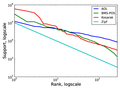
Figure 3: The distribution of 300 highest scores from experiment datasets.

Datasets. The performance of different algorithms would be affected by the distribution of query scores, we thus want to evaluate the algorithms on several representative distributions. In the experiments, we use the item frequencies in three real datasets: BMS-POS, Kosarak and AOL as representative distributions of query scores. In addition, we also use the distribution inspired by the Zipf’s law, which states that given some corpus of natural language utterances, the frequency of any word is inversely proportional to its rank in the frequency table. Similar phenomenon occurs in many other rankings unrelated to language, such as the population ranks of cities in various countries, corporation sizes, income rankings, ranks of number of people watching the same TV channel, and so on. In this distribution, the i𝑖i’th query has a score proportional to 1i1𝑖\frac{1}{i}. The characteristics of these datasets are summarized in Table 1, and the distribution of the 300300300 highest scores are shown in Figure 3.

Refer to caption
Refer to caption Refer to caption
(a) BMS-POS, SER (b) BMS-POS, FNR
Refer to caption Refer to caption
(c) Kosarak, SER (d) Kosarak, FNR
Refer to caption Refer to caption
(e) AOL, SER (f) AOL, FNR
Refer to caption Refer to caption
(g) Zipf Synthe, SER (h) Zipf Synthe, FNR
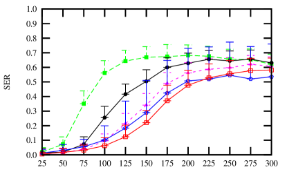
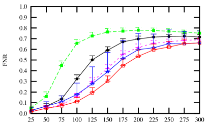
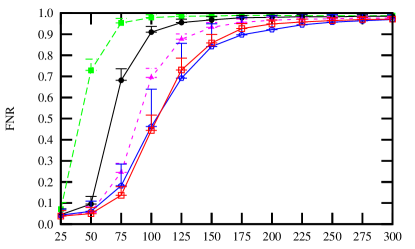
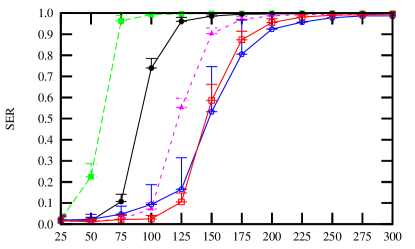
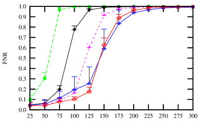
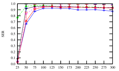
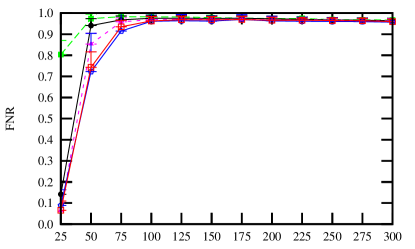
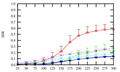
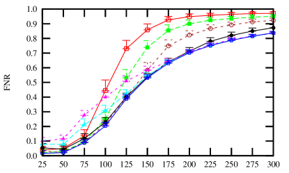
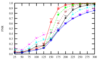
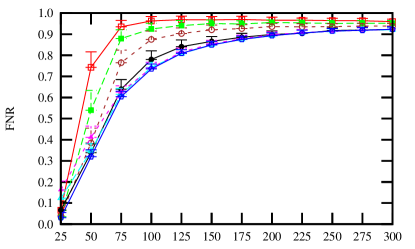
Figure 4: Comparison of interactive approaches: SVT-DPBook and SVT-S with different budget allocation. Privacy budget ϵ=0.1italic-ϵ0.1\epsilon=0.1. x-axis: top-c𝑐c
Refer to caption
Refer to caption Refer to caption
(a) BMS-POS, SER (b) BMS-POS, FNR
Refer to caption Refer to caption
(c) Kosarak, SER (d) Kosarak, FNR
Refer to caption Refer to caption
(e) AOL, SER (f) AOL, FNR
Refer to caption Refer to caption
(g) Zipf Synthe, SER (h) Zipf Synthe, FNR
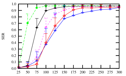
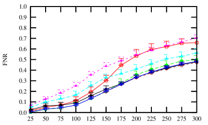
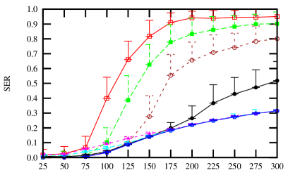
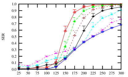
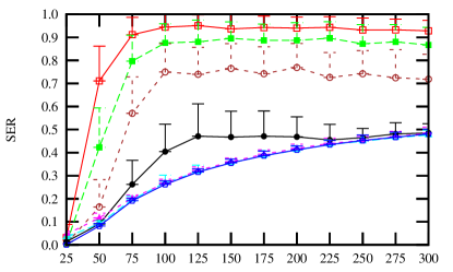
Figure 5: Comparison of non-interactive approaches: EM and SVT-ReTr with different thresholds. Privacy budget ϵ=0.1italic-ϵ0.1\epsilon=0.1. x-axis: top-c𝑐c.

Evaluation Setup. We consider the following algorithms. SVT-DPBook is from Dwork and Roth’s 2014 book [8] (Alg. 2). SVT-S is our proposed standard SVT, i.e., Alg. 7 without numerical outputs (ϵ3=0subscriptitalic-ϵ30\epsilon_{3}=0); and since the count query is monotonic, we use the version for monotonic queries in Section 4.3. We consider four privacy budget allocations, 1:1, 1:3, 1:c𝑐c and 1:c2/3superscript𝑐23c^{2/3}, where the last is what our analysis suggests for the monotonic case. These algorithms can be applied in both the interactive and the non-interactive setting.

For the non-interactive setting, we consider EM and SVT-ReTr, which is SVT with the optimizations of increasing the threshold and retraversing through the queries (items) until c𝑐c of them are selected. We fix the privacy budget allocation to be 1:c2/3:1superscript𝑐231:c^{2/3} and vary the amount we increase the threshold from 1D, 2D, \ldots, to 5D, where 1D means adding one standard deviation of the added noises to the threshold.

We vary c𝑐c from 25 to 300, and each time uses the average score for the c𝑐c’th query and the c+1𝑐1c+1’th query as the threshold. We show results for privacy budget ϵ=0.1italic-ϵ0.1\epsilon=0.1 in the paper. We omit results for other ϵitalic-ϵ\epsilon values because of space limitation. We note that varying c𝑐c have a similar impact of varying ϵitalic-ϵ\epsilon, since the accuracy of each method is mostly affect by ϵcitalic-ϵ𝑐\frac{\epsilon}{c}; therefore the impact of different ϵitalic-ϵ\epsilon can be seen from different c𝑐c values. We run each experiment 100 times, each time randomizing the order of items to be examined. We report the average and standard deviation of SER. All algorithms are implemented in Python 2.7 and all the experiments are conducted on an Intel Core i7-3770 3.40GHz PC with 16GB memory.

Results in the Interactive Setting. Figure 4 reports the results for the algorithms that can be applied in the interactive setting. While it is clear that in some settings (such as when c=25𝑐25c=25) all methods are quite accurate, and in some other settings all methods are very inaccurate (such as when c100𝑐100c\geq 100 for the Zipf dataset), in the settings in between the two extremes, the differences between these methods are quite large.

SVT-DPBook performs the worst, followed by SVT-S-1:1, then by SVT-S-1:3, and finally by SVT-S-1:c and SVT-S-1:c23. The differences among these algorithms can be quite pronounced. For example, on the Kosarak dataset, with ϵ=0.1italic-ϵ0.1\epsilon=0.1, c=50𝑐50c=50, SVT-DPBook’s SER is 0.7050.7050.705, which means that the average support of selected items is only around 30%percent3030\% of that for the true top-505050 items, which we interpret to mean that the output is meaningless. In contrast, all four SVT-S algorithms have SER less than 0.05, suggesting high accuracy in the selection. SVT-DPBook’s poor performance is due to the fact that the threshold is perturbed by a noise with scale as large as cΔ/ϵ𝑐Δitalic-ϵc\Delta/\epsilon.

For the differences among the four budget allocation approaches, it appears that the performance of 1:c:1𝑐1:c and 1:c23:1superscript𝑐231:c^{\frac{2}{3}} are clearly better than the others; and their advantages over the standard 1:1:111:1 allocation is quite pronounced. Which of 1:c:1𝑐1:c and 1:c23:1superscript𝑐231:c^{\frac{2}{3}} is better is less clear. In general, the former is better for larger c𝑐c values, where the error is higher, and the latter is better for smaller c𝑐c values, where the error is lower. Also note that 1:c:1𝑐1:c results in a significantly larger standard deviation. For these reasons, we interpret the results as supporting the recommendation of using 1:c2/3superscript𝑐23c^{2/3} budget allocation.

Results in the Non-interactive Setting. Figure 5 reports the results for the algorithms that can be applied in the noninteractive setting. We observe that EM clearly performs better than SVT-ReTr-1:c23, which performs essentially the same as SVT-S-1:c23, which is the best algorithm for the interactive case, and is already much better than SVT algorithms used in the literature. For example, for the AOL dataset with c=150𝑐150c=150, EM’s SER is 0.150.150.15, while SVT-S with 1:c2/3:1superscript𝑐231:c^{2/3} allocation has SER of 0.590.590.59, and SVT-S with 1:1:111:1 allocation has SER of 0.990.990.99.

It is interesting to see that increasing the threshold can significantly improve the accuracy of SVT with Retraversal. However, the best threshold increment value depends on the dataset and the number of items to be selected. For example, 5D works well for Zipf, and for Kosarak and AOL when c𝑐c is large, but works not as well for BMS and for Kosarak and AOL when c𝑐c is small. Since it is unclear how to select the best threshold increment value, and even with the best threshold increment, SVT-ReTr performs no better than EM, our experiments suggest that usage of SVT should be replaced by EM in the non-interactive setting.

7 Related Work

SVT was introduced by Dwork et al. [7], and improved by Roth and Roughgarden [16] and by Hardt and Rothblum [12]. These usages are in an interactive setting. An early description of SVT as a stand-alone technique appeared in Roth’s 2011 lecture notes [15], which is Alg. 3 in this paper, and is in fact \infty-DP. The algorithms in [16, 12] also has another difference, as discussed in Section 3.4. Another version of SVT appeared in the 2014 book [8], which is Alg. 2. This version is used in some papers, e.g., [17]. We show that it is possible to add less noise and obtain higher accuracy for the same privacy parameter.

Lee and Clifton [13] used a variant of SVT (see Algorithm 4) to find itemsets whose support is above the threshold. Stoddard et al. [18] proposed another variant (see Algorithm 5) for private feature selection for classification to pick out the set of features with scores greater than the perturbed threshold. Chen et al. [1] employed yet another variant of SVT (see Algorithm 6) to return attribute pairs with mutual information greater than the corresponding noisy threshold. These usages are not private. Some of these errors were pointed in [2], in which a generalized private threshold testing algorithm (GPTT) that attempts to model the SVT variants in [13, 18, 1] was introduced. The authors showed that GPTT did not satisfy ϵsuperscriptitalic-ϵ\epsilon^{\prime}-DP for any finite ϵsuperscriptitalic-ϵ\epsilon^{\prime}. But there is an error in the proof, as shown in Section 3.3. Independent from our work, Zhang et al. [20] presented two proofs that the variant of SVT violates DP without discussing the cause of the errors. Also presented in [20] is a special case of our proposed Alg. 1 for counting queries. To our knowledge, the general version of our improved SVT (Alg. 1 and Alg. 7), the techniques of optimizing budget allocation, the technique of using re-traversal to improve SVT, and the comparison of SVT and EM are new in our work.

8 Conclusion

We have introduced a new version of SVT that provides better utility. We also introduce an effective technique to improve the performance of SVT by optimizing the distribution of privacy budget. These enhancements achieve better utility than the state of the art SVT and can be applied to improve utility in the interactive setting. We have also explained the misunderstandings and errors in a number of papers that use or analyze SVT; and believe that these will help clarify the misunderstandings regarding SVT and help avoid similar errors in the future. We have also shown that in the non-interactive setting, EM should be preferred over SVT.

References

  • [1] R. Chen, Q. Xiao, Y. Zhang, and J. Xu. Differentially private high-dimensional data publication via sampling-based inference. In KDD, pages 129–138, 2015.
  • [2] Y. Chen and A. Machanavajjhala. On the privacy properties of variants on the sparse vector technique. CoRR, abs/1508.07306, 2015.
  • [3] I. Dinur and K. Nissim. Revealing information while preserving privacy. In PODS, pages 202–210, 2003.
  • [4] C. Dwork. Differential privacy. In ICALP, pages 1–12, 2006.
  • [5] C. Dwork, F. McSherry, K. Nissim, and A. Smith. Calibrating noise to sensitivity in private data analysis. In TCC, pages 265–284, 2006.
  • [6] C. Dwork, F. McSherry, and K. Talwar. The price of privacy and the limits of LP decoding. In STOC, pages 85–94, 2007.
  • [7] C. Dwork, M. Naor, O. Reingold, G. Rothblum, and S. Vadhan. On the complexity of differentially private data release: efficient algorithms and hardness results. STOC, pages 381–390, 2009.
  • [8] C. Dwork and A. Roth. The algorithmic foundations of differential privacy. Theoretical Computer Science, 9(3-4):211–407, 2013.
  • [9] C. Dwork, G. N. Rothblum, and S. Vadhan. Boosting and differential privacy. FOCS ’10, pages 51–60, 2010.
  • [10] C. Dwork and S. Yekhanin. New efficient attacks on statistical disclosure control mechanisms. CRYPTO’08, pages 469–480, 2008.
  • [11] A. Gupta, A. Roth, and J. Ullman. Iterative constructions and private data release. In TCC, pages 339–356, 2012.
  • [12] M. Hardt and G. N. Rothblum. A multiplicative weights mechanism for privacy-preserving data analysis. In FOCS, pages 61–70, 2010.
  • [13] J. Lee and C. W. Clifton. Top-k frequent itemsets via differentially private fp-trees. In KDD ’14, pages 931–940, 2014.
  • [14] F. McSherry and K. Talwar. Mechanism design via differential privacy. In FOCS, pages 94–103, 2007.
  • [15] A. Roth. The sparse vector technique, 2011. Lecture notes for “ The Algorithmic Foundations of Data Privacy”.
  • [16] A. Roth and T. Roughgarden. Interactive privacy via the median mechanism. In STOC, pages 765–774, 2010.
  • [17] R. Shokri and V. Shmatikov. Privacy-preserving deep learning. In CCS, pages 1310–1321, 2015.
  • [18] B. Stoddard, Y. Chen, and A. Machanavajjhala. Differentially private algorithms for empirical machine learning. CoRR, abs/1411.5428, 2014.
  • [19] J. Zhang, G. Cormode, C. M. Procopiuc, D. Srivastava, and X. Xiao. Privbayes: Private data release via bayesian networks. In SIGMOD ’14, pages 1423–1434, 2014.
  • [20] J. Zhang, X. Xiao, and X. Xie. Privtree: A differentially private algorithm for hierarchical decompositions. SIGMOD ’16, pages 155–170, 2016.

9 Appendix

9.1 Proof that Alg. 3 is non-private

Theorem 9.11.

Alg. 3 is not ϵsuperscriptitalic-ϵ\epsilon^{\prime}-DP for any finite ϵsuperscriptitalic-ϵ\epsilon^{\prime}.

Proof 9.12.

Set c=1𝑐1c=1 for simplicity. Given any finite ϵ>0superscriptitalic-ϵ0\epsilon^{\prime}>0, we construct an example to show that Alg. 3 is not ϵsuperscriptitalic-ϵ\epsilon^{\prime}-DP. Consider an example with T=0𝑇0T=0, and m+1𝑚1m+1 queries 𝐪𝐪\mathbf{q} with sensitivity ΔΔ\Delta such that 𝐪(D)=0mΔ𝐪𝐷superscript0𝑚Δ\mathbf{q}(D)=0^{m}\Delta and 𝐪(D)=Δm0𝐪superscript𝐷superscriptΔ𝑚0\mathbf{q}(D^{\prime})=\Delta^{m}0, and the output vector 𝐚=m0𝐚superscriptbottom𝑚0\mbox{\boldmath$a$}=\bot^{m}0, that is, only the last query answer is a numeric value 00. Let 𝒜𝒜\mathcal{A} be Alg. 3. We show that 𝖯𝗋[𝒜(D)=𝐚]𝖯𝗋[𝒜(D)=𝐚]eϵ𝖯𝗋delimited-[]𝒜𝐷𝐚𝖯𝗋delimited-[]𝒜superscript𝐷𝐚superscript𝑒superscriptitalic-ϵ\frac{\mathsf{Pr}\!\left[\mathcal{A}(D)=\scriptsize{\mbox{\boldmath$a$}}\right]}{\mathsf{Pr}\!\left[\mathcal{A}(D^{\prime})=\scriptsize{\mbox{\boldmath$a$}}\right]}\geq e^{\epsilon^{\prime}} for any ϵ>0superscriptitalic-ϵ0\epsilon^{\prime}>0 when m𝑚m is large enough.

We denote the cumulative distribution function of 𝖫𝖺𝗉(2Δϵ)𝖫𝖺𝗉2Δitalic-ϵ\mathsf{Lap}\left(\frac{2\Delta}{\epsilon}\right) by F(x)𝐹𝑥F(x). We have

𝖯𝗋[𝒜(D)=𝒂]𝖯𝗋delimited-[]𝒜𝐷𝒂\displaystyle\mathsf{Pr}\!\left[\mathcal{A}(D)=\mbox{\boldmath$a$}\right]
=\displaystyle= 𝖯𝗋[ρ=z]fD(z)𝖯𝗋[Δ+νm+1zΔ+νm+1=0]𝑑zsuperscriptsubscript𝖯𝗋delimited-[]𝜌𝑧subscript𝑓𝐷𝑧𝖯𝗋delimited-[]Δsubscript𝜈𝑚1𝑧Δsubscript𝜈𝑚10differential-d𝑧\displaystyle\int_{-\infty}^{\infty}\!\mathsf{Pr}\!\left[\rho\!=\!z\right]f_{D}(z)\mathsf{Pr}\!\left[\Delta\!+\!\nu_{m+1}\!\geq\!z\wedge\Delta\!+\!\nu_{m+1}\!=\!0\right]\>dz
=\displaystyle= 𝖯𝗋[ρ=z]fD(z)𝖯𝗋[0z]𝖯𝗋[νm+1=Δ]𝑑zsuperscriptsubscript𝖯𝗋delimited-[]𝜌𝑧subscript𝑓𝐷𝑧𝖯𝗋delimited-[]0𝑧𝖯𝗋delimited-[]subscript𝜈𝑚1Δdifferential-d𝑧\displaystyle\int_{-\infty}^{\infty}\mathsf{Pr}\!\left[\rho\!=\!z\right]f_{D}(z)\mathsf{Pr}\!\left[0\geq z\right]\mathsf{Pr}\!\left[\nu_{m+1}=-\Delta\right]\>dz
=\displaystyle= ϵ4Δeϵ2𝖯𝗋[ρ=z]fD(z)𝖯𝗋[0z]𝑑zitalic-ϵ4Δsuperscript𝑒italic-ϵ2superscriptsubscript𝖯𝗋delimited-[]𝜌𝑧subscript𝑓𝐷𝑧𝖯𝗋delimited-[]0𝑧differential-d𝑧\displaystyle\frac{\epsilon}{4\Delta}e^{-\frac{\epsilon}{2}}\int_{-\infty}^{\infty}\mathsf{Pr}\!\left[\rho\!=\!z\right]f_{D}(z)\mathsf{Pr}\!\left[0\geq z\right]\>dz
=\displaystyle= ϵ4Δeϵ20𝖯𝗋[ρ=z]fD(z)𝑑zitalic-ϵ4Δsuperscript𝑒italic-ϵ2superscriptsubscript0𝖯𝗋delimited-[]𝜌𝑧subscript𝑓𝐷𝑧differential-d𝑧\displaystyle\frac{\epsilon}{4\Delta}e^{-\frac{\epsilon}{2}}\int_{-\infty}^{0}\mathsf{Pr}\!\left[\rho\!=\!z\right]f_{D}(z)\>dz
=\displaystyle= ϵ4Δeϵ20𝖯𝗋[ρ=z]i=1m𝖯𝗋[νi<z]dzitalic-ϵ4Δsuperscript𝑒italic-ϵ2superscriptsubscript0𝖯𝗋delimited-[]𝜌𝑧superscriptsubscriptproduct𝑖1𝑚𝖯𝗋delimited-[]subscript𝜈𝑖𝑧𝑑𝑧\displaystyle\frac{\epsilon}{4\Delta}e^{-\frac{\epsilon}{2}}\int_{-\infty}^{0}\mathsf{Pr}\!\left[\rho=z\right]\prod\limits_{i=1}^{m}\mathsf{Pr}\!\left[\nu_{i}<z\right]\>dz
=\displaystyle= ϵ4Δeϵ20𝖯𝗋[ρ=z](F(z))m𝑑z,italic-ϵ4Δsuperscript𝑒italic-ϵ2superscriptsubscript0𝖯𝗋delimited-[]𝜌𝑧superscript𝐹𝑧𝑚differential-d𝑧\displaystyle\frac{\epsilon}{4\Delta}e^{-\frac{\epsilon}{2}}\int_{-\infty}^{0}\mathsf{Pr}\!\left[\rho=z\right](F(z))^{m}\>dz, (13)
and similarly
𝖯𝗋[𝒜(D)=𝒂]=ϵ4Δ0𝖯𝗋[ρ=z](F(zΔ))m𝑑z.𝖯𝗋delimited-[]𝒜superscript𝐷𝒂italic-ϵ4Δsuperscriptsubscript0𝖯𝗋delimited-[]𝜌superscript𝑧superscript𝐹superscript𝑧Δ𝑚differential-dsuperscript𝑧\displaystyle\mathsf{Pr}\!\left[\mathcal{A}(D^{\prime})=\mbox{\boldmath$a$}\right]=\frac{\epsilon}{4\Delta}\int_{-\infty}^{0}\mathsf{Pr}\!\left[\rho=z^{\prime}\right](F(z^{\prime}-\Delta))^{m}\>dz^{\prime}. (14)

The fact that 00 is given as an output reveals the information that the noisy threshold is at most 00, forcing the range of integration to be from -\infty to 00, instead of from -\infty to \infty. This prevents the use of changing z𝑧z in (13) to zΔsuperscript𝑧Δz^{\prime}-\Delta to bound the ratio of (13) to (14).

Noting that F(z)F(zΔ)=eϵ2𝐹𝑧𝐹𝑧Δsuperscript𝑒italic-ϵ2\frac{F(z)}{F(z-\Delta)}=e^{\frac{\epsilon}{2}} for any z0𝑧0z\leq 0, we thus have

𝖯𝗋[𝒜(D)=𝒂]𝖯𝗋[𝒜(D)=𝒂]𝖯𝗋delimited-[]𝒜𝐷𝒂𝖯𝗋delimited-[]𝒜superscript𝐷𝒂\displaystyle\frac{\mathsf{Pr}\!\left[\mathcal{A}(D)=\mbox{\boldmath$a$}\right]}{\mathsf{Pr}\!\left[\mathcal{A}(D^{\prime})=\mbox{\boldmath$a$}\right]} =eϵ20𝖯𝗋[ρ=z](F(z))m𝑑z0𝖯𝗋[ρ=z](F(zΔ))m𝑑zabsentsuperscript𝑒italic-ϵ2superscriptsubscript0𝖯𝗋delimited-[]𝜌𝑧superscript𝐹𝑧𝑚differential-d𝑧superscriptsubscript0𝖯𝗋delimited-[]𝜌superscript𝑧superscript𝐹superscript𝑧Δ𝑚differential-dsuperscript𝑧\displaystyle=e^{-\frac{\epsilon}{2}}\frac{\int_{-\infty}^{0}\mathsf{Pr}\!\left[\rho=z\right](F(z))^{m}\>dz}{\int_{-\infty}^{0}\mathsf{Pr}\!\left[\rho=z^{\prime}\right](F(z^{\prime}-\Delta))^{m}\>dz^{\prime}}
=eϵ20𝖯𝗋[ρ=z](eϵ2F(zΔ))m𝑑z0𝖯𝗋[ρ=z](F(zΔ))m𝑑zabsentsuperscript𝑒italic-ϵ2superscriptsubscript0𝖯𝗋delimited-[]𝜌𝑧superscriptsuperscript𝑒italic-ϵ2𝐹𝑧Δ𝑚differential-d𝑧superscriptsubscript0𝖯𝗋delimited-[]𝜌superscript𝑧superscript𝐹superscript𝑧Δ𝑚differential-dsuperscript𝑧\displaystyle=e^{-\frac{\epsilon}{2}}\frac{\int_{-\infty}^{0}\mathsf{Pr}\!\left[\rho=z\right](e^{\frac{\epsilon}{2}}F(z-\Delta))^{m}\>dz}{\int_{-\infty}^{0}\mathsf{Pr}\!\left[\rho=z^{\prime}\right](F(z^{\prime}-\Delta))^{m}\>dz^{\prime}}
=e(m1)ϵ2,absentsuperscript𝑒𝑚1italic-ϵ2\displaystyle=e^{(m-1)\frac{\epsilon}{2}},

and thus when m>2ϵϵ+1𝑚2superscriptitalic-ϵitalic-ϵ1m>\lceil\frac{2\epsilon^{\prime}}{\epsilon}\rceil+1, we have 𝖯𝗋[𝒜(D)=𝐚]𝖯𝗋[𝒜(D)=𝐚]>eϵ𝖯𝗋delimited-[]𝒜𝐷𝐚𝖯𝗋delimited-[]𝒜superscript𝐷𝐚superscript𝑒superscriptitalic-ϵ\frac{\mathsf{Pr}\!\left[\mathcal{A}(D)=\scriptsize{\mbox{\boldmath$a$}}\right]}{\mathsf{Pr}\!\left[\mathcal{A}(D^{\prime})=\scriptsize{\mbox{\boldmath$a$}}\right]}>e^{\epsilon^{\prime}}.

9.2 Proof that Alg. 6 is non-private

Theorem 9.13.

Alg. 6 is not ϵsuperscriptitalic-ϵ\epsilon^{\prime}-DP for any finite ϵsuperscriptitalic-ϵ\epsilon^{\prime}.

Proof 9.14.

We construct a counterexample with Δ=1Δ1\Delta=1, T=0𝑇0T=0, and 2m2𝑚2m queries such that 𝐪(D)=02m𝐪𝐷superscript02𝑚\mathbf{q}(D)=0^{2m}, and 𝐪(D)=1m(1)m𝐪superscript𝐷superscript1𝑚superscript1𝑚\mathbf{q}(D^{\prime})=1^{m}(-1)^{m}. Consider the output vector 𝐚=mm\mbox{\boldmath$a$}=\bot^{m}\top^{m}. Denote the cumulative distribution function of νisubscript𝜈𝑖\nu_{i} by F(x)𝐹𝑥F(x). From Eq. (5), we have

𝖯𝗋[𝒜(D)=𝒂]𝖯𝗋delimited-[]𝒜𝐷𝒂\displaystyle\mathsf{Pr}\!\left[\mathcal{A}(D)=\mbox{\boldmath$a$}\right]
=𝖯𝗋[ρ=z]i=1m𝖯𝗋[0+νi<z]i=m+12m𝖯𝗋[0+νiz]dzabsentsuperscriptsubscript𝖯𝗋delimited-[]𝜌𝑧superscriptsubscriptproduct𝑖1𝑚𝖯𝗋delimited-[]0subscript𝜈𝑖𝑧superscriptsubscriptproduct𝑖𝑚12𝑚𝖯𝗋delimited-[]0subscript𝜈𝑖𝑧𝑑𝑧\displaystyle=\int_{-\infty}^{\infty}\mathsf{Pr}\!\left[\rho=z\right]\prod\limits_{i=1}^{m}\mathsf{Pr}\!\left[0\!+\!\nu_{i}<z\right]\prod\limits_{i=m+1}^{2m}\mathsf{Pr}\!\left[0\!+\!\nu_{i}\geq z\right]\>dz
=𝖯𝗋[ρ=z](F(z)(1F(z)))m𝑑z,absentsuperscriptsubscript𝖯𝗋delimited-[]𝜌𝑧superscript𝐹𝑧1𝐹𝑧𝑚differential-d𝑧\displaystyle=\int_{-\infty}^{\infty}\mathsf{Pr}\!\left[\rho=z\right](F(z)(1-F(z)))^{m}\>dz,

and

𝖯𝗋[𝒜(D)=𝒂]𝖯𝗋delimited-[]𝒜superscript𝐷𝒂\displaystyle\mathsf{Pr}\!\left[\mathcal{A}(D^{\prime})=\mbox{\boldmath$a$}\right]
=𝖯𝗋[ρ=z]i=1m𝖯𝗋[1+νi<z]i=m+12m𝖯𝗋[1+νiz]dzabsentsuperscriptsubscript𝖯𝗋delimited-[]𝜌𝑧superscriptsubscriptproduct𝑖1𝑚𝖯𝗋delimited-[]1subscript𝜈𝑖𝑧superscriptsubscriptproduct𝑖𝑚12𝑚𝖯𝗋delimited-[]1subscript𝜈𝑖𝑧𝑑𝑧\displaystyle=\int_{-\infty}^{\infty}\mathsf{Pr}\!\left[\rho=z\right]\prod\limits_{i=1}^{m}\mathsf{Pr}\!\left[1\!+\!\nu_{i}<z\right]\prod\limits_{i=m+1}^{2m}\mathsf{Pr}\!\left[-1\!+\!\nu_{i}\geq z\right]\>dz
=𝖯𝗋[ρ=z](F(z1)(1F(z+1)))m𝑑z.absentsuperscriptsubscript𝖯𝗋delimited-[]𝜌𝑧superscript𝐹𝑧11𝐹𝑧1𝑚differential-d𝑧\displaystyle=\int_{-\infty}^{\infty}\mathsf{Pr}\!\left[\rho=z\right](F(z-1)(1-F(z\!+\!1)))^{m}\>dz.

We now show that 𝖯𝗋[𝒜(D)=𝐚]𝖯𝗋[𝒜(D)=𝐚]𝖯𝗋delimited-[]𝒜𝐷𝐚𝖯𝗋delimited-[]𝒜superscript𝐷𝐚\frac{\mathsf{Pr}\!\left[\mathcal{A}(D)=\scriptsize{\mbox{\boldmath$a$}}\right]}{\mathsf{Pr}\!\left[\mathcal{A}(D^{\prime})=\scriptsize{\mbox{\boldmath$a$}}\right]} is unbounded as m𝑚m increases, proving this theorem. Compare F(z)(1F(z))𝐹𝑧1𝐹𝑧F(z)(1-F(z)) with F(z1)(1F(z+1))𝐹𝑧11𝐹𝑧1F(z-1)(1-F(z\!+\!1)). Note that F(z)𝐹𝑧F(z) is monotonically increasing. When z0𝑧0z\leq 0,

F(z)(1F(z))F(z1)(1F(z+1))F(z)F(z1)=12eϵ2z12eϵ2(z1)=eϵ2.𝐹𝑧1𝐹𝑧𝐹𝑧11𝐹𝑧1𝐹𝑧𝐹𝑧112superscript𝑒italic-ϵ2𝑧12superscript𝑒italic-ϵ2𝑧1superscript𝑒italic-ϵ2\frac{F(z)(1-F(z))}{F(z-1)(1-F(z\!+\!1))}\geq\frac{F(z)}{F(z-1)}=\frac{\frac{1}{2}e^{\frac{\epsilon}{2}z}}{\frac{1}{2}e^{\frac{\epsilon}{2}(z-1)}}=e^{\frac{\epsilon}{2}}.

When z>0𝑧0z>0, we also have

F(z)(1F(z))F(z1)(1F(z+1))1F(z)1F(z+1)=12eϵ2z12eϵ2(z+1)=eϵ2.𝐹𝑧1𝐹𝑧𝐹𝑧11𝐹𝑧11𝐹𝑧1𝐹𝑧112superscript𝑒italic-ϵ2𝑧12superscript𝑒italic-ϵ2𝑧1superscript𝑒italic-ϵ2\frac{F(z)(1-F(z))}{F(z-1)(1-F(z\!+\!1))}\geq\frac{1-F(z)}{1-F(z+1)}=\frac{\frac{1}{2}e^{-\frac{\epsilon}{2}z}}{\frac{1}{2}e^{-\frac{\epsilon}{2}(z+1)}}=e^{\frac{\epsilon}{2}}.

So, 𝖯𝗋[𝒜(D)=𝐚]𝖯𝗋[𝒜(D)=𝐚]emϵ2𝖯𝗋delimited-[]𝒜𝐷𝐚𝖯𝗋delimited-[]𝒜superscript𝐷𝐚superscript𝑒𝑚italic-ϵ2\frac{\mathsf{Pr}\!\left[\mathcal{A}(D)=\scriptsize{\mbox{\boldmath$a$}}\right]}{\mathsf{Pr}\!\left[\mathcal{A}(D^{\prime})=\scriptsize{\mbox{\boldmath$a$}}\right]}\geq e^{\frac{m\epsilon}{2}}, which is greater than eϵsuperscript𝑒superscriptitalic-ϵe^{\epsilon^{\prime}} when m>2ϵϵ𝑚2superscriptitalic-ϵitalic-ϵm>\lceil\frac{2\epsilon^{\prime}}{\epsilon}\rceil for any finite ϵsuperscriptitalic-ϵ\epsilon^{\prime}.

9.3 Error of non-privacy proof in [2]

The proof in [2] that GPTT is non-private considers the counter-example with Δ=1Δ1\Delta=1, T=0𝑇0T=0, a sequence 𝐪𝐪\mathbf{q} of 2t2𝑡2t queries such that 𝐪(D)=0t1t𝐪𝐷superscript0𝑡superscript1𝑡\mathbf{q}(D)=0^{t}1^{t} and 𝐪(D)=1t0t𝐪superscript𝐷superscript1𝑡superscript0𝑡\mathbf{q}(D^{\prime})=1^{t}0^{t}, and the output vector 𝒂=tt\mbox{\boldmath$a$}=\bot^{t}\top^{t}. Then

𝖯𝗋[𝖦𝖯𝖳𝖳(D)=𝒂]𝖯𝗋[𝖦𝖯𝖳𝖳(D)=𝒂]𝖯𝗋delimited-[]𝖦𝖯𝖳𝖳𝐷𝒂𝖯𝗋delimited-[]𝖦𝖯𝖳𝖳superscript𝐷𝒂\displaystyle\frac{\mathsf{Pr}\!\left[\mathsf{GPTT}(D)=\mbox{\boldmath$a$}\right]}{\mathsf{Pr}\!\left[\mathsf{GPTT}(D^{\prime})=\mbox{\boldmath$a$}\right]} =𝖯𝗋[ρ=z](Fϵ2(z)Fϵ2(z)Fϵ2(z1))t𝑑z𝖯𝗋[ρ=z](Fϵ2(z1)Fϵ2(z)Fϵ2(z1))t𝑑zabsentsuperscriptsubscript𝖯𝗋delimited-[]𝜌𝑧superscriptsubscript𝐹subscriptitalic-ϵ2𝑧subscript𝐹subscriptitalic-ϵ2𝑧subscript𝐹subscriptitalic-ϵ2𝑧1𝑡differential-d𝑧superscriptsubscript𝖯𝗋delimited-[]𝜌𝑧superscriptsubscript𝐹subscriptitalic-ϵ2𝑧1subscript𝐹subscriptitalic-ϵ2𝑧subscript𝐹subscriptitalic-ϵ2𝑧1𝑡differential-d𝑧\displaystyle=\frac{\int_{\!-\!\infty}^{\infty}\mathsf{Pr}\!\left[\rho=z\right]\left(F_{\epsilon_{2}}(z)\!-\!F_{\epsilon_{2}}(z)F_{\epsilon_{2}}(z\!-\!1)\right)^{t}dz}{\int_{-\infty}^{\infty}\mathsf{Pr}\!\left[\rho=z\right]\left(F_{\epsilon_{2}}(z\!-\!1)\!-\!F_{\epsilon_{2}}(z)F_{\epsilon_{2}}(z\!-\!1)\right)^{t}dz}
whereFϵ(x)wheresubscript𝐹italic-ϵ𝑥\displaystyle{\small\mbox{where}\;\;F_{\epsilon}(x)} is the cumulative distribution function of 𝖫𝖺𝗉(1/ϵ).is the cumulative distribution function of 𝖫𝖺𝗉1italic-ϵ\displaystyle{\small\mbox{ is the cumulative distribution function of }\mathsf{Lap}\left(1/\epsilon\right).}

The goal of the proof is to show that the above is unbounded as t𝑡t increases. A key observation is that the ratio of the integrands of the two integrals is always larger than 111, i.e.,

κ(z)=Fϵ2(z)Fϵ2(z)Fϵ2(z1)Fϵ2(z1)Fϵ2(z)Fϵ2(z1)>1𝜅𝑧subscript𝐹subscriptitalic-ϵ2𝑧subscript𝐹subscriptitalic-ϵ2𝑧subscript𝐹subscriptitalic-ϵ2𝑧1subscript𝐹subscriptitalic-ϵ2𝑧1subscript𝐹subscriptitalic-ϵ2𝑧subscript𝐹subscriptitalic-ϵ2𝑧11\kappa(z)=\frac{F_{\epsilon_{2}}(z)-F_{\epsilon_{2}}(z)F_{\epsilon_{2}}(z-1)}{F_{\epsilon_{2}}(z-1)-F_{\epsilon_{2}}(z)F_{\epsilon_{2}}(z-1)}>1

For example, since Fϵ(x)subscript𝐹italic-ϵ𝑥F_{\epsilon}(x) is the cumulative distribution function of 𝖫𝖺𝗉(1/ϵ)𝖫𝖺𝗉1italic-ϵ\mathsf{Lap}\left(1/\epsilon\right), we have Fϵ2(0)=1/2subscript𝐹subscriptitalic-ϵ2012F_{\epsilon_{2}}(0)=1/2 and Fϵ2(1)<1/2subscript𝐹subscriptitalic-ϵ2112F_{\epsilon_{2}}(-1)<1/2; and thus κ(0)=1Fϵ2(1)Fϵ2(1)>1𝜅01subscript𝐹subscriptitalic-ϵ21subscript𝐹subscriptitalic-ϵ211\kappa(0)=\frac{1-F_{\epsilon_{2}}(-1)}{F_{\epsilon_{2}}(-1)}>1. However, when |z|𝑧|z| goes to \infty, κ(z)𝜅𝑧\kappa(z) goes to 111. Thus the proof tries to limit the integrals to be a finite interval so that there is a lower-bound for κ(z)𝜅𝑧\kappa(z) that is greater than 111. It denotes α=𝖯𝗋[𝖦𝖯𝖳𝖳(D)=𝒂]𝛼𝖯𝗋delimited-[]𝖦𝖯𝖳𝖳superscript𝐷𝒂\alpha=\mathsf{Pr}\!\left[\mathsf{GPTT}(D^{\prime})=\mbox{\boldmath$a$}\right]. Then choose parameter δ=|Fϵ11(α4)|𝛿superscriptsubscript𝐹subscriptitalic-ϵ11𝛼4\delta=|F_{\epsilon_{1}}^{-1}(\frac{\alpha}{4})| to use [δ,δ]𝛿𝛿[-\delta,\delta] as the finite interval, and thus

α2δδ𝖯𝗋[ρ=z](Fϵ2(z1)Fϵ2(z)Fϵ2(z1))t𝑑z.𝛼2superscriptsubscript𝛿𝛿𝖯𝗋delimited-[]𝜌𝑧superscriptsubscript𝐹subscriptitalic-ϵ2𝑧1subscript𝐹subscriptitalic-ϵ2𝑧subscript𝐹subscriptitalic-ϵ2𝑧1𝑡differential-d𝑧\displaystyle\alpha\leq 2\int_{-\delta}^{\delta}\mathsf{Pr}\!\left[\rho=z\right]\left(F_{\epsilon_{2}}(z-1)-F_{\epsilon_{2}}(z)F_{\epsilon_{2}}(z-1)\right)^{t}dz.

Denote the minimum of κ(z)𝜅𝑧\kappa(z) in the closed interval [δ,δ]𝛿𝛿[-\delta,\delta] by κ𝜅\kappa. Then we have 𝖯𝗋[𝖦𝖯𝖳𝖳(D)=𝒂]𝖯𝗋[𝖦𝖯𝖳𝖳(D)=𝒂]>κt2𝖯𝗋delimited-[]𝖦𝖯𝖳𝖳𝐷𝒂𝖯𝗋delimited-[]𝖦𝖯𝖳𝖳superscript𝐷𝒂superscript𝜅𝑡2\frac{\mathsf{Pr}\!\left[\mathsf{GPTT}(D)=\mbox{\boldmath$a$}\right]}{\mathsf{Pr}\!\left[\mathsf{GPTT}(D^{\prime})=\mbox{\boldmath$a$}\right]}>\frac{\kappa^{t}}{2}. The proof claims that for any ϵ>1superscriptitalic-ϵ1\epsilon^{\prime}>1 there exists a t𝑡t to make the above ratio larger than eϵsuperscript𝑒superscriptitalic-ϵe^{\epsilon^{\prime}}.

The proof is incorrect because of dependency in the parameters. First, α𝛼\alpha is a function of t𝑡t; and when t𝑡t increases, α𝛼\alpha decreases because the integrand above is positive and decreasing. Second, δ𝛿\delta depends on α𝛼\alpha, and when α𝛼\alpha decreases, δ𝛿\delta increases. Thus when t𝑡t increases, δ𝛿\delta increases. We write δ𝛿\delta as δ(t)𝛿𝑡\delta(t) to make the dependency on t𝑡t explicit. Third, κ𝜅\kappa, the minimum value of κ(z)𝜅𝑧\kappa(z) over the interval [δ(t),δ(t)]𝛿𝑡𝛿𝑡[-\delta(t),\delta(t)], decreases when t𝑡t increases. That is, κ𝜅\kappa is also dependent on t𝑡t, denoted by κ(t)𝜅𝑡\kappa(t), and decreases while t𝑡t increases. It is not sure that there exists such a t𝑡t that κ(t)t2>eϵ𝜅superscript𝑡𝑡2superscript𝑒superscriptitalic-ϵ\frac{\kappa(t)^{t}}{2}>e^{\epsilon^{\prime}} for any ϵ>1superscriptitalic-ϵ1\epsilon^{\prime}>1.

To demonstrate that the error in the proof cannot be easily fixed, we point out that following the logic of that proof, one can prove that Alg. 1 is not ϵsuperscriptitalic-ϵ\epsilon^{\prime}-DP for any finite ϵsuperscriptitalic-ϵ\epsilon^{\prime}. We now show such a “proof” that contradicts Lemma 1. Let 𝒜𝒜\mathcal{A} be Alg. 1, with c=1𝑐1c=1. Consider an example with Δ=1Δ1\Delta=1, T=0𝑇0T=0, a sequence 𝐪𝐪\mathbf{q} of t𝑡t queries such that 𝐪(D)=0t𝐪𝐷superscript0𝑡\mathbf{q}(D)=0^{t} and 𝐪(D)=1t𝐪superscript𝐷superscript1𝑡\mathbf{q}(D^{\prime})=1^{t}, and output vector 𝒂=t𝒂superscriptbottom𝑡\mbox{\boldmath$a$}=\bot^{t}. Let

β=𝖯𝗋[𝒜(D)=]=𝖯𝗋[ρ=z](Fϵ4(z))t𝑑z𝛽𝖯𝗋delimited-[]𝒜𝐷superscriptbottomsuperscriptsubscript𝖯𝗋delimited-[]𝜌𝑧superscriptsubscript𝐹italic-ϵ4𝑧𝑡differential-d𝑧\displaystyle\beta=\mathsf{Pr}\!\left[\mathcal{A}(D)=\bot^{\ell}\right]=\int_{-\infty}^{\infty}\mathsf{Pr}\!\left[\rho=z\right]\left(F_{\frac{\epsilon}{4}}(z)\right)^{t}dz
α=𝖯𝗋[𝒜(D)=]=𝖯𝗋[ρ=z](Fϵ4(z1))t𝑑z,𝛼𝖯𝗋delimited-[]𝒜superscript𝐷superscriptbottomsuperscriptsubscript𝖯𝗋delimited-[]𝜌𝑧superscriptsubscript𝐹italic-ϵ4𝑧1𝑡differential-d𝑧\displaystyle\alpha=\mathsf{Pr}\!\left[\mathcal{A}(D^{\prime})=\bot^{\ell}\right]=\int_{-\infty}^{\infty}\mathsf{Pr}\!\left[\rho=z\right]\left(F_{\frac{\epsilon}{4}}(z-1)\right)^{t}dz,
where Fϵ4(x) is the cumulative distribution function of 𝖫𝖺𝗉(4ϵ).where subscript𝐹italic-ϵ4𝑥 is the cumulative distribution function of 𝖫𝖺𝗉4italic-ϵ\displaystyle\quad\mbox{where }\;\;F_{\frac{\epsilon}{4}}(x)\mbox{ is the cumulative distribution function of }\mathsf{Lap}\left(\frac{4}{\epsilon}\right).

Find a parameter δ𝛿\delta such that δδ𝖯𝗋[ρ=z]𝑑z1α2superscriptsubscript𝛿𝛿𝖯𝗋delimited-[]𝜌𝑧differential-d𝑧1𝛼2\int_{-\delta}^{\delta}\mathsf{Pr}\!\left[\rho=z\right]\>dz\geq 1-\frac{\alpha}{2}. Then δδ𝖯𝗋[ρ=z](Fϵ4(z1))t𝑑zα2superscriptsubscript𝛿𝛿𝖯𝗋delimited-[]𝜌𝑧superscriptsubscript𝐹italic-ϵ4𝑧1𝑡differential-d𝑧𝛼2\int_{-\delta}^{\delta}\mathsf{Pr}\!\left[\rho=z\right]\left(F_{\frac{\epsilon}{4}}(z-1)\right)^{t}dz\geq\frac{\alpha}{2}. Let κ𝜅\kappa be the minimum value of Fϵ4(z)Fϵ4(z1)subscript𝐹italic-ϵ4𝑧subscript𝐹italic-ϵ4𝑧1\frac{F_{\frac{\epsilon}{4}}(z)}{F_{\frac{\epsilon}{4}}(z-1)} in [δ,δ]𝛿𝛿[-\delta,\delta]; it must be that κ>1𝜅1\kappa>1. Then

β𝛽\displaystyle\beta >δδ𝖯𝗋[ρ=z](Fϵ4(z))t𝑑zδδ𝖯𝗋[ρ=z](κFϵ4(z1))t𝑑zabsentsuperscriptsubscript𝛿𝛿𝖯𝗋delimited-[]𝜌𝑧superscriptsubscript𝐹italic-ϵ4𝑧𝑡differential-d𝑧superscriptsubscript𝛿𝛿𝖯𝗋delimited-[]𝜌𝑧superscript𝜅subscript𝐹italic-ϵ4𝑧1𝑡differential-d𝑧\displaystyle>\int_{-\delta}^{\delta}\mathsf{Pr}\!\left[\rho=z\right]\left(F_{\frac{\epsilon}{4}}(z)\right)^{t}dz\geq\int_{-\delta}^{\delta}\mathsf{Pr}\!\left[\rho=z\right]\left(\kappa F_{\frac{\epsilon}{4}}(z-1)\right)^{t}dz
=κtδδ𝖯𝗋[ρ=z](Fϵ4(z1))t𝑑zκt2α.absentsuperscript𝜅𝑡superscriptsubscript𝛿𝛿𝖯𝗋delimited-[]𝜌𝑧superscriptsubscript𝐹italic-ϵ4𝑧1𝑡differential-d𝑧superscript𝜅𝑡2𝛼\displaystyle=\kappa^{t}\int_{-\delta}^{\delta}\mathsf{Pr}\!\left[\rho=z\right]\left(F_{\frac{\epsilon}{4}}(z-1)\right)^{t}dz\geq\frac{\kappa^{t}}{2}\alpha.

Since κ>1𝜅1\kappa>1, one can choose a large enough t𝑡t to make βα=κt2𝛽𝛼superscript𝜅𝑡2\frac{\beta}{\alpha}=\frac{\kappa^{t}}{2} to be as large as needed. We note that this contradicts Lemma 1. The contradiction shows that the proof logic used in [2] is incorrect.