Laboratoire J. A. Dieudonné, Université Nice Sophia Antipolis, CNRS, UMR 7351 - Nice 06108, France
Chaos in fluid dynamics Polymers and polymer solutions
Elastic turbulence in a shell model of polymer solution
Abstract
We show that, at low inertia and large elasticity, shell models of viscoelastic fluids develop a chaotic behaviour with properties similar to those of elastic turbulence. The low dimensionality of shell models allows us to explore a wide range both in polymer concentration and in Weissenberg number. Our results demonstrate that the physical mechanisms at the origin of elastic turbulence do not rely on the boundary conditions or on the geometry of the mean flow.
pacs:
47.52.+jpacs:
47.57.Ng1 Introduction
Elastic turbulence is a chaotic regime that develops in low-inertia viscoelastic fluids when the elasticity of the fluid exceeds a critical value [1]. It is characterised by power-law velocity spectra (both in time and in space) and by a strong increase of the flow resistance compared to the laminar regime. Elastic turbulence differs from hydrodynamic turbulence in that inertial nonlinearities are irrelevant and the chaotic behaviour of the flow is entirely generated by elastic instabilities. In addition, the spatial spectrum of the velocity decays faster than in hydrodynamics turbulence; thus, the velocity field is smooth in space. Elastic turbulence has important applications, since the possibility of inducing instabilities at low Reynolds numbers allows the generation of mixing flows in microfluidics devices [2, 3]. This phenomenon has been used, for instance, to study the deformation of DNA molecules in chaotic flows [4]. Furthermore, elastic turbulence provides a possible explanation of the improvement in oil-displacement efficiency that is observed when polymer solutions are used to flood reservoir rocks [5].
The first experiments on elastic turbulence have used confined flows with curved stream lines [6]. Nonetheless, purely elastic instabilities have been shown to develop also in a viscoelastic version of the Kolmogorov flow, which is periodic and parallel [7, 8]. Indeed, elastic turbulence in the viscoelastic Kolmogorov flow exhibits a phenomenology qualitatively similar to that observed in experiments [9, 10]. Low-Reynolds-number elastic instabilities have also been predicted for the Poiseuille flow [11] and for the planar Couette flow [12] of a polymer solution at large elasticity. More recently, elastic turbulence has been observed experimentally in a straight microchannel [13, 14] and numerically in a periodic square [15]. These findings indicate that elastic turbulence also develops in simplified flow configurations and that the specific geometry of the system may not play a crucial role in this phenomenon. In this Letter, we take a step further in this direction and study elastic turbulence in a shell model of polymer solution.
Hydrodynamical shell models are low-dimensional models that preserve the essential shell-to-shell energy transfer feature of the original partial differential equations in Fourier space. Despite the fact that they are not derived from the principle hydrodynamic equations in any rigorous way, they have played a fundamental role in the study of fluid turbulence since they are numerically tractable [16, 17, 18, 19]. Shell models have also achieved remarkable success in problems related to passive-scalar turbulence [20, 21, 22, 23], magnetohydrodynamic turbulence [24], rotating turbulence [25], binary fluids [26, 27], and fluids with polymer additives [28, 29]. Furthermore, the mathematical study of shell models has yielded several rigorous results, whose analogs are still lacking for the three-dimensional Navier–Stokes equations (e.g., Refs. [30, 31]).
A shell model of polymer solution can be obtained by coupling the evolution of the velocity variables with the evolution of an additional set of variables representing the polymer end-to-end separation field. Shell models of polymer solutions have been successfully applied to the study of drag reduction in forced [28, 32, 33] and decaying [29] turbulence, two-dimensional turbulence with polymer additives [34], and turbulent thermal convection in viscoelastic fluids [35, 36]. Here, we study a shell model of polymer solution in the regime of low inertia and high elasticity. We show that this shell model undergoes a transition froam a laminar to a chaotic regime with properties remarkably similar to those of elastic turbulence. Moreover, the use of a low-dimensional model allows us to explore the properties of elastic turbulence over a wide range both in polymer concentration and in Weissenberg number, which would be difficult to cover with direct numerical simulations of constitutive models of viscoelastic fluids.
| Type | |||||
|---|---|---|---|---|---|
| chaotic for | 0.5 | 15 | 0.01 | ||
| non-chaotic for | 0.3 | 22 | 0.01 |
2 Shell model of polymer solution
We consider the shell model of polymer solution introduced by Kalelkar et al. [29], which is based on a shell model initially proposed for three-dimensional magnetohydrodynamics [37, 39] and reduces to the GOY model [40, 41] when polymers are absent. The shell model by Kalelkar et al. [29] can be regarded as a reduced, low-dimensional version of the FENE model [42]. It describes the temporal evolution of a set of complex scalar variables and representing the velocity field and the polymer end-to-end separation field, respectively. The variables and evolve according to the following equations [29]:
| (1) | |||||
| (2) |
where , , and , , , and with , , , , , , , and the single free parameter determines whether or not, in the absence of polymers, the behaviour of the shell model is chaotic. The GOY shell model for fluids indeed shows a chaotic behaviour for and a non-chaotic behaviour for [43, 44]; the standard choice for hydrodynamic turbulence is [16, 17, 18, 19]. As we shall see later, it is useful to study elastic turbulence in both these regimes.
The number of shells that are used is given by , the coefficient of kinematic viscosity by , the polymer relaxation time by , is the polymer viscosity parameter, is a damping coefficient to allow for the dissipation term to be added to Eq. (2) in order to improve numerical stability [32, 33, 29], and the forcing drives the system to a non-equilibrium statistically stationary state. In particular we use either a deterministic forcing or a white-in-time Gaussian stochastic forcing with amplitude acting on the shell. We choose initial conditions of the form for and for and, for the polymer field, for . Here and are random phases uniformly distributed between 0 and . Equations (1) and (2) are solved numerically through a second-order Adams–Bashforth method with a time step for all our simulations. The numerical values for the various parameters of our simulations are given in Table 1.
By analogy with continuum models of polymer solutions, we interpret the ratio as the polymer concentration [32, 33, 29]. We define the mean dissipation rate of the flow as ; thence we extract the large-scale time , which allows us to define the Weissenberg number as . In our simulations we choose eight different values both of and of such that and . The Weissenberg number is varied by varying , so that the inertia of the system remains constant and negligible for all Wi.
3 Elastic-turbulence regime
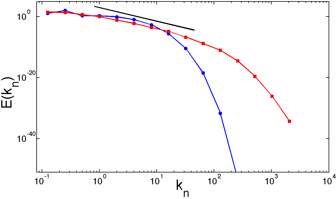
In order to understand whether the shell model defined via Eqs. (1) and (2) indeed shows the typical features of elastic turbulence, we perform numerical simulations of the shell model with and a stochastic forcing. The parameters (see Table 1) are such that for the shell model is not turbulent. The time-averaged (in the steady state) kinetic-energy spectrum indeed decreases sharply with the wavenumber without any apparent power-law scaling (see the blue line with filled circles in Fig. 1).
A typical signature for elastic turbulence is the development of a power-law energy spectrum with an exponent smaller than as the Weissenberg number is increased at fixed Reynolds number much smaller than 1 [6, 45]. We therefore turn on the polymer field in the shell model (), and for sufficiently large and a power-law scaling emerges. In Fig. 1, the energy spectrum for and is shown (red squares). We see a clear power-law behaviour, namely , as is indicated by the thick black line. The value of the exponent is close to that found in experiments [6, 45] and in numerical simulations [9, 10, 46, 47] and is consistent with the theoretical predictions based on the Oldroyd-B model [48]. The spectrum of the polymer end-to-end separation field does not show a power-law behaviour and is concentrated around small wave numbers, in agreement with direct numerical simulations of elastic turbulence [15]. An analogous behaviour is found with a deterministic forcing. This is accompanied by a corresponding increase of the largest Lyapunov exponent as discussed in detail later. The spectrum of the polymer end-to-end separation field does not show a power-law behaviour and is concentrated around small wave numbers, in agreement with direct numerical simulations of elastic turbulence [15]. Thus, the shell model reproduces the most obvious signature of elastic turbulence, namely, the emergence of a large-scale chaotic dynamics in a laminar flow with the addition of polymers.
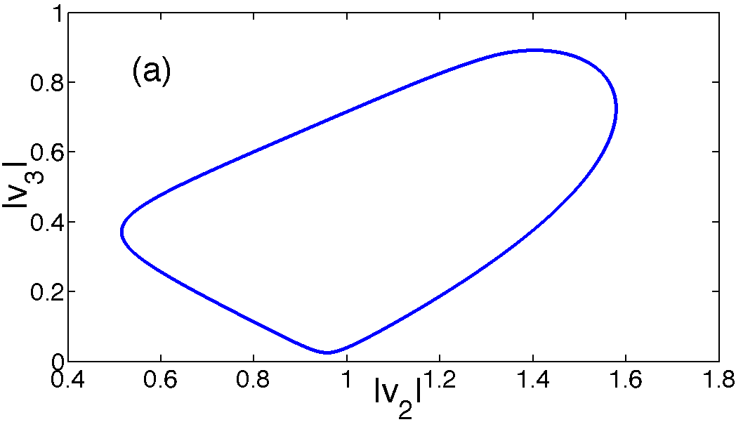
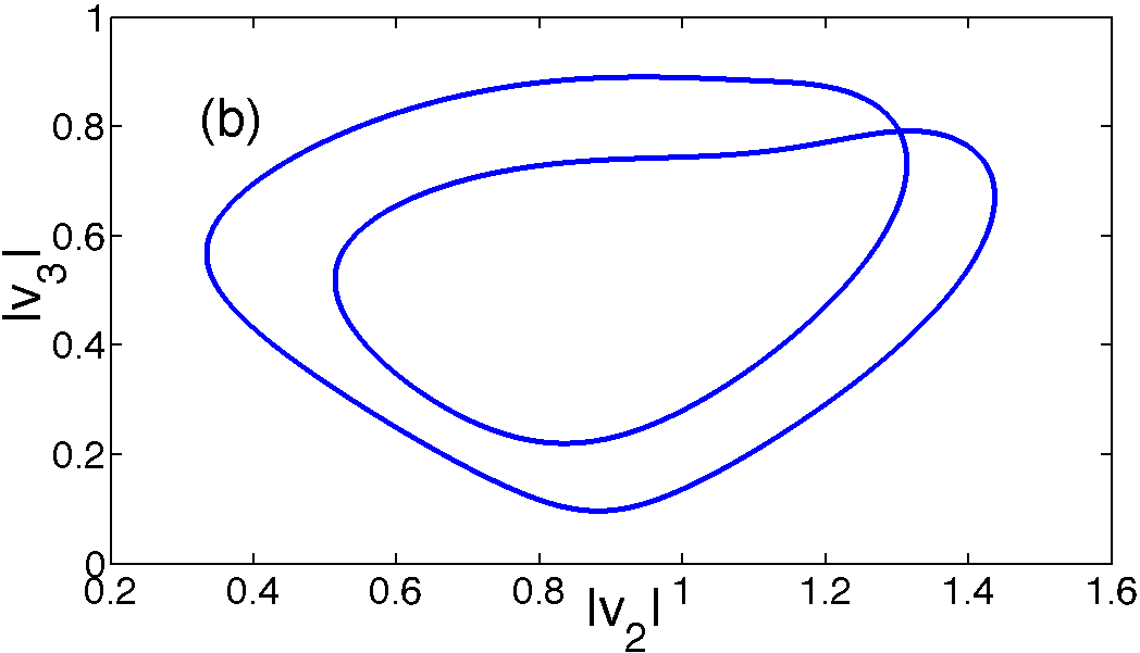
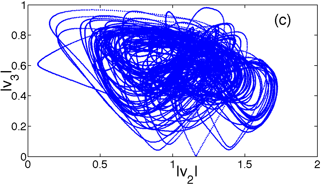
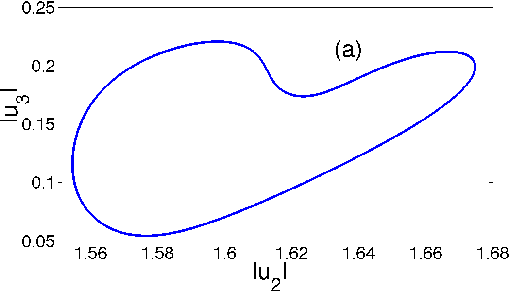
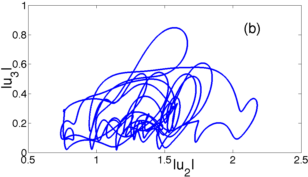
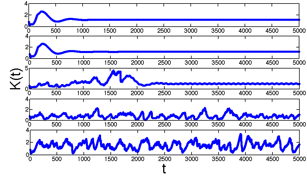
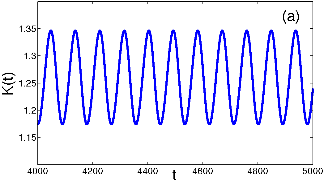
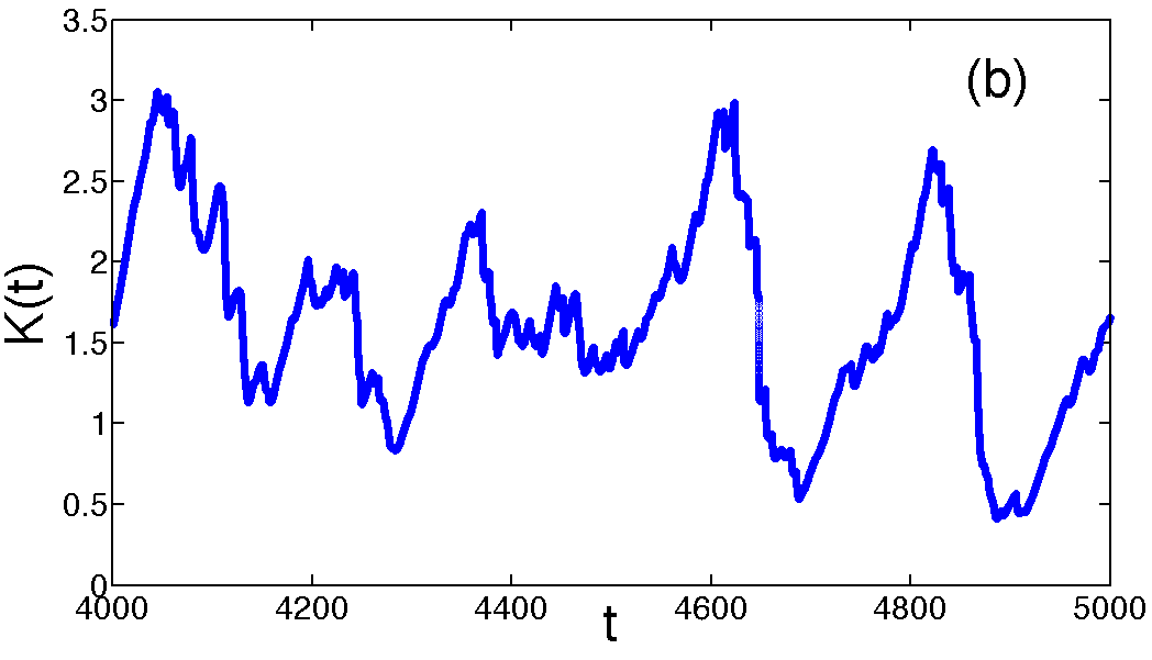
A global quantity like the total kinetic energy provides further insight into the transition to elastic turbulence; its temporal behaviour with varying Wi and indeed is an indicator of the changes of dynamical regime which happen in the system [10]. In Fig. 2 we show time series of for various combinations of and . For cases with very small values of —and independent of the value of —the total energy quickly saturates to an asymptotic value with no noticeable fluctuations, as is typical for laminar flows (Fig. 2, top two panels). However, as increases, even for a small enough value of , tiny but regular oscillations are seen in the temporal dynamics of vs (Fig. 2, middle panel). This behaviour is shown clearly in a zoomed plot in Fig. 3(a). Keeping the Weissenberg number fixed, we now increase the concentration (Fig. 2, bottom two panels) and see that the total kinetic energy vs time shows increasingly chaotic dynamics with large irregular fluctuations. This behaviour is highlighted in the zoomed-in Fig. 3(b). Figures 2 and 3 show that the shell model (which for is laminar because of our choice of parameters), with increasing effect of polymers characterised by the concentration or the Weissenberg number, undergoes a transition from a laminar phase to one with strong fluctuations through a series of intermediate periodic phases for moderate values of and . This phenomenon was first observed as a function of Wi in direct numerical simulations of the Oldroyd-B model [42] with periodic Kolmogorov forcing [10] and of the FENE-P model [42] in a cellular flow [15]. The shell model considered here not only reproduces such a transition to chaos through periodic states as the Weissenberg number is increased, but also shows that an analogous transition occurs as a function of polymer concentration. Following Ref. [44], in Fig. 4 we also show the map vs , for . The structure of this map for increasing values of further shows that the elastic-turbulence regime emerges through period doubling.
The above results confirm that the shell model with polymer additives replicates the global features of elastic turbulence. Given the relative numerical simplicity of shell models, it now behooves us to study in detail the effects of concentration on the small-scale mixing properties of elastic turbulence, which determine the importance of this phenomenon for practical applications. We quantify mixing in elastic turbulence and its dependence on and by calculating the largest Lyapunov exponent of the projection of the shell model on the variables. We recall that for the fluid GOY shell model such calculations show the chaotic–non-chaotic transitions as a function of the single parameter [43, 44]. For this set of calculations we would like to ensure that, in the absence of polymers, the flow is non-chaotic in order to reveal the transition to chaos more clearly. Thus we now study the shell model with (see Table 1), for which when . In order to check the generality of our conclusions, we use both a deterministic and a stochastic forcing and find our results insensitive to the precise nature of forcing.
Before we turn our attention to a quantitative measure of the transition to elastic turbulence below, we immediately note, as seen in Fig 5, that the basic feature of transition to chaos, with increasing concentration for a fixed , persists even for the case of .
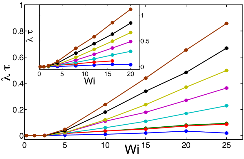
In Figure 6 we show the Lyapunov exponent rescaled with the polymer relaxation time, , as a function of for different values of both for deterministic and for stochastic forcing (inset). For small values of , the rescaled Lyapunov exponent remains close to 0, and hence the system is non-chaotic or laminar. For sufficiently large values of , we find that beyond a threshold value of the Weissenberg number () the rescaled Lyapunov exponent increases approximately linearly and for the largest value of , at , we find . Our findings are in agreement with analogous calculations made in the viscoleastic Kolmogorov flow for a single, fixed value of the elasticity of the flow [9]. It is important to note, though, that the results for the Kolmogorov flow [9] indicates a slightly more dramatic increase of as a function of the Weissenberg number than seen in the shell model.
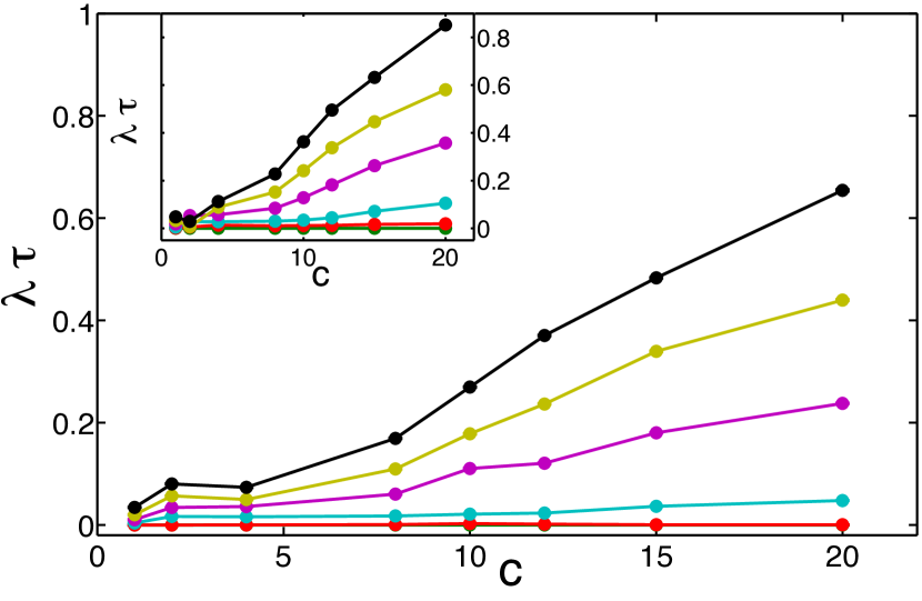
We now turn to the behaviour of as a function of for different values of , as shown in Fig. 7. As before we find that for low Weissenberg numbers, the flow remains non-chaotic even when the polymer concentration increases. Beyond a threshold value of , there is a sharp increase in when the concentration becomes greater than 5. Thus, provided Wi is sufficiently large, increasing the concentration has a destabilizing effect comparable to that observed when the Weissenberg number is increased.
Finally, the interaction between the polymers and the flow is described by the energy exchange [33]:
| (3) |
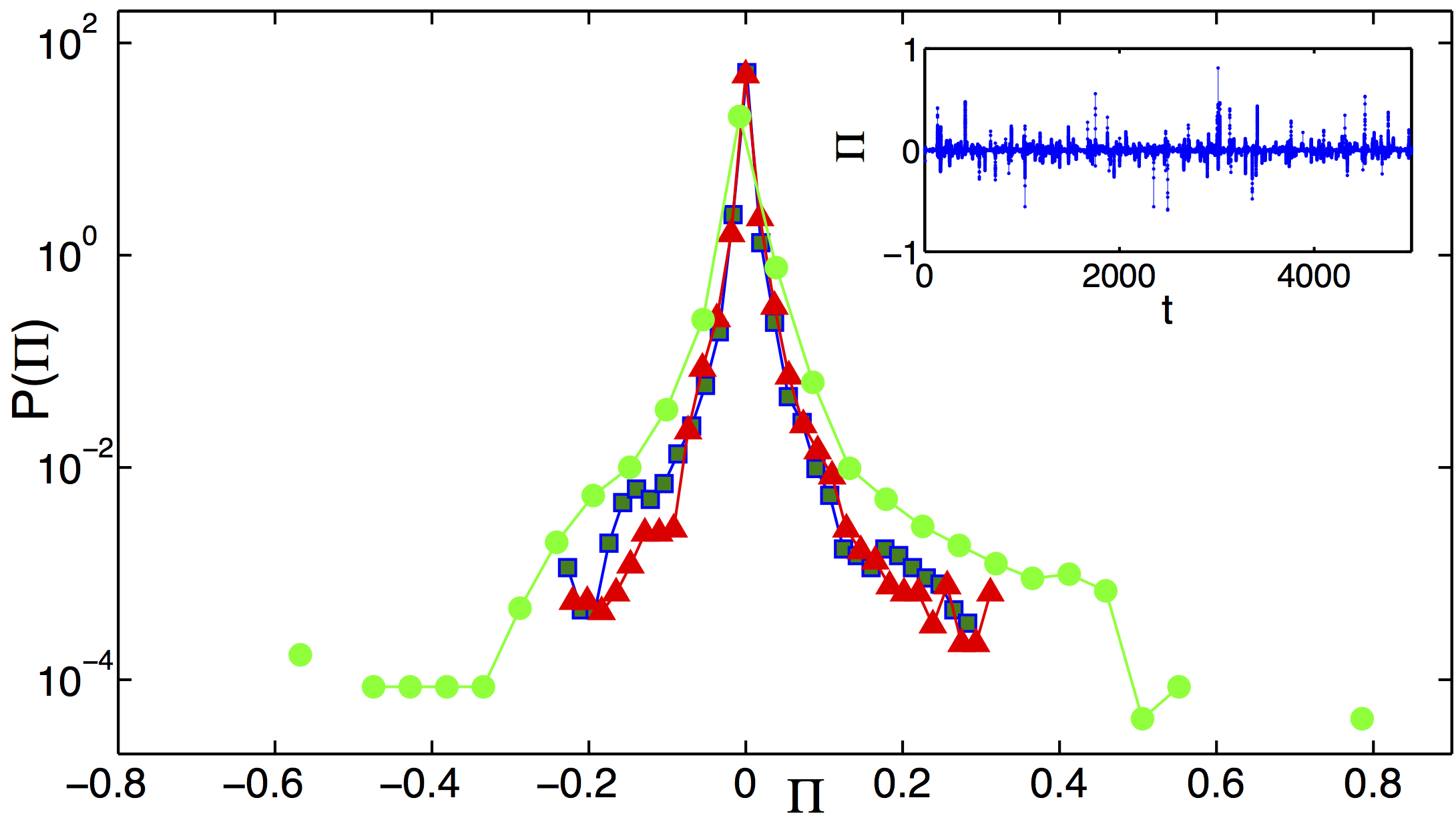
Negative values of indicate that energy flows from the velocity variables towards the polymers; positive values of correspond to energy transfers in the opposite direction. In turbulent drag reduction, the timeseries of is predominantly negative [28, 33]. This fact signals that polymers drain energy from the flow and justifies the description of their effect as a scale-dependent effective viscosity [33]. In Fig. 8, we show the probability density function of in the elastic-turbulence regime of the shell model with at different concentrations for a fixed value . We find that takes positive and negative values with comparable probabilities, i.e. in elastic turbulence there are continuous energy transfers between the flow and the polymers without a definite preferential direction (see also inset of Fig. 8. This result is consistent with the behaviour of the energy-exchange rate in decaying isotropic turbulence with polymer additives, the long-time stage of which has properties in common with elastic turbulence [47].
4 Conclusions
We have considered a shell model of viscoelastic fluid that describes the coupled dynamics of the velocity and polymer fields in the flow of a polymer solution. In the regime of large inertia and large elasticity, this model was previously shown to reproduce the main features of turbulent drag reduction. We have studied the regime in which inertial nonlinearities are negligible and have shown that, when the Weissenberg number becomes sufficiently high, the system shows a transition to a chaotic state. A detailed analysis of this chaotic state indicates that the shell model under consideration qualitatively reproduces the transition to elastic turbulence observed in experiments and in numerical simulations. The simplicity of the shell model also allows us to study the elastic-turbulence regime over a wide range of values not only of the Weissenberg number but also of polymer concentration. In particular, we find that, when the concentration is increased while the Weissenberg number is fixed, the emergence of the chaotic regime follows a dynamics analogous to that observed when the Weissenberg number is increased at fixed polymer concentration. Thus the transition to elastic turbulence shows similar features as a function of Wi and of .
This study enhances our understanding of the transition to elastic turbulence in polymer solutions. The shell model that we have studied mimicks the interactions between the Fourier modes of the velocity field and of the polymer end-to-end separation field in a viscoelastic fluid, but it contains no information on the spatial structure of these fields. The fact that such a model can replicate the main features of elastic turbulence shows that the specific geometrical configuration of the system does not play an essential role in the transition to elastic turbulence and that the physical mechanisms leading to elastic turbulence do not rely on the boundary conditions or on the mean flow.
5 Acknowledgments
The authors are grateful to Chirag Kalelkar and Stefano Musacchio for useful discussions. This work was supported in part by the Indo–French Centre for Applied Mathematics (IFCAM) and by the EU COST Action MP 1305 “Flowing Matter”. SSR acknowledges support from the AIRBUS Group Corporate Foundation in Mathematics of Complex Systems established at ICTS and the hospitality of the Observatoire de la Côte d’Azur, Nice, France. DV acknowledges the hospitality of ICTS-TIFR, Bangalore, India.
References
- [1] \NameGroisman A. Steinberg V. \REVIEWNature405200053.
- [2] \NameGroisman A. Steinberg V. \REVIEWNature4102001905.
- [3] \NameBurghelea T., Segre E., Bar-Joseph I., Groisman A. Steinberg V. \REVIEWPhys. Rev. E692004066305.
- [4] \NameLiu Y. Steinberg V. \REVIEWMacromol. Symp.337201434.
- [5] \NameMitchell J., Lyons K., Howe A. M. Clarke A. \REVIEWSoft Matter122016460.
- [6] \NameGroisman A. Steinberg V. \REVIEWNew J. Phys.6200429.
- [7] \NameBoffetta G., Celani A., Mazzino A., Puliafito A. Vergassola M. \REVIEWJ. Fluid Mech.5232005161.
- [8] \NameBistagnino A., Boffetta G., Celani A., Mazzino A., Puliafito A. Vergassola M. \REVIEWJ. Fluid Mech.590200761.
- [9] \NameBerti S., Bistagnino A., Boffetta G., Celani A. Musacchio S. \REVIEWPhys. Rev. E772008055306(R).
- [10] \NameBerti S. Boffetta G. \REVIEWPhys. Rev. E822010036314.
- [11] \NameMeulenbroek B., Storm C., Morozov A. N. van Saarloos W. \REVIEWJ. Non-Newtonian Fluid Mech.1162004235.
- [12] \NameMorozov A. N. van Saarloos W. \REVIEWPhys. Rev. Lett.952005024501.
- [13] \NamePan L., Morozov A., Wagner C Arratia P. E. \REVIEWPhys. Rev. Lett.1102013174502.
- [14] \NameBodiguel H., Beaumont J., Machado A., Martinie L., Kellay H. Colin A. \REVIEWPhys. Rev. Lett.1142015028302.
- [15] \NameGupta A. Pandit R. arXiv:1602.08153
- [16] \NameFrisch U. \BookTurbulence: The Legacy of Kolmogorov \PublCambridge University Press, Cambridge \Year1995.
- [17] \NameBohr T., Jensen M. H., Paladin G. Vulpiani A. \BookDynamical Systems Approach to Turbulence \PublCambridge University Press, Cambridge \Year1998.
- [18] \NameBiferale L. \REVIEWAnnu. Rev. Fluid Mech.352003441.
- [19] \NamePandit R., Perlekar P. Ray S. S. \REVIEWPramana - Journal of Physics732009157.
- [20] \NameJensen M. H., Paladin G. Vulpiani A. \REVIEWPhys. Rev. A4519927214
- [21] \NameWirth A. Biferale L. \REVIEWPhys. Rev. E5419964982.
- [22] \NameMitra D. Pandit R. \REVIEWPhys. Rev. Lett.952005144501.
- [23] \NameRay S. S., Mitra D. Pandit R. \REVIEWNew J. Phys.102008033003.
- [24] \NamePlunian F., Stepanov R. Frick P. \REVIEWPhys. Rep.52320131.
- [25] \NameChakraborty S., Jensen M. H. Sarker A. \REVIEWEur. Phys. J. B732010447.
- [26] \NameJensen M. H. Olesen P. \REVIEWPhysica D1111998243.
- [27] \NameRay S. S. Basu A. \REVIEWPhys. Rev. E842011036316.
- [28] \NameBenzi R., De Angelis E., Govindarajan R. Procaccia I. \REVIEWPhys. Rev. E682003016308.
- [29] \NameKalelkar C., Govindarajan R. Pandit R. \REVIEWPhys. Rev. E722005017301; \REVIEWibid.832011039903(E).
- [30] \NameConstantin P., Levant B. Titi E. S. \REVIEWPhysica D2192006120.
- [31] \NameFlandoli F. \BookRandom Perturbation of PDEs and Fluid Dynamic Models \PublSpringer–Verlag, Berlin \Year2011.
- [32] \NameBenzi R., Ching E. S. C., Horesh N. Procaccia I. \REVIEWPhys. Rev. Lett.922004078302.
- [33] \NameBenzi R., Ching E. S. C. Procaccia I. \REVIEWPhys. Rev. E702004026304.
- [34] \NameBenzi R., Horesh N. Procaccia I. \REVIEWEurophys. Lett.682004310.
- [35] \NameBenzi R., Ching E. S. C. De Angelis E. \REVIEWPhys. Rev. Lett.1042010024502.
- [36] \NameBenzi R, Ching E. S. C. Wong C. K. \REVIEWPhys. Rev. E892014053001.
- [37] \NameFrick P. Sokoloff D. \REVIEWPhys. Rev. E5719984155.
- [38] \NameChakraborty S., Jensen M. H. Sarker A. \REVIEWEur. Phys. J. B732010447.
- [39] \NameBasu A., Sain A., Dhar S. Pandit R. \REVIEWPhys. Rev. Lett.8119982687.
- [40] \NameGledzer E. \REVIEWSov. Phys. Dokl.181973216.
- [41] \NameYamada M. Ohkitani K. \REVIEWJ. Phys. Soc. Japan5619874210.
- [42] \NameBird R. B., Curtiss C. F., Armstrong R. C., Hassager O. \BookDynamics of Polymeric Fluids \Vol2 \PublWiley, New York \Year1987.
- [43] \NameBiferale L., Lambert A., Lima R. Paladin G. \REVIEWPhysica D801995105.
- [44] \NameKockelkoren J., Okkels F. Jensen M. H. \REVIEWJ. Stat. Phys.931998833.
- [45] \NameBurghelea T., Segre E. Steinberg V. \REVIEWPhys. Fluids192007053104.
- [46] \NameWatanabe T. Gotoh T. \REVIEWJ. Phys.: Conf. Ser.4542013012007.
- [47] \NameWatanabe T. Gotoh T. \REVIEWPhys. Fluids262014035110.
- [48] \NameFouxon A. Lebedev V. \REVIEWPhys. Fluids1520072060.