Network Morphism

Abstract

We present in this paper a systematic study on how to morph a well-trained neural network to a new one so that its network function can be completely preserved. We define this as network morphism in this research. After morphing a parent network, the child network is expected to inherit the knowledge from its parent network and also has the potential to continue growing into a more powerful one with much shortened training time. The first requirement for this network morphism is its ability to handle diverse morphing types of networks, including changes of depth, width, kernel size, and even subnet. To meet this requirement, we first introduce the network morphism equations, and then develop novel morphing algorithms for all these morphing types for both classic and convolutional neural networks. The second requirement for this network morphism is its ability to deal with non-linearity in a network. We propose a family of parametric-activation functions to facilitate the morphing of any continuous non-linear activation neurons. Experimental results on benchmark datasets and typical neural networks demonstrate the effectiveness of the proposed network morphism scheme.

1 Introduction

Figure 1: Illustration of network morphism. The child network is expected to inherit the entire knowledge from the parent network with the network function preserved. A variety of morphing types are illustrated. The change of segment $AC$ represents the depth morphing: $s\to s+t$; the inflated node $r$ involves width and kernel size morphing; a subnet is embedded in segment $CD$, which is subnet morphing. Complex network morphism can also be achieved with a combination of these basic morphing operations.

Deep convolutional neural networks (DCNNs) have achieved state-of-the-art results on diverse computer vision tasks such as image classification (Krizhevsky et al., 2012; Simonyan & Zisserman, 2014; Szegedy et al., 2014), object detection (Girshick et al., 2014; Girshick, 2015; Ren et al., 2015), and semantic segmentation (Long et al., 2014). However, training such a network is very time-consuming. It usually takes weeks or even months to train an effective deep network, let alone the exploration of diverse network settings. It is very much desired for these well-trained networks to be directly adopted for other related applications with minimum retraining.

To accomplish such an ideal goal, we need to systematically study how to morph a well-trained neural network to a new one with its network function completely preserved. We call such operations network morphism. Upon completion of such morphism, the child network shall not only inherit the entire knowledge from the parent network, but also be capable of growing into a more powerful one in much shortened training time as the process continues on. This is fundamentally different from existing work related to network knowledge transferring, which either tries to mimic a parent network’s outputs (Bucilu et al., 2006; Ba & Caruana, 2014; Romero et al., 2014), or pre-trains to facilitate the convergence and/or adapt to new datasets with possible total change in network function (Simonyan & Zisserman, 2014; Oquab et al., 2014).

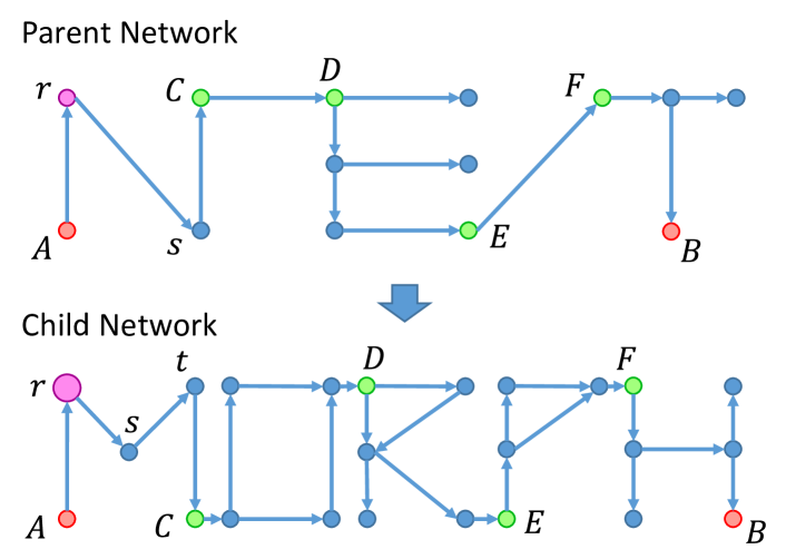
Mathematically, a morphism is a structure-preserving map from one mathematical structure to another (Weisstein, 2002). In the context of neural networks, network morphism refers to a parameter-transferring map from a parent network to a child network that preserves its function and outputs. Although network morphism generally does not impose constraints on the architecture of the child network, we limit the investigation of network morphism to the expanding mode, which intuitively means that the child network is deeper and/or wider than its parent network. Fig. 1 illustrates the concept of network morphism, where a variety of morphing types are demonstrated including depth morphing, width morphing, kernel size morphing, and subnet morphing. In this work, we derive network morphism equations for a successful morphing operation to follow, based on which novel network morphism algorithms can be developed for all these morphing types. The proposed algorithms work for both classic multi-layer perceptron models and convolutional neural networks. Since in the proposed network morphism it is required that the output is unchanged, a complex morphing can be decomposed into basic morphing steps, and thus can be solved easily.

Depth morphing is an important morphing type, since current top-notch neural networks are going deeper and deeper (Krizhevsky et al., 2012; Simonyan & Zisserman, 2014; Szegedy et al., 2014; He et al., 2015a). One heuristic approach is to embed an identity mapping layer into the parent network, which is referred as IdMorph. IdMorph is explored by a recent work (Chen et al., 2015), but is potentially problematic due to the sparsity of the identity layer, and might fail sometimes (He et al., 2015a). To overcome the issues associated with IdMorph, we introduce several practices for the morphism operation to follow, and propose a deconvolution-based algorithm for network depth morphing. This algorithm is able to asymptotically fill in all parameters with non-zero elements. In its worst case, the non-zero occupying rate of the proposed algorithm is still higher than IdMorph for an order of magnitude.

Another challenge the proposed network morphism will face is the dealing of the non-linearity in a neural network. Even the simple IdMorph method fails in this case, because it only works for idempotent functions. In this work, to deal with the non-linearity, we introduce the concept of parametric-activation function family, which is defined as an adjoint function family for arbitrary non-linear activation function. It can reduce the non-linear operation to a linear one with a parameter that can be learned. Therefore, the network morphism of any continuous non-linear activation neurons can be solved.

To the best of our knowledge, this is the first work about network morphism, except the recent work (Chen et al., 2015) that introduces the IdMorph. We conduct extensive experiments to show the effectiveness of the proposed network morphism learning scheme on widely used benchmark datasets for both classic and convolutional neural networks. The effectiveness of basic morphing operations are also verified. Furthermore, we show that the proposed network morphism is able to internally regularize the network, that typically leads to an improved performance. Finally, we also successfully morph the well-known 16-layered VGG net (Simonyan & Zisserman, 2014) to a better performing model, with only ${\textstyle\frac{1}{15}}$ of the training time comparing against the training from scratch.

2 Related Work

We briefly introduce recent work related to network morphism and identify the differences from this work.

Mimic Learning. A series of work trying to mimic the teacher network with a student network have been developed, which usually need learning from scratch. For example, (Bucilu et al., 2006) tried to train a lighter network by mimicking an ensemble network. (Ba & Caruana, 2014) extended this idea, and used a shallower but wider network to mimic a deep and wide network. In (Romero et al., 2014), the authors adopted a deeper but narrower network to mimic a deep and wide network. The proposed network morphism scheme is different from these algorithms, since instead of mimicking, its goal is to make the child network directly inherit the intact knowledge (network function) from the parent network. This allows network morphism to achieve the same performance. That is why the networks are called parent and child, instead of teacher and student. Another major difference is that the child network is not learned from scratch.

Pre-training and Transfer Learning. Pre-training (Simonyan & Zisserman, 2014) is a strategy proposed to facilitate the convergence of very deep neural networks, and transfer learning (Simonyan & Zisserman, 2014; Oquab et al., 2014) is introduced to overcome the overfitting problem when training large neural networks on relatively small datasets. They both re-initialize the last few layers of the parent network with the other layers remaining the same (or refined in a lighter way). Their difference is that pre-training continues to train the child network on the same dataset, while transfer learning continues on a new one. However, these two strategies totally alter the parameters in the last few layers, as well as the network function.

Net2Net. Net2Net is a recent work proposed in (Chen et al., 2015). Although it targets at the same problem, there are several major differences between network morphism and Net2Net. First, the solution of Net2Net is still restricted to the IdMorph approach, while NetMorph is the first to make it possible to embed non-identity layers. Second, Net2Net’s operations only work for idempotent activation functions, while NetMorph is the first to handle arbitrary non-linear activation functions. Third, Net2Net’s discussion is limited to width and depth changes, while NetMorph studies a variety of morphing types, including depth, width, kernel size, and subnet changes. Fourth, Net2Net needs to separately consider depth and width changes, while NetMorph is able to simultaneously conduct depth, width, and kernel size morphing in a single operation.

3 Network Morphism

We shall first discuss the depth morphing in the linear case, which actually also involves with width and kernel size morphing. Then we shall describe how to deal with the non-linearities in the neural networks. Finally, we shall present the stand-alone versions for width morphing and kernel size morphing, followed by the subnet morphing.

3.1 Network Morphism: Linear Case

Let us start from the simplest case of a classic neural network. We first drop all the non-linear activation functions and consider a neural network only connected with fully connected layers.

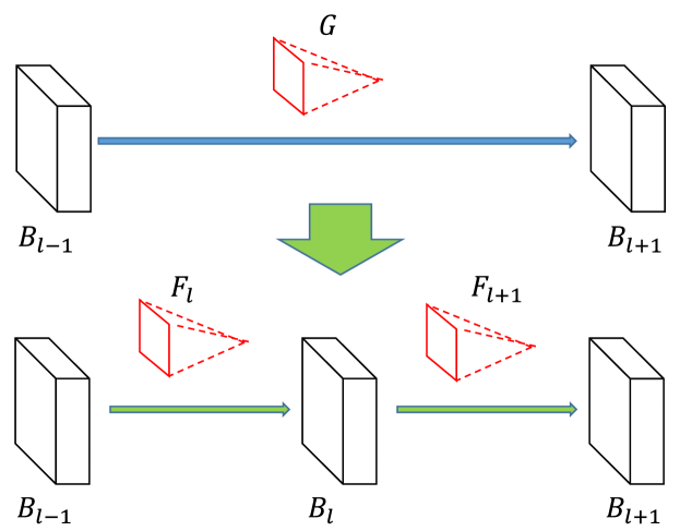
As shown in Fig. 2, in the parent network, two hidden layers $B_{l-1}$ and $B_{l+1}$ are connected via the weight matrix $G$:

$$B_{l+1}=G\cdot B_{l-1},$$ (1)

where $B_{l-1}\in\mathbb{R}^{C_{l-1}}$, $B_{l+1}\in\mathbb{R}^{C_{l+1}}$, $G\in\mathbb{R}^{C_{l+1}\times C_{l-1}}$, $C_{l-1}$ and $C_{l+1}$ are the feature dimensions of $B_{l-1}$ and $B_{l+1}$. For network morphism, we shall insert a new hidden layer $B_{l}$, so that the child network satisfies:

$$B_{l+1}=F_{l+1}\cdot B_{l}=F_{l+1}\cdot(F_{l}\cdot B_{l-1})=G\cdot B_{l-1},$$ (2)

where $B_{l}\in\mathbb{R}^{C_{l}}$, $F_{l}\in\mathbb{R}^{C_{l}\times C_{l-1}}$, and $F_{l+1}\in\mathbb{R}^{C_{l+1}\times C_{l}}$. It is obvious that network morphism for classic neural networks is equivalent to a matrix decomposition problem:

$$G=F_{l+1}\cdot F_{l}.$$ (3)

Next, we consider the case of a deep convolutional neural network (DCNN). For a DCNN, the build-up blocks are convolutional layers rather than fully connected layers. Thus, we call the hidden layers as blobs, and weight matrices as filters. For a 2D DCNN, the blob $B_{*}$ is a 3D tensor of shape $(C_{*},H_{*},W_{*})$, where $C_{*}$, $H_{*}$, and $W_{*}$ represent the number of channels, height and width of $B_{*}$. The filters $G$, $F_{l}$, and $F_{l+1}$ are 4D tensors of shapes $(C_{l+1},C_{l-1},K,K)$, $(C_{l},C_{l-1},K_{1},K_{1})$, and $(C_{l+1},C_{l},K_{2},K_{2})$, where $K$, $K_{1}$, $K_{2}$ are convolutional kernel sizes.

The convolutional operation in a DCNN can be defined in a multi-channel way:

$$B_{l}(c_{l})=\sum_{c_{l-1}}B_{l-1}(c_{l-1})*F_{l}(c_{l},c_{l-1}),$$ (4)

where $*$ is the convolution operation defined in a traditional way. It is easy to derive that the filters $F_{l},$ $F_{l+1}$ and $G$ shall satisfy the following equation:

$$\tilde{G}(c_{l+1},c_{l-1})=\sum_{c_{l}}F_{l}(c_{l},c_{l-1})*F_{l+1}(c_{l+1},c_{l}),$$ (5)

where $\tilde{G}$ is a zero-padded version of $G$ whose effective kernel size (receptive field) is $\tilde{K}=K_{1}+K_{2}-1\geq K$. If $\tilde{K}=K$, we will have $\tilde{G}=G$.

Figure 2: Network morphism linear. $B_{*}$ represents blobs (hidden units), $G$ and $F_{*}$ are convolutional filters (weight matrices) for DCNNs (classic neural networks). $G$ is morphed into $F_{l}$ and $F_{l+1}$, satisfying the network morphism equation (6).

Mathematically, inner products are equivalent to multi-channel convolutions with kernel sizes of $1\times 1$. Thus, Equation (3) is equivalent to Equation (5) with $K=K_{1}=K_{2}=1$. Hence, we are able to unify them into one equation:

$$\tilde{G}=F_{l+1}\circledast F_{l},$$ (6)

where $\circledast$ is a non-communicative operator that can either be an inner product or a multi-channel convolution. We call Equation (6) as the network morphism equation (for depth in the linear case).

Although Equation (6) is primarily derived for depth morphing ($G$ morphs into $F_{l}$ and $F_{l+1}$), it also involves network width $($the choice of $C_{l}$), and kernel sizes (the choice of $K_{1}$ and $K_{2}$). Thus, it will be called network morphism equation for short for the remaining of this paper.

The problem of network depth morphing is formally formulated as follows:

Input:

$G$ of shape $(C_{l+1},C_{l-1},K,K)$; $C_{l}$, $K_{1}$, $K_{2}$.

Output:

$F_{l}$ of shape $(C_{l},C_{l-1},K_{1},K_{1})$, $F_{l+1}$ of shape $(C_{l+1},C_{l},K_{2},K_{2})$ that satisfies Equation (6).

3.2 Network Morphism Algorithms: Linear Case

In this section, we introduce two algorithms to solve for the network morphism equation (6).

Since the solutions to Equation (6) might not be unique, we shall make the morphism operation to follow the desired practices that: 1) the parameters will contain as many non-zero elements as possible, and 2) the parameters will need to be in a consistent scale. These two practices are widely adopted in existing work, since random initialization instead of zero filling for non-convex optimization problems is preferred (Bishop, 2006), and the scale of the initializations is critical for the convergence and good performance of deep neural networks (Glorot & Bengio, 2010; He et al., 2015b).

Next, we introduce two algorithms based on deconvolution to solve the network morphism equation (6), i.e., 1) general network morphism, and 2) practical network morphism. The former one fills in all the parameters with non-zero elements under certain condition, while the latter one does not depend on such a condition but can only asymptotically fill in all parameters with non-zero elements.

3.2.1 General Network Morphism

This algorithm is proposed to solve Equation (6) under certain condition. As shown in Algorithm 1, it initializes convolution kernels $F_{l}$ and $F_{l+1}$ of the child network with random noises. Then we iteratively solve $F_{l+1}$ and $F_{l}$ by fixing the other. For each iteration, $F_{l}$ or $F_{l+1}$ is solved by deconvolution. Hence the overall loss is always decreasing and is expected to converge. However, it is not guaranteed that the loss in Algorithm 1 will always converge to 0.

We claim that if the parameter number of either $F_{l}$ or $F_{l+1}$ is no less than $\tilde{G}$, Algorithm 1 shall converge to 0.

Claim 1.

If the following condition is satisfied, the loss in Algorithm 1 shall converge to 0 (in one step):

$$\min(C_{l}C_{l-1}K_{1}^{2},C_{l+1}C_{l}K_{2}^{2})\geq C_{l+1}C_{l-1}(K_{1}+K_{2}-1)^{2}.$$ (7)

The three items in condition (7) are the parameter numbers of $F_{l}$ ,$F_{l+1}$, and $\tilde{G}$, respectively.

It is easy to check the correctness of Condition (7), as a multi-channel convolution can be written as the multiplication of two matrices. Condition (7) claims that we have more unknowns than constraints, and hence it is an undetermined linear system. Since random matrices are rarely inconsistent (with probability 0), the solutions of the undetermined linear system always exist.

3.2.2 Practical Network Morphism

Algorithm 1 General Network Morphism

  Input: $G$ of shape $(C_{l+1},C_{l-1},K,K)$; $C_{l}$, $K_{1}$, $K_{2}$

  Output: $F_{l}$ of shape $(C_{l},C_{l-1},K_{1},K_{1})$, $F_{l+1}$ of shape $(C_{l+1},C_{l},K_{2},K_{2})$

  Initialize $F_{l}$ and $F_{l+1}$ with random noise.

  Expand $G$ to $\tilde{G}$ with kernel size $\tilde{K}=K_{1}+K_{2}-1$ by padding zeros.

  repeat

     Fix $F_{l}$, and calculate $F_{l+1}=deconv(\tilde{G},F_{l})$

     Fix $F_{l+1}$, and calculate $F_{l}=deconv(\tilde{G},F_{l+1})$

     Calculate loss $l=\|\tilde{G}-conv(F_{l},F_{l+1})\|^{2}$

  until $l=0$ or $maxIter$ is reached

  Normalize $F_{l}$ and $F_{l+1}$ with equal standard variance.

Algorithm 2 Practical Network Morphism

  Input: $G$ of shape $(C_{l+1},C_{l-1},K,K)$; $C_{l}$, $K_{1}$, $K_{2}$

  Output: $F_{l}$ of shape $(C_{l},C_{l-1},K_{1},K_{1})$, $F_{l+1}$ of shape $(C_{l+1},C_{l},K_{2},K_{2})$

  /* For simplicity, we illustrate this algorithm for the case ‘$F_{l}$ expands $G$’ */

  $K_{2}^{r}=K_{2}$

  repeat

     Run Algorithm 1 with $maxIter$ set to 1: $l,F_{l},F_{l+1}^{r}=\textsc{NetMorphGeneral}(G;C_{l},K_{1},K_{2}^{r})$

     $K_{2}^{r}=K_{2}^{r}-1$

  until $l=0$

  Expand $F_{l+1}^{r}$ to $F_{l+1}$ with kernel size $K_{2}$ by padding zeros.

  Normalize $F_{l}$ and $F_{l+1}$ with equal standard variance.

Next, we propose a variant of Algorithm 1 that can solve Equation (6) with a sacrifice in the non-sparse practice. This algorithm reduces the zero-converging condition to that the parameter number of either $F_{l}$ or $F_{l+1}$ is no less than $G$, instead of $\tilde{G}$. Since we focus on network morphism in an expanding mode, we can assume that this condition is self-justified, namely, either $F_{l}$ expands $G$, or $F_{l+1}$ expands $G$. Thus, we can claim that this algorithm solves the network morphism equation (6). As described in Algorithm 2, for the case that $F_{l}$ expands $G$, starting from $K_{2}^{r}=K_{2}$, we iteratively call Algorithm 1 and shrink the size of $K_{2}^{r}$ until the loss converges to 0. This iteration shall terminate as we are able to guarantee that if $K_{2}^{r}=1$, the loss is 0. For the other case that $F_{l+1}$ expands $G$, the algorithm is similar.

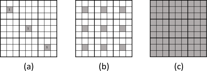
The sacrifice of the non-sparse practice in Algorithm 2 is illustrated in Fig. 3. In its worst case, it might not be able to fill in all parameters with non-zero elements, but still fill asymptotically. This figure compares the non-zero element occupations for IdMorph and NetMorph. We assume $C_{l+1}=O(C_{l})\triangleq O(C)$. In the best case (c), NetMorph is able to occupy all the elements by non-zeros, with an order of $O(C^{2}K^{2})$. And in the worst case (b), it has an order of $O(C^{2})$ non-zero elements. Generally, NetMorph lies in between the best case and worst case. IdMorph (a) only has an order of $O(C)$ non-zeros elements. Thus the non-zero occupying rate of NetMorph is higher than IdMorph for at least one order of magnitude. In practice, we shall also have $C\gg K$, and thus NetMorph can asymptotically fill in all parameters with non-zero elements.

3.3 Network Morphism: Non-linear Case

In the proposed network morphism it is also required to deal with the non-linearities in a neural network. In general, it is not trivial to replace the layer $B_{l+1}=\varphi(G\circledast B_{l+1})$ with two layers $B_{l+1}=\varphi(F_{l+1}\circledast\varphi(F_{l}\circledast B_{l-1}))$, where $\varphi$ represents the non-linear activation function.

For an idempotent activation function satisfying $\varphi\circ\varphi=\varphi,$ the IdMorph scheme in Net2Net (Chen et al., 2015) is to set $F_{l+1}=I$, and $F_{l}=G$, where $I$ represents the identity mapping. Then we have

$$\varphi(I\circledast\varphi(G\circledast B_{l-1})=\varphi\circ\varphi(G\circledast B_{l+1})=\varphi(G\circledast B_{l+1}).$$ (8)

However, although IdMorph works for the ReLU activation function, it cannot be applied to other commonly used activation functions, such as Sigmoid and TanH, since the idempotent condition is not satisfied.

To handle arbitrary continuous non-linear activation functions, we propose to define the concept of P(arametric)-activation function family. A family of P-activation functions for an activation function $\varphi$, can be defined to be any continuous function family that maps $\varphi$ to the linear identity transform $\varphi_{id}:x\mapsto x$. The P-activation function family for $\varphi$ might not be uniquely defined. We define the canonical form for P-activation function family as follows:

$$P\textit{-}\varphi\triangleq\{\varphi^{a}\}|_{a\in[0,1]}=\{(1-a)\cdot\varphi+a\cdot\varphi_{id}\}|_{a\in[0,1]},$$ (9)

where $a$ is the parameter to control the shape morphing of the activation function. We have $\varphi^{0}=\varphi$, and $\varphi^{1}=\varphi_{id}$. The concept of P-activation function family extends PReLU (He et al., 2015b), and the definition of PReLU coincides with the canonical form of P-activation function family for the ReLU non-linear activation unit.

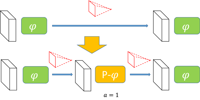
The idea of leveraging P-activation function family for network morphism is shown in Fig. 4. As shown, it is safe to add the non-linear activations indicated by the green boxes, but we need to make sure that the yellow box is equivalent to a linear activation initially. This linear activation shall grow into a non-linear one once the value of $a$ has been learned. Formally, we need to replace the layer $B_{l+1}=\varphi(G\circledast B_{l+1})$ with two layers $B_{l+1}=\varphi(F_{l+1}\circledast\varphi^{a}(F_{l}\circledast B_{l-1}))$. If we set $a=1$, the morphing shall be successful as long as the network morphing equation (6) is satisfied:

$$\varphi(F_{l+1}\circledast\varphi^{a}(F_{l}\circledast B_{l-1})) =\varphi(F_{l+1}\circledast F_{l}\circledast B_{l-1})$$ (10)

$$=\varphi(G\circledast B_{l-1}).$$ (11)

The value of $a$ shall be learned when we continue to train the model.

Figure 3: Non-zero element (indicated as gray) occupations of different algorithms: (a) IdMorph in $O(C)$, (b) NetMorph worst case in $O(C^{2})$, and (c) NetMorph best case in $O(C^{2}K^{2})$. $C$ and $K$ represent the channel size and kernel size. This figure shows a 4D convolutional filter of shape $(3,3,3,3)$ flattened in 2D. It can be seen that the filter in IdMorph is very sparse.

Figure 4: Network morphism non-linear. Activations indicated as green can be safely added; the activation in yellow needs to be set as linear ($a=1$) at the beginning, and then is able to grow into a non-linear one as $a$ is being learned.

3.4 Stand-alone Width and Kernel Size Morphing

As mentioned, the network morphism equation (6) involves network depth, width, and kernel size morphing. Therefore, we can conduct width and kernel size morphing by introducing an extra depth morphing via Algorithm 2.

Sometimes, we need to pay attention to stand-alone network width and kernel size morphing operations. In this section, we introduce solutions for these situations.

3.4.1 Width Morphing

For width morphing, we assume $B_{l-1},\ B_{l},\ B_{l+1}$ are all parent network layers, and the target is to expand the width (channel size) of $B_{l}$ from $C_{l}$ to $\tilde{C_{l}}$, $\tilde{C_{l}}\geq C_{l}$. For the parent network, we have

$$B_{l}(c_{l})=\sum_{c_{l-1}}B_{l-1}(c_{l-1})*F_{l}(c_{l},c_{l-1}),$$ (12)

$$B_{l+1}(c_{l+1})=\sum_{c_{l}}B_{l}(c_{l})*F_{l+1}(c_{l+1},c_{l}).$$ (13)

For the child network, $B_{l+1}$ should be kept unchanged:

$$B_{l+1}(c_{l+1})=\sum_{\tilde{c_{l}}}B_{l}(\tilde{c_{l}})*\tilde{F}_{l+1}(c_{l+1},\tilde{c_{l}})$$ (14)

$$=\sum_{c_{l}}B_{l}(c_{l})*F_{l+1}(c_{l+1},c_{l})+\sum_{\bar{c_{l}}}B_{l}(\bar{c_{l}})*\tilde{F}_{l+1}(c_{l+1},\bar{c_{l}}),$$ (15)

where $\tilde{c_{l}}$ and $c_{l}$ are the indices of the channels of the child network blob $\tilde{B_{l}}$ and parent network blob $B_{l}$. $\bar{c_{l}}$ is the index of the complement $\tilde{c_{l}}\backslash c_{l}$. Thus, we only need to satisfy:

$$0 =\sum_{\bar{c_{l}}}B_{l}(\bar{c_{l}})*\tilde{F}_{l+1}(c_{l+1},\bar{c_{l}})$$ (16)

$$=\sum_{\bar{c_{l}}}B_{l-1}(c_{l-1})*\tilde{F_{l}}(\bar{c_{l}},c_{l-1})*\tilde{F}_{l+1}(c_{l+1},\bar{c_{l}}),$$ (17)

or simply,

$$\tilde{F_{l}}(\bar{c_{l}},c_{l-1})*\tilde{F}_{l+1}(c_{l+1},\bar{c_{l}})=0.$$ (18)

It is obvious that we can either set $\tilde{F_{l}}(\bar{c_{l}},c_{l-1})$ or $\tilde{F}_{l+1}(c_{l+1},\bar{c_{l}})$ to 0, and the other can be set arbitrarily. Following the non-sparse practice, we set the one with less parameters to 0, and the other one to random noises. The zeros and random noises in $\tilde{F_{l}}$ and $\tilde{F}_{l+1}$ may be clustered together. To break this unwanted behavior, we perform a random permutation on $\tilde{c_{l}}$, which will not change $B_{l+1}$.

3.4.2 Kernel Size Morphing

Figure 5: Network morphism in kernel size. Both the filters and blobs are padded with the same size of zeros around to keep the final results unchanged.

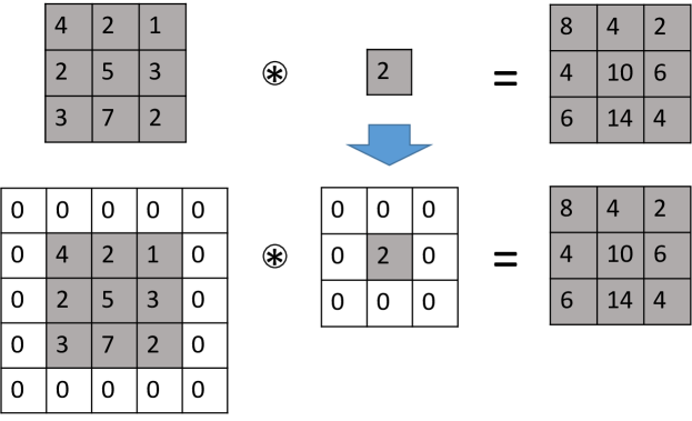
For kernel size morphing, we propose a heuristic yet effective solution. Suppose that a convolutional layer $l$ has kernel size of $K_{l}$, and we want to expand it to $\tilde{K_{l}}$. When the filters of layer $l$ are padded with $(\tilde{K_{l}}-K_{l})/2$ zeros on each side, the same operation shall also apply for the blobs. As shown in Fig. 5, the resulting blobs are of the same shape and also with the same values.

3.5 Subnet Morphing

(a) Typical subnets

(b) Sequential subnet morphing

(c) Stacked sequential subnet morphing

Figure 6: Subnet morphing. (a) Subnet examples of the mlpconv layer in NiN and inception layer in GoogleNet. (b) Sequential subnet morphing from a single layer to $P+1$ layers. (c) Workflow for stacked sequential subnet morphing.

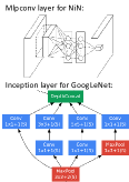
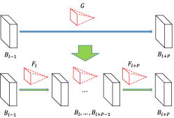
Modern networks are going deeper and deeper. It is challenging to manually design tens of or even hundreds of layers. One elegant strategy is to first design a subnet template, and then construct the network by these subnets. Two typical examples are the mlpconv layer for Network in Network (NiN) (Lin et al., 2013) and the inception layer for GoogLeNet (Szegedy et al., 2014), as shown in Fig. 6(a).

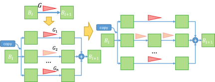
We study the problem of subnet morphing in this section, that is, network morphism from a minimal number (typically one) of layers in the parent network to a subnet in the child network. One commonly used subnet is the stacked sequential subnet as shown in Fig. 6(c). An exmaple is the inception layer for GoogLeNet with a four-way stacking of sequential subnets.

We first describe the morphing operation for the sequential subnet, based on which its stacked version is then obtained.

Sequential subnet morphing is to morph from a single layer to multiple sequential layers, as illustrated in Fig. 6(b). Similar to Equation (6), one can derive the network morphism equation for sequential subnets from a single layer to $P+1$ layers:

$$\tilde{G}(c_{l+P},c_{l-1})=\sum_{\mathclap{c_{l},\cdots,c_{l+P-1}}}F_{l}(c_{l},c_{l-1})*\cdots*F_{l+P}(c_{l+P},c_{l+P-1}),$$ (19)

where $\tilde{G}$ is a zero-padded version of $G$. Its effective kernel size is $\tilde{K}=\sum_{p=0,\cdots,P}K_{l+p}-P$, and $K_{l}$ is the kernel size of layer $l$. Similar to Algorithm 1, subnet morphing equation (19) can be solved by iteratively optimizing the parameters for one layer with the parameters for the other layers fixed. We can also develop a practical version of the algorithm that can solve for Equation (19), which is similar to Algorithm 2. The algorithm details are omitted here.

For stacked sequential subnet morphing, we can follow the work flow illustrated as Fig. 6(c). First, a single layer in the parent network is split into multiple paths. The split $\{G_{i}\}$ is set to satisfy

$${\displaystyle\sum_{i=1}^{n}G_{i}=G},$$ (20)

in which the simplest case is $G_{i}={\textstyle\frac{1}{n}}G$. Then, for each path, a sequential subnet morphing can be conducted. In Fig. 6(c), we illustrate an $n$-way stacked sequential subnet morphing, with the second path morphed into two layers.

4 Experimental Results

In this section, we conduct experiments on three datasets (MNIST, CIFAR10, and ImageNet) to show the effectiveness of the proposed network morphism scheme, on 1) different morphing operations, 2) both the classic and convolutional neural networks, and 3) both the idempotent activations (ReLU) and non-idempotent activations (TanH).

4.1 Network Morphism for Classic Neural Networks

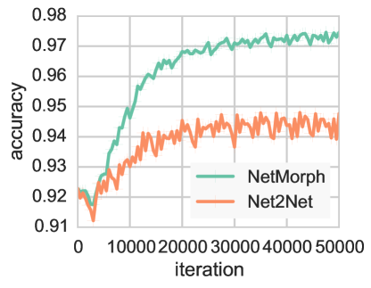
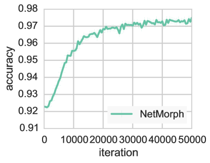
The first experiment is conducted on the MNIST dataset (LeCun et al., 1998). MNIST is a standard dataset for handwritten digit recognition, with 60,000 training images and 10,000 testing images. In this section, instead of using state-of-the-art DCNN solutions (LeCun et al., 1998; Chang & Chen, 2015), we adopt the simple softmax regression model as the parent network to evaluate the effectiveness of network morphism on classic networks. The gray-scale $28\times 28$ digit images were flattened as a $784$ dimension feature vector as input. The parent model achieved 92.29% accuracy, which is considered as the baseline. Then, we morphed this model into a multiple layer perception (MLP) model by adding a PReLU or PTanH hidden layer with the number of hidden neurons $h=50$. Fig. 7(a) shows the performance curves of NetMorph and Net2Net after morphing. We can see that, for the PReLU activation, NetMorph works much better than Net2Net. NetMorph continues to improve the performance from 92% to 97%, while Net2Net improves only to 94%. We also show the curve of NetMorph with the non-idempotent activation PTanH in Fig. 7(b). The curve for Net2Net is unavailable since it cannot handle non-idempotent activations.

(a) PReLU

(b) PTanH

Figure 7: Morphing on MNIST from softmax regression to multiple layer perception.

4.2 Depth Morphing, Subnet Morphing, and Internal Regularization for DCNN

(a) cifar_111 $\to$ 211

(b) cifar_211 $\to$ 222

(c) cifar_222 $\to$ 2222

(d) cifar_2222 $\to$ 3333

Figure 8: Depth morphing and subnet morphing on CIFAR10.

Extensive experiments were conducted on the CIFAR10 dataset (Krizhevsky & Hinton, 2009) to verify the network morphism scheme for convolutional neural networks. CIFAR10 is an image recognition database composed of $32\times 32$ color images. It contains 50,000 training images and 10,000 testing images for ten object categories. The baseline network we adopted is the Caffe (Jia et al., 2014) cifar10_quick model with an accuracy of 78.15%.

In the following, we use the unified notation cifar_ddd to represent a network architecture of three subnets, in which each digit d is the number of convolutional layers in the corresponding subnet. The detailed architecture of each subnet is described by (<kernel_size>:<num_output>,...). Following this notation, the cifar10_quick model, which has three convolutional layers and two fully connected layers, can be denoted as cifar_111, with its architecture described with (5:32)(5:32)(5:64). Additionally, we also use [<subnet>] to indicate the grouping of layers in a subnet, and x<times> to represent for the repetition of layers or subnets. Hence, cifar10_quick can also be denoted as (5:32)x2(5:64) or [(5:32)]x2[(5:64)]. Note that in this notation, the fully connected layers are ignored.

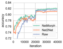
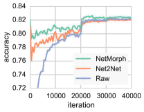
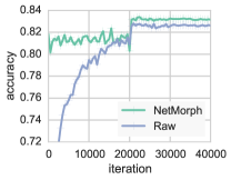
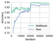
Fig. 8 shows the comparison results between NetMorph and Net2Net, in the morphing sequence of cifar_111$\to$211$\to$222$\to$2222$\to$3333. The detailed network architectures of these networks are shown in Table 1. In this table, some layers are morphed by adding a 1x1 convolutional layer with channel size four times larger. This is a good practice adopted in the design of current state-of-the-art network (He et al., 2015a). Algorithm 2 is leveraged for the morphing. From Fig. 8(a) and (b), we can see the superiority of NetMorph over Net2Net. NetMorph improves the performance from 78.15% to 82.06%, then to 82.43%, while Net2Net from 78.15% to 81.21%, then to 81.99%. The relatively inferior performance of Net2Net may be caused by the IdMorph in Net2Net involving too many zero elements on the embedded layer, while non-zero elements are also not in a consistent scale with existing parameters. We also verified this by comparing the histograms of the embedded filters (after morphing) for both methods. The parameter scale for NetMorph fits a normal distribution with a relatively large standard derivation, while that of Net2Net shows two peaks around 0 and 0.5.

Fig. 8(c) illustrates the performance of NetMorph for subnet morphing. The architecture is morphed from cifar_222 to cifar_2222. As can be seen, NetMorph achieves additional performance improvement from 82.43% to 83.14%. Fig. 8(d) illustrates for the morphing from cifar_2222 to cifar_3333, and the performance is further improved to around 84%.

Finally, we compare NetMorph with the model directly trained from scratch (denoted as Raw) in Fig. 8. It can be seen that NetMorph consistently achieves a better accuracy than Raw. As the network goes deeper, the gap becomes larger. We interpret this phenomena as the internal regularization ability of NetMorph. In NetMorph, the parameters are learned in multiple phases rather than all at once. Deep neural networks usually involve a large amount of parameters, and overfit to the training data can occur easily. For NetMorph, the parameters learned have been placed in a good position in the parameter space. We only need to explore for a relatively small region rather than the whole parameter space. Thus, the NetMorph learning process shall result in a more regularized network to achieve better performance.

4.3 Kernel Size Morphing and Width Morphing

(a) Kernel size morphing

(b) Width morphing

Figure 9: Kernel size and width morphing on CIFAR10.

Table 1: Network architectures for the experiments on CIFAR10.

Scheme	Network Architecture
cifar_111	(5:32)(5:32)(5:64)
cifar_211	(5:32x4)(1:32)(5:32)(5:64)
cifar_222	[(5:32x4)(1:32)]x2[(5:64x4)(1:64)]
cifar_2222	[(5:32x4)(1:32)]x2[(5:64x4)(1:64)]x2
cifar_3333	[(5:32x4)(3:32x4)(1:32)]x2[(5:64x4)(3:64x4)(1:64)]x2
cifar_base	(5:32)(1:32)(5:32)(1:32)(5:64)(1:64)
cifar_ksize	(5:32)(3:32)(5:32)(3:32)(5:64)(3:64)
cifar_width	(5:64)(3:32)(5:64)(3:32)(5:128)(3:64)

Table 2: Network architectures for the experiments on ImageNet.

Scheme	Network Architecture
VGG16	[(3:64)x2][(3:128)x2][(3:256)x3][(3:512)x3][(3:512)x3]
VGG19	[(3:64)x2][(3:128)x2][(3:256)x4][(3:512)x4][(3:512)x4]
VGG16 (NetMorph)	[(3:64)(3:64x4)(1:64)][(3:128)(3:128x4)(1:128)]
	[(3:256)(3:256)(3:256x4)(1:256)][(3:512)x3][(3:512)x3]

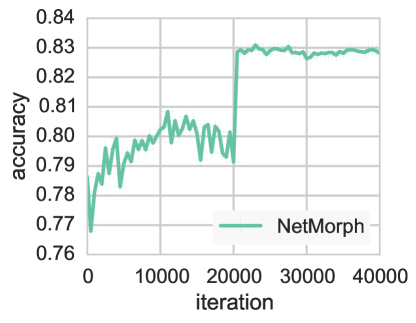
In this section we evaluate kernel size morphing and width morphing in the sequence of cifar_base$\to$ksize$\to$width. The detailed network architectures are shown in Table 1. The baseline network (cifar_base) is a narrower version of cifar_222 with an accuracy of 81.48%.

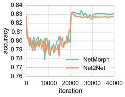
Fig. 9(a) shows the curve of kernel size morphing, which expands the kernel size of the second layer in each subnet from 1 to 3 (cifar_ksize). This results in a performance of 82.81%, which is 1.33% higher than the parent network. We further double the number of channels (width) for the first layer in each subnet (cifar_width). Fig. 9(b) shows the results of NetMorph and Net2Net. As can be seen, NetMorph is slightly better. It improves the performance to 83.09% while Net2Net dropped a little to 82.70%.

For width morphing, NetMorph works for arbitrary continuous non-linear activation functions, while Net2Net only for piece-wise linear ones. We also conducted width morphing directly from the parent network for TanH neurons, which results in about 4% accuracy improvement.

4.4 Experiment on ImageNet

We also conduct experiments on the ImageNet dataset (Russakovsky et al., 2014) with 1,000 object categories. The models were trained on 1.28 million training images and tested on 50,000 validation images. The top-1 and top-5 accuracies for both 1-view and 10-view are reported.

The proposed experiments is based on the VGG16 net, which was actually trained with multi-scales (Simonyan & Zisserman, 2014). Because the Caffe (Jia et al., 2014) implementation favors single-scale, for a fair comparison, we first de-multiscale this model by continuing to train it on the ImageNet dataset with the images resized to $256\times 256$. This process caused about 1% performance drop. This coincides with Table 3 in (Simonyan & Zisserman, 2014) for model D. In this paper, we adopt the de-multiscaled version of the VGG16 net as the parent network to morph. The morphing operation we adopt is to add a convolutional layer at the end of the first three subsets for each. The detailed network architecture is shown in Table 2. We continue to train the child network after morphing, and the final model is denoted as VGG16(NetMorph). The results are shown in Table 3. We can see that, VGG16(NetMorph) not only outperforms its parent network, i.e, VGG16(baseline), but also outperforms the multi-scale version, i.e, VGG16(multi-scale). Since VGG16(NetMorph) is a 19-layer network, we also list the VGG19 net in Table 3 for comparison. As can be seen, VGG16(NetMorph) also outperforms VGG19 in a large margin. Note that VGG16(NetMorph) and VGG19 have different architectures, as shown in Table 2. Therefore, the proposed NetMorph scheme not only can help improve the performance, but also is an effective network architecture explorer. Further, we are able to add more layers into VGG16(NetMorph), and a better performing model shall be expected.

We compare the training time cost for the NetMorph learning scheme and the training from scratch. VGG16 was trained for around 2~3 months for a single GPU time (Simonyan & Zisserman, 2014), which does not include the pre-training time on a 11-layered network. For a deeper network, the training time shall increase. While for the 19-layered network VGG16(NetMorph), the whole morphing and training process was finished within 5 days, resulting in around 15x speedup.

Table 3: Comparison results on ImageNet.

	Top-1	Top-5	Top-1	Top-5
	1-view	1-view	10-view	10-view
VGG16 (multi-scale)	68.35%	88.45%	69.59%	89.02%
VGG19 (multi-scale)	68.48%	88.44%	69.44%	89.21%
VGG16 (baseline)	67.30%	88.31%	68.64%	89.10%
VGG16 (NetMorph)	69.14%	89.00%	70.32%	89.86%

5 Conclusions

In this paper, we have introduced the systematic study about network morphism. The proposed scheme is able to morph a well-trained parent network to a new child network, with the network function completely preserved. The child network has the potential to grow into a more powerful one in a short time. We introduced diverse morphing operations, and developed novel morphing algorithms based on the morphism equations we have derived. The non-linearity of a neural network has been carefully addressed, and the proposed algorithms enable the morphing of any continuous non-linear activation neurons. Extensive experiments have been carried out to demonstrate the effectiveness of the proposed network morphism scheme.

References

- Ba & Caruana (2014) Ba, Jimmy and Caruana, Rich. Do deep nets really need to be deep? In Advances in Neural Information Processing Systems, pp. 2654–2662, 2014.
- Bishop (2006) Bishop, Christopher M. Pattern recognition. Machine Learning, 2006.
- Bucilu et al. (2006) Bucilu, Cristian, Caruana, Rich, and Niculescu-Mizil, Alexandru. Model compression. In Proceedings of the 12th ACM SIGKDD International Conference on Knowledge Discovery and Data Mining, pp. 535–541. ACM, 2006.
- Chang & Chen (2015) Chang, Jia-Ren and Chen, Yong-Sheng. Batch-normalized maxout network in network. arXiv preprint arXiv:1511.02583, 2015.
- Chen et al. (2015) Chen, Tianqi, Goodfellow, Ian, and Shlens, Jonathon. Net2net: Accelerating learning via knowledge transfer. arXiv preprint arXiv:1511.05641, 2015.
- Girshick (2015) Girshick, Ross. Fast r-cnn. arXiv preprint arXiv:1504.08083, 2015.
- Girshick et al. (2014) Girshick, Ross, Donahue, Jeff, Darrell, Trevor, and Malik, Jagannath. Rich feature hierarchies for accurate object detection and semantic segmentation. In IEEE Conference on Computer Vision and Pattern Recognition, pp. 580–587. IEEE, 2014.
- Glorot & Bengio (2010) Glorot, Xavier and Bengio, Yoshua. Understanding the difficulty of training deep feedforward neural networks. In International Conference on Artificial Intelligence and Statistics, pp. 249–256, 2010.
- He et al. (2015a) He, Kaiming, Zhang, Xiangyu, Ren, Shaoqing, and Sun, Jian. Deep residual learning for image recognition. arXiv preprint arXiv:1512.03385, 2015a.
- He et al. (2015b) He, Kaiming, Zhang, Xiangyu, Ren, Shaoqing, and Sun, Jian. Delving deep into rectifiers: Surpassing human-level performance on imagenet classification. arXiv preprint arXiv:1502.01852, 2015b.
- Jia et al. (2014) Jia, Yangqing, Shelhamer, Evan, Donahue, Jeff, Karayev, Sergey, Long, Jonathan, Girshick, Ross, Guadarrama, Sergio, and Darrell, Trevor. Caffe: Convolutional architecture for fast feature embedding. In Proceedings of the ACM International Conference on Multimedia, pp. 675–678. ACM, 2014.
- Krizhevsky & Hinton (2009) Krizhevsky, Alex and Hinton, Geoffrey. Learning multiple layers of features from tiny images, 2009.
- Krizhevsky et al. (2012) Krizhevsky, Alex, Sutskever, Ilya, and Hinton, Geoffrey E. Imagenet classification with deep convolutional neural networks. In Advances in Neural Information Processing Systems, pp. 1097–1105, 2012.
- LeCun et al. (1998) LeCun, Yann, Bottou, Léon, Bengio, Yoshua, and Haffner, Patrick. Gradient-based learning applied to document recognition. Proceedings of the IEEE, 86(11):2278–2324, 1998.
- Lin et al. (2013) Lin, Min, Chen, Qiang, and Yan, Shuicheng. Network in network. CoRR, abs/1312.4400, 2013. URL http://arxiv.org/abs/1312.4400.
- Long et al. (2014) Long, Jonathan, Shelhamer, Evan, and Darrell, Trevor. Fully convolutional networks for semantic segmentation. arXiv preprint arXiv:1411.4038, 2014.
- Oquab et al. (2014) Oquab, Maxime, Bottou, Leon, Laptev, Ivan, and Sivic, Josef. Learning and transferring mid-level image representations using convolutional neural networks. In IEEE Conference on Computer Vision and Pattern Recognition, pp. 1717–1724. IEEE, 2014.
- Ren et al. (2015) Ren, Shaoqing, He, Kaiming, Girshick, Ross, and Sun, Jian. Faster r-cnn: Towards real-time object detection with region proposal networks. In Advances in Neural Information Processing Systems, pp. 91–99, 2015.
- Romero et al. (2014) Romero, Adriana, Ballas, Nicolas, Kahou, Samira Ebrahimi, Chassang, Antoine, Gatta, Carlo, and Bengio, Yoshua. Fitnets: Hints for thin deep nets. arXiv preprint arXiv:1412.6550, 2014.
- Russakovsky et al. (2014) Russakovsky, Olga, Deng, Jia, Su, Hao, Krause, Jonathan, Satheesh, Sanjeev, Ma, Sean, Huang, Zhiheng, Karpathy, Andrej, Khosla, Aditya, Bernstein, Michael, et al. Imagenet large scale visual recognition challenge. International Journal of Computer Vision, pp. 1–42, 2014.
- Simonyan & Zisserman (2014) Simonyan, Karen and Zisserman, Andrew. Very deep convolutional networks for large-scale image recognition. arXiv preprint arXiv:1409.1556, 2014.
- Szegedy et al. (2014) Szegedy, Christian, Liu, Wei, Jia, Yangqing, Sermanet, Pierre, Reed, Scott, Anguelov, Dragomir, Erhan, Dumitru, Vanhoucke, Vincent, and Rabinovich, Andrew. Going deeper with convolutions. arXiv preprint arXiv:1409.4842, 2014.
- Weisstein (2002) Weisstein, Eric W. CRC concise encyclopedia of mathematics. CRC press, 2002.