Learning deep representation of multityped objects and tasks

Abstract

We introduce a deep multitask architecture to integrate multityped representations of multimodal objects. This multitype exposition is less abstract than the multimodal characterization, but more machine-friendly, and thus is more precise to model. For example, an image can be described by multiple visual views, which can be in the forms of bag-of-words (counts) or color/texture histograms (real-valued). At the same time, the image may have several social tags, which are best described using a sparse binary vector. Our deep model takes as input multiple type-specific features, narrows the cross-modality semantic gaps, learns cross-type correlation, and produces a high-level homogeneous representation. At the same time, the model supports heterogeneously typed tasks. We demonstrate the capacity of the model on two applications: social image retrieval and multiple concept prediction. The deep architecture produces more compact representation, naturally integrates multiviews and multimodalities, exploits better side information, and most importantly, performs competitively against baselines.

Keywords: Deep representation learning; multityped objects; multityped tasks; multimodal learning; multitask learning

1 Introduction

Image	Caption	Tags	Comments	Groups
	i am moving	leaves, snail, slow, evening, movement, animal, crust, nikon, d5100, srilanka, beautiful, art, asiasociety, image, photo, interesting, green, mail, wait, ambition, colour, depth, bokeh	[amazing shot!, fabulous macro]; [awesome shot! what an amazing little creature!]	[insects, spiders, snails and slugs]; [fotógrafos anônimos]
	leaves and dew	dew, nikon, d5100, srilanka, beautiful, art, asiasociety, image, photo, interesting, morning, sun, sunlight, background, green	excellent light and beautiful tones against the black background, uditha!!!	[fotógrafos anônimos]
	purple-rumped sunbird	bird, nikon, d5100, srilanka, beautiful, art, asiasociety, image, photo, interesting, photography, sunbird, purplerumpedsunbird, branch, stance, wild, garden	a beautiful looking bird. well captured. congrats.	[birds]; [555]
	wish you all happy 2015.	sunrise, newyear, nikon, d5100, srilanka, beautiful, art, asiasociety, sun morning, leave, leaves, new, 2015, horizon, hospital, sunspots, badulla, uva, year, rise, rising	wow! excellent shot! happy year!!!	[monochrome (color only!)]; [fotógrafos anônimos]

Figure 1: Flickr images: captions, tags, comments and groups. The visual modality can has multiple representations, including a variety of histograms and bag of visual words. Photos by uditha wickramanayaka.

Multimedia objects instantly command our attention. Yet they are notoriously difficult to model. Multimedia objects require fusing multiple modalities of distinct characteristics with wide semantic gaps. An online image, for example, could be associated with human-level semantics such as captions, tags, comments, sentiments and the surrounding context. The image itself, however, has pixels and colors arranged in a 2D grid – a machine-level representation (see Fig. 1 for examples). To construct more meaningful abstraction, a visual image can be represented in multiple ways including several histograms of color, edge, texture; and a bag of visual words (BOW) [7].

A common approach to learning from multiple representations is to concatenate all features and form a long flat vector, assuming that representations are equally informative. This is likely to cause problems for several reasons. First there is a high variation in dimensionality and scales between types (e.g., histogram vectors are often dense and short while BOW vector is sparse and long). Second, modalities have different correlation structures that warrant separate modeling [26]. A single modality can also admit multiviews, hence multiple types. For the visual modality, a histogram is a real-valued vector but a bag of visual words is a discrete set of word counts. Thus effective modeling should also account for type-specific properties. Type modeling is, however, largely missing in prior multimodal research [3, 17, 19]. To better address multimodal differences in correlation structures, it is necessary to recognize that intra-mode correlation is often much higher than inter-mode correlation [17]. This suggests a two step fusion. Translated to typed representations, we need to first decorrelate the intra-type data, then capture the inter-type inter-dependencies.

While modeling multityped multimodality is essential to capture the intra/inter-type correlation structure, care must be paid for the tasks at hand. Representations that are handcrafted independent of future tasks are likely to be suboptimal. This suggests task-informed representation learning. Putting together, we argue that a more successful approach should work across tasks, modalities, semantic levels and coding types.

To this end, this paper introduces a bottom-up deep learning approach to tackle the challenges. Deep architectures [13, 20, 31] offer a natural solution for decoupling the intra-type correlation from the inter-type correlation through multiple layers [17, 26]. Starting from the bottom with machine-friendly representations, each object is characterized by a collection of type-specific feature vectors, where each type is a homogeneous numerical or qualitative representation such as real-valued, binary, or count. These primitive representations enable each modality to be expressed in more than one way, each of which may belong to a type. For example, the visual modality of an image can be represented by one or more real-valued color histograms or a bag of word counts, and its social tags can be considered as a sparse binary vector. The intra-type correlation is handled by type-specific lower models. Moving up the hierarchy, inter-type correlation is captured in a higher layer. And finally, tasks are defined on top of the higher layer.

(A) Restricted Boltzmann machine	(B) Layerwise training	(C) Multitask multityped refinement

Figure 2: A $3$-step training procedure: (A) First type-specific RBMs are trained; (B) then posteriors of the previous layers are used as the input for the next layer; (C) finally auxiliary tasks are learnt, refining the previously discovered latent representation. Steps A, B are unsupervised and Step C is supervised.

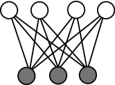
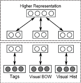
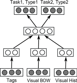
Our realization of this deep learning scheme is a two-phase procedure based on a stack of restricted Boltzmann machines (RBMs) [25, 32], as depicted in Fig. 2. The first learning phase is unsupervised. It discovers data regularities and the shared structures between modalities and types without labels. Learning starts from the lowest level, where an array of RBMs map the type-specific inputs into intermediate representations. These middle-level representations are then integrated by another binary RBM into high-level features. The stack forms a multityped deep belief network [13]. In the second learning phase, auxiliary typed tasks are introduced on top of the highest feature layer, essentially forming a multityped deep neural network. The tasks are learnt simultaneously and the previously learnt representations are refined in the process. This creates a more predictive deep representation shared among tasks [4]. Our approach appears to resemble recent multimodal multitask learning frameworks [36, 33]. However, we differ significantly by modeling types at both the input and the task levels, while previous work often assumes homogeneous representations.

To summarize, this paper makes the following contributions:

• Introduction of a deep multityped architecture to integrate multiviews and multimodalities.

• Introducing the concept of multityped multitask learning, where tasks are heterogeneous in types.

• An evaluation of the proposed architecture on the NUS-WIDE data [7], demonstrating its capacity on two applications: image retrieval and multilabel concept learning.

The next section reviews related background. Section 3 presents the building blocks of the proposed architecture – restricted Boltzmann machines. The deep architecture for multityped inputs and tasks is described in Section 4. Section 5 demonstrates the applicability of the proposed deep architecture on two applications: image retrieval and multilabel learning. Finally, Section 6 concludes the paper.

2 Related background

Learning from multimodal data has recently attracted an increasing attention [17, 19, 8, 11, 18, 35]. However, the fusion of multiple data types is sparsely studied. Early attempts include the work of [3], where a joint probabilistic model, the correspondence latent Dirichlet allocation (LDA), was proposed. The model explicitly assumes the direct correspondence in the data (i.e., which image region generates which labels). A more recent work [19] uses LDA to model text and image features. Modalities are treated as two separate sources which are lately fused using canonical correlation analysis. It is, however, not clear to how systematically handle different data types and more than two sources.

Our work extends a rich class of undirected graphical models known as restricted Boltzmann machines (RBMs) [25], capable of encoding arbitrary types and side information [28, 27]. Most existing work in RBMs is limited to single types, for example, binary [25], real-valued [13] or count [22]. Joint modelling of visual features and tags was first introduced in [34]. This line of work was extended further in [28, 27] with a richer set of types. These works, however, assume a shallow architecture which may not be ideal for multimedia objects, where modalities differ substantially in their correlation structures and semantic levels [17].

More recently, deep architectures have been suggested to overcome the difficulties associated with the shallow models in multimodal learning. The deep canonical correlation analysis [2], for example, can potentially help narrow the semantic gaps. Multimodal stacked autoencoders have been shown to be effective for integrating speech and vision [17]. These efforts, however, do not address multiple data types. Closer to our architecture is perhaps the work of [26], where a deep Boltzmann machine [20] is used for multimodal data. The key differences are that the work of [26] assumes each modality has only one view (and type), and the model is purely generative. Our work, on the other hand, extends to multiple views and multiple types per modality, with both the generative and discriminative components. Multiple views (and types) from the same visual modality has been studied in [15], but this is limited to hashing and does not consider multityped tasks.

Neural networks for multitask learning was first introduced in [5]. Exploiting auxiliary tasks with shared latent representation to improve the main task has been previously proposed [1]. Multimodal multitask learning has been studied in [36, 33]. However, we differ significantly by modeling heterogeneous types at both the input and task levels, while the previous work often assumes homogeneous representations.

3 Sparse restricted Boltzmann machines

We first present building blocks for our deep architecture – the restricted Boltzmann machine (RBM) and its generalizations. A restricted Boltzmann machine is a stochastic undirected neural network without outputs [25, 32] (see Fig. 2(A) for a graphical depict). Given binary inputs $\boldsymbol{v}\in\left\{0,1\right\}^{N}$ and hidden units $\boldsymbol{h}\in\left\{0,1\right\}^{K}$, the RBM defines the following energy function:

$$E(\boldsymbol{v},\boldsymbol{h})=-\sum_{i=1}^{N}a_{i}v_{i}-\sum_{k=1}^{K}b_{k}h_{k}-\sum_{i=1}^{N}\sum_{k=1}^{K}W_{ik}v_{i}h_{k}$$ (1)

where $a_{i},b_{k}$ are biases and $W_{ik}$ is the weight of the interaction between an input unit $i$ and a hidden unit $k$.

Unlike traditional neural networks, the RBM does not map inputs into outputs, but rather, models a joint multivariate distribution as follows:

$$P(\boldsymbol{v},\boldsymbol{h})=\frac{1}{Z}\exp\left(-E(\boldsymbol{v},\boldsymbol{h})\right)$$

where $Z$ is the normalizing constant. The RBM’s bipartite structure (Fig. 2a) posits the following factorizations

$$P(\boldsymbol{v}\mid\boldsymbol{h}) = \prod_{i=1}^{N}P(v_{i}\mid\boldsymbol{h});\quad P(\boldsymbol{h}\mid\boldsymbol{v})=\prod_{k=1}^{K}P(h_{k}\mid\boldsymbol{v})$$ (2)

where

$$P(v_{i} =1\mid\boldsymbol{h})=\sigma\left[a_{i}+\sum_{k=1}^{K}W_{ik}h_{k}\right]$$ (3)

$$P(h_{k} =1\mid\boldsymbol{v})=\sigma\left[b_{k}+\sum_{i=1}^{N}W_{ik}v_{i}\right]$$ (4)

where $\sigma[z]=1/(1+e^{-z})$ is the sigmoid function. The posterior vector $\left(\bar{h}_{1},\bar{h}_{2},...,\bar{h}_{K}\right)$ where $\bar{h}_{k}=P(h_{k}=1\mid\boldsymbol{v})$ serves as a new representation of the data. The factorizations in Eq. (2) enable efficient layerwise MCMC sampling by alternating between $\hat{\boldsymbol{v}}\sim P(\boldsymbol{v}\mid\boldsymbol{h})$ and $\hat{\boldsymbol{h}}\sim P(\boldsymbol{h}\mid\boldsymbol{v})$.

Parameters $\boldsymbol{\theta}=\left\{a_{i},b_{k},W_{ik}\right\}$ are typically estimated by maximizing the data likelihood $P(\boldsymbol{v})$. To encourage sparse representation, that is, the low probability that a hidden unit is activated, we augment the data log-likelihood with a regularization term:

$$\boldsymbol{\theta}^{*}=\arg\max_{\boldsymbol{\theta}}\left(\log P(\boldsymbol{v})+\gamma\sum_{k}q_{k}\bar{h}_{k}\right)$$

where $q_{k}\ll 1$ is the desired activation probability of the $k$-th hidden unit, and $\gamma>0$ is regularization factor. Learning can be realized through a fast stochastic gradient ascent procedure known as contrastive divergence [12]:

$$W_{ik} \leftarrow W_{ik}+\eta\left(v_{i}\bar{h}_{k}-\bar{v}_{i}\hat{h}_{k}\right)+\gamma v_{i}\left(q_{k}-\bar{h}_{k}\right)$$ (5)

$$b_{k} \leftarrow b_{k}+\eta\left(\bar{h}_{k}-\hat{h}_{k}\right)+\gamma\left(q_{k}-\bar{h}_{k}\right)$$ (6)

$$a_{i} \leftarrow a_{i}+\eta\left(v_{i}-\bar{v}_{i}\right)$$ (7)

where $\eta>0$ is learning rate, $\bar{v}_{i}=P(v_{i}=1\mid\hat{\boldsymbol{h}})$, and $\hat{\boldsymbol{h}}$ is a sample drawn from a short MCMC run starting from the input $\boldsymbol{v}$. This procedure approximately maximizes the data likelihood $P(\boldsymbol{v})$.

A major limitation of RBM is that it can only model binary inputs. In the next subsections, we present extensions for real-valued inputs with Gaussian-Bernoulli RBM [13] and count inputs with constrained Poisson RBM [22].

3.1 Gaussian–Bernoulli RBM

Gaussian–Bernoulli RBMs model real–valued inputs such as pixel intensities and histograms [13]. The graphical structure is exactly the same that of standard RBMs (Fig. 2(A)), except for the input type, where $\boldsymbol{v}\in\mathbb{R}^{N}$. The energy in Eq. (1) is replaced by:

$$E(\boldsymbol{v},\boldsymbol{h})=\frac{1}{2}\sum_{i=1}^{N}\left(v_{i}-a_{i}\right)^{2}-\sum_{k=1}^{K}b_{k}h_{k}-\sum_{i=1}^{N}\sum_{k=1}^{K}W_{ik}v_{i}h_{k}$$

Here for simplicity, we have assumed unit variance for each input variable. Like the binary case, the factorizations in Eq. (2) still hold. The posterior $P(h_{k}\mid\boldsymbol{v})$ assumes the same form as in Eq. (4). However, the generative distribution $P(v_{i}\mid\boldsymbol{h})$ now follows a normal distribution of variance $1$ and mean:

$$\mu_{i}(\boldsymbol{h})=a_{i}+\sum_{k=1}^{K}W_{ik}h_{k}$$ (8)

Learning in the Gaussian–Bernoulli RBMs can also be done using the stochastic procedure as in Eqs. (5–7) with a modification: $\bar{v}_{i}=\mu_{i}(\boldsymbol{h})$.

3.2 Constrained Poisson RBM

Counts as in bag-of-words representation can be modeled using an approximate constrained Poisson model [22]. Let $\boldsymbol{v}\in\left\{0,1,2,...\right\}^{N}$, the model energy reads

$$E(\boldsymbol{v},\boldsymbol{h})=\sum_{i=1}^{N}\left(\log\left(v_{i}!\right)-a_{i}v_{i}\right)-\sum_{k=1}^{K}b_{k}h_{k}-\sum_{i=1}^{N}\sum_{k=1}^{K}W_{ik}v_{i}h_{k}$$

The factorizations in Eq. (2) still hold and does the posterior $P(h_{k}\mid\boldsymbol{v})$ in Eq. (4). However, the generative distribution $P(v_{i}\mid\boldsymbol{h})$ now admits a constrained Poisson distribution:

$$P(v_{i}=n\mid\boldsymbol{h})=\mbox{Poisson}\left(n,\lambda_{i}(\boldsymbol{h})\right)$$

where $\lambda_{i}(\boldsymbol{h})$ is the mean–rate, calculated as

$$\lambda_{i}(\boldsymbol{h})=M\frac{\exp\left(\mu_{i}(\boldsymbol{h})\right)}{\sum_{j=1}^{N}\exp\left(\mu_{j}(\boldsymbol{h})\right)}$$

where $M=\sum_{i}v_{i}$ is document length and $\mu_{i}(\boldsymbol{h})$ is given in Eq. (8). This special mean–rate ensures that $\sum_{i}\lambda_{i}(\boldsymbol{h})=M$, i.e., $\lambda_{i}(\boldsymbol{h})$ is bounded from above. In addition, the model rate equals the empirical rate, on average, leading to more stable learning.

Learning in the constrained Poisson RBMs using the stochastic procedure as in Eqs. (5–7) requires only a minimum change: $\bar{v}_{i}=\lambda_{i}(\boldsymbol{h})$.

3.3 Other RBM types

RBMs have been extended to other types including multinomial [23], ordinal [29], rank [28], beta [16] and a mixture of these [28]. As with real-valued and count types, these extensions maintain the same bipartite structure of the RBMs, only differ in type-specific generative distributions $P(v_{i}\mid\boldsymbol{h})$. A recent flexible framework in [27] is claimed to represent most known types using truncated Gaussian–Bernoulli RBMs. Here there are two hidden layers rather than one and the real-valued layer is constrained through type-specific inequalities.

4 A deep architecture for multityped representations and tasks

We now present the deep architecture for multityped objects and multityped tasks. Our learning is a $3$-step procedure spanning over an unsupervised learning phase and a supervised phase, as depicted in Figs. 2 (A), (B) and (C), respectively. The key ideas are two-fold: (i) separation of modeling of intra-type correlation from inter-type correlation using multiple layers, and (ii) using predictive tasks to refine the learnt representation.

4.1 Learning procedure

We derive a 2-phase learning procedure. The first phase is unsupervised where representations are learnt from the data without guidance from any labels. The second phase is supervised where the tasks are used to fine-tune the previously learnt model.

Phase 1: Unsupervised learning

This phase has two steps, one is to model intra-type correlation and the other is to decouple inter-type correlation.

• Step A – Learning type-specific representations: We first ignore the inter-type correlation and each feature set is modeled separately using a type-specific RBM. Let us assume that each object can be represented by $S$ ways, each of which corresponds to a feature set $\boldsymbol{v}_{s}$, for $s=1,2,..,S$. At the end of the step, we have $S$ set of posteriors $\hat{\boldsymbol{h}}_{s}=\left(\hat{h}_{s1},\hat{h}_{s2},..,\hat{h}_{sN_{s}}\right)$, where $\hat{h}_{sk}=P(h_{sk}=1\mid\boldsymbol{v}_{s})$ for $s=1,2,...,S$. This new representation is expected to reduce the intra-type correlation.

• Step B – Learning joint representation: We now model the inter-type correlation (e.g., see the upper half of Fig. 2(B)). The posteriors of type-specific RBMs for each object are concatenated as an input for another binary RBM, i.e., $\boldsymbol{v}^{(2)}\leftarrow\left[\hat{\boldsymbol{h}}_{1}^{(1)}\mid\hat{\boldsymbol{h}}_{2}^{(1)}\mid...\mid\hat{\boldsymbol{h}}_{S}^{(1)}\right]$. The posterior in this second stage $P(\boldsymbol{h}^{(2)}\mid\boldsymbol{v}^{(2)})$ is expected to be more abstract than those in the first stage. This step has been shown to improve the lower-bound of the data log-likelihood: $P(\boldsymbol{v})$ [13].

Phase 2: Supervised fine-tuning

• Step (C) – Learning tasks-informed representations: The two layers from Steps A and B are now connected by joining the output of the first layer and the input of the second layer, as depicted in Fig. 2(C). Essentially, the joint model becomes a generalization of the deep belief network [13] where the input is multityped. Further, the top hidden layer is connected to tasks of interest. The whole model is now a complex deep neural network which supports multiple input types as well as multiple output tasks. Finally, the parameters are refined by discriminative training of tasks through back-propagation. We elaborate this step further in the following subsection.

4.2 Multityped multitask learning

Let $\boldsymbol{b}_{s}^{(1)},\boldsymbol{W}_{s}^{(1)}$ denote the parameters associated with the $s$-th feature set at the bottom layer, and $\boldsymbol{b}^{(2)},\boldsymbol{W}^{(2)}$ be the parameters of the second layer. At the end of Step B, the $k$-th higher feature can be computed in a feedforward procedure:

$$f_{k}(\boldsymbol{v}_{1:S}) = \sigma\left[b_{k}^{(2)}+\sum_{s}\sum_{m}W_{smk}^{(2)}\sigma\left[b_{sm}^{(1)}+\sum_{i}W_{sim}^{(1)}v_{si}\right]\right]$$ (9)

where $\sigma$ is the sigmoid function. These learned representations can then be used for future tasks such as retrieval, clustering or classification.

However, learning up to this point has been aimed to approximately optimize the lower-bound of the data likelihood $P(\boldsymbol{v}_{1:S})$ [13]. Since the data likelihood may not be well connected with the tasks we try to perform, using the discovered representation at the second stage may be suboptimal. A more informative way is to guide the learning process so that the learned representation become predictive with respect to future tasks. Beside the main tasks of interest, we argue that auxiliary tasks can be helpful the shape the representations. This provides a realization of Vapnik’s idea of learning with privileged information [30] in that the teacher knows extra information (auxiliary tasks) that is only available at training time. For example, if the main task is content-based retrieval or concept labeling, ranking social tags associated with images can be used as an auxiliary task. On absence of well-defined extra tasks, we can use input reconstruction as auxiliary tasks. Note that the auxiliary tasks (and side information) are only needed at training time.

The major distinctive aspect of our multitask setting is that tasks are multityped, that is, tasks do not assume the same functional form. For example, one task can be histogram reconstructions through regression, the other can be tagging through label ranking. The tasks, however, share the same latent data representation, along the line of [5]. As the model is now a deep neural network, the standard back-propagation applies. The major difference is now the parameters learnt from the unsupervised phase serve as initialization for the supervised phase. Numerous evidences in the literature suggest that this initialization is in a sensible parameter region, enabling exploitation of good local minima, and at the same time, implicitly provides regularization [13, 10].

We consider two task categories, one with a single outcome per task (unstructured outputs), and the other with composite outcome (structured outputs).

4.2.1 Unstructured outputs

Let $y_{t}$ be the outcome for the $t$-th task and

$$g_{t}(\boldsymbol{v}_{1:S})=V_{t0}+\sum_{k}V_{tk}f_{k}(\boldsymbol{v}_{1:S})$$

where $f_{k}(\boldsymbol{v}_{1:S})$ are top-level features computed in Eq. (9). We then refine the model by optimizing loss functions with respect to all parameters $\boldsymbol{c},\boldsymbol{V},\boldsymbol{W}^{(1)},\boldsymbol{W}^{(2)},\boldsymbol{b}_{1:S}^{(1)}$ and $\boldsymbol{b}^{(2)}$. Examples of task types and associated loss functions are:

• Regression for real-valued outcomes. For $y_{t}\in\mathbb{R}$, the loss function is:

  $$L_{t}=\frac{1}{2}\left(y_{t}-g_{t}(\boldsymbol{v}_{1:S})\right)^{2}$$ (10)

• Logistic regression for binary outcomes. For $y_{t}\in\pm 1$, the loss function has a log-form:

  $$L_{t}=\log\left(1+\exp\left(-y_{t}g_{t}(\boldsymbol{v}_{1:S})\right)\right)$$ (11)

• Poisson regression for counts. For $y_{t}=0,1,2,..$, the loss function is negative log of the Poisson distribution:

  $$L_{t}=\log(y_{t}!)-y_{t}\log\lambda_{t}+\lambda_{t}$$ (12)

  where $\lambda_{t}=e^{g_{t}(\boldsymbol{v}_{1:S})}$ is the mean-rate. Since the first term $\log(y_{t}!)$ is a constant with respect to model parameters, it can be ignored during learning.

4.2.2 Structured outputs

We consider three cases, namely multiclass prediction, (partial) label ranking and multilabel learning. Label ranking refers to the ordering of labels according to their relevance with respect to an object. For example, for an image, the ranking of the groups to which the image belong may be: {birds $\succ$ close-up $\succ$ outdoor $\succ$ indoor}. Partial label ranking is when the rank given is incomplete, e.g., only the {birds $\succ$ close-up $\succ$ others} is given. When only one label is known, this reduces to the multiclass problem. Multilabel prediction is to assign more than one label for each object. The same above image can be tagged as {bird, morning, branch, wild, garden}, for example.

Let $\left\{y_{t1},y_{t2},...,y_{tT_{t}}\right\}$ be the $T_{t}$ labels given to the object in the $t$-th task. Here we employ a simple strategy: A label is chosen with the following probability:

$$P_{j}\left(y_{tj}=l\mid\boldsymbol{v}_{1:S}\right)=\frac{\exp\left\{V_{tl}+\sum_{k}V_{tlk}f_{k}(\boldsymbol{v}_{1:S})\right\}}{\sum_{l^{\prime}\in\mathcal{L}_{j}}\exp\left\{V_{tl^{\prime}}+\sum_{k}V_{tl^{\prime}k}f_{k}(\boldsymbol{v}_{1:S})\right\}}$$ (13)

where $\mathcal{L}_{j}$ is a set consisting of $y_{tj}$ and other labels that are deemed equal or better than the $j$-th outcome. The loss function is

$$L_{t}=-\sum_{j=1}^{T_{t}}\log P_{j}\left(y_{tj}=l\mid\boldsymbol{v}_{1:S}\right)$$

The three specific cases are:

• For multiclass prediction, $\mathcal{L}_{1}$ has all class labels and $T_{t}=1$.

• For (partial) label ranking, $\mathcal{L}_{1}$ consists of all labels and $\mathcal{L}_{j}$ is defined recursively as follows $\mathcal{L}_{j}=\mathcal{L}_{j-1}\backslash y_{tj}$. This essentially reduces to the Plackett-Luce model when complete ranking is available [6]. Prediction is simple as we need to rank all the labels according to $P_{j}\left(y_{tj}=l\mid\boldsymbol{v}_{1:S}\right)$.

• For multilabel learning, $\mathcal{L}_{j}$ contains all labels for $j=1,2,..,T_{t}$. For prediction, we adapt the strategy in [9] in that only those labels satisfying $P(y\mid\boldsymbol{v}_{1:S})\geq\tau(\boldsymbol{v}_{1:S})$ are selected. The threshold $\tau(\boldsymbol{v}_{1:S})$ is a function of $\left\{P_{j}\left(y_{tj}=l\mid\boldsymbol{v}_{1:S}\right)\right\}_{j=1}^{T_{t}}$ which is estimated from the training data by maximizing an objective of interest. In our setting, the objective is the label-wise $F$-score.

5 Experiments

We evaluate our learning method on the NUS-WIDE dataset [7]. This consists of more than $200K$ Flickr images, each of which is equipped with (1) $6$ visual feature representations (64-D color histogram, 144-D color correlogram, 73-D edge direction histogram, 128-D wavelet texture, 225-D block-wise color moments, and 500-D BOWs from SIFT descriptors), (2) tags drawn from a $5$K-word vocabulary, and (3) one or more of $81$ manually labelled concepts. We randomly pick $10,000$ images for training our model and $10,000$ for testing. The dimensionality of the social tags is limited to $1000$. For BOWs, we use $\left(\left[\log(1+\mbox{count})\right]\right)$ instead of count. For real-valued histograms, we first normalize each histogram to an unit vector, then normalize them across all train data to obtain zero mean and unit variance.

Our model architecture has $200$ hidden units per type at the bottom layer, and $200$ hidden units at the top layer. Mapping parameters $\boldsymbol{W}$ are randomly initialized from small normally distributed numbers, and bias parameters $\boldsymbol{b}$ are from zeros. Posterior sparsity $q_{k}$ is set to $0.2$ (see Eq. (5)). Learning rates are set at $0.1$ for binary, $0.01$ for real-valued and $0.02$ for count types. The difference in learning rate scales is due to the fact that real-valued Gaussian means are unbounded, and Poisson mean–rates, although bounded, may be larger than 1. Parameters in the unsupervised phase (Steps A,B) are updated after every $100$ training images. The discriminative training in the supervised phase (Step C) is based on back-propagation and conjugate gradients.

5.1 Image retrieval

In this task, each test image is used to query other test objects. Retrieval is based on the cosine similarity between representations of the query and the objects. For our deep architecture, the top-level representation is used, where each unit is $f_{k}(\boldsymbol{v}_{1:S})$ as in Eq. (9). To create a baseline representation, we first normalize each feature set to a unit vector before concatenating them. This eliminates the difference in dimensionality and scales between views. A retrieved image is considered relevant if it shares at least one manually labelled concept with the query.

Features$\rightarrow$ Auxiliary Tasks	Input types	Output types
500D-BOW$\rightarrow$ Tags	Count	Multilabel
64D-CH$\rightarrow$ Tags	Real	Multilabel
1134D-Visual$\rightarrow$Tags	Real & count	Multilabel
1134D-Visual$\rightarrow$(Visual & Tags)	Real & count	Real, count & multilabel
(64D-CH & Tags)$\rightarrow$ Tags	Real & bin	Multilabel

Table 1: Type definitions for retrieval. (Features$\rightarrow$ Aux. Tasks) means auxiliary tasks are used to fine-tune the model given the features. 64D-CH means the 64 bin color histogram, 1134D-Visual means all 6 visual features combined.

Auxiliary tasks are used in the training phase but not in the testing phase. If the input is purely visual, then this reduces to content-based image retrieval [24]. We test two settings with the auxiliary tasks, where we predict either tags (tagging) or combination of visual features and tags (feature reconstruction & tagging). The task types are defined as follows (see also Tab. 1):

• Tagging as a multilabel prediction problem (Sec. 4.2.2).

• Histogram reconstruction as multiple regressions (Eq. (10)).

• BOW reconstruction as multiple Poisson regressions (Eq. (12)).

5.1.1 Performance measures

Two performance measures are reported: Mean Average Precision (MAP) over the top $100$ retrieved images, and the Normalized Discounted Cumulative Gain (NDCG) [14] at the top $10$ images. Let $\mbox{rel}_{i}\in\left\{0,1\right\}$ denote whether the $i$-th retrieved image is relevant to the query. The precision at rank $n$ is $\mbox{Precision}(n)=\frac{1}{n}\sum_{i=1}^{n}\mbox{rel}_{i}$. The MAP is computed as follows:

MAP $$=\frac{1}{Q}\sum_{q=1}^{Q}\frac{1}{T}\sum_{n=1}^{T}\mbox{Precision}_{q}(n)$$

where $Q=10,000$ is the number of test queries, and $T=100$ is the number of top images.

The Discounted Cumulative Gain (DCG) for the top $T$ images is computed as

$$\mbox{DCG}@T=\sum_{n=1}^{T}\frac{\mbox{rel}_{n}}{\log_{2}(n+1)}$$

This attains the maximum score if all $T$ images are relevant, i.e., $\mbox{max}\mbox{DCG}@T=\sum_{n=1}^{T}\frac{1}{\log_{2}(n+1)}$. Finally, the NDCG score is computed as follows:

$$\mbox{NDCG}@T =\frac{1}{Q}\sum_{q=1}^{Q}\frac{\mbox{DCG}_{q}@T}{\mbox{max}\mbox{DCG}_{q}@T}$$

for $T=10$.

5.1.2 Results

	Our method			Baseline
Features$\rightarrow$ Aux. Tasks	MAP ($\uparrow$%)	N@10($\uparrow$%)	Dim.	MAP	N@10	Dim.
500D-BOW$\rightarrow$ Tags	0.294 (+8.1)	0.458 (+4.3)	200	0.272	0.439	500
64D-CH$\rightarrow$ Tags	0.279 (+2.6)	0.449 (+1.1)	200	0.272	0.444	64
1134D-Visual$\rightarrow$Tags	0.374 (+6.6)	0.531 (+2.7)	200	0.351	0.517	1134
1134D-Visual$\rightarrow$(Visual & Tags)	0.386 (+10.0)	0.539 (+4.3)	200	0.351	0.517	1134
(64D-CH & Tags)$\rightarrow$ Tags	0.420 (+25.0)	0.575 (+11.0)	200	0.336	0.518	1064

Table 2: Image retrieval results on NUS-WIDE. A retrieved image is considered relevant if it shares at least one concept with the query. Each test query is matched against other test images. (Features$\rightarrow$ Aux. Tasks) means auxiliary tasks are used to fine-tune the model given the features. 64D-CH means the 64 bin color histogram, 1134D-Visual means all 6 visual features combined. N@10 = NDCG evaluated at top 10 results. The symbol $\uparrow$ denotes increase in performance compared to the baseline.

Table 2 reports the results. It is clear that multiple visual representations are needed for good content-based retrieval quality. For baseline (normalized feature concatenation), the MAP improves by 29% from 0.272 with BOW representation to 0.351 with all visual features combined. Similarly, our method improves by 27% from 0.294 with BOW alone (row: 500D-BOW$\rightarrow$ Tags) to 0.374 with 6 visual feature types (row: 1134D-Visual$\rightarrow$Tags). Textual tags are particularly useful to boost up the performance, perhaps because tags are closer to concepts in term of abstraction level. We believe that this is reflected in our deep model with tagging as an auxiliary task, where a consistent improvement over the baseline is achieved, regardless of visual representations. We hypothesize that a representation that can predict the tags well is likely to be semantically closer to the concept.

When tags are available at the retrieval stage, there is a large boost in performance for both the baseline and our method (see the difference between row 64D-CH$\rightarrow$ Tags and row (64D-CH & Tags)$\rightarrow$ Tags), reconfirming that multimodal fusion is required. The difference between our method and the baseline is that the improvement gap is wider, e.g., 50.5% improvement with our method versus 23.5% with the baseline.

Interestingly, adding visual reconstruction as auxiliary tasks also improves the retrieval performance. More specifically, the MAP increases from 0.374 with tagging alone (row: 1134D-Visual$\rightarrow$Tags) to 0.386 with both tagging and visual reconstruction (row: 1134D-Visual$\rightarrow$(Visual & Tags)). This is surprising because visual information is low-level compared to tags and concepts. This support a stronger hypothesis that a representation predictive of many auxiliary tasks could be suitable for retrieval.

We note in passing that our deep architecture can produce a more compact representation than the typical multimodal representation. For example, visual features and tags combined generate 2,034 dimensions, an order of magnitude larger than the size of the deep representation (200).

5.2 Multilabel learning

(a) Recall	(b) Precision	(c) Macro-F1

Figure 3: Multiple concept labeling results. Tag ranking is used as auxiliary task. Macro-F1 is the mean F-measure over all labels. BOW = 500D Bag-of-words (counts), CH = 64D Color histogram (real-valued), Visual = all visual views combined (counts & real-valued), All = visual and tags (counts, real-valued & binary).

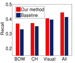
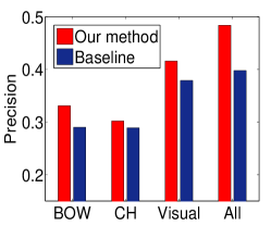
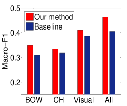
In this problem, we aim to predict high-level concepts from images. There are $81$ concepts in total but each image is typically assigned to $2$ concepts. This is cast as a multilabel prediction problem (Sec. 4.2.2). To create a baseline, we use a $k$-nearest neighbor classifier [37]. First we normalize multityped visual features as in Section 5.1. Then for the prediction, we retrieve top $30$ similar training images for each test image and estimate label probabilities. Labels that have higher probability than the estimated threshold will be selected. Whenever possible, we use tag ranking as an auxiliary task in addition to the main concept labeling task during training.

Figs. 3(a,b,c) plot the prediction results on the test set under three performance metrics: recall, precision and macro-F1. The results largely reflect the findings in the retrieval experiments: (i) multiviews work better than single view, (ii) tags are informative and thus should be exploited sensibly, (iii) the deep architecture outperforms shallow one. In particular, fusing all visual views leads to 21.8% (baseline) and 23.1% (deep) improvements in macro-F1 over the single view of color histogram. When tags are integrated as inputs, the improvement is higher: 39.0% using our deep architecture, and 27.8% for the baseline. Our macro-F1 is 12.6% better than the baseline on BOW alone and 14.3% better on the fusion of all types and modalities.

6 Conclusion

We have introduced a deep architecture and a learning procedure to discover joint homogeneous representation from multityped multimedia objects. We have also presented the concept of multityped tasks which deviate from the common single-type multitask setting. The deep learning procedure has two phases, the unsupervised and supervised. The unsupervised phase starts from the bottom layer, where type-specific features are modeled using separate RBMs, creating mid-level representations. All these representations are then aggregated into a second level RBM. In the supervised phase, the two layers are then fused into a deep neural network whose top layer is connected to one or more tasks of interest. The whole network is then discriminatively trained to obtain more predictive representation, starting from the parameters estimated in the unsupervised phase. In summary, our architecture seamlessly supports compact feature discovery from multimodal, multityped data under multityped multitask settings. Its capacity has been demonstrated on the tasks of image retrieval and multiple concept prediction showing promising results.

It should be emphasized that the proposed architecture is modular. Other types, more complex objects and tasks can be integrated easily. Word counts, for example, can be modeled by replicated softmax [21], an extension of the multinomial model (see also Eq. (13)). This paper is limited to a 3-layer deep architecture, but it can be extended straightforwardly with more layers in each step.

References

- [1] Rie Kubota Ando and Tong Zhang. A framework for learning predictive structures from multiple tasks and unlabeled data. The Journal of Machine Learning Research, 6:1817–1853, 2005.
- [2] Galen Andrew, Raman Arora, Jeff Bilmes, and Karen Livescu. Deep canonical correlation analysis. In Proceedings of the 30th International Conference on Machine Learning, pages 1247–1255, 2013.
- [3] Kobus Barnard, Pinar Duygulu, David Forsyth, Nando De Freitas, David M Blei, and Michael I Jordan. Matching words and pictures. The Journal of Machine Learning Research, 3:1107–1135, 2003.
- [4] Yoshua Bengio, Aaron Courville, and Pascal Vincent. Representation learning: A review and new perspectives. IEEE Transactions on Pattern Analysis and Machine Intelligence, 35(8):1798–1828, 2013.
- [5] R. Caruana. Multitask learning. Machine Learning, 28(1):41–75, 1997.
- [6] Weiwei Cheng, Eyke Hüllermeier, and Krzysztof J Dembczynski. Label ranking methods based on the Plackett-Luce model. In Proceedings of the 27th International Conference on Machine Learning (ICML-10), pages 215–222, 2010.
- [7] T.S. Chua, J. Tang, R. Hong, H. Li, Z. Luo, and Y. Zheng. NUS-WIDE: A real-world web image database from National University of Singapore. In Proceedings of the ACM International Conference on Image and Video Retrieval, page 48. ACM, 2009.
- [8] Paul Duchnowski, Uwe Meier, and Alex Waibel. See me, hear me: integrating automatic speech recognition and lip-reading. In ICSLP, volume 94, pages 547–550. Citeseer, 1994.
- [9] A. Elisseeff and J. Weston. A kernel method for multi-labelled classification. Advances in neural information processing systems, 14:681–687, 2001.
- [10] Dumitru Erhan, Yoshua Bengio, Aaron Courville, Pierre-Antoine Manzagol, Pascal Vincent, and Samy Bengio. Why does unsupervised pre-training help deep learning? The Journal of Machine Learning Research, 11:625–660, 2010.
- [11] Matthieu Guillaumin, Jakob Verbeek, and Cordelia Schmid. Multimodal semi-supervised learning for image classification. In Computer Vision and Pattern Recognition (CVPR), 2010 IEEE Conference on, pages 902–909. IEEE, 2010.
- [12] G.E. Hinton. Training products of experts by minimizing contrastive divergence. Neural Computation, 14:1771–1800, 2002.
- [13] G.E. Hinton and R.R. Salakhutdinov. Reducing the dimensionality of data with neural networks. Science, 313(5786):504–507, 2006.
- [14] K. Järvelin and J. Kekäläinen. Cumulated gain-based evaluation of IR techniques. ACM Transactions on Information Systems (TOIS), 20(4):446, 2002.
- [15] Yoonseop Kang, Saehoon Kim, and Seungjin Choi. Deep learning to hash with multiple representations. In ICDM, pages 930–935, 2012.
- [16] N. Le Roux, N. Heess, J. Shotton, and J. Winn. Learning a generative model of images by factoring appearance and shape. Neural Computation, 23(3):593–650, 2011.
- [17] J. Ngiam, A. Khosla, M. Kim, J. Nam, H. Lee, and A.Y. Ng. Multimodal deep learning. In ICML, 2011.
- [18] Bahadir Ozdemir and Larry S Davis. A probabilistic framework for multimodal retrieval using integrative indian buffet process. In Advances in Neural Information Processing Systems, pages 2384–2392, 2014.
- [19] Nikhil Rasiwasia, Jose Costa Pereira, Emanuele Coviello, Gabriel Doyle, Gert RG Lanckriet, Roger Levy, and Nuno Vasconcelos. A new approach to cross-modal multimedia retrieval. In Proceedings of the international conference on Multimedia, pages 251–260. ACM, 2010.
- [20] R. Salakhutdinov and G. Hinton. Deep Boltzmann Machines. In Proceedings of The Twelfth International Conference on Artificial Intelligence and Statistics (AISTATS’09, volume 5, pages 448–455, 2009.
- [21] R. Salakhutdinov and G. Hinton. Replicated softmax: an undirected topic model. Advances in Neural Information Processing Systems, 22, 2009.
- [22] R. Salakhutdinov and G. Hinton. Semantic hashing. International Journal of Approximate Reasoning, 50(7):969–978, 2009.
- [23] R. Salakhutdinov, A. Mnih, and G. Hinton. Restricted Boltzmann machines for collaborative filtering. In Proceedings of the 24th International Conference on Machine Learning (ICML), pages 791–798, 2007.
- [24] Arnold WM Smeulders, Marcel Worring, Simone Santini, Amarnath Gupta, and Ramesh Jain. Content-based image retrieval at the end of the early years. Pattern Analysis and Machine Intelligence, IEEE Transactions on, 22(12):1349–1380, 2000.
- [25] P. Smolensky. Information processing in dynamical systems: Foundations of harmony theory. Parallel distributed processing: Explorations in the microstructure of cognition, 1:194–281, 1986.
- [26] Nitish Srivastava and Ruslan Salakhutdinov. Multimodal learning with deep boltzmann machines. Journal of Machine Learning Research, 15:2949–2980, 2014.
- [27] T. Tran, D. Phung, and S. Venkatesh. Thurstonian Boltzmann Machines: Learning from Multiple Inequalities. In International Conference on Machine Learning (ICML), Atlanta, USA, June 16-21 2013.
- [28] T. Tran, D.Q. Phung, and S. Venkatesh. Mixed-variate restricted Boltzmann machines. In Proc. of 3rd Asian Conference on Machine Learning (ACML), Taoyuan, Taiwan, 2011.
- [29] T.T. Truyen, D.Q. Phung, and S. Venkatesh. Ordinal Boltzmann machines for collaborative filtering. In Twenty-Fifth Conference on Uncertainty in Artificial Intelligence (UAI), Montreal, Canada, June 2009.
- [30] Vladimir Vapnik and Akshay Vashist. A new learning paradigm: Learning using privileged information. Neural Networks, 22(5):544–557, 2009.
- [31] P. Vincent, H. Larochelle, I. Lajoie, Y. Bengio, and P.A. Manzagol. Stacked denoising autoencoders: Learning useful representations in a deep network with a local denoising criterion. The Journal of Machine Learning Research, pages 3371–3408, 2010.
- [32] M. Welling, M. Rosen-Zvi, and G. Hinton. Exponential family harmoniums with an application to information retrieval. In Advances in Neural Information Processing Systems, volume 17, pages 1481–1488. 2005.
- [33] Liang Xie, Peng Pan, Yansheng Lu, and Shixun Wang. A cross-modal multi-task learning framework for image annotation. In Proceedings of the 23rd ACM International Conference on Conference on Information and Knowledge Management, pages 431–440. ACM, 2014.
- [34] E. Xing, R. Yan, and A.G. Hauptmann. Mining associated text and images with dual-wing harmoniums. In Proceedings of the 21st UAI, 2005.
- [35] Ben P Yuhas, Moise H Goldstein Jr, and Terrence J Sejnowski. Integration of acoustic and visual speech signals using neural networks. Communications Magazine, IEEE, 27(11):65–71, 1989.
- [36] Daoqiang Zhang, Dinggang Shen, Alzheimer’s Disease Neuroimaging Initiative, et al. Multi-modal multi-task learning for joint prediction of multiple regression and classification variables in Alzheimer’s disease. Neuroimage, 59(2):895–907, 2012.
- [37] Min-Ling Zhang and Zhi-Hua Zhou. ML-KNN: A lazy learning approach to multi-label learning. Pattern recognition, 40(7):2038–2048, 2007.