The advantages of using a Lucky Imaging camera for observations of microlensing events

Abstract

In this work, we study the advantages of using a Lucky Imaging camera for the observations of potential planetary microlensing events. Our aim is to reduce the blending effect and enhance exoplanet signals in binary lensing systems composed of an exoplanet and the corresponding parent star. We simulate planetary microlensing light curves based on present microlensing surveys and follow-up telescopes where one of them is equipped with a Lucky imaging camera. This camera is used at the Danish $1.54$-m follow-up telescope. Using a specific observational strategy, For an Earth-mass planet in the resonance regime, where the detection probability in crowded-fields is smaller, lucky imaging observations improve the detection efficiency which reaches $2$ per cent. Given the difficulty of detecting the signal of an Earth-mass planet in crowded-field imaging even in the resonance regime with conventional cameras, we show that Lucky Imaging can substantially improve the detection efficiency.

1 Introduction

Gravitational microlensing refers to the bending of light by the gravitational potential of a stellar object Einstein (1936); Paczyński (1986). In this type of lensing, images from the source can not be resolved by a typical ground based telescope Chang & Refsdal (1979). Mao and Paczyński (1991) proposed using this phenomenon for detecting planets, where planet and parent star compose a binary system. This method has also been discussed earlier by Liebes in 1964. In this type of microlensing events, a planet produces anomalies in the light curve through the perturbation in the gravitational potential of the primary lens Gould & Loeb (1992). This perturbation can have weak and strong features on the light curve of a microlensing event, depending on the geometrical configuration of the source star with respect to the caustic lines in the lens plane. The observability of this anomaly is mostly sensitive to the planet distance to the parent star on the lens plane, so-called ’lensing zone’. This zone ranges in $[0.6,1.6]\mathrm{\theta_{E}}$ Gould & Loeb (1992); Bennett & Rhie (1996); Griest & Safizadeh (1998) where $\mathrm{\theta_{E}}$ is the angular Einstein radius and corresponds to the ring shape image when the observer, source and lens are completely aligned. Moreover, in close/wide high-magnification microlensing events when the source star crosses the caustic lines close to the lens or the companion planet, the planetary signals can be detected Shin et al. (2012).

The detectability of an exoplanet depends on the parameters of the lensing system. These parameters are (i) planet to the host star mass ratio, (ii) the angular separation, (iii) projected trajectory of the source star on the lens plane and (iv) the size of the source star. The advantage of planet detection by microlensing is that this method enables exploring planets of Earth mass or even lower mass planets Beaulieu et al. (2006); Muraki et al. (2011); Dominik et al. (2008); Paczyński (1996). While Earth-mass planets have also been detected by the Kepler space telescope and by the eclipsing method (e.g. Quintana et al. 2014), the advantage of using gravitational microlensing is to detect planets beyond the snow line of their parent stars and explore planets orbiting low-mass stars Sumi et al. (2010); Batista et al. (2011).

One of the problems in microlensing observations is the blending effect of the source star. This effect refers to the contribution of light from dense stellar fields within the Point Spread Function (PSF) of the source star towards the Galactic bulge. The result is imposing uncertainties on the calculation of the lens parameters. One of the approaches for decreasing the blending effect is using space-based telescopes for microlensing observations Bennett & Rhie (2002). The other low-costs method for improving the angular resolution of images from ground-based telescopes is using active adaptive optics or Lucky Imaging cameras.

The Lucky Imaging or Lucky exposure technique was first proposed in the 1960s to decrease the effect of atmospheric turbulence on astronomical images (e.g. Hufnagel & Stanley 1964). In this method, a series of images is taken with exposure times shorter than the time scale of the atmospheric turbulence. Then, the best images with flatter wavefront are selected, re-centered and combined to get a high resolution image. In order to quantify the quality of images, we can use the Strehl ratio Strehl (1895) which is the ratio of observed peak intensity to the theoretical peak intensity of a perfect image at the diffraction limit (Baldwin et. al. 2001). The first numerical calculation of Lucky Imaging in order to have a Lucky short-exposure image was done by Fried (1978). The next development was carried out by a group in Cambridge operating a Lucky Imaging camera on the Nordic Optical Telescope (NOT) with $2.56$ m aperture and obtained diffraction-limited images at wave lengths of $810$ nm Baldwin et al. (2001); Law et al. (2006). This group could improve the Strehl ratio in visible bands on a large telescope by combining this method with the adaptive optics method Law et al. (2009). They could make images with high resolutions from Mars and the other planets Dantowitz et al. (2000); Cecil & Rashkeev (2007).

We simulate the observing strategy with the Lucky Imaging camera used for follow-up microlensing observations at the Danish $1.54$-m telescope operated by the Microlensing Network for the Detection of Small Terrestrial Exoplanets (MINDSTEp) consortium . This telescope follows the observing strategy using a Lucky Imaging camera and EMCCDs (Dominik et al. 2010). We introduce an optimum method for analyzing light curves being observed both with Lucky Imaging and normal cameras. The main goals of this strategy are (i) decreasing the blending effect and enhancing signals from the anomalies on the light curve by selecting only the high-quality images and (ii) increasing the number of data points by considering all the photons gathered by the telescope(s) (providing high speed photometry enables us to correct instrumental effects and rebin and unrebin datasets). Finally, we investigate the improvement on the planet detection efficiency considering improvement of the blending effect with using the Lucky Imaging camera.

The outline of this paper is as follows: in section (2) we investigate the blending effect on the detectability of exoplanet microlensing events. In the next section, we review the Lucky Imaging technique and study the best observational strategy for detecting microlensing events via a Lucky Imaging camera. The effect of using a Lucky camera on the planetary detection efficiency will be discussed in section (4). Conclusions and summary are given in section (5).

2 The effect of Blending on the detectability of exoplanet microlensing signals

The blending effect on the planet detection efficiency as a function of the source radius was quantitatively investigated by Vermaak (2000). Also, Gaudi & Sackett (2000a) introduced an algorithm to calculate the planet detection efficiency for the observed microlensing light curves which contain the blending effect. They noticed that it is crucial the accurate determination of the blended light fraction for the accurate determination of the efficiency of individual events. In this part our aim is to show qualitatively the effect of blending on the planet signatures.

The intrinsic magnification of a source star is suppressed by including the blending of the background stars. These stars contribute inside the area of Point Spread Function (PSF) of the source star. Then the observed magnification $\mathrm{A_{obs}}$ as the ratio of the observable flux to the baseline flux is related to the intrinsic magnification of source star, $\mathrm{A_{\star}}$ by:

$$A_{obs}=(1-b)+bA_{\star},$$ (1)

where $b$ is the blending parameter which is the ratio of the source flux to the total baseline flux, without lensing effect:

$$b=\frac{F_{\star}}{F_{\star}+F_{bg}},$$ (2)

where $\mathrm{F_{\star}}$ is the intrinsic flux of the source star and $\mathrm{F_{bg}}$ is the baseline flux due to background stars within the source PSF. For the case of $\mathrm{b=1}$ there is no blending and $\mathrm{b=0}$ is the maximum blending. From the microlensing observations, determining the intrinsic source and baseline fluxes and as a result the blending parameter from light curves is difficult and there is uncertainty in this parameter. Hence, the blending effect can not always be removed from light curves. On the other hand the blending of source star by increase the level of background makes it hard to confirm the planetary signals.

Figure 1: Relative observed signal to the relative intrinsic signal, e.g. due to an exoplanet, in a microlensing light curve, i.e. equation (4), as a function of the intrinsic magnification of the source star $\mathrm{A_{\star}}$ and the blending parameter $b$.

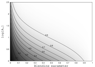
In order to quantify the effect of blending on an exoplanet signal in the light curve, let us assume the effect of companion planet in the binary lens is a perturbation on the Paczyński’s single lens light curve. Then, a perturbation $\mathrm{\delta A_{\star}}$ is related to the observed magnification $\mathrm{\delta A_{obs}}$, as follows

$$(\delta A/A)_{obs}=({\delta A}/{A})_{\star}\frac{A_{\star}}{A_{\star}+b^{-1}-1},$$ (3)

where we can call $\mathrm{\delta A/A}$ as the relative contrast and for two extreme limits of $\mathrm{b\rightarrow 0}$, we get no signal from the exoplanet and for the case that $\mathrm{b=1}$, we get the maximum signal.

Figure 2: The distribution of blending parameter towards the Galactic bulge for $3560$ OGLE-III microlensing events (Wyrzykowski et al. 2014).

We can define the relative observed signal to the intrinsic signal of source star by

$$Y=\frac{(\delta A/A)_{obs}}{({\delta A}/{A})_{\star}},$$ (4)

here the denominator of this expression (i.e. $\mathrm{({\delta A}/{A})_{\star}}$) depends on the parameters of the binary lens as the distance of the planet from the parent star, the mass ratio and relative position of the lenses and the source star as well as the angular size of the source star. On the other hand, the numerator (i.e. $\mathrm{({\delta A}/{A})_{obs}}$) depends on the signal to noise ratio of the observed data in the light curve.

Figure (1) represents the $\mathrm{Y}$ parameter as a function of the intrinsic magnification of the source star and the blending parameter. In order to get a strong signal from the planet either the magnification of the source star should be high enough or the blending parameter needs to be larger. The amount of blending depends on the luminosity of the source star and density of the field. The distribution of the blending parameter of microlensing events for $3560$ events, observed by the OGLE collaboration towards the Galactic bulge for the period of years 2001-2009 Wyrzykowski et al. (2014) is given in Figure (2).

In what follows, we investigate the blending effect on the detectability of an exoplanet signal in the flux. We perturb the source flux as a result of the presence of an exoplanet. The relative observed variation of flux relates to the relative intrinsic variation of flux as:

$$(\frac{\delta F}{F})_{obs}=b(\frac{\delta F}{F})_{\star}.$$ (5)

We can rewrite this equation in terms of magnitude as $\mathrm{\Delta m_{obs}=b\Delta m_{\star}}$. Having larger $b$ (e.g. with the Lucky Imaging method that will be discussed later), we can observe larger variations in the magnitude of the star. Let us assume the magnification of simple microlensing light curve is $\mathrm{A_{\star}}$ and any perturbation around it is $\mathrm{\delta A_{\star}}$. Then, the overall flux taking into account the background flux would be:

$$F_{obs}=F_{\star}(A_{\star}+\delta A_{\star})+F_{bg},$$ (6)

where using the definition of blending parameter which is brought in the equation (2):

$$F_{obs}=F_{\star}(A_{\star}+\delta A_{\star}+b^{-1}-1).$$ (7)

The photometric error bar, due to error in the source flux as well as other sources for the noises is given by

$$\delta F_{obs}=\frac{h\nu}{t_{exp}}\sqrt{\frac{t_{exp}}{h\nu}F_{\star}(A_{\star}+\delta A_{\star}+b^{-1}-1)+C(t)^{2}},$$ (8)

where $\mathrm{\nu}$ is the frequency of the light, $\mathrm{t_{exp}}$ is the exposure time and $C$ represents other noise terms excluding noise in the source flux (e.g. readout noise, dark noise, constant gain, extra noise from fast readouts for the Lucky Imaging camera, etc). We note that $C$ generally depends on time. This is because the blending effect in microlensing events is usually estimated via difference imaging and is therefore affected by the choice of reference frame. The reference frames for different observational groups are chosen at different times. Since the baseline flux changes with time, so changes $\mathrm{C}$ representing other noise terms except for the time-dependent uncertainty in source flux. However, the photometric error depends on the number of pixels which is not considered here.

The observability of a signal means that a perturbation in the observed flux, $\mathrm{\Delta F}$, would be at least larger than the photometric error bar, i.e. $\mathrm{\Delta F>\delta F_{obs}}$. According to the amount of the perturbation in the observed flux as $\mathrm{\Delta F=F_{\star}\delta A_{\star}}$, the observability condition results in:

$$N_{p}>\frac{1}{\delta A_{\star}^{2}}\left[A_{\star}+\delta A_{\star}+b^{-1}-1+\frac{C(t)^{2}h\nu}{F_{\star}t_{exp}}\right],$$ (9)

where $\mathrm{N_{p}=F_{\star}t_{exp}/(h\nu)}$ represents the number of photons from the source star for a given exposure time. Having smaller $b$ requires a larger number of photons. In the next section, we will discuss the possibility of decreasing the blending effect using the Lucky Imaging camera.

Figure 3: Lucky Imaging of an averaged PSF by the Danish telescope. The left panel shows a diffraction-limited stellar PSF extracted from the Lucky Imaging camera obtained from the DANDIA pipeline (Bramich 2008). The right panel represents the same image taken by the Danish Faint Object Spectrograph and Camera (DFOSC). The image scales are $0.09\mathrm{~{}arcsec/pixel}$ for the Lucky Imaging camera and $0.39\mathrm{~{}arcsec/pixel}$ for DFOSC.

3 Observations of planetary microlensing events with a Lucky Imaging camera

In this section we investigate the characteristics of the Lucky Imaging method and introduce a strategy for the observation of planetary microlensing events with the Lucky Imaging camera. We assume that the Lucky Imaging observation is carried out by the Danish telescope which is one of the follow-up telescopes.

3.1 The Lucky Imaging method

One of the challenging problems of photometry and imaging in astronomy is dealing with atmospheric seeing variations. The seeing parameter increases with atmospheric turbulence where the wave front of a distance source gets distorted by crossing different layers of the atmosphere. Usually a telescope receives distorted wave fronts; but occasionally we can find flat wave fronts. The probability of finding such a wave front depends on the size of the wave front patch arriving at the primary mirror of the telescope. Hence, we expect that smaller telescopes are more likely to receive flat wave fronts compared to larger telescopes in optical wavelengths. The probability of a diffraction-limited image detected by a telescope with an aperture size of $D$ in an instant of time while the wave front crosses the atmospheric turbulence is given by Fried (1978):

$$P\simeq 5.6\exp{(-0.1557\times{D^{2}/r_{0}^{2}})},$$ (10)

where $\mathrm{r_{0}}$ is the coherent length which is defined as the diameter of an area over which the root mean square (rms) of phase variation due to the atmospheric turbulence is equal to $1$ radian Fried (1978). This parameter defines the seeing of observation equal to $\mathrm{\sim 251\lambda/r_{0}}$ where $\mathrm{\lambda}$ is the wave length in $\mu$m, $\mathrm{r_{0}}$ is in mm and seeing is given in the unit of the arc second. At wave length of $\sim 500$ nm, the most common value of $\mathrm{r_{0}}$ is about $10-15$ cm, but in good conditions the value of this parameter reaches to $30-40$ cm. So the least amount of $\mathrm{D/r_{0}}$ for $1$-meter class telescopes in visible band is about $\sim 3$. We can interpret $\mathrm{D/r_{0}}$ as the ratio of ”seeing” to ”diffraction limit” of a telescope:

$$\frac{\theta_{seeing}}{\theta_{diff}}=\frac{D}{r_{0}},$$ (11)

where minimum discernable angular separation of two sources by considering diffraction limit is equal to $\mathrm{\theta_{diff}(rad)=1.22\lambda(cm)/D(cm)}$. The probability function for taking a Lucky short exposure image from equation (10) is a decreasing function versus $\mathrm{D/r_{0}}$ where $\mathrm{D/r_{0}}$ usually ranges between $\mathrm{4<D/r_{0}<7}$ Hecquent & Coupinot (1985).

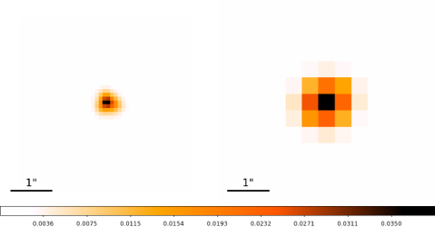
In Lucky Imaging, we select a fraction of images to construct a final image with a smaller Full Width at Half Maximum (FWHM) value or in other words larger Strehl ratio Law et al. (2009). However, just by re-centering all taken images with the Lucky camera, we can already decrease the FWHM (see Figure (4) of Law et al.2006). A decrease in FWHM in a given seeing amount is quantified by the so-called improvement factor (IF), defined as:

$$IF=\frac{FWHM_{\star}}{FWHM_{lc}},$$ (12)

where $\mathrm{FWHM_{\star}}$ is the mean of FWHM of a typical source star observed by a telescope without using the Lucky Imaging camera for a given amount of seeing and $\mathrm{FWHM_{lc}}$ is the FWHM of the final image produced by a Lucky Imaging camera Law et al. (2006). Hence, using Lucky Imaging the stellar PSF decreases and can even reach the diffraction limit. Figure (3) illustrates this point: the left panel represents a diffraction-limited stellar PSF extracted from the Lucky Imaging camera at the Danish $1.54$-m telescope (EMCCD) obtained from the DANDIA pipeline Bramich (2008). The right panel shows the same image taken by the Danish Faint Object Spectrograph and Camera (DFOSC). The image scales are $\mathrm{0.09~{}arcsec/pixel}$ for the Lucky Imaging camera and $\mathrm{0.39~{}arcsec/pixel}$ for DFOSC. The PSF area for the image taken by Lucky Imaging (left panel) is about $\mathrm{0.2~{}arcsec^{2}}$ and that for the image taken by DFOSC (right panel) is $\mathrm{1.1~{}arcsec^{2}}$, where we define the PSF area by $\Omega=\pi(FWHM/2)^{2}$. Consequently, this method reduces the PSF area and blending by the background stars. By selecting only the best images, the final image will have a smaller PSF area or higher IF.

Figure 4: Left panel: the number of blended stars whose lights enter the PSF of source star (red solid line) and blending parameter (black dotted line) as a function of IF. Right panel: variation of apparent magnitude of the stellar PSF versus IF (red solid line) and percentage of the selected frames (black dotted line). Here, we take the angular distribution of stars in the Galactic bulge from the synthetic Besançon model (Robin et al. 2003) and set the apparent magnitude of the source star is $\mathrm{m_{\star}=20.0}$ mag, the initial amount of the blending parameter is $\mathrm{b=0.13}$ and $\mathrm{seeing}=0.9~{}\mathrm{arcsec}$.

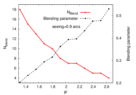
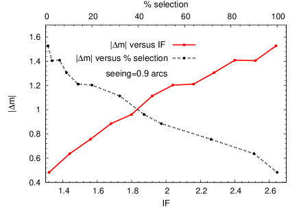
In order to find an optimum procedure of observation with the Lucky Imaging method, we consider a highly-blended area of stars in the Galactic bulge and determine the blending parameter as follows. First we calculate the average number of blended stars by integrating over the number density of the Galactic bulge stars along the the line of sight and the boundary of integral within the area of the source PSF, i.e. $\mathrm{<N_{blend}>=\int\rho(D,\Omega_{\star})D^{2}dD\Omega}$, where $\mathrm{D}$ is the distance from the observer position, $\mathrm{\Omega_{\star}}$ is the angular position of the source star. We take the number density of the Galactic bulge, $\mathrm{\rho}$, from the Besançon model Dwek et al. (1995); Robin et al. (2003). For these stars, we have the absolute magnitude according to their mass, age and metallicity. Then, the apparent magnitude of each blended star is calculated according to the absolute magnitude, distance modulus and extinction. The extinction map towards the Galactic bulge as a function of distance is adapted from Gonzalez et al. (2012).

Figure (4) shows the number of background stars which contribute in the PSF of source star (red solid line) and the blending parameter (black dotted line) versus IF. We note that increasing IF decreases the PSF area of the source star for a given amount of seeing. Also we show (in the left panel) the variation of the apparent magnitude in that stellar PSF versus IF (red solid line) and fraction of selected frames (black dotted line). Here, we use the relation between percentage of selected frames and IF for the fixed seeing amount (i.e. $\mathrm{0.9~{}arcsec}$) given by Law et al. (2006). However, according to the Fried(1978)’s relation the probability of getting a diffraction-limited image by the Danish telescope at $\mathrm{R}$ band is even a little higher than that by NOT at $\mathrm{I}$ band, if it would not be optics-limited. Decreasing the PSF area with the Lucky Imaging method deblends the apparent magnitude of the stellar PSF due to decreasing the number of blended stars. In these figures, we set the apparent magnitude of the source star to $\mathrm{m_{\star}=20.0}$ mag, the initial amount of the blending is $\mathrm{b=0.13}$ and $\mathrm{seeing=0.9~{}\mathrm{arcsec}}$. Noting that in reality seeing is changing with time during the observation. Hence, we choose the different fractions of images in different seeing amounts to have constant PSF area throughout the observation.

Figure 5: Seeing variation versus time (red solid line) for every $20$ min and the corresponding percentage of selected frames (black dashed line) to get a constant PSF area of the source star, $\mathrm{{\Omega}=0.27~{}arcsec^{2}}$.

Lucky imaging observations reduce the blending and the PSF size by selecting high quality images and the aim to (i) better constrain the blending parameter, (ii) make a more reliable fit of the parameters of the microlensing light curves and (iii) detect small perturbations in the light curve, such as planetary signals (see equation 3).

3.2 An observational strategy for using a LI camera

In what follows, we introduce a strategy for analyzing microlensing light curves hypothetically being observed both by the Lucky Imaging and normal cameras. Our aim is to optimize the quality of the light curves, by means of having less blending of the source star, enough cadence in the light curve and the least photometric uncertainties for data points. In the simulation we keep the two crucial parameters constant throughout the light; (i) we select the frames from the Lucky imaging camera in such a way that the source PSF area is a constant parameter and (ii) for each data point, we stack enough images from the lucky camera to have constant photometric accuracy throughout the light curve.

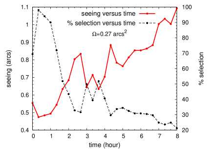
We note that in reality during the observation, the ”seeing” parameter changes with time and in order to have a constant PSF area of the source star, we should have a time dependent procedure for choosing percentage of the selected frames from each spool of images. An example that demonstrate the variation of seeing versus time is shown in Figure (5). Here, the seeing parameter (red solid line) is shown with the cadence of $20$ minutes. In our simulation, the seeing amounts are chosen from a synthetic series of seeing data points which were archived by the La Silla observatory

Keeping a constant value for the PSF area of the source star (e.g. $\mathrm{\Omega=0.27~{}arcsec^{2}}$), we calculate the percentage of the selected frames corresponding to each value of seeing. Following this strategy, during the microlensing event, blending parameter which is specified by the PSF area of source star is set to be a constant value. On the other hand, adapting the second condition, we use an enough number of images to get a threshold value for the photometric precision. This factor can be tuned by the effective exposure time for each data point ($\mathrm{t_{exp}}$) to have uniform error bars throughout the light curve, as suggested in Dominik et al.$(2010)$. Since the magnification factor for each data point is different, the signal to noise ratio is different at each moment. According to the definition, the photometric accuracy is given by:

$$\frac{\sigma_{F}}{F}=\frac{\sigma_{N_{p}}}{N_{p}},$$ (13)

where $N_{p}$ is the total number of photons collected in PSF of the source star and $\mathrm{\sigma_{N_{p}}=\sqrt{N_{p}}}$ is the photon-count noise. To get uniform error bars for data points the signal to noise ratio for each data point should reach to a threshold amount where signal is defined as the total number of photons:

$$N_{p} = [(A_{\star}-1)10^{-0.4m_{\star}}+\Omega 10^{-0.4\mu_{sky}}$$ (14)

$$+ \sum_{i=1}^{N_{blend}}10^{-0.4m_{i}}]10^{0.4m_{zp}}\times t_{exp},$$

where $\mathrm{A_{\star}}$ is the magnification factor of the source star, $\mathrm{m_{\star}}$ is the apparent magnitude of source star, $\mathrm{m_{i}}$ is the apparent magnitude of $i$th background star within the PSF of source star, $\mathrm{N_{blend}}$ is the total number of blended stars, $\mathrm{\mu_{sky}}$ is sky brightness in $\mathrm{mag/arcsec^{2}}$ unit and $\mathrm{m_{zp}}$ is the zero point magnitude which is equivalent to a photon collected over the unit of the area of the telescope per unit of time. According to the definition of magnitude, $\mathrm{m_{v}^{zp}}$ is given by:

$$m_{v}^{zp}=-2.5\log(\frac{h\nu}{\pi(D/2)^{2}F_{0}}),$$ (15)

where $\mathrm{F_{0}}$ is the absolute flux corresponding to the magnitude of zero. Bessell (1979). We keep the signal to noise ratio of $500$ for lucky imaging data points throughout the light curve. Note that the total observing time in terms of the effective exposure time will be: $\mathrm{T_{obs}=t_{exp}/f}$, where $\mathrm{f}$ is the fraction of selected frames. We note that $\mathrm{T_{obs}}$ is longer than $t_{exp}$.

Figure 6: A simulated planetary microlensing light curve. Its theoretical light curve is shown with green dashed line. The simulated data points over this light curve hypothetically taken by the Danish telescope and other (survey and follow-up) telescopes are represented by black stars and red circles respectively. The parameters used to make this light curve are $\mathrm{u_{0}=-0.04}$, $\mathrm{t_{E}=12days}$, $\mathrm{t_{0}=0}$, $\mathrm{\rho_{\star}=0.003}$, $\mathrm{q=3e-5}$, $\mathrm{d(R_{E})=0.9}$, $\mathrm{\theta=25^{\circ}}$, $\mathrm{m_{\star}=20.2~{}mag}$ and $\mathrm{b=0.13}$.

In reality a Lucky Imaging camera needs extra exposure times due to (i) the extra noise at the electron multiplication stage (the cascade can trigger unwanted extra electrons), (ii) extra noise by distributing the flux over many more pixels in case of not so optimal seeing or the worst seeing bins and (iii) extra noise due to the shift-and-add. The latter aspects are somewhat related, since the signal to noise ratio generally depends on the number of pixels used. The more we shift images, the more the different uncertainties in pixel-to-pixel sensitivity i.e. in the flatfield, sky, etc. All these aspects need more exposure times. The signal to noise ratio for the Lucky imaging camera is lower by a factor of $\mathrm{\sqrt{2}}$ as compared to regular CCDs Skottfelt et al. (2015). This penalty can be avoided if the EMCCD is operated in photon counting mode.

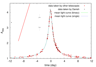
Here, we simulate the planetary microlensing light curve shown in Figure (6), being observed by a group of telescopes where one of them is the Danish $1.54$-m telescope. The parameters used to generate this light curve are $\mathrm{u_{0}=-0.04}$, $\mathrm{t_{E}=12~{}days}$, $\mathrm{t_{0}=0}$, $\mathrm{\rho_{\star}=0.003}$, $\mathrm{q=3\times 10^{-5}}$, $\mathrm{d(R_{E})=0.9}$, $\mathrm{\theta=25^{\circ}}$, $\mathrm{m_{\star}=20.2~{}mag}$ and $\mathrm{b=0.13}$ where $\mathrm{\theta}$ is the angle between the projected source trajectory and the binary axis and $\mathrm{\rho_{\star}}$ is the projected source radius normalized to the Einstein radius.

To produce synthetic data points over this light curve, we assume this light curve is being observed by survey and follow-up telescopes while follow-up observations are started after the magnification factor reaches to a given threshold (e.g. $\mathrm{\frac{3}{\sqrt{5}}}$). In order to make a realistic light curve in the simulation, cadences between the data points and the photometric uncertainties are taken from the archived microlensing model light curves along with data collected by the Optical Gravitational Lensing Experiment (OGLE), Microlensing Observations in Astrophysics (MOA), MiNDSTEp, follow-up observations of microlensing events with a robotic network of telescopes (ROBONet-II), Microlensing Follow-Up Network (MicroFUN) and Probing Lensing Anomalies Network (PLANET) . We adapt $20$ archived microlensing events and obtain the sampling time between consecutive data points from the observed data over the light curves as well as the photometric accuracy of data points.

We separate the simulated data points into two categories of being $\mathrm{A_{obs}\leq 3/\sqrt{5}}$ where only the survey telescopes with the cadence and photometry error of data associated with the surveys are chosen and $\mathrm{A_{obs}\geq 3/\sqrt{5}}$ after alerting the event where the specification of the surveys and follow-up telescopes are adapted. In order to make lucky imaging observation with the Danish telescope we label archived data points in reality taken by this telescope which is illustrated by black stars in Figure (6). Here we use the adaptive contouring method to calculate the magnification of the source star in the binary lensing Dominik (2007). The simulated data points are shifted with respect to the mean light curve according to their photometric uncertainties by a Gaussian function.

Figure (6) as a sample represents the data points over the simulated light curve. The data points by the Danish $1.54$-m telescope are in black stars and other surveys and follow-up telescopes are in red points. The inset represents the caustic curves (black solid curves) and the source trajectory with respect to the lens position projected on the lens plane (red solid line). Also the microlensing light curve with the planetary lens and simple Paczyński microlensing light curve are shown by green dashed and blue dotted lines, respectively.

In the next step, we regenerate this light curve by replacing data from the conventional camera in the Danish telescope with data taken by the Lucky camera. For simulating these data, the important quantity is the time interval between two consecutive data points. Since the Danish telescope simultaneously observes several microlensing targets during each night, so there is a time interval i.e. cadence, between data points of each light curve. There is an experimental relation between cadence $\mathrm{\tau}$ and the observed magnification factor Dominik et al. (2010):

$$\tau=90\sqrt{\frac{3/\sqrt{5}}{A_{obs}}}~{}~{}\rm{min}.$$ (16)

The crucial point regarding the sampling interval is that we set it to $\mathrm{\sim 10}$ minutes once at least three data points deviate from the simple microlensing light curve by more than $\mathrm{2\sigma}$. Once the anomaly is covered, we return to the normal sampling rate. In addition to the above cadence, we should consider the overhead time in between such as slew time and operational losses Dominik et al. (2010). The operational loss could be due to the weather, technical and operational issues. The average values of the overhead time in between two consecutive data points and the lost time for each data point taken by the Danish telescope are $\mathrm{\sim 1.57}$ min and $\mathrm{\sim 1.45}$ min, respectively. Considering Poisson uncertainties for these time scales, they are added to these two time scales.

Figure 7: Each panel shows the simulated microlensing light curve shown in Figure (6) which is modified by replacing data from the conventional camera on the Danish telescope with synthetic data hypothetically taken by Lucky Imaging (black stars), the rest of data points hypothetically taken by usual cameras (red circles). The light curves are plotted for four different values of $\mathrm{\Omega}$.

Figure 8: Data points hypothetically taken by normal cameras (red circles) in light curves of Figure (7) are shifted to the lower blending data points taken by Lucky Imaging. This shifting is done for various $\mathrm{\Omega}$s using $\mathrm{\alpha}$ parameters.

Figure 9: Imposing the factors $\mathrm{\kappa}$, all data points in light curves shown in Figure (8) are shifted to the least amount of blending effect corresponding to the least amount of $\mathrm{\Omega}$ (i.e. $\mathrm{\Omega=0.15~{}arcsec^{2}}$). Therefore, all of these light curves have the same (and the least) blending effects.

The Danish telescope monitors the Galactic bulge for $\mathrm{\sim 6.5}$ hours on average each night during the observing season. Also this telescope observes ongoing events during the night with a probability of $\mathrm{\sim 83}$ per cent Dominik et al. (2010) (i.e. no-observation might be due to weather condition, technical failure and etc). We consider all of these observational limitations in calculating cadences. To generate observational data points, the magnification factors are shifted according to a Gaussian function with the width of uncertainty in the magnification factor $\delta_{A}$. This uncertainty is calculated according to the noise $\mathrm{\sigma_{F}}$ and fractional systematic uncertainty for the Danish telescope $\mathrm{\sigma_{s}/F_{obs}=0.3\%}$ Dominik et al. (2010). The overall amount of uncertainly is given by $\delta_{A}=\sqrt{\sigma_{F}^{2}+\sigma_{s}^{2}}/F_{bg}$.

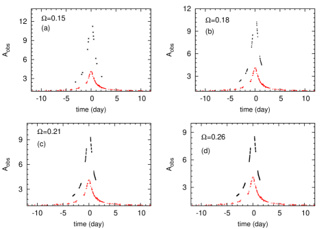
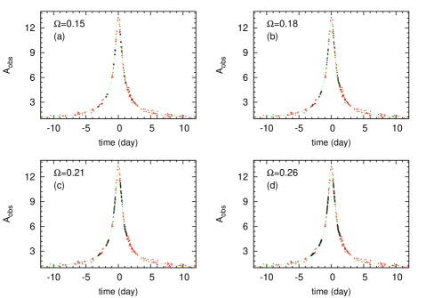
We consider different amounts of PSF area for the source star and for each case we simulate the observations with the Lucky Imaging camera on the Danish telescope. Figure (7) shows a sample of light curves with four different $\mathrm{\Omega}$s which depend on the images we select from the lucky camera data. Here the simulated data points hypothetically taken by the Lucky Imaging camera on the Danish telescope are shown by black signs and data points taken by other telescopes are shown with red circles. The crucial role of the Lucky Imaging camera is to enhance small perturbations in the light curve compare to the normal camera by decreasing the blending effect.

Let us divide data in the light curve into two sets of being observed by the Lucky camera with the Danish telescope and observed by the normal cameras with the other telescopes. Then, in order to fit the light curves with the theoretical model, we have different blending parameters for each data set:

$$A_{o}(t_{j}) = b_{o}A_{\star}(t_{j})+(1-b_{o})$$ (17)

$$A_{lc}(t_{j}) = b_{lc}A_{\star}(t_{j})+(1-b_{lc}),$$ (18)

where $\mathrm{A_{\star}}$ is the magnification factor of the source without considering blending effect, $\mathrm{A_{o}}$ is the observed magnification factor with normal cameras and $\mathrm{b_{o}}$ is the corresponding blending parameter. For the Lucky camera, $\mathrm{A_{lc}}$ is the observed magnification and $\mathrm{b_{lc}}$ is the corresponding blending parameter. Having less blending for the Lucky camera, means $\mathrm{b_{lc}}$ is larger than $\mathrm{b_{o}}$. After fitting theoretical light curves in equation (17) and (18) to the two sets of data points, we calculate the ratio of larger blending parameter to the smaller blending parameter, using the magnification factor from each light curve

$$\alpha=\frac{A_{lc}(t_{j})-1}{A_{o}(t_{j})-1}=\frac{b_{lc}}{b_{o}}.$$ (19)

Hence by imposing this factor, we can normalize the microlensing data points by shifting low quality blending data points to the high quality data points with the following transformation function:

$$A^{\prime}_{o}(t)=\alpha(A_{o}(t)-1)+1,$$ (20)

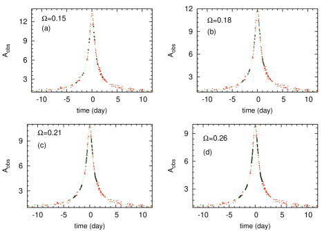
where $\mathrm{A^{\prime}_{o}}$ is the new value of data points taken by normal cameras. Figure (8) shows this shifting for different values of $\mathrm{\Omega}$s.

	$\mathrm{\Omega(arcsec^{2})}$	$\mathrm{\bar{f}[\%]}$	$\mathrm{\alpha_{n}\pm\Delta\alpha_{n}}$	$\mathrm{\bar{t}_{exp}(s)}$	$\mathrm{\bar{T}_{obs}(min)}$	$\mathrm{N}$
	$0.15$	1.7	3.9$\pm$0.073	203.2	45.4	206
	$0.18$	5.0	3.5$\pm$0.069	163.4	44.9	236
	$0.21$	12.0	3.2$\pm$0.061	162.4	21.0	291
	$0.26$	23.9	2.9$\pm$0.056	159.8	10.1	404
	$0.32$	43.0	2.4$\pm$0.049	155.3	5.6	579
	$0.40$	61.9	2.1$\pm$0.041	147.6	3.6	788
	$0.52$	93.4	1.8$\pm$0.036	144.3	2.5	1072

Table 1: This table represents some properties of different light curves corresponding to different amounts of the PSF area $\mathrm{\Omega}$ whose amounts are brought in the first column. The second and third columns show the average values of the percentage of the selected images throughout the light curves $\mathrm{\bar{f}[\%]}$ and $\mathrm{\alpha_{n}\pm\Delta\alpha_{n}}$ corresponding to each light curve respectively. Two next columns represent the averaged amounts of the effective exposure time for data points hypothetically taken by Lucky Imaging $\mathrm{\bar{t}_{exp}(s)}$ and the total observational time $\mathrm{\bar{T}_{obs}(min)}$. $\mathrm{N}$ represents the number of data points over each light curve.

Shifting data points with the factor of $\alpha$, imposes uncertainties in the data points due to the uncertainty in $\mathrm{\alpha}$. Relative error in $\mathrm{\alpha}$ due to errors in the blending parameters of each set of data points is given by:

$$(\frac{\Delta\alpha}{\alpha})^{2}=(\frac{\Delta b_{lc}}{b_{lc}})^{2}+(\frac{\Delta b_{o}}{b_{o}})^{2},$$ (21)

where $\mathrm{\Delta b_{lc}}$ and $\mathrm{\Delta b_{o}}$ are the uncertainties in the blending parameters which can be obtained from the maximum likelihood function of the best fit to the observed data. The optimum amounts of blending parameters for the minimum value of $\mathrm{\chi^{2}}$ obtains from $\mathrm{\partial\chi^{2}/\partial b=0}$, results in

$$b_{j}=\sum_{i}\frac{(A_{\star,i}-1)(A_{j,i}-1)}{\sigma^{2}}/\sum_{i}\frac{(A_{\star,i}-1)^{2}}{\sigma^{2}},$$ (22)

where $\mathrm{A_{j,i}}$ with $\mathrm{j=lc,o}$ is the observed value for the magnification and $\mathrm{A_{\star,i}}$ is intrinsic value of the magnification factor at the $i$the time from the best fit to the light curve. $\mathrm{\sigma}$ is the observational photometric precision.

Figure 10: Result from a Monte-Carlo simulation for the average value of $\mathrm{\Delta\alpha}$ (red solid line) and the blending parameter (black dotted line) versus the PSF area $\mathrm{\Omega}$.

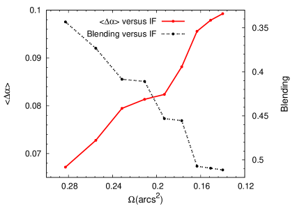
Therefore, according to the uncertainty of $\mathrm{b}$ we can obtain corresponding error of $\mathrm{\alpha}$ from equation (21). Figure (10) shows the relation between the error in $\mathrm{\alpha}$ and blending in terms of the PSF area for an ensemble of events. While decreasing $\mathrm{\Omega}$ improves the blending around the source star, it increases uncertainty in the $\mathrm{\alpha}$ due to lack of enough data points in the light curve. This effect also is shown in Table (1). Finally, the error bar corresponds to the magnification of the shifted data due to the error in $\mathrm{\alpha}$ and error in the initial magnification can be obtained from:

$$(\frac{\Delta A^{\prime}_{o}}{A^{\prime}_{o}})^{2}=(\frac{\Delta\alpha}{\alpha})^{2}+(\frac{\Delta A_{o}}{A_{o}-1})^{2}.$$ (23)

Accordingly, the error bars of data points set at the baseline of the microlensing light curves (i.e. $\mathrm{A_{o}\sim 1}$) increase significantly. Hence, the efficiency for detecting planetary signals located around the baseline of the high-blended microlensing light curves is not likely improved by the Lucky Imaging camera. These planetary signals mostly happen while crossing the planetary caustic curves close to the companion planets.

In Figure (8), it is seen that the normalization of the normal camera data points depends on PSF size that we adapted in the lucky imaging observation. The smaller PSF, results in a higher magnification factor. We may normalized all data points with moderate PSF values to the smallest PSF that is generated only by the best images from the lucky camera. This procedure results in maximizing the data points in the light curve. Let us define the best normalization factor with the best PSF value by $\alpha_{max}$, then the shift factor between light curves with different PSFs (i.e. $\alpha$s) can be defined as $\mathrm{\kappa={\alpha_{max}}/{\alpha}}$. Figure (9) shows the shifted light curves with different $\mathrm{\Omega}$s and $\mathrm{\alpha}$s with respect to the light curve with the smallest $\mathrm{\Omega}$ (i.e. ${\mathrm{0.15~{}arcsec}}$). We note that after shifting the data points, all light curves have normalized with the same factor.

	$\mathrm{\Omega(arcsec^{2})}$	$u_{0}$	$t_{E}(day)$	$\theta^{\circ}$	$b$	$d(R_{E})$	$q(\times 10^{-5})$	$n$	$\chi^{2}$	$\Delta\chi^{2}$	$\Delta\chi^{2}/n$
	$0.15$	-0.04	12.0	25.0	0.51	0.9	2.0	2	71.1	0.5	0.25
		-0.04	12.0	25.0	0.51				70.6
	$0.18$	-0.04	12.0	27.0	0.51	0.9	3.0	9	67.5	5.2	0.58
		-0.04	12.0	29.0	0.51				72.7
	$0.21$	-0.04	12.0	25.0	0.51	0.9	3.0	19	69.7	13.5	0.71
		-0.04	12.0	29.0	0.51				83.2
	$\mathrm{0.26(LB)}$	-0.04	12.0	25.0	0.51	0.9	3.0	38	70.1	32.6	0.86
		-0.04	12.0	29.0	0.51				102.7
	$0.32$	-0.04	12.0	25.0	0.51	0.9	3.0	71	84.3	45.4	0.64
		-0.04	12.0	29.0	0.51				129.7
	$0.40$	-0.04	12.0	25.0	0.51	0.9	3.0	109	96.8	72.3	0.66
		-0.04	12.0	29.0	0.51				169.1
	$0.52$	-0.04	12.0	25.0	0.51	0.9	3.0	171	110.7	109.2	0.64
		-0.04	12.0	29.0	0.51				219.9
	$\mathrm{1.02(LA)}$	-0.04	12.0	29.0	0.13	0.8	3.0	1	209.3	0.6	0.6
		-0.04	12.0	27.0	0.13				209.9

Table 2: This table shows the improvement in detectability of the planetary signal using our strategy. The first column indicates the amount of PSF area $(\Omega)$, corresponding to different light curves some of them are represented in different panels of Figures (7), (8) and (9). The light curve with $\mathrm{\Omega=1.02~{}arcsec^{2}}$ is shown in Figure (6) in which we do not use any Lucky Imaging camera. The next columns represent the best-fitted parameters from fitting different planetary microlensing events to the mentioned light curves. The theoretical parameters for making these light curves are $\mathrm{u_{0}=-0.04}$, $\mathrm{t_{E}=12days}$, $\mathrm{\rho_{\star}=0.003}$, $\mathrm{\theta=25^{\circ}}$, $\mathrm{t_{0}=0}$, $\mathrm{q=3\times 10^{-5}}$ and $\mathrm{d(R_{E})=0.9}$. We fixed $\mathrm{\rho_{\star}}$ and $\mathrm{t_{0}}$ to their true values in the fitting process. We note that the best fitted parameters as well as the minimum amounts of $\chi^{2}$ from fitting simple Paczyński microlensing models to different light curves are brought in the bottom rows corresponding to each light curve. $\mathrm{n}$ represents the number of data points hypothetically taken by Lucky Imaging and cover the planetary signal, i.e. located at the time interval of $\mathrm{[0.9:1.25]~{}days}$. Two next columns show the minimum value of $\mathrm{\chi^{2}}$ from fitting planetary (and simple Paczyński) microlensing events to the light curves as well as their differences. The last column represents the normalized amounts of $\Delta\chi^{2}$ to $\mathrm{n}$. The maximum amount of $\mathrm{\Delta\chi^{2}/n}$ occurs for the light curve with $\mathrm{\Omega=0.26~{}arcsec^{2}}$ and after shifting data points i. e. $\mathrm{LB}$.

Figure 11: This figure summarizes the issues of this subsection and shows that (i) the blending effect decreases the detectability of planetary signal in the microlensing light curve and (ii) the Lucky Imaging camera improves detectability of this signal by decreasing the blending effect. The red solid line represents the sample planetary microlensing event, studied in this subsection, without blending effect. The gray dashed lines show the best-fitted simple Paczyński microlensing light curves with different blending parameters. The blue dotted line shows that event with the blending effect, $\mathrm{b=0.13}$. The simulated data points with the corresponding error bars over this light curve are shown with the black stars (taken by the Danish telescope) and the red circles (taken by other telescopes hypothetically). This light curve is also shown in Figure (6), so-called LA. The green dashed line and its data points represents that light curve resulted from this assumption that the Danish telescope uses the Lucky Imaging camera for detecting it, so-called LB. In this light curve the blending effect improves up to the amount of $\mathrm{b=0.51}$, the error bars of data points increase due to the shifting process while the planetary signal becomes more detectable. The planetary signals of these light curves are enlarged in the inset of the figure.

We summarize the properties of the generated light curves corresponding to different amounts of the PSF area in the table (1). In this table, the second and third columns show the average values of the percentage of the selected images throughout the light curves $\mathrm{\bar{f}[\%]}$ and $\mathrm{\alpha_{n}\pm\Delta\alpha_{n}}$ corresponding to each light curve respectively. Two next columns represent the averaged amounts of the effective exposure time for data hypothetically taken by Lucky Imaging $\mathrm{\bar{t}_{exp}(s)}$ and the total observational time $\mathrm{\bar{T}_{obs}(min)}$. $\mathrm{N}$ represents the number of data points over each light curve. Noting that the effective exposure time depends on the PSF area and decreases by increasing it. Because we fix the photometric error bars throughout the light curves. The total observational time depends on the fraction of the selected images and increases by decreasing this factor.

In this part we examine the best value for the PSF size that we can choose from the lucky imaging observation. Our criterion is to maximize the signal to noise ratio of the planetary signal in the binary lensing with minimizing the $\mathrm{\chi^{2}}$ value from fitting to the model. We subtract $\mathrm{\chi^{2}}$ from the binary lensing and simple Paczyński microlensing (i.e. $\mathrm{\Delta\chi^{2}=\chi_{0}^{2}-\chi_{pl}^{2}}$) where large $\mathrm{\Delta\chi^{2}}$ indicates a better signal from the lensing. Table (2) shows the best-fitted parameters from fitting different planetary microlensing events as well as $\mathrm{\Delta\chi^{2}}$ in terms of various values of $\mathrm{\Omega}$ which corresponds to different light curves. This table shows that using a Lucky Imaging camera and shifting data points (a) improves the detectability of a planetary signal according to the criterion of $\mathrm{\Delta\chi^{2}}$ and (b) approaches the best-fitted parameters to their true values. According to this table, the light curve with the PSF area $\mathrm{\Omega=0.26~{}arcsec^{2}}$ with the largest number of data points has the maximum amount of $\mathrm{\Delta\chi^{2}}$ and its best-fitted parameters coincide to their real values. Hence, this strategy benefits from the two important factors of (i) high resolution images at the first round of analysis of the Lucky camera by selecting a low percentage of good images (ii) shifting all the data points of larger PSF area with the corresponding blending factor in order to decrease the cadence of the data points in the light curve. We note that the photometric accuracy for all data points taken by the Lucky camera with different $\mathrm{\Omega}$s is fixed.

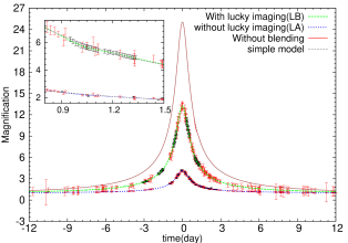
To clarify how much this strategy improves the quality of the planetary signal in microlensing light curves, we compare reconstructed light curve which has the highest amount of $\mathrm{\Delta\chi^{2}}$, i.e. that light curve corresponding to $\mathrm{\Omega=0.26~{}arcsec^{2}}$ after shifting to the least blending effect, with the original light curve taken from the normal cameras (shown in Figure 6). We called the former light curve before shifting the other data points by LB and the later one after shifting with LA. Figure (11) shows these light curves with simulated data points with their error bars, the theoretical light curve with no blending effect (red solid curve) and the best-fitted simple Paczyński microlensing model (gray dashed curves). The planetary signals of these light curves is zoomed in the inset of the figure. The Lucky Imaging camera decreases the blending effect, but increases the photometric uncertainties a bit (due to shifting process) and improves the detectability of the planetary signal (see Table 2). Here, the ratio of the blending parameters of these two light curves is $\mathrm{\alpha_{1}=3.9}$ which means that the blending effect in the LB light curve decreases by a factor of $\mathrm{1/\alpha_{1}}$.

Figure 12: The contour lines of planet detection efficiency for some of blended events from OGLE 2012 microlensing events. In the left panel we use the normal camera on the Danish telescope and in the right panel, we assume the Danish telescope is occupied with a Lucky camera and the introduced strategy is used to make light curves. For converting $\mathrm{\varepsilon(d,q)}$ to $\mathrm{\varepsilon(s,m_{p})}$ we use the typical amounts for the the mass of the primary lens $\mathrm{M_{l}=0.3M_{\odot}}$, the distances of the lens and source from the observer $\mathrm{D_{s}=8.5~{}kpc}$ and $\mathrm{D_{l}=6.5~{}kpc}$.

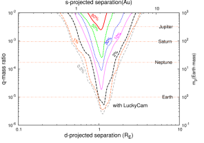
4 Planet detection efficiency

We continue our study to estimate the fraction of planets that can be detected by a typical microlensing event if we use the Lucky camera according to the strategy discussed in the previous section. We adopt the formalism introduced by Gaudi & Sackett (2000a,b) for detection efficiency calculation of real microlensing events with the blending effect.

We consider some of OGLE microlensing events with non-zero blending effects. We calculate the planet detection efficiency of every event and finally overlap them. For each event, we pick up its parameters from fitting process: i.e. the Einstein crossing time $\mathrm{t_{E}}$, the time of the closest approach $\mathrm{t_{0}}$, the lens impact parameter $\mathrm{u_{0}}$, the blending parameter $\mathrm{b}$ and the baseline flux $\mathrm{F_{bg}}$. The apparent source magnitude, $\mathrm{m_{\star}}$, can be obtained according to the blending parameter and the baseline flux. To indicate the source star radius of each microlensing event, we first specify the type of the source according to its apparent magnitude. Indeed, amongst the observed microlensing targets, there is a bimodal distribution for the source star magnitude, corresponding to bright giants on one side and highly-magnified faint main-sequence stars on the other side Cassan et al. (2012). The transition magnitude between these two types of giant and main-sequence stars is $17$ mag. We consider $\mathrm{R_{\star}=10R_{\odot}}$ for the former and $\mathrm{R_{\star}=R_{\odot}}$ for the latter, where $\mathrm{R_{\odot}}$ is the sun radius. For indicating the projected source radius on the lens plane $\mathrm{\rho_{\star}}$, we need to determine the Einstein radius and the lens-source relative distances from observer $\mathrm{x=D_{l}/D_{s}}$.

Estimations of these two parameters as well as indication of the lens mass are done according to the probability density of these parameters versus the Einstein crossing time which is plotted in Figure (5) of Dominik (2006). Two last parameters are times when the first $\mathrm{(t_{min})}$ and the last $\mathrm{(t_{max})}$ data points are taken by the Lucky Imaging camera for each light curves. Since a trigger is necessary to start observations it makes sense to continue following microlensing events further down after the peak, we adopt to start taking data points at $\mathrm{A_{obs}=1.5}$ and to stop at $\mathrm{A_{obs}=1.06}$.

For each event, the parameters of the planetary system, $\mathrm{q}$ and $\mathrm{d}$, change uniformly in the logarithmic scale over the ranges of $\mathrm{q\in[10^{-6},10^{-2}]}$ and $\mathrm{d\in[0.1,10]}$ with steps $\mathrm{\Delta\log q=0.0625}$ and $\mathrm{\Delta\log d=0.03125}$, respectively. The angle between the trajectory of the source with respect to the binary axis changes in the range of $\mathrm{\theta\in[0,360^{\circ}]}$ with the steps of $\mathrm{\Delta\theta=0.36^{\circ}}$.

For each configuration of lenses in terms of $\mathrm{q}$ and $\mathrm{d}$, the planet detection efficiency $\mathrm{\varepsilon(q,d)}$ is obtained for all the possible source trajectories $\mathrm{(0<\theta<2\pi)}$ which is given by:

$$\varepsilon(q,d)=\frac{1}{2\pi}\int_{0}^{2\pi}\Theta(q,d)d\theta.$$ (24)

where $\mathrm{\Theta}$ is a step function and is calculated for each simulated planetary microlensing event corresponding to given amounts of $\mathrm{(d,q,\theta)}$. We apply this function when in the related light curve four consecutive data points are located above (or below) the Paczyński light curve with more than $\mathrm{2\sigma}$ deviation. These points should be in the same side with respect to the Paczyński light curve. Otherwise, this function is set to be zero.

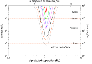
Having performed the simulation, in Figure (12) we compare the efficiency function of the planet detection using the standard camera in the Danish telescope (left panel) and the Lucky Imaging camera (right panel). For converting $\mathrm{\varepsilon(d,q)}$ to $\mathrm{\varepsilon(s,m_{p})}$ we use typical values for the the mass of the primary lens $\mathrm{M_{l}=0.3M_{\odot}}$, the distances of the source and the lens from the observer $\mathrm{D_{s}=8.5~{}kpc}$ and $\mathrm{D_{l}=6.5~{}kpc}$, where $\mathrm{s}$ is the projected separation in the Astronomical Unit (AU) and $\mathrm{m_{p}}$ is the planet mass. Comparing these two figures shows that the Lucky Imaging camera improves the planet detection efficiency in a crowded Field. Noting that we consider only microlensing events with non-zero blending effect. For example a Neptune-mass planet in the resonance regime can be detected with $30$ per cent chance with the Lucky camera compare to the normal camera with $10$ per cent probability. Also, we obtain the detection efficiency of an Earth-mass planet in the resonance regime is more than $\mathrm{\varepsilon\sim 2}$ per cent with the Lucky camera while with the normal camera this detection efficiency is about $\mathrm{0.5\%}$ in a crowded-field. If the abundance of Earth-mass planets is high (which is probable according to Cassan et al. 2012), a considerable number of Earth-mass planets in the resonance regime would be expected for detection with this method.

5 Conclusions

In this work we have investigated the advantage of using Lucky Imaging for exoplanet detection via the microlensing method. The Lucky Imaging method is a technique where cameras take series of images faster than the time scale of atmospheric turbulence. The selected best images where wave-fronts are not distorted are re-centered and combined to improve the final image.

We have simulated microlensing events observed with the Lucky camera on Danish $1.54$-m telescope accompanied by normal CCD cameras with other telescopes and in this regard introduced an observational strategy. We propose to fix the PSF area of the source star for a fixed photometric precision for all data points in a microlensing event. For a fixed PSF area in the Lucky camera the blending of the source star is fixed. We have two sets of data points with different blending parameters one for the normal camera and the other one with the Lucky camera. We propose shifting the low quality blending data points to the high quality data points by calculating the ratio of their blending parameters (i.e. $\mathrm{\alpha}$) in equation (19). Re-positioning some of data points over a microlensing light curve imposes an uncertainty for the shifted data points in which these uncertainties decrease by the PSF area. On the other hand we get fewer data points throughout the light curve as we decrease the PSF area (see Table 1).

In order to address that problem, we propose to produce data points from the Lucky camera with the least PSF area. Since these Lucky images are stored in our database, we repeated analyzing Lucky camera data with larger $\mathrm{\Omega}$s, resulted in increasing the data points in the light curve. From the $\mathrm{\alpha}$ parameter in each data set of the Lucky camera, we shifted the corresponding data points to that of the highest $\mathrm{\alpha}$. Finally, we produced a light curve with the minimum blending effect and highest number of data points. In our analysis we have the best light curve according to the maximum value of $\mathrm{\Delta\chi^{2}}$, representing the difference between $\mathrm{\chi^{2}}$ from fitting a simple microlensing light curve and a planetary microlensing light curve.

We have also studied the improvement of the planetary detection efficiency using the Lucky Imaging camera. In this regard, we have microlensing events of OGLE 2012 data with nonzero blending effect, calculated their planetary detection efficiencies and overlapped their detection efficiencies. We obtained the detecting efficiency of an Earth-mass planet with the Lucky camera in the resonance regime increases up to $\mathrm{\sim 2\%}$ while this efficiency with the normal cameras is about $\mathrm{0.5\%}$ in a crowded field. If the abundance of these planets is high (which is probable according to Cassan et al. 2012), the number of detectable Earth-mass planets whose positions are projected in the resonance regime will be four times more with using this method.

Acknowledgment Works by SS and SR were supported by the grant $\mathrm{94017434}$ from the Iran National Science Foundation (INSF). We thank the referee for useful comments and suggestions which certainly improved the manuscript.

References

- Baldwin et al. (2001) Baldwin J. E., Tubbs, R.N., Cox, G.C., Mackay C.D., Wilson, R.W. & Andersen, M.I., 2001, A&A, 368,L1.
- Batista et al. (2011) Batista, V., Gould, A., Dieters, S., et al. 2011, A&A, 529, L102.
- Beaulieu et al. (2006) Beaulieu, J.-P., Bennett, D. P., Fouqué, P., et al. 2006, Nature, 439, L437.
- Bennett & Rhie (1996) Bennett, D.P., & Rhie, S.H. 1996, ApJ, 472, L660.
- Bennett & Rhie (2002) Bennett, D.P., & Rhie, S.H. 2002, ApJ, 574, L985.
- Bessell (1979) Bessell, M.S. 1979, PASP, 91, L589.
- Bramich (2008) Bramish D. M., 2008, MNRAS, 386, L77.
- Cardelli et al. (1989) Cardelli J. A., Clayton G. C. & Mathis J. S., 1989, ApJ, 345, L245.
- Cassan et al. (2012) Cassan, A., Kubas, D., Beaulieu, J.-P., et al., 2012, Nature, 481, L167.
- Cecil & Rashkeev (2007) Cecil, G., Rashkeev, D., 2007, AJ, 134, L1468.
- Chang & Refsdal (1979) Chang K., Refsdal S., 1979, Nature, 282, L561.
- Dantowitz et al. (2000) Dantowitz, R.F., Teare, S.W. & Kozubal, M.J., 2000, AJ, 119, L2455.
- Dominik (2006) Dominik, M., 2006, MNRAS 367, L669.
- Dominik (2007) Dominik, M., 2007, MNRAS, 377, L1679.
- Dominik et al. (2008) Dominik M., Horne K., Allan A., et al., 2008, Astronomische Nachrichten, 329, L248.
- Dominik et al. (2010) Dominik, M., et. al., 2010, Astron. Nachr./AN, 331, 7, L671.
- Dwek et al. (1995) Dwek, E., Arendt, R.G., Hauser, M.G., et al., 1995, ApJ, 445, L716.
- Einstein (1936) Einstein A., 1936, Science, 84, L506.
- Fried (1978) Fried, D.L. 1978, J. Opt. Soc. Am., 68, L1651.
- (20) Gaudi, S.B. & Sackett, P.D., 2000a, ApJ, 528, L65.
- (21) Gaudi, S.B. & Sackett, P.D., 2000b, ApJ, 566, L463.
- Griest & Safizadeh (1998) Griest, K. & Safizadeh, N., 1998, ApJ, 500, L37.
- Gonzalez et al. (2012) Gonzalez O. A., Rejkuba M., Zoccali M., et al., 2012, A & A, 543, L13.
- Gould & Loeb (1992) Gould, A., & Loeb, A. 1992, ApJ, 396, L104.
- Hecquent & Coupinot (1985) Hecquent, J., Coupinot, G., 1985, Journal of Optics, 16, L21.
- Hufnagel & Stanley (1966) Hufnagel R. E., Stanley N.R., 1964, J. Opt. Soc. Am., 54, 52.
- Law et al. (2006) Law, N.M., Mackay C.D. & Baldwin J.E. 2006, A & A, 446, L739.
- Law et al. (2009) Law, N.M., et al. 2009, ApJ, 692, L924.
- Liebes (1964) Liebes, Jr.S., 1964, Phys. Rev., 133, L835.
- Mao & Paczyński (1991) Mao, S., & Paczyński, B. 1991, ApJ, 374, L37.
- Muraki et al. (2011) Muraki, Y., Han, C., Bennett, D. P., et al. 2011, ApJ, 741, L22.
- Nataf et al. (2013) Nataf D. M., Gould A., Fouqué P., et al., 2013, ApJ, 769, L88.
- Paczyński (1986) Paczyński B., 1986, ApJ, 304, L1.
- Paczyński (1996) Paczyński B., 1996, ARA & A, 34, L419.
- Quintana et al. (2014) Quintana E.V., Barclay T., Raymond S.N., et al., 2014, Science, 344, 6181.
- Robin et al. (2003) Robin, A.C., Reylé, C., Derrière, S., Picaud, S., 2003, A& A, 409, L523.
- Sajadian (2015) Sajadian, S., 2015, AJ, 149, L147.
- Shin et al. (2012) Shin, I.-G., Choi, J.-Y., Park, S.-Y., et al. 2012, ApJ, 746, L127.
- Skottfelt et al. (2015) Skottfelt J., Bramich D.M., Hundertmark M., et al., 2015, A & A, 574, A54.
- Strehl (1895) Strehl, K. 1895, Aplanatische und fehlerhafte Abbildung im Fernrohr, Zeitschrift fur Instrumentenkunde, L362.
- Sumi et al. (2010) Sumi, T., Bennett, D. P., Bond, I. A., et al. 2010, ApJ, 710, L1641.
- Vermaak (2000) Vermaak P., 2000, MNRAS, 319, L1011.
- Weingartner & Draine (2001) Weingartner, J. C.& Draine, B. T. 2001, ApJ 548, L296.
- Wyrzykowski et al. (2014) Wyrzykowski, Ł., et al., 2014, arXiv:1405.3134.