Probing superfluidity in a quasi two-dimensional Bose gas through its local dynamics
Abstract
We report direct evidence of superfluidity in a quasi two-dimensional Bose gas by observing its dynamical response to a collective excitation. Relying on a novel local correlation analysis, we are able to probe inhomogeneous clouds and reveal their local dynamics. We identify in this way the superfluid and thermal phases inside the gas and locate the boundary at which the Berezinskii–Kosterlitz–Thouless crossover occurs. This new analysis also allows to evidence the coupling of the two fluids which induces at finite temperatures damping rates larger than the usual Landau damping.
Superfluidity is one of the most fascinating expressions of quantum mechanics at the macroscopic level. It manifests itself through specific dynamical properties, giving rise to collective effects as diverse as quantized vortices or second sound Leggett (1999). First observed in liquid helium Wilks and Betts (1987), superfluidity has also been shown to occur for polaritons in semi-conductor micro-cavities or weakly interacting quantum gases Bennemann and Ketterson (2013). Thanks to mature imaging techniques and a high degree of control over their parameters, the latter have proven to be particularly well suited for evidencing key features of superfluids: their linear excitation spectrum at low momentum Ozeri et al. (2005) as well as the existence of a finite critical velocity have been observed Landau (1941); Raman et al. (1999); Desbuquois et al. (2012). Moreover when set into rotation quantum gases display vortices Madison et al. (2001); Abo-Shaeer et al. (2001) and present specific collective modes Stringari (1996); Guéry-Odelin and Stringari (1999). Yet, extracting relevant information from the dynamics of these systems still represents an experimental challenge.
Properties of quantum gases are fully determined by the knowledge of their density and temperature. Hence, in order to explore different physical regimes, these quantities may have to be varied over a large range of values. While for homogeneous systems each repetition of an experiment will address a single point of this phase space, inhomogeneous quantum gases readily experience different regimes locally. This is the framework of the local density approximation (LDA), which has been extensively exploited while exploring physics of quantum gases at equilibrium. It has allowed for instance the determination of the equation of state of a Fermi gas at unitarity Nascimbène et al. (2010) and of a two-dimensional (2D) Bose gas both in the weakly and strongly interacting regimes Rath et al. (2010); Yefsah et al. (2011); Ha et al. (2013). In the same spirit, density fluctuations of a quasi-one-dimensional Bose gas have been described from the quasi-condensate to the nearly ideal gas regime Esteve et al. (2006).
In this work, we extend this approach to the in situ study of the dynamical properties of an inhomogeneous quantum gas. We apply a novel local correlation analysis to probe the superfluidity of a quasi-2D Bose gas, observing its response to the so-called scissors excitation Guéry-Odelin and Stringari (1999); Maragò et al. (2000). It allows us to identify and locate the superfluid and normal phases within the system. In addition, at finite temperature we evidence a collisional coupling between them. In a sense, our scheme relying on the weak global excitation of a gas close to equilibrium probed locally is symmetric to the recent measurement of the critical velocity in an inhomogeneous quasi-2D Bose gas, where the effect of a strong local perturbation is probed through a global observable, the total heat deposited over the whole cloud Desbuquois et al. (2012).
The reduction to low dimensions strongly affects the physics of the collective properties of a quantum system Pricoupenko et al. (2003); Bloch et al. (2008). In particular, in two dimensions, thermal phase fluctuations destroy long range order Mermin and Wagner (1966) and prevent the occurrence of Bose-Einstein condensation (BEC) in a homogeneous Bose gas at any finite temperature Posazhennikova (2006). On the other hand, these systems undergo a Berezinskii–Kosterlitz–Thouless (BKT) phase transition to a superfluid state Berezinskii (1971); Kosterlitz and Thouless (1973); Bishop and Reppy (1978). This still holds for quantum gases confined in harmonic traps Holzmann and Krauth (2008) as evidenced experimentally for quasi-2D Bose gases through the algebraic decay of their phase coherence Hadzibabic et al. (2006). Here, we directly locate the boundary where the superfluid fraction vanishes across the BKT crossover through local correlation analysis.


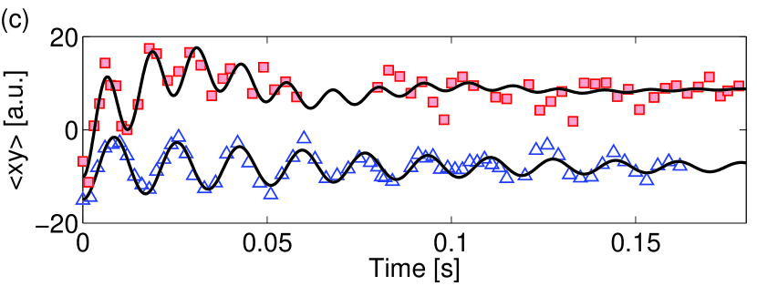
The starting point for our experiments is a partially degenerate Bose gas of 87Rb atoms produced in a radio-frequency (rf) dressed quadrupole trap Merloti et al. (2013), loaded from an hybrid trap Dubessy et al. (2012). For our experimental parameters the measured vertical trapping frequency is much larger than the in-plane trapping frequencies and , resulting in a pancake shaped atomic cloud. The trap in-plane geometry, defined by the direction of the eigenaxes and the anisotropy , is controlled by the rf polarization.
We prepare different samples by varying the total atom number and temperature. As both the temperature and the chemical potential are comparable to the vertical oscillator energy level spacing , the system is in the quasi-2D regime, and the effective dimensionless 2D interaction constant is Petrov et al. (2000), where is the scattering length, the vertical harmonic oscillator length and the atomic mass. For most of our datasets the fraction of atoms out of the vertical oscillator groundstate is smaller than , despite the relatively high temperatures and chemical potentials111See supplementary material for details on the imaging techniques, data processing and models. (with respect to ). Therefore the system is well described by coupled 2D manifolds and exhibits 2D physics. Specifically, the BKT transition is expected to occur in our trap at a phase space density for a reduced chemical potential equal to Prokof’ev et al. (2001). These critical values increase slightly when the effect of the population in the transverse excited states at is taken into account Holzmann et al. (2010). The samples are prepared with a reduced chemical potential in the range , on both sides of the expected threshold Note (1).
We excite the scissors oscillations by suddenly changing the orientation of the horizontal confinement axes by , while keeping the trap frequencies constant Dubessy et al. (2014), see figure 1(a). The superfluid and thermal fractions of the cloud are subsequently expected to oscillate at different frequencies: for a normal gas close to the collisionless regime and for the superfluid Guéry-Odelin and Stringari (1999). We typically record one hundred in situ pictures of the atoms after different holding times, spanning about . In order to study the scissors mode at finite temperature, it is essential to be able to discriminate between the superfluid and thermal phases Maragò et al. (2001). However a direct fit of the 2D in situ density profiles by a bi-modal function is quite imprecise because the typical width over which they extend are comparable.
Inspired by the theoretical works which use the average as an observable of the scissors mode excitation Guéry-Odelin and Stringari (1999); Jackson and Zaremba (2001); Simula et al. (2008), we use an efficient algorithm to extract from our data Note (1). For all of our datasets presents damped oscillations as illustrated in figure 1(c). In order to quantitatively analyze this signal, we take advantage of the classical description of the scissors oscillations Guéry-Odelin and Stringari (1999). In this framework the complex oscillation frequencies of are parametrized by a characteristic relaxation time :
| (1) |
In the hydrodynamic limit where vanishes, this model also describes the scissors mode in a superfluid Guéry-Odelin and Stringari (1999). Applying this prediction to our data, we are able to fit Note (1) the value of and deduce the frequencies and damping rates of the oscillations relying on the constraints of equation (1). In this way, we perform a double frequency fit with only three parameters (amplitude, offset and ). The model always predicts two frequencies, corresponding to an upper branch and a lower branch. The former spans frequencies in the range while the latter spans . We found this method to be more accurate than a fit to a sum of two damped cosines which requires at least nine free parameters, in particular for the determination of the lowest, highly damped, frequency. We checked that the fit constrained by equation (1) introduces no bias and that both models give the same results Note (1).
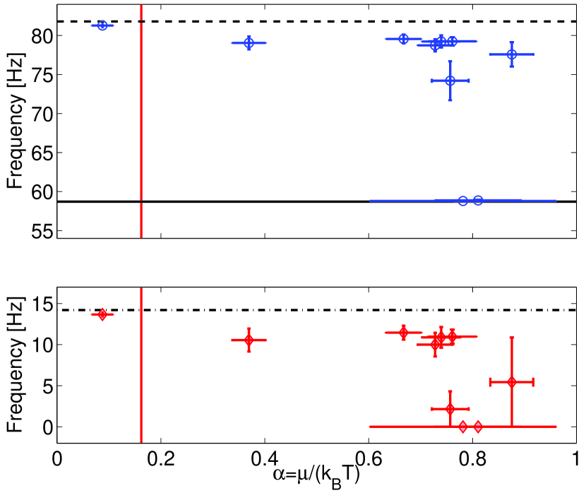
Figure 2 reports the frequencies found as a function of the reduced chemical potential . Below the BKT transition (, leftmost point of the graph), the two frequencies are very close to, but slightly below, the classical prediction . This, together with the large observed damping rates (see figure 1(c)), indicates that the gas is not fully in the collisionless regime, which would require Guéry-Odelin and Stringari (1999). For samples above the BKT transition () we find either a single frequency close to or two frequencies, shifted below the collisionless frequencies . Our data are consistent with an increase of the upper frequency from to when decreases, in agreement with 2D dynamical classical field simulations Simula et al. (2008), and in stark contrast with what was observed in three-dimensional experiments Maragò et al. (2001). We note however that the simple criterion based on the critical value is not sufficient to describe our datasets: in particular the thermal frequencies are still observable beyond . The global observable therefore fails to evidence the normal to superfluid crossover. Indeed, in these conditions the superfluid and normal phases coexist in the trap and the simple picture of equation (1) does not capture all the dynamics. Moreover, as the observable is computed over the whole sample, both phases are combined in the total signal and it is difficult to isolate their respective signature.
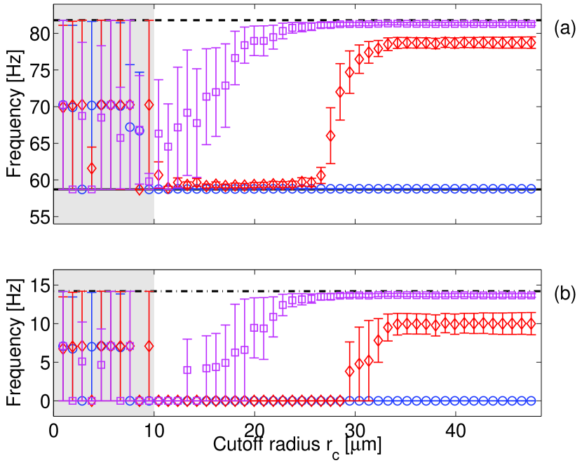

In order to overcome this issue we introduce the concept of local correlation analysis. In the spirit of LDA, we define the rescaled radius , following a 2D isodensity path around the trap center. We compute a partial average evaluated by including only the pixels at a rescaled distance . In this way we expect to isolate the superfluid phase which is located at smaller .
Figure 3 presents the frequencies found as a function of the cut-off radius , for three of the datasets. Below a cutoff radius of there is no clear oscillation (indicated by the large error bars). This reflects the fact that the scissors excitation is a surface mode and does not affect the core of the cloud. Beyond this cutoff radius, we observe in most of the datasets a central region oscillating at a single frequency, in good agreement with the hydrodynamic prediction , which was not apparent in the global analysis. For larger radii, we recover the results of the global analysis, showing that the contribution of the central region to the total signal is small, even if the density is higher at the center. The radius at which the crossover between these two regimes occurs depends on . As discussed below, this result is a direct evidence of the coexistence of normal and superfluid scissors excitations at finite temperature in our system.
To get more accurate results, we reduce further the region of interest to a thin annulus centered on , with a width pixels, thus probing an isodensity region of the cloud. Figure 4 displays the frequencies measured for this partial average as a function of , for , corresponding to one of the datasets of figure 3.
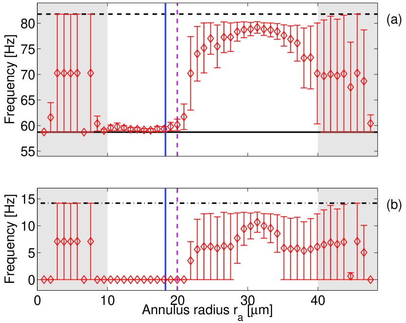

The larger error bars result from a smaller number of pixels involved in the average. This local analysis is even more sensitive to frequency shifts and allows a more accurate determination of the position of the boundary between the two phases at .
We attribute the hydrodynamic part of the gas present at the center to the superfluid phase of the degenerate quasi-2D Bose gas. One may wonder if a hydrodynamic classical gas at high density could explain our observation. From the independent measurement of the equilibrium values of and , we evaluate the scaled distance from the trap center at which the reduced local chemical potential , where , reaches the critical value for the BKT transition Holzmann et al. (2010). This is indicated by the vertical blue solid line in figure 4, in good agreement with our observed crossover. The small discrepancy could be explained in two ways. First, close to the critical radius, the finite extension of our local probe averages the signal over both the superfluid and normal regions. Second, finite size effects for a trapped cloud, away from the thermodynamic limit, modify the position of the expected boundary anyway. Indeed, a Quantum Monte Carlo simulation of a quasi two-dimensional trapped Bose gas with our parameters222Markus Holzmann, private communication. has shown that the normal to superfluid crossover is broadened by about in the sample, resulting in a non-zero superfluid fraction beyond the critical radius predicted by the LDA. We are thus confident that we observe the superfluid to classical transition signature in the dynamical response of the gas.
We now come to the interpretation of the local relaxation time deduced from the local analysis. We find that its value is in good agreement with the inverse of the local collision rate evaluated in the confinement dominated three-dimensional regime Petrov and Shlyapnikov (2001), where is the measured average 2D density on the annulus. This supports the use of equation (1) to describe the local dynamics. We point out that our analysis could give access to a local relaxation time of the excitation, a key ingredient in finite temperature two-fluid models Williams and Griffin (2001); Nikuni (2002).
Conversely we use the measured to estimate the local collision rate and hence the local phase space density, knowing the sample temperature. The vertical dashed magenta line in figure 4 indicates the radius at which this estimated local phase space density becomes higher than the BKT critical phase space density computed for this quasi-2D gas Holzmann et al. (2010). The analysis of the dynamics thus confirms the location of the boundary between the superfluid and normal phases.
We now turn to a quantitative analysis of the damping rates of the local correlations. We will only consider the upper frequency branch, sketched on figure 5(a), as the lower frequency is highly damped in our experiments. In order to get a reliable estimate of the frequency and damping rates of the scissors oscillation for both the central and outer regions, we exclude the crossover area and compute the averages over a disc for the central part and over a large annulus for the outer part, as illustrated on figure 5(c). Figure 5(b) compares the measured reduced damping rate of the scissors oscillations to the reduced Landau damping Pitaevskii and Stringari (1997); Fedichev et al. (1998):
| (2) |
where is the sound velocity for a pancake-shaped Bose gas De Rosi and Stringari (2015).
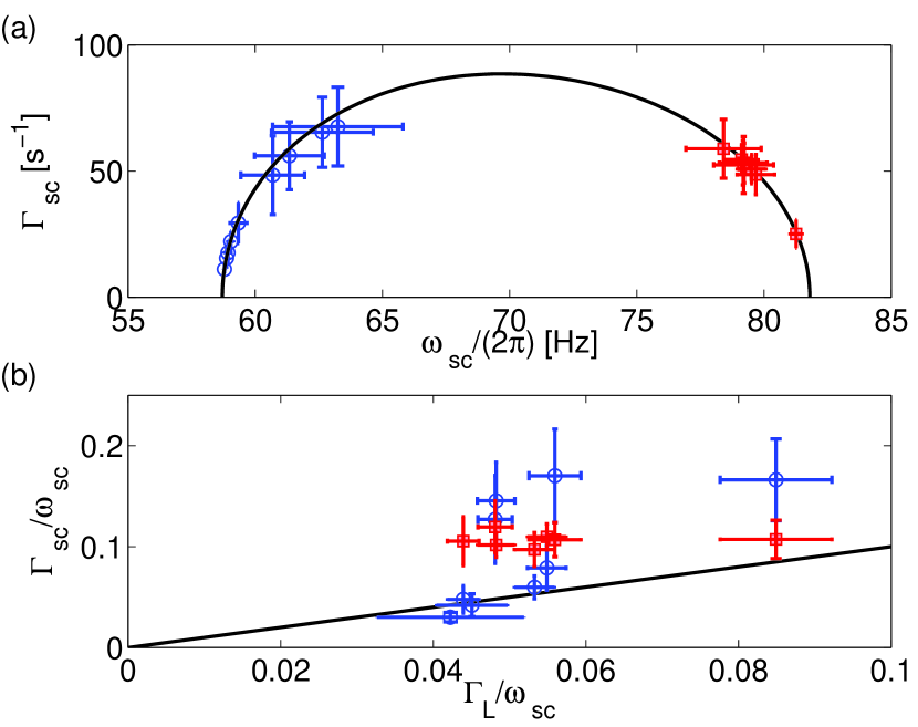

For our coldest samples the measured damping rate for the superfluid phase is close to the damping predicted by equation (2). However for the datasets with a large thermal fraction, the damping in the superfluid phase deviates from the predicted Landau damping and is of the same order of magnitude than the damping in the normal phase, suggesting that this additional damping originates from collisional coupling to the normal gas Williams and Griffin (2001). The reduced damping rate in the normal phase is approximately constant for all our datasets. We note that in our 2D geometry the abnormal damping cannot be explained by a resonant Beliaev coupling to other modes as observed in three-dimensional experiments Hodby et al. (2001).
In conclusion we have studied the dynamics of a quasi-2D Bose gas near the BKT transition. We have shown the coexistence of a superfluid fraction and a thermal part by a direct, in situ, local analysis of its dynamical behavior. We use the frequency of the scissors mode as a local probe of superfluidity. Whereas a global analysis of the data fails to reveal the coexistence of the superfluid and normal oscillations, we demonstrate a new local correlation analysis, reminiscent of the local density approximation, which allows to locate the normal to superfluid transition, using a purely dynamical criterion. The position of the boundary is in good agreement with the crossover expected from the equilibrium properties of the gas. In principle it should be possible with this local probe to observe the superfluid density jump at the BKT transition Nelson and Kosterlitz (1977); Bishop and Reppy (1978). This motivates future numerical studies of finite temperature dynamics to establish quantitatively the relation between local scissors frequency and local superfluid fraction.
Local correlation analysis could also be applied to numerical simulations. In particular, the local measurement of relaxation times would be useful to compare experiments to numerical calculations at finite temperature. We expect this new kind of local diagnosis to shed new light on the study of out-of-equilibrium systems.
Acknowledgements.
We thank M. Holzmann for enlightening discussions and for providing us with the QMC simulations of our experiment, S. Stringari for helpful suggestions and acknowledge stimulating discussions with B. Laburthe-Tolra. We thank D. Guéry-Odelin for a critical reading of the manuscript. We acknowledge financial support from ANR project SuperRing (ANR-15-CE30-0012-01). LPL is a member of Institut Francilien de Recherche sur les Atomes Froids (IFRAF).Supplementary material
.1 Image processing
The determination of the equilibrium properties of the cloud follows the approach described in reference Hadzibabic et al. (2008). Prior to the excitation we take an in situ picture of the atoms at rest in the initial trap using a low intensity () imaging pulse, to recover correctly the low density profile of the thermal wings. We then adjust this density profile by a self consistently determined Hartree-Fock mean field model including up to ten excited states manifolds. From this procedure we deduce the chemical potential and temperature of the cloud Hadzibabic et al. (2008). The total atom number and detection efficiency are calibrated independently using an auxiliary time of flight imaging system observing the atoms at lower density from the side Dubessy et al. (2012). The equilibrium parameters for the different datasets are summarized in table 1.
| Dataset | (Hz) | (nK) | ||
|---|---|---|---|---|
| 1 | 0.90 | |||
| 2 | 0.88 | |||
| 3 | 0.86 | |||
| 4 | 0.88 | |||
| 5 | 0.86 | |||
| 6 | 0.82 | |||
| 7 | 0.81 | |||
| 8 | 0.80 | |||
| 9 | 0.42 | |||
| 10 | 0.59 |
The number of atoms in the groundstate of the vertical harmonic oscillator is estimated from the values of the chemical potential and temperature using an hybrid Thomas-Fermi plus Hartree-Fock mean field model that allows to compute the populations in the first ten vertical oscillator manifolds. Since a majority of the atoms are in the groundstate the system is in the quasi two-dimensional regime.
After the excitation, we record the atomic density after a variable delay time using a saturating imaging pulse () Reinaudi et al. (2007). We are thus able to resolve both the low density thermal wings of the cloud and the high density degenerate core. Our home-made imaging system has a resolution of and an effective pixel size of in object space.
In order to compute the relevant density weighted average values , , , and , it is necessary to remove the imaging noise which does not correspond to real atomic signal. We proceed as follows. For a square picture, and a small ellipsoidal cloud, about half the pixels do not represent atoms and therefore contain information only about the noise. This appears clearly if one plots the histogram of the picture, as we do in figure 6.
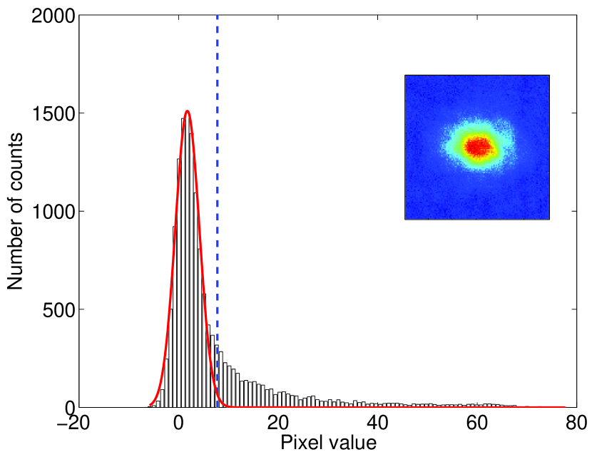
We identify a large contribution due to the background, with a low value of signal, and a smaller contribution due to the data, at larger signal values. From a Gaussian fit to the background contribution, we estimate a signal threshold ( of the Gaussian) above which we can neglect the noise. We then cancel the contribution of all pixels having a value lower than the threshold. Note that this process also filters a few relevant pixels, but it greatly improves the signal to noise ratio. We checked that the results are insensitive to the exact position of the threshold.
After this noise removal procedure, we compute the values of , , , and for each picture, where and are the coordinates of the pixels in the camera frame. By adjusting the two-dimensional center of mass motion of the cloud we find the trap frequencies, the trap center, and the orientation of the axes relative to the camera. Then by combining with appropriate weights the second order moments we extract the values in the trap frame.
.2 Scissors mode classical model
In this section we describe the fitting procedure used in the main paper to extract the frequencies and relaxation times of the scissors oscillations. We start from the following set of coupled equations describing the classical scissors oscillations Guéry-Odelin and Stringari (1999):
| (3a) | |||||
| (3b) | |||||
| (3c) | |||||
| (3d) | |||||
We denote the solution of equations (3) with initial conditions: (an arbitrary non zero value), and . We use the time-dependent function as a model to fit our experimental data, with , and as free real parameters. For small values of this model is close to a damped cosine, with frequency , while for large values of this model is close to a sum of two damped cosines with frequencies close to . In both cases the damping depends on the exact value of . Once we have determined the value of from the fit, we solve equation (1) of the main paper to find the corresponding frequency and damping rate.
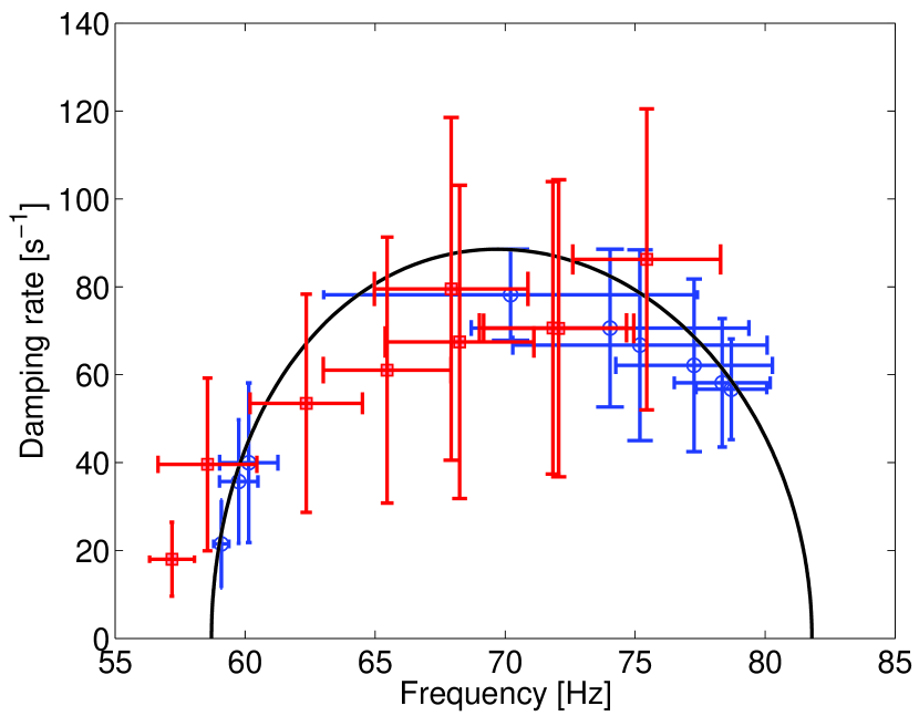
Figure 7 displays the damping rates and frequencies found for different radii for the same dataset as in figure 4, using two fitting methods: the one described above and a simple sum of two damped cosines. Both models give results close to the prediction of equation (1) (considering the error bars). As mentioned before the former model has been derived from the predictions of equation (1) and therefore the points must fall near the theoretical curve. However the latter model do not make any kind of assumption constraining the relative values of the damping rate and the frequency and yet agrees with the same theoretical prediction. Therefore we conclude that equation (1) quantitatively describes the scissors oscillations found with our local correlation analysis scheme. Using our model fit enables to reduce the error bars and thus to extract the low frequency branch from the noise.
References
- Leggett (1999) A. J. Leggett, Rev. Mod. Phys. 71, S318 (1999).
- Wilks and Betts (1987) J. Wilks and D. Betts, An Introduction to Liquid Helium (Clarendon Press (Oxford), 1987).
- Bennemann and Ketterson (2013) K. H. Bennemann and J. B. Ketterson, eds., Novel superfluids (Oxford University Press, 2013).
- Ozeri et al. (2005) R. Ozeri, N. Katz, J. Steinhauer, and N. Davidson, Rev. Mod. Phys. 77, 187 (2005).
- Landau (1941) L. Landau, Phys. Rev. 60, 356 (1941).
- Raman et al. (1999) C. Raman, M. Köhl, R. Onofrio, D. S. Durfee, C. E. Kuklewicz, Z. Hadzibabic, and W. Ketterle, Phys. Rev. Lett. 83, 2502 (1999).
- Desbuquois et al. (2012) R. Desbuquois, L. Chomaz, T. Yefsah, J. Léonard, J. Beugnon, C. Weitenberg, and J. Dalibard, Nat. Phys. 8, 645 (2012).
- Madison et al. (2001) K. W. Madison, F. Chevy, V. Bretin, and J. Dalibard, Phys. Rev. Lett. 86, 4443 (2001).
- Abo-Shaeer et al. (2001) J. R. Abo-Shaeer, C. Raman, J. M. Vogels, and W. Ketterle, Science (80-. ). 292, 476 (2001).
- Stringari (1996) S. Stringari, Phys. Rev. Lett. 77, 2360 (1996).
- Guéry-Odelin and Stringari (1999) D. Guéry-Odelin and S. Stringari, Phys. Rev. Lett. 83, 4452 (1999).
- Nascimbène et al. (2010) S. Nascimbène, N. Navon, K. J. Jiang, F. Chevy, and C. Salomon, Nature 463, 1057 (2010).
- Rath et al. (2010) S. P. Rath, T. Yefsah, K. J. Günter, M. Cheneau, R. Desbuquois, M. Holzmann, W. Krauth, and J. Dalibard, Phys. Rev. A 82, 013609 (2010).
- Yefsah et al. (2011) T. Yefsah, R. Desbuquois, L. Chomaz, K. J. Günter, and J. Dalibard, Phys. Rev. Lett. 107, 130401 (2011).
- Ha et al. (2013) L.-C. Ha, C.-L. Hung, X. Zhang, U. Eismann, S.-K. Tung, and C. Chin, Phys. Rev. Lett. 110, 145302 (2013).
- Esteve et al. (2006) J. Esteve, J. B. Trebbia, T. Schumm, a. Aspect, C. I. Westbrook, and I. Bouchoule, Phys. Rev. Lett. 96, 1 (2006).
- Maragò et al. (2000) O. M. Maragò, S. A. Hopkins, J. Arlt, E. Hodby, G. Hechenblaikner, and C. J. Foot, Phys. Rev. Lett. 84, 2056 (2000).
- Pricoupenko et al. (2003) L. Pricoupenko, H. Perrin, and M. Olshanii, eds., Quantum Gases in Low dimensions (Les Houches 2003) (J. Phys IV, 2003).
- Bloch et al. (2008) I. Bloch, J. Dalibard, and W. Zwerger, Rev. Mod. Phys. 80, 885 (2008).
- Mermin and Wagner (1966) N. D. Mermin and H. Wagner, Phys. Rev. Lett. 17, 1133 (1966).
- Posazhennikova (2006) A. Posazhennikova, Rev. Mod. Phys. 78, 1111 (2006).
- Berezinskii (1971) V. L. Berezinskii, J. Exp. Theor. Phys. 34, 610 (1971).
- Kosterlitz and Thouless (1973) J. M. Kosterlitz and D. J. Thouless, J. Phys. C Solid State Phys. 6, 1181 (1973).
- Bishop and Reppy (1978) D. J. Bishop and J. D. Reppy, Phys. Rev. Lett. 40, 1727 (1978).
- Holzmann and Krauth (2008) M. Holzmann and W. Krauth, Phys. Rev. Lett. 100, 190402 (2008).
- Hadzibabic et al. (2006) Z. Hadzibabic, P. Krüger, M. Cheneau, B. Battelier, and J. Dalibard, Nature 441, 1118 (2006).
- Merloti et al. (2013) K. Merloti, R. Dubessy, L. Longchambon, A. Perrin, P.-E. Pottie, V. Lorent, and H. Perrin, New J. Phys. 15, 033007 (2013).
- Dubessy et al. (2012) R. Dubessy, K. Merloti, L. Longchambon, P.-E. Pottie, T. Liennard, A. Perrin, V. Lorent, and H. Perrin, Phys. Rev. A 85, 013643 (2012).
- Petrov et al. (2000) D. S. Petrov, M. Holzmann, and G. V. Shlyapnikov, Phys. Rev. Lett. 84, 2551 (2000).
- Note (1) See Supplemental Material for details on the imaging techniques, data processing and models..
- Prokof’ev et al. (2001) N. Prokof’ev, O. Ruebenacker, and B. Svistunov, Phys. Rev. Lett. 87, 270402 (2001).
- Holzmann et al. (2010) M. Holzmann, M. Chevallier, and W. Krauth, Phys. Rev. A 81, 043622 (2010).
- Dubessy et al. (2014) R. Dubessy, C. De Rossi, T. Badr, L. Longchambon, and H. Perrin, New J. Phys. 16, 122001 (2014).
- Maragò et al. (2001) O. Maragò, G. Hechenblaikner, E. Hodby, and C. Foot, Phys. Rev. Lett. 86, 3938 (2001).
- Jackson and Zaremba (2001) B. Jackson and E. Zaremba, Phys. Rev. Lett. 87, 100404 (2001).
- Simula et al. (2008) T. P. Simula, M. J. Davis, and P. B. Blakie, Phys. Rev. A 77, 023618 (2008).
- Note (2) Markus Holzmann, private communication.
- Petrov and Shlyapnikov (2001) D. S. Petrov and G. V. Shlyapnikov, Phys. Rev. A 64, 012706 (2001).
- Williams and Griffin (2001) J. E. Williams and A. Griffin, Phys. Rev. A 63, 023612 (2001).
- Nikuni (2002) T. Nikuni, Phys. Rev. A 65, 033611 (2002).
- Pitaevskii and Stringari (1997) L. Pitaevskii and S. Stringari, Phys. Lett. A 235, 398 (1997).
- Fedichev et al. (1998) P. O. Fedichev, G. V. Shlyapnikov, and J. T. M. Walraven, Phys. Rev. Lett. 80, 2269 (1998).
- De Rosi and Stringari (2015) G. De Rosi and S. Stringari, Phys. Rev. A 92, 053617 (2015).
- Hodby et al. (2001) E. Hodby, O. M. Maragò, G. Hechenblaikner, and C. J. Foot, Phys. Rev. Lett. 86, 2196 (2001).
- Nelson and Kosterlitz (1977) D. R. Nelson and J. M. Kosterlitz, Phys. Rev. Lett. 39, 1201 (1977).
- Hadzibabic et al. (2008) Z. Hadzibabic, P. Krüger, M. Cheneau, S. P. Rath, and J. Dalibard, New J. Phys. 10, 045006 (2008).
- Reinaudi et al. (2007) G. Reinaudi, T. Lahaye, Z. Wang, and D. Guéry-Odelin, Opt. Lett. 32, 3143 (2007).