The VMC Survey. XIX. Classical Cepheids in the Small Magellanic Cloud
Abstract
The VISTA near-infrared survey of the Magellanic System (VMC) is collecting deep -band time-series photometry of pulsating variable stars hosted by the two Magellanic Clouds and their connecting Bridge. In this paper, we present light curves for a sample of 4172 Small Magellanic Cloud (SMC) Classical Cepheids (CCs). These data, complemented with literature values, allowed us to construct a variety of period–-luminosity (), period–-luminosity–-color (), and period-–Wesenheit () relationships, valid for Fundamental (F), First Overtone (FO) and Second Overtone (SO) pulsators. The relations involving bands are in agreement with their counterparts in the literature. As for the band, to our knowledge we present the first CC , , and relations ever derived using this filter. We also present the first near–infrared , , and relations for SO pulsators to date. We used to estimate the relative SMC–LMC distance and, in turn, the absolute distance to the SMC. For the former quantity we find a value of mag, in rather good agreement with other evaluations based on CCs, but significantly larger than the results obtained from older population II distance indicators. This discrepancy might be due to the different geometric distributions of young and old tracers in both Clouds. As for the absolute distance to the SMC, our best estimates are mag and mag, based on two distance measurements to the LMC, which rely on accurate CC and eclipsing Cepheid binary data, respectively.
Subject headings:
stars: variables: Cepheids; stars: oscillations; galaxies: Magellanic Clouds; cosmology: distance scaleI. Introduction
The Magellanic Clouds (MCs) are fundamental touchstones in the context of stellar populations and galactic evolution studies (see, e.g., Harris & Zaritsky, 2004, 2009; Ripepi et al., 2014a). Indeed, they are relatively close ( kpc Westerlund, 1997; Udalski et al., 1999), they are rich in stars of different ages, and their morphologies have been significantly affected by their dynamical interaction. In effect, there are clear signatures that the Small Magellanic Cloud (SMC), a gas-rich, dwarf irregular galaxy, is interacting with its neighbours, the Large Magellanic Cloud (LMC) and the Milky Way (MW). In particular, the MCs are connected by a Bridge dominated by Hi gas but which also contains a significant stellar content (e.g. Irwin et al., 1985; Harris, 2007). Like the Magellanic Stream, the Bridge may be the signature of the MCs’ mutual gravitational effects and/or the impact of the MW (e.g. Putman et al., 1998; Hammer et al., 2015). In addition, the SMC Wing, the part of the SMC main body extending asymmetrically towards the LMC (Shapley, 1940), could be the result of tidal interaction(s). Moreover, the bar of the SMC, traced by the galaxy’s young populations, appears highly asymmetric and elongated, with its northeastern portion closer to us than its southwestern part (e.g. Welch et al., 1987; Haschke et al., 2012; Rubele et al., 2015; Scowcroft et al., 2016). In general, the morphology of the SMC appears to depend on the age of the stellar population used as a probe (see, e.g. Cioni et al., 2000a; Zaritsky et al., 2000; Dobbie et al., 2014; Deb et al., 2015, and references therein). The study of the structure of the SMC is further complicated by the presence of a considerable line-of-sight depth variation in the galaxy. Despite several studies, it appears that the precise extent of the line-of-sight depth and the three-dimensional (3D) geometry of the SMC are still rather uncertain (see, e.g. de Grijs et al., 2014, for a review). In fact, a comparison of the results in the recent literature adopting different methods, namely horizontal-branch stars, RR Lyrae and/or Classical Cepheid (CC) variables, red-clump stars, full star-formation-history (SFH) reconstruction, star clusters, etc., showed good qualitative agreement, but significant discrepancies in the quantitive description of the geometry of the SMC remain (see, e.g. Hatzidimitriou & Hawkins, 1989; Stanimirović et al., 2004; Glatt et al., 2008; Nidever et al., 2013; Deb et al., 2015; Subramanian & Subramaniam, 2015; Rubele et al., 2015, and references therein).
CC variables are at the base of the absolute calibration of the extragalactic distance scale (see, e.g. Freedman et al., 2001; Marconi et al., 2005; Riess et al., 2011; Fiorentino et al., 2013, and references therein) through their well known Period–Luminosity (), Period–Luminosity–Color (), and Period–Wesenheit () relationships.
The CC relations have been demonstrated, by several authors, to show a nonnegligible dependence on both metallicity (see, e.g. Caputo et al., 2000; Romaniello et al., 2008; Bono et al., 2010, and references therein) and helium content (see Fiorentino et al., 2002; Marconi et al., 2005; Carini et al., 2014), and to exhibit a nonlinear behavior towards the longest periods (see, e.g. Caputo et al., 2000; Ngeow et al., 2008; Marconi, 2009, and references therein). Both effects, combined with the intrinsic dispersion due to the finite width of the instability strip, are significantly reduced at near-infrared (NIR) wavelengths (Bono et al., 1999; Caputo et al., 2000; Marconi et al., 2005, 2010).
The relations hold for each individual pulsator, since they result from the combination of the period–density, the Stefan–Boltzmann, and the Mass–Luminosity relations (see, e.g. Bono et al., 1999, for details), but they are affected by reddening and metallicity uncertainties. On the other hand, the relations are reddening-free by definition (e.g. Madore, 1982; Caputo et al., 2000) and include a color term that accounts at least in part for the finite width of the instability strip. Moreover, they are less dependent on chemical composition than the relations. Furthermore, pulsation amplitudes are much smaller in the NIR than in the optical bands, and thus accurate mean magnitudes can be derived from a smaller number of phase points along the pulsation cycle with respect to the optical bands.
The VISTA111Visible and Infrared Survey Telescope for Astronomy near-infrared survey of the Magellanic Clouds system (VMC; Cioni et al., 2011) aims at obtaining deep NIR photometric data in the , , and filters over a wide area covering the entire Magellanic system. VMC is a European Southern Observatory (ESO) public survey that is carried out with VIRCAM (VISTA InfraRed Camera) (Dalton et al., 2006) on the ESO/VISTA telescope (Emerson et al., 2006). The main goals of the survey are to reconstruct the SFH and its spatial variation, as well as infer an accurate 3D map of the entire Magellanic system. The properties of pulsating stars observed by the VMC in the LMC and used as tracers of three different stellar populations, namely CCs (younger than a few hundred Myr), RR Lyrae and Type II Cepheid stars (older than 9–10 Gyr), and Anomalous Cepheids (traditionally associated with an intermediate-age population of a few Gyr222However the possibility that they are old stars that underwent collisional or binary mergers cannot be excluded (see, e.g. Marconi et al., 2004, and references therein)), have been discussed in recent papers by our team (Ripepi et al., 2012a, b; Moretti et al., 2014; Ripepi et al., 2014b; Muraveva et al., 2015; Ripepi et al., 2015). In these papers, we provided relevant results on the calibration of the distance scale for all these important standard candles.
The scope of this paper is to present the results for the CCs in the SMC after four years of VMC observations. The SMC is known to host more than 4500 CCs, according to the OGLE III (Soszyński et al., 2010) and EROS 2 (Tisserand et al., 2007; Kim et al., 2014) surveys. The large number of these pulsators, combined with their characteristic narrow intrinsic , , and relationships in the NIR, make them perfect tracers to unveil the complex structure of the SMC. Indeed, as outlined above, the use of NIR relations has several advantages with respect to the optical bands. Thus, the data presented in this paper will allow us to study in more detail compared with past studies the 3D geometry of the galaxy. The results of that analysis will be presented in a forthcoming paper.
This work is organized as follows. Sections 2 and 3 present the observations and the technique used to fit the CC light curves, respectively. Section 4 shows the color–magnitude diagrams and peak-to-peak amplitudes; in Section 5 we illustrate the , , and relationships obtained for the SMC CCs and the associated results; a brief final Section 6 summarizes the paper.
II. SMC Classical Cepheids in the VMC survey
As referred to above, the two survey projects that identified CCs in the SMC are OGLE III Soszyński et al. (2010) and EROS 2 (Tisserand et al., 2007). The areas covered by the two surveys overlap almost completely, although OGLE III extends more towards the East, whereas EROS 2 covers a small corner in the North-West where OGLE III data is not available (see Fig. 4 in Moretti et al., 2014, for a comparison).
In more detail, Soszyński et al. (2010) reported the identification, the light curves, and the main characteristics (periods, mean magnitudes, etc.) of 4630 CCs in the SMC. The EROS 2 collaboration provided us with a list of CC candidates that was analyzed as described in Moretti et al. (2014) to reject contaminating binaries, resulting in 151 CC candidates. Among these objects, only about 20 were located outside the area investigated by OGLE III. A quick comparison of the in the bands333The Wesenheit magnitude in this case is defined as . Note that EROS 2 observations were carried out using custom and filters that can be approximately converted to the Johnson bands using the transformation provided by Tisserand et al. (2007). revealed that the EROS 2 CC candidates were severely contaminated by other types of variables (typically Type II Cepheids or Anomalous Cepheids) or by other unknown objects. To avoid including spurious objects in our sample, we decided to use only OGLE III data in the area covered by this survey, and to consider only the EROS 2 CC candidates in the (small) area covered by this survey but not by OGLE III. After removing from this small sample those objects that were found to lie very far from the OGLE III , we ended up with 13 bona fide CC candidates in the EROS 2-only field.
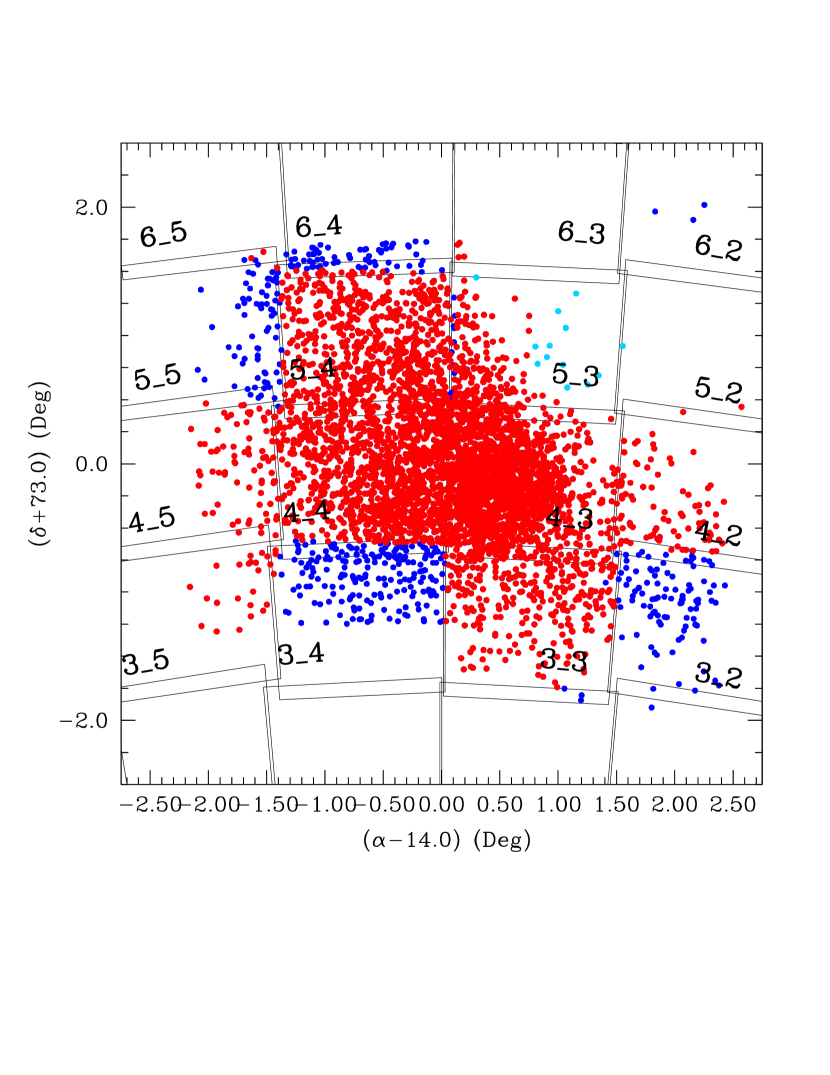
In this paper we present results for the CCs included in 11 tiles (each tile is 1.5 deg2 on the sky) completely or nearly completely observed, processed, and catalogued by the VMC survey as of 2015 March 9 (including observations obtained until 2014 September), namely the tiles SMC 3_3, 3_5, 4_2, 4_3, 4_4, 4_5, 5_2, 5_3, 5_4, 6_3, and 6_5. Figure 1 shows the spatial extent of the VMC tiles across the SMC body. The completed tiles do not cover the entire area surveyed by OGLE III. However, given the high concentration of CCs in the central body of the SMC, the number of pulsators included in the completed VMC tiles is about 90% of the total OGLE III sample. Table 1 lists the coordinates of the quoted tiles, as well as the number of CCs included in each tile.
In total, we were able to study 4159 objects of the 4630 OGLE III sample. To this number we have to add the 13 CCs from the EROS 2 data, leaving us with a final sample of 4172 CCs. The classification of the investigated pulsators in terms of Fundamental (F), First Overtone (FO), Second Overtone (SO), and mixed modes (F/FO, FO/SO, F/FO/SO, FO/SO/TO, where TO stands for Third Overtone) is shown in Table 2.
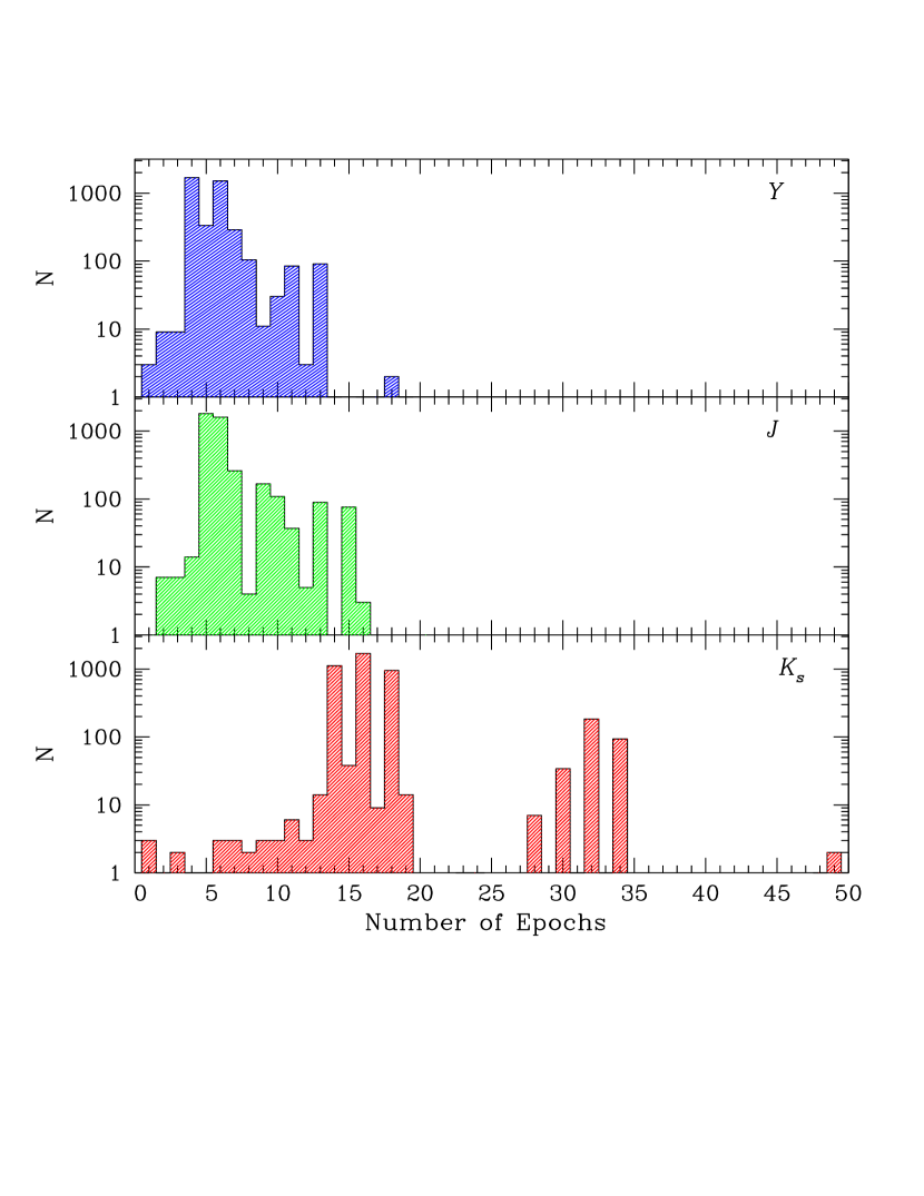


A general description of the observing strategy of the VMC survey can be found in Cioni et al. (2011). The procedures adopted to study the variable stars were discussed in detail by Ripepi et al. (2012a, b); Moretti et al. (2014); Ripepi et al. (2014b, 2015). However, it is worth recalling that the VMC -band time-series observations were scheduled to span 13 separate epochs distributed over several consecutive months. This observing strategy permits one to achieve well-sampled light curves for different types of variable stars, including RR Lyrae variables and Cepheids of all types. As for the and bands, the nominal number of epochs is four (two of these epochs are obtained with half exposure time) and may be acquired during the same night given that monitoring in these filters was not planned. However, a few additional epochs are usually available for each tile (especially in the -band), because some observing blocks (OBs) were executed outside of our specifications (typically for seeing values exceeding 0.8–1.0 arcsec), but the data were still useful since the CCs are relatively bright. In addition, there is a small overlap between the tiles. Consequently, the CCs present in multiple tiles possess at least twice the scheduled number of epochs. Given the high concentration of CCs in the contiguous tiles SMC 4_3, 4_4, 5_3, and 5_4 (see Fig. 1), we have more than 320 CCs whose light curves contain more than 28 phase points. This is also shown in the bottom panel of Fig. 2, where the bimodal distribution of epochs in the band is clear. From the figure, note that there are a few dozen stars with fewer than 13 epochs in . This can happen when the sources are located in underexposed areas and/or are affected by bright neighbours or bad pixels. We were still able to analyze these stars thanks to our template-fitting procedure (see Section 5).
The same considerations hold for the and bands, whose epoch distributions are shown in the top and middle panels of Fig. 2, respectively. In this case, the number of CCs with more than 10 epochs is 213 and 321 in the and bands, respectively. Similarly, the number of CCs with more than five epochs is 2121 and 2343 in and , respectively.
The VMC data were processed with the pipeline (Irwin et al., 2004) of the VISTA Data Flow System (VDFS, Emerson et al., 2004) and the photometry is in the VISTA photometric system (Vegamag=0). The time-series data analyzed in this work were downloaded from the VISTA Science Archive444http://horus.roe.ac.uk/vsa/ (VSA, Cross et al., 2012). Details about the data reduction can be found in the aforementioned papers. However, we briefly recall that (i) the pipeline applies a correction to the photometry of stars close to the saturation limit (Irwin, 2009). This task is very useful, because long-period CCs are very bright (–13) mag. The time-series photometry of these variables takes advantage of the VDFS capability to deal with the images for saturation, although the corrections applied do not always guarantee a full recovery of the data. (ii) The VSA processing produces quality flags for each star that are valuable to understand if the images have problems. This information is important for the following analysis.
To obtain the , , and light curves, the OGLE III (and EROS 2) catalog(s) of CCs described above were cross-correlated against the VMC catalog, taking all counterparts from the OGLE III and EROS 2 positions, regardless of their separation on the sky. About 95% of the objects have positions in agreement with those measured by OGLE III and EROS 2 within less than 0.1′′. Among the remaining 186 stars, 67 have a separation larger than 0.5′′ and are likely misidentifications. We will come back to these objects below.
III. Template-fitting procedure
Given the large number of light curves to analyze, it was convenient to find an automatic way to process the data. Our aim is to obtain an analytical or empirical model light curve that fits the observed one. This model can subsequently be used to measure the mean magnitude and the peak-to-peak amplitude for each variable. The usual way to carry out such a task is to use truncated Fourier series, adding as many harmonics as needed to obtain a good fit to the data (Schaltenbrand & Tammann, 1971). However, this kind of approach would not be useful in our case, because the presence of significant gaps in the light curve would lead to strong and unrealistic oscillations in the Fourier series.
Hence, we decided to use template light curves to fit the data. Following the pioneering work by Freedman (1988), templates to fit CC light curves based on only a few epochs in the NIR bands have already been presented and used by Soszyński et al. (2005); Inno et al. (2013, 2015). The typical approach in these studies consists of the following steps: (1) adopting templates constructed based on well-sampled CC ,, and light curves (Galactic or MC objects); (2) scaling the template amplitude using fixed amplitude ratios (e.g., A()/A(), with some dependence on period); (3) adopting literature period and epoch of maximum light to phase-match the template and the observed data. This technique is valuable, since it allows one to obtain an estimate of the average magnitude of a CC based on just one or two observed phase points. At the same time, given the uncertainties on the amplitude ratios and on the ephemerides, these estimates can easily be affected by errors as large as 5% (see also Sect. 3.3), despite the quite low amplitudes of the light curves in the NIR bands.
Our approach is fundamentally different from that outlined above (e.g., by Inno et al., 2013). Indeed, the availability of an average of 5.7, 6.3, and 16.7 phase points in , , and , respectively, allows us to safely rescale our templates in amplitude and phase match them using our observations directly. This procedure eliminates most of the uncertainties of the “classical” template method, because we do not have to rely on any fixed amplitude ratio to scale the templates in amplitude, nor do we have to use the literature epoch of maximum as reference to phase match the template and the observed data.

III.1. Template construction
The first step of our procedure was the construction of the templates. To this end, we visually inspected a large number of light curves, trying to select those with the most often recurring shapes, and at the same time, those exhibiting precise light curves. Particular care was devoted to covering a broad range of periods. This search was rather simple in , since in this band we have dozens of well-sampled and precise light curves for any period. However, we had fewer choices in and , given the much smaller number of well-sampled light curves in those filters.
At the end of this process, we concluded that a set of eight different templates for each band could reproduce the variety of shapes exhibited by the observed light curves.
Our templates were constructed as truncated Fourier series of the form
| (1) |
where is the magnitude, are the phases of the template light curves, is the zero point, which is zero by definition, is the number of terms of the series, and and are the amplitudes and phases of each term of the series, respectively. The first step consisted of fitting the selected observed light curves with splines in order to have smooth, densely sampled curves to be passed to the Fourier-series fitting program. This was needed to avoid spurious oscillations in the Fourier-series fit due to possible small gaps or undersampling at maximum/minimum of the light curves. This way, we actually constructed six of the eight different templates adopted for each filter. They are listed in Table 4, from T3 to T8. As for the two remaining templates, T1 simply consists of a pure cosine function for all filters (which is why the T1 template is not included in the table), while T2 reproduces a smooth curve which can often be observed in all of the , and bands for a broad range of periods (see T2 in Table 4). The shapes of the eight templates in all three filters are shown in Fig. 4.
III.2. Template fitting
The template-fitting procedure includes the following steps:
-
•
Scaling the templates with amplitude ratios, e.g., A()/A(), where we take A() from the OGLE III survey and the coefficients of these ratios from Soszyński et al. (2005). Similarly, the template is phase-matched with the observations using the ephemerides from OGLE III. The purpose of this step is only to provide a first-guess average magnitude for the target star and, in turn, to remove the most obvious outliers. In practice, we simply estimate the template values at the phases of the observed point and calculate the average difference between observed and calculated values, which is the approximate mean magnitude of the star.
-
•
Recalculating the template by varying its initial phase to find the phase shift that minimizes (by means of a least-squares fit) the difference data–template. This step provides an improved average magnitude (of the order of a few hundredths of mag).
-
•
Recalculating the template by varying its amplitude to find the amplitude scaling that minimizes (by means of a least-squares fit) the difference data–template. This step provides a further improvement of the average magnitude (again, a few hundredths of mag).
-
•
Fine-tuning outlier removal (at 2 and 3 levels in and in , respectively; the difference is because in we have many fewer phase points than in and, hence, we can simply remove obvious outliers) and final average-magnitude calculation (in intensity).
This procedure is applied to each template (in each band). Next, we need a tool to choose the template that optimally represents the data. After several trials and visual inspections of the resulting fits, we devised two main useful diagnostics. The first is the usual minimization, defined as
| (2) |
where is the total number of phase points, and are the magnitudes of the observed and computed light curves, respectively, and is the magnitude uncertainty per phase point.
The second criterion was devised empirically to take into account the fact that the smallest residuals can result from application of the wrong template simply because the outlier-removal process is too aggressive. Thus, we designed a Goodness (or G) parameter, defined as
| (3) |
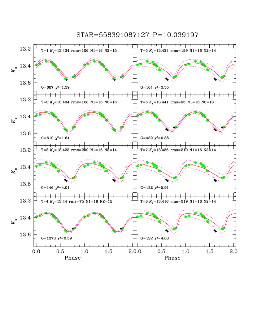
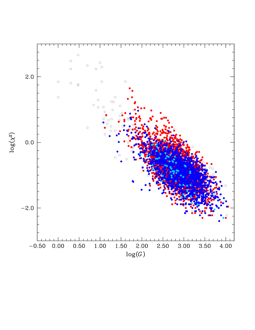
where is the r.m.s. of the fit and and are the numbers of phase points used in the fit and the total number of phase points, respectively. By definition, the first factor of tends to favor templates that give the smallest r.m.s. values, while the second factor favors those that remove the lowest number of outliers. The balance of these two features yields, in general, an automatic decision about the best templates that is in agreement with visual inspection of the fitting procedure. The value of can be used not only to choose the best template, but also as a more general indicator of the quality of the data and of the relative fitting procedure. Indeed, in general high values of (in our case, typically ) mean good data (and good fits), while lower values usually indicate significant scatter in the light curves. Extremely high values of (i.e., ) are also rather suspect because non-variable stars, exhibiting completely flat light curves (which happens, for example, when non-variable stars are considered owing to a coordinate missmatch with OGLE III Cepheid data) are expected to yield extremely high values of . Not surprisingly, the parameter is anti-correlated with the corresponding value: the higher is, the lower the becomes. An example of our template-fitting procedure can be found in Fig. 5 (note that in this case the best template is T4), while the anti-correlation between and is shown in Fig. 6.
III.3. Monte Carlo simulations
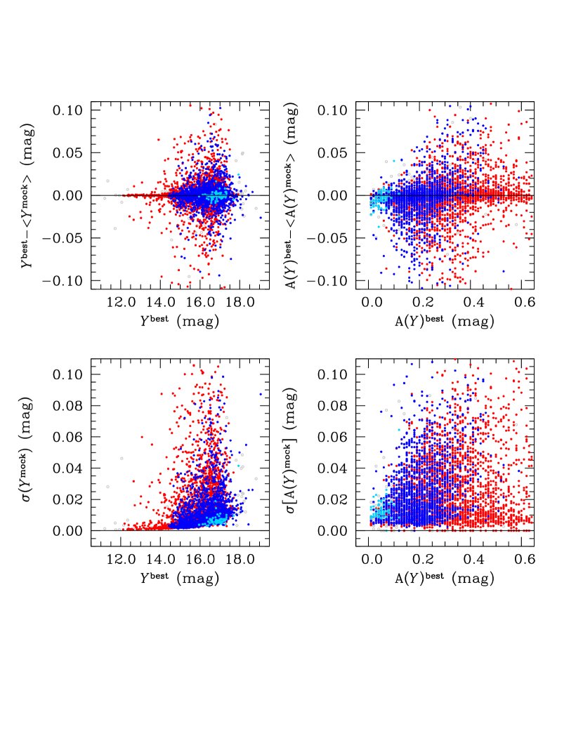
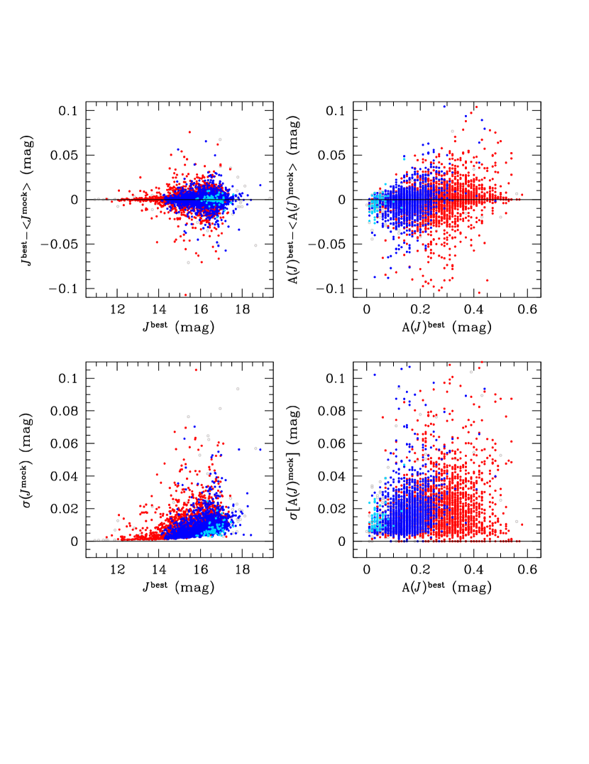
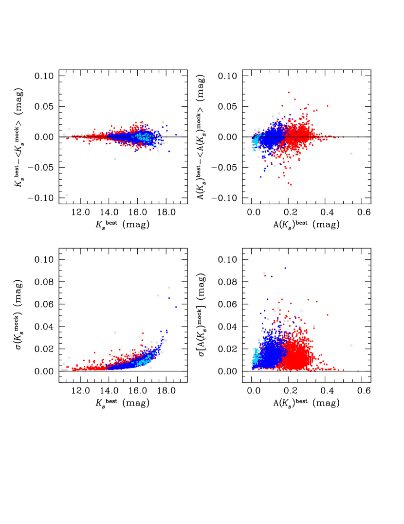
As an additional check of the reliability of the template-fitting procedure, and to estimate in a more quantitative way the precision achieved, we decided to use extensive Monte Carlo simulations. In practice, for each star (and for each filter), 100 different mock time series were created on the basis of the observed data, to which Gaussian noise was added with ’s corresponding to the average uncertainty on the phase points for the star of interest (different ’s were calculated for different filters). The template-fitting procedure outlined above was hence repeated 100 times and the average magnitude and r.m.s. were calculated. We then compared these quantities with those calculated from the observed data. The results of this exercise are summarized in Figs 7, 8, and 9. The top left-hand panels in each figure show the difference between the magnitude obtained with the best-fitting template () applied to the actual data and that resulting from averaging over the 100 mock light curves (). Similarly, the bottom left-hand panels show the r.m.s. of as a function of . These figures testify to the high precision reached in the band, where 84% and 99% of the stars have errors on the intensity-averaged magnitudes of mag and mag respectively. Only 1% and 0.1% of the CCs analyzed here have uncertainties mag and mag, respectively. The results are less favorable in the band and even worse in . In fact, in these bands the corresponding percentages drop to (68%, 93%, 7%, and 0.8%) and (56%, 78%, 22%, and 5.5%) in the and bands, respectively. The worse results in are mainly due to the fact that (a) the peak-to-peak amplitude in this filter is significantly larger than that in the band (consequently, it is more difficult to estimate the average magnitudes from undersampled light curves) and (b) we have, on average, fewer phase points in than in (5.6 versus 6.3).
The top and bottom right-hand panels in Figs 7, 8, and 9 display essentially the same results as the panels on the left, but for the peak-to-peak amplitudes instead of the intensity-averaged magnitudes. Again, the results for the amplitudes in the band are very good, while the uncertainties become significantly larger for the and, especially, the filters.
On the basis of the Monte Carlo experiments, we decided to assign as uncertainties to the intensity-averaged magnitudes and peak-to-peak amplitudes the values shown in the bottom panels of Figs 7, 8, and 9.
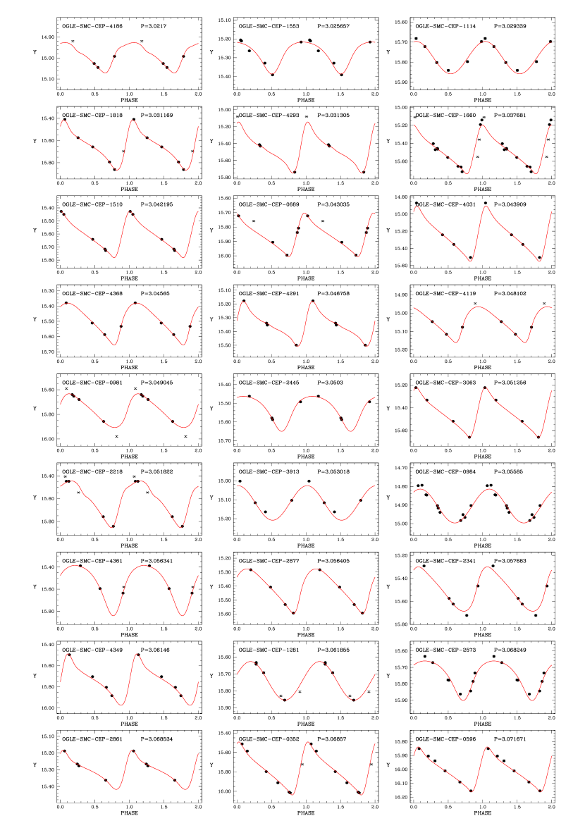
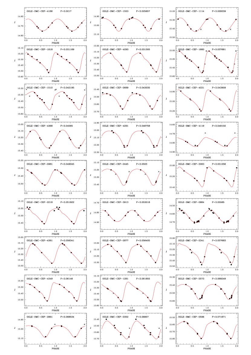
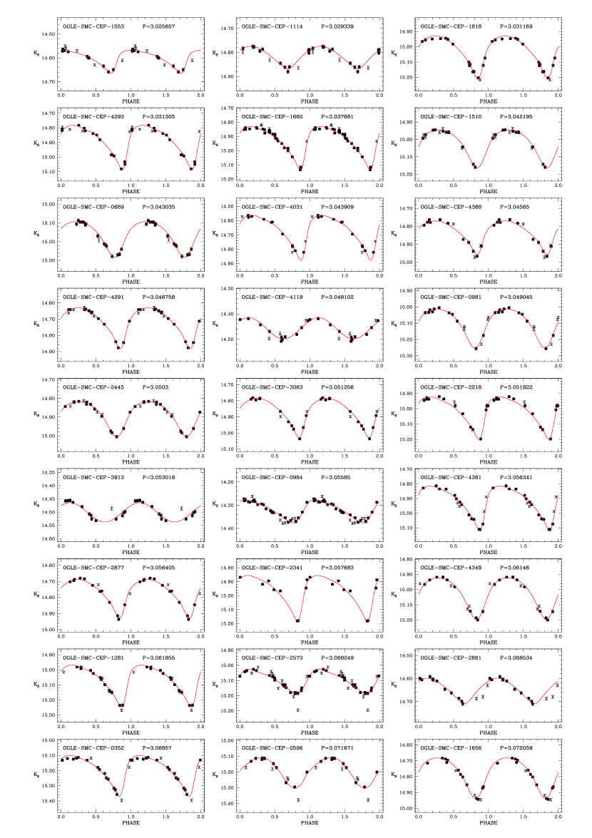
The light curves and the best-fitting templates found with the procedure outlined in this section are reported in Figs 10, 11, and 12 for the , and bands, respectively. These figures display the data for a subsample of 27 CCs; figures including the full data set of 4172 objects are available in the electronic version of this paper on the journal’s website.

Similarly, Table 5 reports the main physical quantities derived on the basis of the fitting procedure, namely the intensity-averaged magnitude for each variable (and each filter), the peak-to-peak amplitudes, and the relative errors calculated by means of the Monte Carlo experiments.
Finally, we recall that the , , and photometry described in this work is defined in the VISTA system. It is possible to compare our data with measurements in the widely used 2MASS system (Two Micron All Sky Survey Skrutskie et al., 2006) after applying the system transformations made available by the Cambridge Astronomy Survey Unit (CASU)555http://casu.ast.cam.ac.uk/surveys-projects/vista/technical/photometric-properties: ()2M=1.081(-)V, 2M=V+0.07(-)V, and 2M=V0.011(-)V. No transformation is provided in since 2MASS did not observe in this filter. However, it is possible to “standardize” the band by applying a color equation that, at present, is available only as a function of the color (and is therefore of no use to us). A new transformation using the () bands is being derived by CASU and will be available within a few months.
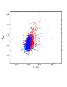
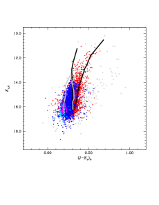
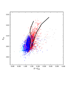
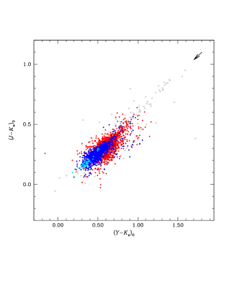
Since the intrinsic colors of the CCs investigated here typically range from 0.1 mag to 0.6 mag, the VISTA and 2MASS can be considered equivalent for CCs (see Fig. 13) to a very good approximation (better than 5 mmag), although the corrections needed in the band can be significant.
IV. Average magnitudes, colors and peak-to-peak amplitudes
We constructed color–magnitude diagrams for the entire sample of CC analyzed here, distinguishing them by the different types of pulsation. The results are shown in Fig. 13. The middle and right-hand panels of this figure display the comparison in the and planes of the observed data with the theoretical instability strips for F, FO, and SO CCs. The models, calculated for and , have been taken from Bono et al. (2000, 2001a, 2001b). We note that the models are in the Johnson system. Thus, we have to converted them into the VISTA system, adopting the VISTA–2MASS relations referred to in the previous section, as well as the color transformations available from Bessell & Brett (1988) and Carpenter (2001). As a result, we obtained the following approximate equations:
| (4) | |||||
| (5) | |||||
| (6) |
where the superscripts “V” and “J” refer to quantities in the VISTA and Johnson systems, respectively. There is general good agreement between predicted colors and observations, especially for FO pulsators, while for F pulsators the observed instability strip appears to be larger at low luminosities (i.e., short periods) compared with the predictions.
Additional information can be obtained from the color–color diagrams shown in Fig. 14, where the left- and right-hand panels show the and planes, respectively. In both cases, arrows represent the reddening vectors, which are almost parallel to the data distribution, making it almost impossible to use these planes to estimate individual reddening values. It is interesting to note the distribution of the rejected stars (empty gray circles), which is markedly elongated towards red colors (especially in the plane). This suggests significant contamination in the band by very red objects, likely red clump or red/asymptotic giant-branch stars, or bright (early-type) background galaxies. The right-hand panel of Fig. 14 shows the theoretical instability strip, now visible as an almost straight line passing, as expected, through the middle of the data distribution. Indeed, at fixed effective temperature, the position in the color–color plane is unequivocally determined by the adopted effective temperature–color transformation. Note that the modest broadening of the data (0.07-0.1 mag) is due to different contributions, namely the photometric errors, blending effects, and/or small metallicity differences, but not to reddening effects (see the direction of the reddening vectors in both planes of Fig. 14).
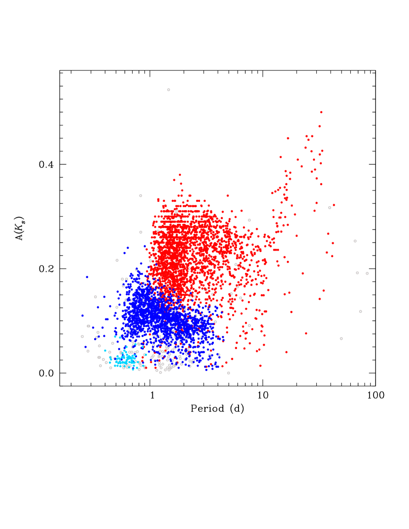
Figure 15 shows the period versus peak-to-peak amplitude in the band for the target CCs. As far as we know, this is the first time that such a plane has been exploited with such a statistically significant number of objects in an infrared band. An inspection of the figure reveals the clean separation in amplitude of the three different modes. It is interesting to note that the peculiar shape of the distribution of F pulsators, with an increase at about d and a maximum around –24 d, resembles a similar trend observed in the visual band for the Galactic CCs (Bono et al., 2000) and is consistent with theoretical predictions (see their Fig. 7).
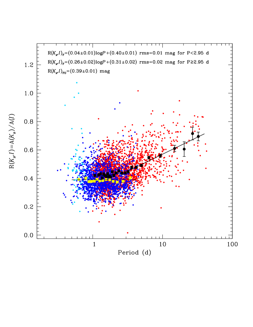
We also looked at the peak-to-peak amplitude ratios for different pulsation modes between the and bands. These values may be useful for authors who want to use the canonical template-fitting procedure. Figure 16 shows the ()= A()/A() ratio versus period for the CCs investigated here. We calculated the ratio between these bands, because our amplitudes are more accurate in relative to and (see Section 5) and OGLE III provides the peak-to-peak amplitudes for all Cepheids investigated here only in the filter.
Given the rather large scatter in the data (possibly in part due to the presence of binary companions), we decided to average the CCs in period bins, obtaining the light blue and yellow filled circles for F and FO pulsators, respectively (we did not consider the SO CCs because of their very small amplitudes). An analysis of the averaged data reveals the different behavior of F and FO pulsators. () is almost constant for FO pulsators over the full period range, while for F pulsators it is flat only until d. For longer periods there is a steep linear increase of () with period. Quantitatively, we derived the following equations for F and FO pulsators:
| (7) | |||||
| (8) | |||||
| (9) |
It is interesting to note that the steep change in slope for F pulsators occurs at about the same period where we find a break in the , , and relations (see next section).
A comparison of our results with those in the literature reveals some differences. Indeed, concerning F pulsators only, Soszyński et al. (2005) suggest using constant values of =0.49 or 0.62 for periods / 20 d, respectively. Using Eq. 8, for d we obtain =0.65, which is fully compatible with Soszyński et al. (2005)’s values. However, it is easy to verify that the agreement is worse for different periods. For example, at d, we obtain =0.73, while at d =0.41. Taking into account that the Soszyński et al. (2005) results have been derived using Galactic and LMC CCs, it is reasonable to hypothesize that part of the discrepancy between our and their findings can be owing to the different metallicities of the adopted CC samples.
We cannot perform a direct comparison with Inno et al. (2015)’s results, because they only provide the ratio of NIR bands with respect to the band. However, we can compare the trends versus the periods, since they have different data sets for Galactic+LMC and SMC CCs. As a result, Inno et al. (2015) found a break in at a period similar to that of Soszyński et al. (2005). This is in contrast with our results (perhaps this is due to the smaller size of their sample). On the other hand, they found systematically lower values for SMC CCs, with respect to the Galactic+LMC variables, in full agreement with our results.
V. , , and relations
The data reported in Table 5 allow us to derive several useful relationships, adopting various combinations of magnitudes and colors. In particular, we derived relations in , , and , as well as and relations for the following combinations: (,), (,), and (,).
Before deriving the latter relationships we have to take account of the reddening. We adopted the extinction maps of Haschke, Grebel & Duffau (2011), as we already successfully did in our previous papers (see, e.g., the discussion in Sect. 3 of Ripepi et al., 2015). The reddening values were converted using the following equations: ()=1.80(); ()=2.24(); ()=0.43() (Cardelli et al., 1989; Kerber et al., 2009; Gao et al., 2013).666The coefficients used in this paper are consistent with the 2MASS system, to which the VISTA system is related. The coefficients of the relations were calculated in a similar fashion.
To derive the relevant relationships for F, FO, and SO variables, we adopted equations of the form , , and for the , , and relations, respectively. Here, and represent two different magnitudes from among , , , and . The details about the combinations of magnitudes and colors adopted in this papers can be found in Table 6. In order to use the full sample of pulsators, including the double- or multi-mode CCs, we decided to use them with the period of the dominant mode (e.g., F-mode if the star is an F/FO double-mode pulsator, and so on). This procedure is safe, since from our previous investigation of LMC pulsators (Ripepi et al., 2012a) we know that these objects do not exhibit systematic luminosity differences with respect to single-mode objects.
The next step involved checking for the presence of changes in the slope of the different relationships, as found in previous studies in the literature (see, e.g. Subramanian & Subramaniam, 2015, and references therein). To this aim, we used the in which was known from our previous investigation of the LMC CCs, to show a small intrinsic dispersion (see, e.g. Ripepi et al., 2012a), and which is thus particularly appropriate for our purpose. As a result, we found that there is a clear change in slope at ( 2.95 d) for F-mode pulsators, while there is no significant change in slope for FO variables. This was confirmed by the analysis of the and in different filters and is in agreement with the results obtained in the optical ( bands) for the OGLE III sample of F-mode pulsators by Subramanian & Subramaniam (2015) (see also references in this paper). However, we do not find the break at ( 1.07 d) that they noticed for FO-mode pulsators. A possible explanation for the break detected at 3 d is that for shorter periods the blue loop of the Cepheid evolutionary track is too short and enters only the reddest part of the instability strip (M. Marconi et al., in prep).
The was also used to analyze problematic objects, identified as clear outliers from these relations. In total, we discarded 223 CCs. We identified different (but often concurrent) reasons for the erratic behavior of these objects (see the final column in Table 5 for details): (i) misidentification: all objects with separation VMC–OGLE III 0.2′′ were visually inspected and rejected if they were found to be overluminous in the relation (more than 100 objects were rejected as such); (ii) scattered or heavily undersampled light curves (always low /high values; more than 50 such objects were present); (iii) notes from either OGLE III or VMC, i.e., the presence of flags reporting problems with the images (more than 20 rejections); (iv) saturation (seven objects). Note also that 17 objects with good VMC photometry were rejected because they lacked OGLE III -band photometry. Not all outliers can be explained by invoking these reasons; in fact, there are 35 outliers for which we could find no apparent flaws. However, most are faint and all are overluminous. Hence, it is likely that they suffer from blending with bright neighbor stars. The discarded stars are reported separately, both in Table 5 and Figs 10, 11, and 12. Finally, we note that a few other objects were excluded from the derivation of the , , and relations involving the or bands because of specific problems in these bands. To avoid confusion, these objects have not been highlighted in the table and figures.
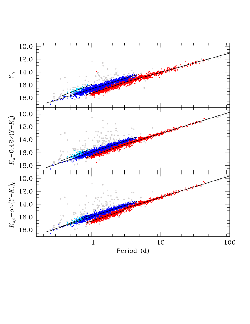
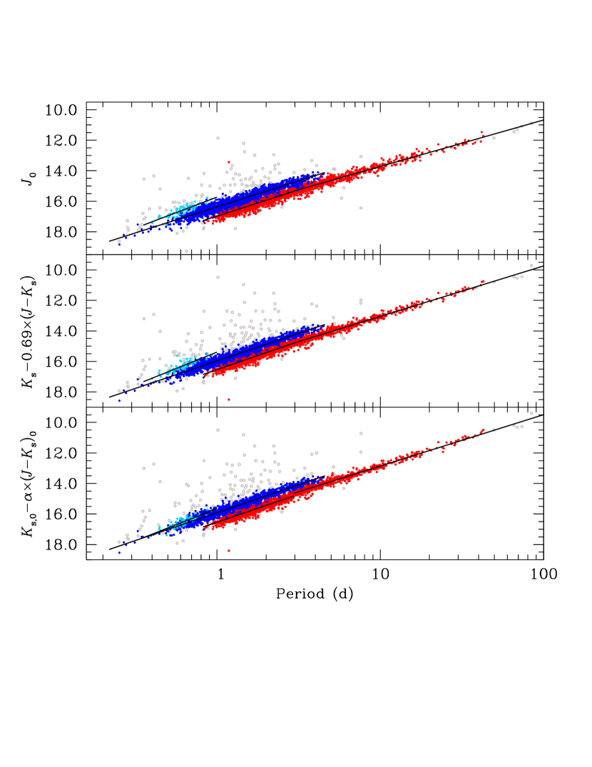
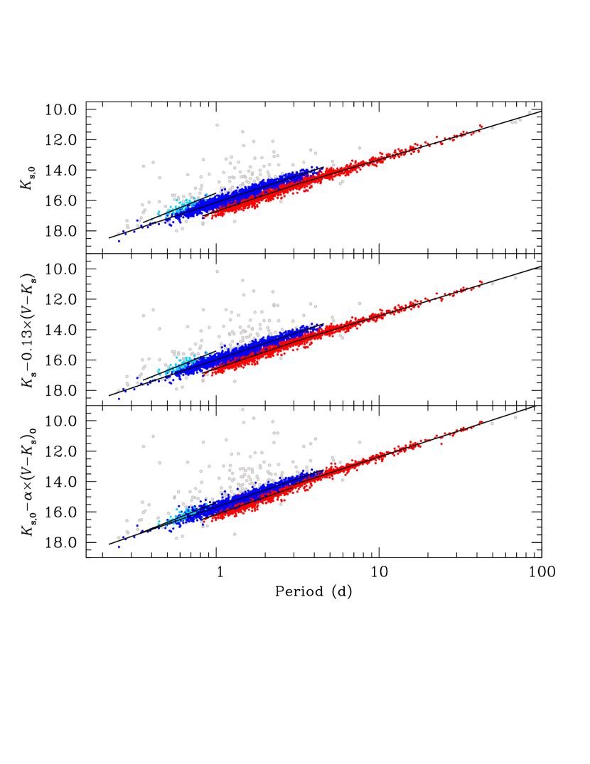
On this basis, we performed a least-squares fit to the data to derive all relations, adopting a break at (2.95 d) for F-mode CCs, while all FO- and SO-mode pulsators were used together. The results of this work are shown in Table 6 and Figs 17, 18, and 19, where from top to bottom we display the F-, FO-, and SO-mode , , and relations, respectively. Note that the relations show a distinct discontinuity at owing to the way the data are projected in two dimensions. As far as we know, these are the first CC , , and relations ever derived that involve the band. The same is true for SO pulsators, even if in this case the small number of objects available for the calculations (about 70) and their intrinsic faintness did not allow us to obtain , , and relations to similar precision as those for F and FO pulsators (see Table 6).
The regressions listed in Table 6 (and in Figs 17, 18, and 19) show that the relations have, as expected, a larger dispersion with respect to the and relations, which show a similar scatter for all combinations of magnitudes and colors, even though the use of and give slightly better results. This is not surprising, since the general quality of the -band data is (moderately) worse than that in . In any case, the constancy of the dispersion of all these relations is a clear indication that the elongated structure of the SMC is dominating the intrinsic dispersion of these relations, which we know from LMC studies to be much smaller (see, e.g. Ripepi et al., 2012a; Inno et al., 2013; Macri et al., 2015).
We can now compare our results with the previous investigation by Inno et al. (2013). These authors derived relations for a variety of combinations of magnitudes and colors for SMC and LMC CCs, including the NIR bands . Their photometric database relies mainly on single-epoch light curves, from which they derived average magnitudes by adopting some literature template light curves and relying on published ephemerides and amplitude ratios (e.g., A()/A()). It is important to note our very different approach with respect to theirs. Indeed, the larger number of observed epochs (especially in the band) allowed us to adopt a template procedure without having to rely on any external information (apart from the periods, see details in Section 5) and which is capable of achieving much higher precision of the intensity-averaged photometry for each individual CC. The relations we can compare with Inno et al. (2013) are the and for F and FO pulsators. The latter authors calculated these relations in different ways, either without taking into account any break or by arbitrarily imposing breaks at . Therefore, we can compare the and relations with no break for FO pulsators (Table 1 of Inno et al., 2013) and the relation for F pulsators with a break at (see Table 3 of Inno et al., 2013)777Note that Inno et al. (2013)’s relations are not provided for different breaks, nor do they have relations for . To take into account that our photometry is in the VISTA system, while Inno et al. (2013)’s were in the 2MASS system, we have applied the equations discussed in Section 5 to convert Inno et al. (2013)’s relations to the VISTA system. We can now finally perform the comparison with the values listed in our Table 6. We obtain very good agreement for the three relations quoted above, in all cases within . However, we emphasize that the precision for the individual CC magnitudes is better in our case given the larger number of observations. This is an important factor when dealing with the structure of the SMC, whose study requires precise individual relative distances.
V.1. The relative distance between SMC and LMC and the absolute distance of the SMC
The relationships derived in the previous Section will be used in a forthcoming paper to study in detail the 3D structure of the SMC. However, a first important use of the data presented in this paper is the estimation of the relative distance between the two MCs. In turn, the assumption of a distance for the LMC, which can be more safely determined with respect to the SMC’s (since the SMC is so significantly elongated), allows us to provide an estimate of the absolute distance to the SMC (or, rather, of the center defined by the CC distribution).
We hence proceeded using our own data published in Ripepi et al. (2012a) for the CCs in the LMC. This is justified because (i) we used data in the same photometric system, (ii) we obtained a relation with very low dispersion for the LMC CCs, and (iii) we also provided an absolute distance estimate for the LMC.
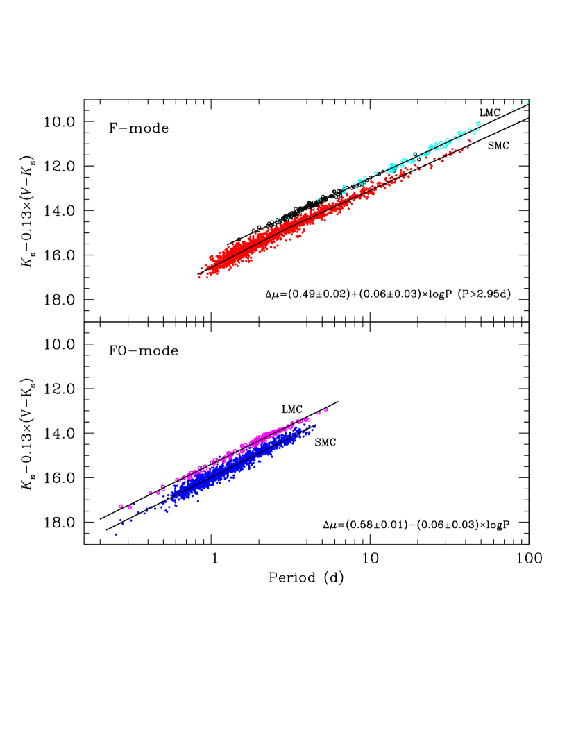
The technique adopted is illustrated in Fig. 20, where we compare the relations for F- and FO-mode pulsators (top and bottom panels, respectively). First, observing the period distribution of the CCs in the LMC and the fact that the slope of the LMC’s relation is very close to the slope we have found here for the SMC CCs characterized by , we used this latter relation for our comparison of F-mode pulsators. Nonetheless, the slopes of the relations for both F- and FO-mode pulsators are slightly different for the LMC and SMC (which is possibly related to a weak but significant metallicity dependence). Indeed, it is possible to describe the difference in , which translates directly into a difference in distance modulus as a function of period with two simple equations:
| (10) | |||||
| (11) |
where means the difference in distance modulus of SMC and LMC, and the errors take into account the uncertainties in both the LMC and SMC relations. To use Eq. 10 and 11, we have to fix pivoting periods to determine the values. After some tests we chose d and d for F- and FO-mode pulsators, respectively. These values are approximately in the middle of the period range for both pulsator types, but it is easy to verify that the results do not depend significantly on this choice. The result of this exercise gives: mag and mag, in excellent mutual agreement. Averaging the two results we obtain our best estimate for the relative distance between the MCs: mag. This value is in good agreement with that derived in a similar fashion by Inno et al. (2013), especially with their result for FO pulsators: mag, while for F-mode CCs they find mag. Our estimate is somewhat larger than those quotes in other papers based on different standard candles (see de Grijs et al., 2014, for a large compilation of distance differentials). For example, Cioni et al. (2000b) found from the tip of the red-giant branch, while using RR Lyrae stars Szewczyk et al. (2009) found a significantly smaller value, mag. According to Matsunaga et al. (2011), Type II Cepheids (W Vir) yield or mag (depending on the use of NIR or optical data, respectively). In general, Table 4 of Matsunaga et al. (2011), where they list several literature results, seems to suggest that all evaluations of the based on CCs provide larger values with respect to those based on population II indicators. This can be due to the very different spatial distribution among CCs (typically showing a disk-like location in both MCs) and population II tracers (e.g., RR Lyrae stars, type II Cepheids, which are more evenly distributed around a sort of spheroid in both MCs), as shown, e.g., by Deb & Singh (2014); Moretti et al. (2014); Deb et al. (2015).
The absolute distance to the SMC can be determined by simply adding to the estimated above the preferred absolute distance for the LMC. There are hundreds of such estimates in the literature (see de Grijs et al., 2014, for a thorough review), but here we will consider in particular two values: (1) mag obtained in our previous work on LMC CCs (Ripepi et al., 2012a), and (2) , accurately estimated by Pietrzyński et al. (2013) on the basis of an eclipsing Cepheid binary star. As a result, we obtain: (1) mag and (2) mag. These values are formally in agreement within with that obtained in de Grijs & Bono (2015) by averaging a large number of literature estimates: mag. However, as noted by these latter authors, the systematic uncertainty on this determination, caused by different sources (mainly the complex SMC geometry and its elongation along the line of sight), can be as large as 0.15–0.20 mag.
VI. Conclusions
In this paper we have presented the VMC survey’s light curves for 4172 CCs in the SMC. The majority of the objects have optical data as well as identification and periods from the OGLE III survey, while 13 CCs have been identified by the EROS 2 survey. Our data set consists of , , and light curves with the number of epochs typically ranging from 4 to 12 in and , and 13 to 36 in . We used our best light curves in each filter to construct samples of eight templates covering the full variety of periods and light-curve shapes. These templates have been used to automatically perform least-squares fits to the observations by varying both the amplitude and the phasing, and eventually choosing the best-fitting template by means of appropriately chosen parameters. We provide intensity-averaged magnitudes and peak-to-peak amplitudes in the , , and filters. To estimate reliable uncertainties on these values, we carried out Monte Carlo simulations, producing 100 mock light curves, adding Gaussian errors to the actual data for each CC in each filter, and running the template-fitting procedure from scratch each time. This process allowed us to assess the reliability of our template-fitting procedure and estimate robust uncertainties on CC magnitudes and amplitudes.
The intensity-averaged magnitudes in the VISTA , , and filters have been complemented with optical -band data and periods to construct a variety of , , and relations for the CCs in the SMC. The relations involving , , and are in agreement with those in the literature. As for the band, to our knowledge in this paper we present the first CC , , and ever obtained using this filter. The , , and relations in the , and bands for F- and FO-mode CCs in the SMC presented here are the most accurate to date, since they are based on well- or moderately well-sampled light curves in and , respectively. We also presented the first NIR , , and relations for SO pulsators to date.
We used the relation to estimate the relative SMC–LMC distance and, in turn, the absolute distance of the SMC. For the former, we derive mag, a value that is in rather good agreement with other evaluations based on CCs, but in disagreement (significantly larger) with estimates based on (old) population II distance indicators. We speculate that this discrepancy may be mainly due to the different geometric distribution of young and old tracers in the MCs. As for the absolute distance to the SMC, our best estimates, mag and mag, based on two particular evaluations of the distance to the LMC, are in good agreement with literature values. However, we have to take into account the large systematic uncertainty due to the complex geometry of the SMC. In a forthcoming paper, we will use our precise relations to unveil the 3D structure of the SMC. For the reasons outlined above, this work is also expected to reduce the systematic uncertainties associated with the absolute distance to the SMC.
References
- Bessell & Brett (1988) Bessell, M. S., & Brett, J. M. 1988, PASP, 100, 1134
- Bono et al. (1999) Bono, G., Caputo, F., Castellani, V., & Marconi, M. 1999, ApJ, 512, 711
- Bono et al. (2000) Bono, G., Castellani, V., & Marconi, M. 2000, ApJ, 529, 293
- Bono et al. (2001a) Bono, G., Caputo, F., & Marconi, M. 2001a, MNRAS, 325, 1353
- Bono et al. (2001b) Bono, G., Gieren, W. P., Marconi, M., & Fouqué, P. 2001b, ApJ, 552, L141
- Bono et al. (2010) Bono, G., Caputo, F., Marconi, M., & Musella, I. 2010, ApJ, 715, 277
- Caputo et al. (2000) Caputo, F., Marconi, M., & Musella, I. 2000, A&A, 354, 610
- Carpenter (2001) Carpenter, J. M. 2001, AJ, 121, 2851
- Cardelli et al. (1989) Cardelli, J. A., Clayton, G. C., & Mathis, J. S. 1989, ApJ, 345, 245
- Carini et al. (2014) Carini, R., Brocato, E., Marconi, M., & Raimondo, G. 2014, A&A, 561, A110
- Cioni et al. (2000a) Cioni, M.-R. L., Habing, H. J., & Israel, F. P. 2000a, A&A, 358, L9
- Cioni et al. (2000b) Cioni, M.-R. L., van der Marel, R. P., Loup, C., & Habing, H. J. 2000b, A&A, 359, 601
- Cioni et al. (2011) Cioni, M.-R. L., Clementini, G., Girardi, L., et al. 2011, A&A, 527, A116
- Cross et al. (2012) Cross, N. J. G., et al. 2012, A&A, 548, A119
- Dalton et al. (2006) Dalton, G. B., Caldwell, M., Ward, A. K., et al. 2006, Proc. SPIE, 6269, 62690X
- Deb et al. (2015) Deb, S., Singh, H. P., Kumar, S., & Kanbur, S. M. 2015, MNRAS, 449, 2768
- Deb & Singh (2014) Deb, S., & Singh, H. P. 2014, MNRAS, 438, 2440
- Fiorentino et al. (2013) Fiorentino, G., Musella, I., & Marconi, M. 2013, MNRAS, 434, 2866
- de Grijs et al. (2014) de Grijs, R., Wicker, J. E., & Bono, G. 2014, AJ, 147, 122
- de Grijs & Bono (2015) de Grijs, R., & Bono, G. 2015, AJ, 149, 179
- Deb et al. (2015) Deb, S., Singh, H. P., Kumar, S., & Kanbur, S. M. 2015, MNRAS, 449, 2768
- Dobbie et al. (2014) Dobbie, P. D., Cole, A. A., Subramaniam, A., & Keller, S. 2014, MNRAS, 442, 1663
- Emerson et al. (2004) Emerson J. P., Irwin M. J., Lewis J., et al., 2004, Proc. SPIE, 5493, 401, 41
- Emerson et al. (2006) Emerson, J., McPherson, A., & Sutherland, W. 2006, The Messenger, 126, 41
- Fiorentino et al. (2002) Fiorentino, G., Caputo, F., Marconi, M., & Musella, I. 2002, ApJ, 576, 402
- Freedman (1988) Freedman, W. L. 1988, ApJ, 326, 691
- Freedman et al. (2001) Freedman, W. L., Madore, B. F., Gibson, B. K., et al. 2001, ApJ, 553, 47
- Freedman & Madore (2011) Freedman W. L., Madore B. F., 2011, ApJ, 734, 46
- Gao et al. (2013) Gao, J., Jiang, B. W., Li, A., & Xue, M. Y. 2013, ApJ, 776, 7
- Glatt et al. (2008) Glatt, K., Grebel, E. K., Sabbi, E., et al. 2008, AJ, 136, 1703
- Hammer et al. (2015) Hammer, F., Yang, Y. B., Flores, H., Puech, M., & Fouquet, S. 2015, ApJ, 813, 110
- Harris (2007) Harris, 2007, ApJ, 658, 345
- Harris & Zaritsky (2004) Harris J., Zaritsky D., 2004, AJ, 127, 1531
- Harris & Zaritsky (2009) Harris J., Zaritsky, D., 2009, AJ, 138, 1243
- Haschke, Grebel & Duffau (2011) Haschke R., Grebel E. K., Duffau, S., 2011, AJ, 141, 158
- Haschke et al. (2012) Haschke, R., Grebel, E. K., & Duffau, S. 2012, AJ, 144, 107
- Hatzidimitriou & Hawkins (1989) Hatzidimitriou, D., & Hawkins, M. R. S. 1989, MNRAS, 241, 667
- Inno et al. (2013) Inno, L., Matsunaga, N., Bono, G., et al. 2013, ApJ, 764, 84
- Inno et al. (2015) Inno, L., Matsunaga, N., Romaniello, M., et al. 2015, A&A, 576, A30
- Irwin et al. (1985) Irwin, M. J., Kunkel, W. E., & Demers, S. 1985, Nature, 318, 160
- Irwin et al. (2004) Irwin M. J., Lewis J., Hodgkin S., et al., 2004, Proc. SPIE, 5493, 411
- Irwin (2009) Irwin, M. J. 2009, UKIRT Newsletter, 25, 15
- Kerber et al. (2009) Kerber L. O., Girardi L., Rubele S., Cioni M.-R., 2009, A&A, 499, 697
- Kim et al. (2014) Kim, D.-W., Protopapas, P., Bailer-Jones, C. A. L., et al. 2014, A&A, 566, A43
- Macri et al. (2015) Macri, L. M., Ngeow, C.-C., Kanbur, S. M., Mahzooni, S., & Smitka, M. T. 2015, AJ, 149, 117
- Madore (1982) Madore, B. F. 1982, ApJ, 253, 575
- Marconi et al. (2004) Marconi, M., Fiorentino, G., & Caputo, F. 2004, A&A, 417, 1101
- Marconi et al. (2005) Marconi, M., Musella, I., & Fiorentino, G. 2005, ApJ, 632, 590
- Marconi (2009) Marconi, M. 2009, Mem. Soc. Astron. Italiana, 80, 141
- Marconi et al. (2010) Marconi, M., Musella, I., Fiorentino, G., et al. 2010, ApJ, 713, 615
- Matsunaga et al. (2011) Matsunaga, N., Feast, M. W., & Soszyński, I. 2011, MNRAS, 413, 223
- Moretti et al. (2014) Moretti, M. I., Clementini, G., Muraveva, T., et al. 2014, MNRAS, 437, 2702
- Muraveva et al. (2015) Muraveva, T., Palmer, M., Clementini, G., et al. 2015, ApJ, 807, 127
- Nidever et al. (2013) Nidever, D. L., Monachesi, A., Bell, E. F., et al. 2013, ApJ, 779, 145
- Ngeow et al. (2008) Ngeow, C., Kanbur, S. M., & Nanthakumar, A. 2008, A&A, 477, 621
- Persson et al. (2004) Persson S. E., Madore B. F., Krzemiński W., et al., 2004, AJ, 128, 2239
- Piatti et al. (2015) Piatti, A. E., de Grijs, R., Rubele, S., et al. 2015, MNRAS, 450, 552
- Pietrzyński et al. (2013) Pietrzyński, G., Graczyk, D., Gieren, W., et al. 2013, Nature, 495, 76
- Putman et al. (1998) Putman, M. E., Gibson, B. K., Staveley-Smith, L., et al. 1998, Nature, 394, 752
- Riess et al. (2011) Riess, A. G., Macri, L., Casertano, S., et al. 2011, ApJ, 730, 119
- Ripepi et al. (2012a) Ripepi, V., Moretti, M. I., Marconi, M., et al. 2012a, MNRAS, 424, 1807
- Ripepi et al. (2012b) Ripepi, V., Moretti, M. I., Clementini, G., et al. 2012b, Ap&SS, 341, 51
- Ripepi et al. (2014a) Ripepi, V., Cignoni, M., Tosi, M., et al. 2014, MNRAS, 442, 1897
- Ripepi et al. (2014b) Ripepi, V., Marconi, M., Moretti, M. I., et al. 2014, MNRAS, 437, 2307
- Ripepi et al. (2015) Ripepi, V., Moretti, M. I., Marconi, M., et al. 2015, MNRAS, 446, 3034
- Romaniello et al. (2008) Romaniello, M., Primas, F., Mottini, M., et al. 2008, A&A, 488, 731
- Rubele et al. (2015) Rubele, S., Girardi, L., Kerber, L., et al. 2015, MNRAS, 449, 639
- Scowcroft et al. (2016) Scowcroft, V., Freedman, W. L., Madore, B. F., et al. 2016, ApJ, 816, 49
- Shapley (1940) Shapley H., 1940, Bull. Harvard Coll. Obs., 914, 8
- Schaltenbrand & Tammann (1971) Schaltenbrand, R., & Tammann, G. A. 1971, A&AS, 4, 265
- Skrutskie et al. (2006) Skrutskie, M. F., Cutri, R. M., Stiening, R., et al. 2006, AJ, 131, 1163
- Soszyński et al. (2005) Soszyński, I., Gieren, W., & Pietrzyński, G. 2005, PASP, 117, 823
- Soszyński et al. (2010) Soszyński, I., Poleski, R., Udalski, A., et al. 2010, Acta Astronomica, 60, 17
- Stanimirović et al. (2004) Stanimirović, S., Staveley-Smith, L., & Jones, P. A. 2004, ApJ, 604, 176
- Subramanian & Subramaniam (2015) Subramanian, S., & Subramaniam, A. 2015, A&A, 573, A135
- Szewczyk et al. (2009) Szewczyk, O., Pietrzyński, G., Gieren, W., et al. 2009, AJ, 138, 1661
- Tisserand et al. (2007) Tisserand, P., Le Guillou, L., Afonso, C., et al. 2007, A&A, 469, 387
- Udalski et al. (1999) Udalski, A., Szymanski, M., Kubiak, M., et al. 1999, Acta Astronomica, 49, 201
- Welch et al. (1987) Welch, D. L., McLaren, R. A., Madore, B. F., & McAlary, C. W. 1987, ApJ, 321, 162
- Westerlund (1997) Westerlund B. E., 1997, The Magellanic Clouds. CUP, Cambridge
- Zaritsky et al. (2000) Zaritsky, D., Harris, J., Grebel, E. K., & Thompson, I. B. 2000, ApJ, 534, L53
| Tile | RA | DEC | N |
|---|---|---|---|
| hh mm ss.sss | |||
| SMC 3_3 | 00 44 55.896 | 74 12 42.120 | 315 |
| SMC 3_5 | 01 27 30.816 | 74 00 49.320 | 25 |
| SMC 4_2 | 00 25 14.088 | 73 01 47.640 | 86 |
| SMC 4_3 | 00 45 14.688 | 73 07 11.280 | 1642 |
| SMC 4_4 | 01 05 19.272 | 73 05 15.360 | 1128 |
| SMC 4_5 | 01 25 11.088 | 72 56 02.760 | 83 |
| SMC 5_2 | 00 26 41.688 | 71 56 35.880 | 2 |
| SMC 5_3 | 00 45 32.232 | 72 01 40.080 | 197 |
| SMC 5_4 | 01 04 26.112 | 71 59 51.000 | 687 |
| SMC 6_3 | 00 45 48.792 | 70 56 09.240 | 4 |
| SMC 6_5 | 01 21 22.560 | 70 46 11.640 | 3 |
| F | FO | SO | F/FO | FO/SO | F/FO/SO | FO/SO/TO |
|---|---|---|---|---|---|---|
| 2377 | 1472 | 74 | 52 | 196 | 2 | 1 |
| 55492.59731 | 19.076 | 0.040 |
| 55492.63328 | 19.130 | 0.040 |
| 55497.70319 | 19.116 | 0.047 |
| 55539.61969 | 19.114 | 0.051 |
| 55493.58975 | 18.788 | 0.041 |
| 55493.62870 | 18.830 | 0.039 |
| 55495.55177 | 18.860 | 0.063 |
| 55539.64087 | 18.912 | 0.060 |
| 55778.75378 | 18.817 | 0.052 |
| 55493.78892 | 18.641 | 0.099 |
| 55495.57575 | 18.699 | 0.168 |
| 55495.68566 | 18.688 | 0.111 |
| 55497.72461 | 18.776 | 0.153 |
| 55538.62081 | 18.681 | 0.125 |
| 55549.58532 | 18.777 | 0.135 |
| 55769.75425 | 18.697 | 0.126 |
| 55778.77517 | 18.683 | 0.169 |
| 55791.76203 | 18.706 | 0.110 |
| 55818.73171 | 18.807 | 0.148 |
| 55820.67458 | 18.484 | 0.088 |
| 55879.55553 | 18.542 | 0.111 |
| 55880.61929 | 18.737 | 0.137 |
| 55900.57090 | 18.674 | 0.115 |
| 56130.79475 | 18.704 | 0.116 |
| 56173.70295 | 18.712 | 0.136 |
| 56195.64097 | 18.668 | 0.111 |
| 56223.54177 | 18.704 | 0.125 |
Note. — Table 3 is published in its entirety in the electronic edition of the Astrophysical Journal. A portion is shown here for guidance regarding its form and content.
| Parameter | T2 | T3 | T4 | T5 | T6 | T7 | T8 |
|---|---|---|---|---|---|---|---|
| –Band | |||||||
| 0.49260 | 0.12614 | 0.12888 | 0.20863 | 0.20097 | 0.17442 | 0.15502 | |
| 0.14500 | 0.03315 | 0.07549 | 0.11718 | 0.09804 | 0.05488 | 0.03855 | |
| 0.04100 | 0.01090 | 0.04152 | 0.05601 | 0.04747 | 0.02273 | 0.02314 | |
| 0.01000 | 0.00448 | 0.01609 | 0.02200 | 0.01831 | 0.01211 | 0.00984 | |
| 0.00000 | 0.00209 | 0.00580 | 0.00765 | 0.00370 | 0.00640 | 0.00483 | |
| 0.00000 | 0.00124 | 0.00000 | 0.00253 | 0.00190 | 0.00345 | 0.00146 | |
| 0.00000 | 0.00065 | 0.00000 | 0.00026 | 0.00276 | 0.00171 | 0.00078 | |
| 0.00000 | 0.00035 | 0.00000 | 0.00044 | 0.00173 | 0.00081 | 0.00054 | |
| 0.00000 | 0.00022 | 0.00000 | 0.00008 | 0.00054 | 0.00031 | 0.00041 | |
| 0.00000 | 0.00017 | 0.00000 | 0.00027 | 0.00024 | 0.00010 | 0.00022 | |
| 1.40800 | 5.75860 | 2.52701 | 1.50221 | 0.72710 | 5.27327 | 5.93367 | |
| 2.52800 | 3.65703 | 3.36472 | 1.50458 | 6.08919 | 3.02993 | 4.57391 | |
| 3.55200 | 1.23267 | 4.18291 | 1.34113 | 5.11517 | 1.14020 | 3.82891 | |
| 4.43800 | 5.38378 | 5.03844 | 0.97634 | 4.16420 | 5.46810 | 1.84753 | |
| 0.00000 | 3.36130 | 5.72830 | 0.30153 | 3.35092 | 3.52010 | 1.18378 | |
| 0.00000 | 1.20985 | 0.00000 | 5.90041 | 5.31224 | 1.54636 | 4.81460 | |
| 0.00000 | 5.24591 | 0.00000 | 0.00420 | 4.58734 | 5.86030 | 5.81304 | |
| 0.00000 | 3.03051 | 0.00000 | 1.40454 | 3.82023 | 3.83808 | 0.48183 | |
| 0.00000 | 1.01212 | 0.00000 | 0.34470 | 3.26788 | 1.67678 | 3.77426 | |
| 0.00000 | 5.12881 | 0.00000 | 3.91317 | 4.72011 | 5.36878 | 4.02321 | |
| –Band | |||||||
| 0.49260 | 0.10773 | 0.12934 | 0.10873 | 0.12532 | 0.12790 | 0.15502 | |
| 0.14500 | 0.01461 | 0.06480 | 0.04565 | 0.03672 | 0.05709 | 0.03855 | |
| 0.04100 | 0.02933 | 0.03052 | 0.02487 | 0.00939 | 0.00983 | 0.02314 | |
| 0.01000 | 0.00196 | 0.01328 | 0.00825 | 0.00303 | 0.00215 | 0.00984 | |
| 0.00000 | 0.00177 | 0.00547 | 0.00220 | 0.00170 | 0.00151 | 0.00483 | |
| 0.00000 | 0.00010 | 0.00254 | 0.00091 | 0.00020 | 0.00072 | 0.00146 | |
| 0.00000 | 0.00013 | 0.00135 | 0.00018 | 0.00012 | 0.00021 | 0.00078 | |
| 0.00000 | 0.00011 | 0.00061 | 0.00057 | 0.00040 | 0.00002 | 0.00054 | |
| 0.00000 | 0.00004 | 0.00023 | 0.00046 | 0.00023 | 0.00003 | 0.00041 | |
| 0.00000 | 0.00004 | 0.00019 | 0.00031 | 0.00024 | 0.00006 | 0.00022 | |
| 1.40800 | 0.22905 | 2.72672 | 5.39342 | 1.09258 | 5.12094 | 5.93367 | |
| 2.52800 | 4.86405 | 4.06800 | 3.37087 | 0.70885 | 2.95240 | 4.57391 | |
| 3.55200 | 3.12523 | 5.42088 | 1.47564 | 0.70180 | 0.78702 | 3.82891 | |
| 4.43800 | 1.79845 | 0.59352 | 5.60246 | 1.22024 | 5.53095 | 1.84753 | |
| 0.00000 | 1.00316 | 2.17713 | 2.89183 | 1.40527 | 2.77300 | 1.18378 | |
| 0.00000 | 5.97019 | 3.76033 | 0.28963 | 0.69902 | 0.39488 | 4.81460 | |
| 0.00000 | 5.69884 | 5.19037 | 0.47083 | 5.83421 | 5.20192 | 5.81304 | |
| 0.00000 | 5.29476 | 0.22745 | 5.03774 | 5.32133 | 3.10882 | 0.48183 | |
| 0.00000 | 2.24848 | 1.14384 | 2.56761 | 5.91469 | 2.69578 | 3.77426 | |
| 0.00000 | 2.92779 | 2.44216 | 6.20944 | 5.71899 | 5.71612 | 4.02321 | |
| –Band | |||||||
| 0.49260 | 0.11057 | 0.18142 | 0.10520 | 0.15750 | 0.10319 | 0.10789 | |
| 0.14500 | 0.04102 | 0.02969 | 0.03653 | 0.02199 | 0.03305 | 0.04682 | |
| 0.04100 | 0.01533 | 0.00711 | 0.01983 | 0.00921 | 0.01029 | 0.02355 | |
| 0.01000 | 0.00440 | 0.00214 | 0.01085 | 0.00367 | 0.00155 | 0.01431 | |
| 0.00000 | 0.00089 | 0.00302 | 0.00550 | 0.00224 | 0.00001 | 0.00800 | |
| 0.00000 | 0.00078 | 0.00146 | 0.00259 | 0.00119 | 0.00011 | 0.00448 | |
| 0.00000 | 0.00048 | 0.00051 | 0.00127 | 0.00064 | 0.00032 | 0.00232 | |
| 0.00000 | 0.00004 | 0.00069 | 0.00079 | 0.00036 | 0.00033 | 0.00088 | |
| 0.00000 | 0.00016 | 0.00016 | 0.00058 | 0.00028 | 0.00018 | 0.00028 | |
| 0.00000 | 0.00014 | 0.00049 | 0.00045 | 0.00021 | 0.00000 | 0.00000 | |
| 1.40800 | 1.27522 | 1.10728 | 1.31803 | 1.57541 | 4.75055 | 1.48634 | |
| 2.52800 | 1.80953 | 2.41492 | 2.06525 | 2.75238 | 2.11317 | 2.14552 | |
| 3.55200 | 2.46781 | 2.77198 | 2.84018 | 4.16989 | 5.38840 | 2.71326 | |
| 4.43800 | 2.94883 | 2.45223 | 3.61468 | 5.36458 | 2.83264 | 3.39001 | |
| 0.00000 | 2.46814 | 2.58196 | 4.34756 | 0.48850 | 4.55134 | 3.97662 | |
| 0.00000 | 1.69940 | 3.83981 | 4.99929 | 2.10232 | 1.60734 | 4.48671 | |
| 0.00000 | 2.00844 | 2.89989 | 5.50476 | 3.90737 | 5.88377 | 5.06340 | |
| 0.00000 | 2.26548 | 4.29762 | 5.96834 | 5.73100 | 3.05768 | 5.44150 | |
| 0.00000 | 6.16960 | 3.43667 | 0.23028 | 1.22432 | 0.08505 | 5.61231 | |
| 0.00000 | 0.16239 | 4.88214 | 0.80864 | 2.94561 | 4.77334 | 0.00000 | |
| ID | Tile | RA | DEC | Mode | Period | nY | A() | A() | nJ | A() | A() | n | A() | A() | Flag | ||||||
|---|---|---|---|---|---|---|---|---|---|---|---|---|---|---|---|---|---|---|---|---|---|
| deg | deg | d | mag | mag | mag | mag | mag | mag | mag | mag | mag | mag | mag | mag | |||||||
| 1 | 2 | 3 | 4 | 5 | 6 | 7 | 8 | 9 | 10 | 11 | 12 | 13 | 14 | 15 | 16 | 17 | 18 | 19 | 20 | 21 | 22 |
| 2476 | 5_4 | 13.991833 | -72.442611 | FO/SO | 0.252601 | 4 | 19.058 | 0.087 | 0.10 | 0.09 | 5 | 18.873 | 0.056 | 0.15 | 0.09 | 18 | 18.696 | 0.057 | 0.110 | 0.085 | 0 |
| 3867 | 4_4 | 16.676208 | -73.416917 | FO/SO/TO | 0.268847 | 4 | 18.454 | 0.026 | 0.19 | 0.04 | 5 | 18.245 | 0.029 | 0.15 | 0.06 | 14 | 18.041 | 0.036 | 0.050 | 0.052 | 0 |
| 2507 | 4_4 | 14.038583 | -73.251389 | FO/SO | 0.277552 | 4 | 18.645 | 0.026 | 0.11 | 0.05 | 5 | 18.422 | 0.004 | 0.10 | 0.01 | 14 | 18.213 | 0.065 | 0.184 | 0.092 | 0 |
| 0022 | 4_2 | 5.892208 | -73.399694 | FO | 0.313664 | 5 | 18.442 | 0.004 | 0.17 | 0.01 | 5 | 18.268 | 0.021 | 0.10 | 0.03 | 14 | 18.061 | 0.035 | 0.087 | 0.064 | 0 |
| 1471 | 5_3 | 12.571750 | -72.043333 | FO/SO | 0.327181 | 5 | 17.736 | 0.014 | 0.07 | 0.02 | 9 | 17.550 | 0.010 | 0.11 | 0.02 | 16 | 17.326 | 0.017 | 0.065 | 0.019 | 0 |
| 3287 | 4_4 | 15.427042 | -73.294194 | FO | 0.346422 | 4 | 18.061 | 0.014 | 0.14 | 0.04 | 5 | 17.878 | 0.015 | 0.11 | 0.03 | 14 | 17.676 | 0.027 | 0.126 | 0.037 | 0 |
| 1606 | 4_3 | 12.773167 | -73.377056 | FO/SO | 0.352508 | 6 | 18.313 | 0.021 | 0.20 | 0.05 | 6 | 18.074 | 0.004 | 0.11 | 0.01 | 16 | 17.784 | 0.031 | 0.070 | 0.035 | 0 |
| 3784 | 4_4 | 16.470875 | -72.891500 | FO | 0.380368 | 4 | 18.322 | 0.055 | 0.15 | 0.05 | 5 | 18.009 | 0.017 | 0.18 | 0.04 | 14 | 17.765 | 0.028 | 0.087 | 0.035 | 0 |
| 4243 | 4_4 | 17.760458 | -73.161833 | FO | 0.393727 | 4 | 18.131 | 0.013 | 0.28 | 0.03 | 5 | 17.907 | 0.010 | 0.16 | 0.03 | 14 | 17.643 | 0.036 | 0.071 | 0.054 | 0 |
| 0310 | 4_3 | 9.822625 | -73.240444 | FO | 0.394238 | 6 | 17.899 | 0.017 | 0.19 | 0.05 | 6 | 17.696 | 0.016 | 0.16 | 0.03 | 16 | 17.540 | 0.021 | 0.146 | 0.040 | 0 |
| 1357 | 4_3 | 12.404083 | -73.025194 | SO | 0.401286 | 6 | 17.693 | 0.010 | 0.05 | 0.01 | 6 | 17.460 | 0.012 | 0.03 | 0.02 | 16 | 17.255 | 0.017 | 0.043 | 0.026 | 0 |
| 2265 | 3_3 | 13.668625 | -73.801333 | FO | 0.408552 | 7 | 17.828 | 0.019 | 0.12 | 0.05 | 5 | 17.692 | 0.018 | 0.21 | 0.03 | 18 | 17.512 | 0.015 | 0.103 | 0.030 | 0 |
| 4465 | 4_5 | 18.738000 | -72.666972 | FO | 0.421663 | 5 | 17.868 | 0.010 | 0.19 | 0.04 | 6 | 17.691 | 0.009 | 0.15 | 0.02 | 18 | 17.472 | 0.017 | 0.103 | 0.028 | 0 |
| 0358 | 4_3 | 10.121583 | -73.447056 | SO | 0.442236 | 6 | 17.205 | 0.007 | 0.05 | 0.02 | 6 | 17.057 | 0.009 | 0.03 | 0.02 | 16 | 16.912 | 0.010 | 0.020 | 0.016 | 0 |
| 2290 | 3_3 | 13.713833 | -73.872278 | FO | 0.444418 | 7 | 18.045 | 0.012 | 0.23 | 0.03 | 7 | 17.853 | 0.015 | 0.17 | 0.03 | 18 | 17.564 | 0.019 | 0.128 | 0.031 | 0 |
| 4618 | 4_5 | 20.858250 | -72.729806 | SO | 0.445367 | 5 | 17.100 | 0.005 | 0.05 | 0.01 | 6 | 16.952 | 0.005 | 0.03 | 0.01 | 18 | 16.746 | 0.014 | 0.030 | 0.020 | 0 |
| 1085 | 4_3 | 12.000917 | -72.865417 | SO | 0.452269 | 6 | 17.332 | 0.010 | 0.05 | 0.01 | 6 | 17.155 | 0.013 | 0.07 | 0.02 | 16 | 17.060 | 0.016 | 0.026 | 0.018 | 0 |
| 4096 | 5_4 | 17.286083 | -72.275361 | FO | 0.487218 | 4 | 17.988 | 0.050 | 0.47 | 0.06 | 5 | 17.700 | 0.005 | 0.18 | 0.02 | 18 | 17.469 | 0.021 | 0.110 | 0.034 | 0 |
| 2907 | 4_4 | 14.730208 | -73.550722 | FO/SO | 0.490294 | 4 | 17.607 | 0.048 | 0.22 | 0.05 | 5 | 17.540 | 0.016 | 0.21 | 0.03 | 14 | 17.274 | 0.019 | 0.080 | 0.031 | 0 |
| 1133 | 3_3 | 12.061292 | -73.718278 | SO | 0.490791 | 13 | 17.253 | 0.006 | 0.02 | 0.01 | 13 | 17.063 | 0.007 | 0.01 | 0.01 | 34 | 16.905 | 0.009 | 0.014 | 0.010 | 0 |
Note. — Table 5 is published in its entirety in the electronic edition of the Astrophysical Journal. A portion is shown here for guidance regarding its form and content.
| Mode | r.m.s. | ||||||
|---|---|---|---|---|---|---|---|
| = + log | |||||||
| F log | 17.247 | 0.011 | 3.413 | 0.043 | 0.196 | ||
| F log | 17.016 | 0.024 | 2.984 | 0.030 | 0.197 | ||
| FO | 16.605 | 0.006 | 3.365 | 0.025 | 0.202 | ||
| SO | 15.91 | 0.06 | 4.06 | 0.27 | 0.15 | ||
| = + log | |||||||
| F log | 16.978 | 0.010 | 3.469 | 0.040 | 0.182 | ||
| F log | 16.763 | 0.021 | 3.047 | 0.027 | 0.177 | ||
| FO | 16.372 | 0.005 | 3.416 | 0.023 | 0.185 | ||
| SO | 15.73 | 0.06 | 4.07 | 0.26 | 0.15 | ||
| =+ log | |||||||
| F log | 16.711 | 0.009 | 3.578 | 0.036 | 0.166 | ||
| F log | 16.513 | 0.019 | 3.195 | 0.024 | 0.156 | ||
| FO | 16.133 | 0.005 | 3.544 | 0.020 | 0.169 | ||
| SO | 15.52 | 0.06 | 4.28 | 0.26 | 0.15 | ||
| == + log | |||||||
| F log | 16.489 | 0.009 | 3.660 | 0.035 | 0.158 | ||
| F log | 16.301 | 0.017 | 3.283 | 0.022 | 0.145 | ||
| FO | 15.933 | 0.005 | 3.614 | 0.020 | 0.161 | ||
| SO | 15.37 | 0.06 | 4.29 | 0.26 | 0.14 | ||
| == + log | |||||||
| F log | 16.535 | 0.009 | 3.685 | 0.034 | 0.153 | ||
| F log | 16.343 | 0.017 | 3.301 | 0.021 | 0.139 | ||
| FO | 15.964 | 0.005 | 3.618 | 0.019 | 0.156 | ||
| SO | 15.39 | 0.06 | 4.31 | 0.26 | 0.15 | ||
| == + log | |||||||
| F log | 16.559 | 0.008 | 3.666 | 0.033 | 0.147 | ||
| F log | 16.360 | 0.016 | 3.265 | 0.021 | 0.137 | ||
| FO | 15.984 | 0.004 | 3.591 | 0.019 | 0.154 | ||
| SO | 15.40 | 0.06 | 4.28 | 0.26 | 0.15 | ||
| = + log + | |||||||
| F log | 16.619 | 0.020 | 3.608 | 0.036 | 0.17 | 0.03 | 0.164 |
| F log | 16.239 | 0.035 | 3.312 | 0.026 | 0.55 | 0.06 | 0.146 |
| FO | 15.923 | 0.023 | 3.629 | 0.021 | 0.44 | 0.05 | 0.163 |
| SO | 15.62 | 0.10 | -4.21 | 0.28 | 0.25 | 0.19 | 0.16 |
| = + log + | |||||||
| F log | 16.535 | 0.022 | 3.649 | 0.036 | 0.66 | 0.07 | 0.161 |
| F log | 16.227 | 0.032 | 3.372 | 0.028 | 1.16 | 0.11 | 0.144 |
| FO | 15.911 | 0.021 | 3.657 | 0.021 | 0.92 | 0.08 | 0.162 |
| SO | 15.64 | 0.08 | -4.23 | 0.27 | 0.65 | 0.30 | 0.16 |
| = + log + | |||||||
| F log | 16.164 | 0.031 | 3.776 | 0.033 | 0.445 | 0.024 | 0.145 |
| F log | 15.879 | 0.035 | 3.498 | 0.024 | 0.543 | 0.027 | 0.121 |
| FO | 15.676 | 0.025 | -3.710 | 0.020 | 0.402 | 0.022 | 0.149 |
| SO | 15.39 | 0.12 | -4.28 | 0.26 | 0.14 | 0.12 | 0.15 |