Model Reduction for Multiscale Lithium-Ion Battery Simulation

Abstract

In this contribution we are concerned with efficient model reduction for multiscale problems arising in lithium-ion battery modeling with spatially resolved porous electrodes. We present new results on the application of the reduced basis method to the resulting instationary 3D battery model that involves strong non-linearities due to Buttler-Volmer kinetics. Empirical operator interpolation is used to efficiently deal with this issue. Furthermore, we present the localized reduced basis multiscale method for parabolic problems applied to a thermal model of batteries with resolved porous electrodes. Numerical experiments are given that demonstrate the reduction capabilities of the presented approaches for these real world applications.

1 Introduction

Continuum modeling of batteries results in a reaction-diffusion-transport system of coupled nonlinear partial differential equations in complex multiscale and multi-phase pore structures. In recent contributions [20, 28, 21] three dimensional numerical models have been proposed that resolve the porous electrodes and thus serve as a basis for multiscale modeling as well as for more complex modeling of degradation processes such as Lithium plating. Concerning multiscale modeling in the context of battery simulation, we refer e.g. to [7, 10, 30]. These models result in huge time dependent discrete systems which require enormous computing resources, already for single simulation runs. Parameter studies, design optimization or optimal control, however, require many forward simulation runs with varying material or state parameters and are thus virtually impossible. Hence, model reduction approaches for the resulting parameterized systems are indispensable for such simulation tasks. In this contribution we apply the reduced basis method, that has seen significant advance in recent years. For an overview, we refer to the recent monographs [15, 29] and the tutorial [12].

Concerning model reduction for lithium-ion battery models, we refer to the early work [5] where Galerkin projection into a subspace generated by proper orthogonal decomposition (POD) is used on the basis of the mathematical model proposed in [8]. In [19], the POD approach is used in the context of parameter identification for battery models. Preliminary results concerning model reduction with reduced basis methods can be found in [16, 31] and [27].

In this contribution we focus on two advances in reduced order modeling for batteries. First, in Section 2, we present new results concerning nonlinear model reduction for the microscale battery model presented in [20]. The model reduction approach is based on Galerkin projection onto POD spaces, extended to nonlinear problems using empirical operator interpolation [2, 13, 9].

Second, in Section 3 we demonstrate the applicability of the localized reduced basis multiscale method (LRBMS) for a thermal model of batteries with resolved porous electrodes. The LRBMS has first been introduced in [18, 1] and further developed in [25, 26]. The later contributions in particular propose a rigorous a posteriori error estimate for the reduced solution with respect to the exact solution for elliptic problems that is localizable and can thus be used to steer an adaptive online enrichment procedure. For an application of the method for more complex problems in the context of two phase flow in porous media we refer to [17]

2 Reduced basis methods applied to pore-scale battery models

In this section we present first numerical results for the full model order reduction of large 3D pore-scale Li-ion battery models. These results extend our preliminary findings in [27], where we tested the quality of the reduced basis approximation for a small test geometry, towards realistically sized geometries used in real-world simulations, showing the feasibility of our model reduction approach. Before discussing our new results, we will briefly review the battery model under consideration and the basics of the reduced basis methodology.

2.1 A pore-scale Lithium-Ion battery model

Figure 1: Schematic overview of the considered battery geometry (note that electrodes have porous structure, pore space is filled with electrolyte).

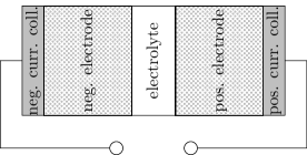
Following [27], we consider a pore-scale battery model based on [20]. The computational domain is divided into five parts: electrolyte, positive/negative electrode, positive/negative current collector (Fig. 1). On each of these subdomains, partial differential equations are given for the Li-ion concentration $c$ and the electrical potential $\phi$.

For the electrolyte we have

$$\frac{\partial c}{\partial t}-\nabla\cdot(D_{e}\nabla c) =0,$$ (1)

$$-\nabla\cdot\Bigl{(}\kappa\frac{1-t_{+}}{F}RT\frac{1}{c}\nabla c-\kappa\nabla\phi\Bigr{)} =0,$$ (2)

where $D_{e}=1.622\cdot 10^{-6}\frac{cm^{2}}{s}$, $\kappa=0.02\frac{s}{cm}$, $t_{+}=0.39989$ denote the collective interdiffusion coefficient in the electrolyte, the ion conductivity, and the transference number. $R=8.314\frac{J}{mol\,K}$, $F=96487\frac{As}{mol}$ are the universal gas constant and the Faraday constant. We fix the global temperature $T$ to $298K$.

In the electrodes, $c$ and $\phi$ satisfy

$$\frac{\partial c}{\partial t}-\nabla\cdot(D_{s}\nabla c) =0,$$ (3)

$$-\nabla\cdot(\sigma\nabla\phi) =0,$$ (4)

where $D_{s}=10^{-10}\frac{cm^{2}}{s}$ is the ion diffusion coefficient in the electrodes, and $\sigma=10\frac{s}{cm}$ ($\sigma=0.38\frac{s}{cm}$) in the negative (positive) electrode denotes the electronic conductivity.

Finally, no Li-ions can enter the current collectors, so $c=0$ on the whole current collector subdomains. Moreover, $\phi$ again satisfies

$$-\nabla\cdot(\sigma\nabla\phi)=0,$$ (5)

with $\sigma=10\frac{s}{cm}$ ($\sigma=0.38\frac{s}{cm}$) for the negative (positive) current collector.

Note that for this in comparison to [20] slightly simplified model (assuming constant $t_{+}$), the equations (1), (3) are linear and decoupled from the potential equations. However, the coupling between the two variables is established by the interface conditions at the electrode-electrolyte interfaces, where the so-called Butler-Volmer kinetics are assumed: the electric current (ion flux) $j$ (N) from the electrodes into the electrolyte is given by

$$j=2k\sqrt{c_{e}c_{s}(c_{max}-c_{s})}\sinh\left(\frac{\phi_{s}-\phi_{e}-U_{0}(\frac{c_{s}}{c_{max}})}{2RT}\cdot F\right),\quad N=\frac{j}{F}.$$ (6)

Here, $c_{e/s}$ ($\phi_{e/s}$) denotes the Li-ion concentration (electrical potential) at the electrolyte/electrode side of the interface. $c_{max}=24681\cdot 10^{-6}\frac{mol}{cm^{3}}$ ($c_{max}=23671\cdot 10^{-6}\frac{mol}{cm^{3}}$) denotes the maximum Li-ion concentration in the negative (positive) electrode, and the rate constant $k$ is given by $k=0.002\frac{Acm^{2.5}}{mol^{1.5}}$ at the negative and by $k=0.2\frac{Acm^{2.5}}{mol^{1.5}}$ at the positive electrode interface. Finally, the open circuit potential is given by $U_{0}(s)=(-0.132+1.41\cdot e^{-3.52s})V$ for the negative, and by

$$U_{0}(s)= \Bigl{[}\ 0.0677504\cdot\tanh(-21.8502\cdot s+12.8268)$$ (7)

$$\ -0.105734\cdot\bigl{(}(1.00167-s)^{-0.379571}-1.576\bigr{)}$$

$$\ -0.045\cdot e^{-71.69\cdot s^{8}}+0.01\cdot e^{-200\cdot(s-0.19)}+4.06279\ \Bigr{]}\cdot V$$

for the positive electrode.

Given the porous electrode structures, these interface conditions apply to a large surface area, giving this model highly nonlinear dynamics.

Finally, the system is closed by the following boundary conditions: homogeneous Neumann conditions for $c$ at all further inner and external domain boundaries, continuity conditions for $\phi$ at the current collector-electrode interfaces, homogenous Neumann conditions for $\phi$ at the current collector-electrolyte interfaces, $\phi\equiv U_{0}(c(0)/c_{max})$ at the negative current collector boundary, and $-n\cdot\sigma\nabla\phi\equiv\mu$ at the positive current collector boundary.

We consider the fixed charge rate $\mu$ as a parameter we want to vary in our numerical experiments.

2.2 Reduced basis method and empirical interpolation

After cell-centered finite volume discretization of the model on a voxel grid, replacing the numerical fluxes by the Butler-Volmer relations at the electrode-electrolyte interfaces, and backward Euler time discretization, we arrive at nonlinear, discrete equations systems of the form

$$\begin{bmatrix}\frac{1}{\Delta t}(c_{\mu}^{(t+1)}-c_{\mu}^{(t)})\\ 0\end{bmatrix}+A_{\mu}\left(\begin{bmatrix}c_{\mu}^{(t+1)}\\ \phi_{\mu}^{(t+1)}\end{bmatrix}\right)=0,\qquad(c_{\mu}^{(t)},\phi_{\mu}^{(t)})\in V_{h}\oplus V_{h},$$ (8)

where $A_{\mu}$ denotes the parametric finite volume space differential operator acting on the finite volume space $V_{h}$ (see [28] for a detailed derivation). Solving these systems using Newton’s method requires many hours for realistic geometries, even when using advanced algebraic multigrid solvers for computing the Newton updates.

Projection-based parametric model reduction methods are based on the idea of finding problem adapted approximation spaces $\tilde{V}\subseteq V_{h}\oplus V_{h}$ in which a reduced order solution is obtained by projection of the original equation system:

$$P_{\tilde{V}}\left\{\begin{bmatrix}\frac{1}{\Delta t}(\tilde{c}_{\mu}^{(t+1)}-\tilde{c}_{\mu}^{(t)})\\ 0\end{bmatrix}+A_{\mu}\left(\begin{bmatrix}\tilde{c}_{\mu}^{(t+1)}\\ \tilde{\phi}_{\mu}^{(t+1)}\end{bmatrix}\right)\right\}=0,\quad(\tilde{c}_{\mu}^{(t)},\tilde{\phi}_{\mu}^{(t)})\in\tilde{V}.$$ (9)

Here, $P_{\tilde{V}}$ denotes the orthogonal projection onto $\tilde{V}$. Since the manifold of system states $\{(c_{\mu}^{(t)},\phi_{\mu}^{(t)})\ |\ \mu\in[\mu_{min},\mu_{max}],\ t\in\{0,\ldots,T\}\}$ has a low-dimensional parametrization (by $(\mu,t)\in\mathbb{R}^{2})$, and assuming that this parametrization is sufficiently smooth, there is hope to find low-dimensional approximation spaces $\tilde{V}$ such that the model reduction error between the reduced solutions (9) and the corresponding high-dimensional solutions (8) is very small.

A vast amount of methods for constructing reduced spaces $\tilde{V}$ has been considered in literature. For time-dependent problems, the POD-Greedy method [14, 11] has shown to produce approximation spaces with quasi-optimal $l^{\infty}$-in-$\mu$, $l^{2}$-in-time reduction error. In our experiments below, we apply a more basic approach by computing a basis for $\tilde{V}$ via PODs of a pre-selected set of solution trajectories of (8). More precisely, we compute separate reduced concentration ($\tilde{V}_{c}$) and potential ($\tilde{V}_{\phi}$) spaces and let $\tilde{V}:=\tilde{V}_{c}\oplus\tilde{V}_{\phi}$. Due to the basic properties of POD, $\tilde{V}_{c}$, $\tilde{V}_{\phi}$ are $l^{2}$-in-$\mu$, $l^{2}$-in-time best-approximation spaces for the considered training set of solutions.

Even though the equation systems (9) are posed on the low-dimensional space $\tilde{V}$, solving (9) requires the evaluation of the projected operator $P_{\tilde{V}}\circ A_{\mu}$ (and its Jacobian), which in turn makes the computationally expensive evaluation of $A_{\mu}$ on the full finite volume space $V_{h}\oplus V_{h}$ necessary. The method of choice to overcome this limitation for nonlinear operators $A_{\mu}$ is empirical operator interpolation: $A_{\mu}$ is replaced by an interpolant $I_{M}\circ\tilde{A}_{M,\mu}\circ R_{M^{\prime}}$, where $\tilde{A}_{M,\mu}:\mathbb{R}^{M^{\prime}}\to\mathbb{R}^{M}$ is the restriction of $A_{\mu}$ to $M$ appropriately selected degrees of freedom (DOFs), $R_{M^{\prime}}:V_{h}\oplus V_{h}\to\mathbb{R}^{M\prime}$ is the restriction of the finite volume vectors to the $M^{\prime}$ DOFs required for the evaluation of $\tilde{A}_{M,\mu}$ and $I_{M}:\mathbb{R}^{M}\to V_{h}\oplus V_{h}$ is the linear combination with an appropriate interpolation basis (collateral basis). Due to the locality of finite volume operators, $M^{\prime}$ can be chosen such that $M^{\prime}\leq C\cdot M$, where $C$ only depends on the maximum number of neighboring cells in the given mesh. The interpolation DOFs and the associated collateral basis are obtained from solution snapshot data using the EI-Greedy algorithm [13, 9].

A direct application of this approach to $A_{\mu}$ would not be successful, however: since the collateral basis is contained in the linear span of operator evaluations on solution trajectories, the $\phi$-parts of the collateral basis vectors would, according to (8), completely vanish. Therefore, we first decompose $A_{\mu}$ as $A_{\mu}=A^{(const)}+\mu\cdot A^{(bnd)}+A^{(lin)}+A^{(1/c)}+A^{(bv)}$, where $A^{(1/c)}$, $A^{(bv)}$ are the nonlinear operators corresponding to $-\nabla\cdot\kappa\frac{1-t_{+}}{F}RT\frac{1}{c}\nabla c$ and the Butler-Volmer interfaces, $A^{(const)}$ ($A^{(bnd)}$) is the constant (parametric) part of $A_{\mu}$ corresponding to the boundary conditions, and $A^{(lin)}$ is the remaining linear part of $A_{\mu}$. We then apply empirical operator interpolation separately to $A^{(1/c)}$ and $A^{(bv)}$. With $T[\tilde{c}^{(t)}_{\mu}](\tilde{c},\tilde{\phi}):=(1/\Delta t\cdot(\tilde{c}-\tilde{c}_{\mu}^{(t)}),\ 0)$, we arrive at the fully reduced systems

$$\Bigl{\{}T[\tilde{c}^{(t)}_{\mu}] +P_{\tilde{V}}\circ A^{(const)}+\mu\cdot P_{\tilde{V}}\circ A^{(bnd)}+P_{\tilde{V}}\circ A^{(lin)}$$ (10)

$$+\{P_{\tilde{V}}\circ I_{M^{(1/c)}}^{(1/c)}\}\circ\tilde{A}_{M^{(1/c)},\mu}^{(1/c)}\circ R_{M^{\prime(1/c)}}^{(1/c)}$$

$$+\{P_{\tilde{V}}\circ I_{M^{(bv)}}^{(bv)}\}\circ\tilde{A}_{M^{(bv)},\mu}^{(bv)}\circ R_{M^{\prime(bv)}}^{(bv)}\ \ \ \Bigr{\}}\left(\begin{bmatrix}\tilde{c}_{\mu}^{(t+1)}\\ \tilde{\phi}_{\mu}^{(t+1)}\end{bmatrix}\right)=0.$$

After pre-computation of the linear maps $P_{\tilde{V}}\circ A^{(bnd)}$, $P_{\tilde{V}}\circ A^{(lin)}$, $P_{\tilde{V}}\circ I_{M^{(1/c)}}^{(1/c)}$, $R_{M^{\prime(1/c)}}^{(1/c)}$, $P_{\tilde{V}}\circ I_{M^{(bv)}}^{(bv)}$, $R_{M^{\prime(bv)}}^{(bv)}$ and of the constant map $P_{\tilde{V}}\circ A^{(const)}$ w.r.t. to a basis of $\tilde{V}$, (10) can be solved quickly and independent of the dimension of $V_{h}$.

2.3 Numerical experiments

Figure 2: Top left: small porous battery geometry used in numerical experiments. Size: $104\mu m\times 40\mu m\times 40\mu m$, $4.600$ DOFs, coloring indicates Li⁺ concentration at end of simulation, electrolyte not depicted. Top right: average solution time in seconds vs. dimension of reduced space $\tilde{V}$ and number of interpolation points ($M:=M^{(1/c)}+M^{(bv)}$). Bottom: relative model reduction errors (11) for concentration (left) and potential (right) variable vs. dimension of reduced space and number of interpolation points. A training set of 20 equidistant parameters was used for the generation of $\tilde{V}$ and the interpolation data, $\#\mathcal{S}_{test}=20$.

Figure 3: Porous battery geometry used in the numerical experiments. Size: $246\mu m\times 60\mu m\times 60\mu m$, $1.749.600$ DOFs, coloring indicates Li⁺ concentration at end of simulation, electrolyte not depicted.

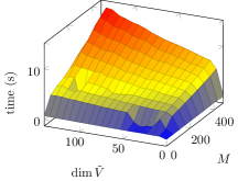
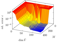
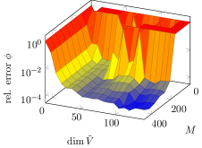
We consider two different test cases: a small test geometry (Fig. 2) which still exhibits the most important properties of a real battery geometry, and a large, fully resolved geometry (Fig. 3) useable for real-world simulations. In both cases, the initial Li⁺ concentration $c_{0}$ was set to $c_{0}\equiv 2639\cdot 10^{-6}\frac{mol}{cm^{3}}$ ($c_{0}\equiv 20574\cdot 10^{-6}\frac{mol}{cm^{3}}$) for the positive (negative) electrode and to $c_{0}\equiv 1200\cdot 10^{-6}\frac{mol}{cm^{3}}$ in the electrolyte. The model was simulated on a $T=2000s$ ($T=1600s$) time interval for the small (large) geometry, with a time step size of $\Delta t=20s$. The charge rate $\mu$ was for each simulation chosen as a constant from the interval $\bigl{[}0.00012\frac{A}{cm^{2}},0.0012\frac{A}{cm^{2}}\bigr{]}$ for the small and from the interval $\bigl{[}0.000318\frac{A}{cm^{2}},0.00318\frac{A}{cm^{2}}\bigr{]}$ for the large geometry.

To generate the reduced space $\tilde{V}$, we computed solution snapshots on training sets $\mathcal{S}_{train}$ of equidistant parameters. For the small geometry we chose $\#\mathcal{S}_{train}=20$, whereas for the large geometry we only selected the lower and upper boundary of the considered parameter domain, i.e. $\#\mathcal{S}_{train}=2$. For the generation of the empirical interpolation data using the EI-Greedy algorithm, we additionally included the evaluations of $A_{\mu}^{(1/c)}$ and $A_{\mu}^{(bv)}$ on all intermediate Newton stages of the selected solution trajectories.

As a measure for the model reduction error we consider the relative $l^{\infty}$-in-$\mu$, $l^{\infty}$-in-time error given by

$$\max_{\mu\in\mathcal{S}_{test}}\ \max_{t\in\{0,1,\ldots T/\Delta t\}}\ \frac{\|u_{\mu}^{(t)}-\tilde{u}_{\mu}^{(t)}\|}{\max_{t\in\{0,1,\ldots T/\Delta t\}}\|u_{\mu}^{(t)}\|},$$ (11)

where $u$ ($\tilde{u}$) is the concentration or potential part of the (reduced) solution and $\mathcal{S}_{test}$ denotes a random set of test parameters.

All simulations of the high-dimensional model have been performed with the battery simulation software BEST [21], which has been integrated with our model order reduction library pyMOR [27, 22]. The experiments were conducted as single-threaded processes on a dual socket compute server equipped with two Intel Xeon E5-2698 v3 CPUs with 16 cores running at 2.30 GHz each and 256GB of memory available.

For the small test geometry, we observe a rapid decay of the model reduction error for both the concentration and the potential variable (Fig. 2). As usual for empirical operator interpolation, we see that the number of interpolation points has to be increased for larger reduced space dimensions in order to ensure stability of the reduced model. Doing so, we obtain relative reduction errors as small as $10^{-4}$ with simulation times of less than $15s$.

Since we only selected 2 solution trajectories for the generation of the reduced model for the large geometry, we cannot expect such small model reduction errors over the whole parameter domain. In fact, the error stagnates already for relatively small reduced space dimensions (Table 2.3). Nevertheless, we easily achieve errors of less than one percent for a simulation time of $80s$. With an average solution time for the high-dimensional model of over 6 hours, we achieve at this error a speedup factor of 285.

Note that the solution time of the reduced model is still significantly larger than for the small geometry. This can be attributed to the fact that the localized evaluation of $A_{\mu}^{(1/c)}$, $A_{\mu}^{(bv)}$ has been only partially implemented in BEST and still requires operations on high-dimensional data structures. After the implementation of localized operator evaluation in BEST has been finalized, we expect even shorter simulation times.

Table 1: Relative model reduction errors (11) and reduced simulation times for the large battery geometry (Fig. 3). 188 interpolation points, average time for solution of the high-dimensional model: $22979s$, $\#\mathcal{S}_{test}=10$.

$\dim\tilde{V}$	11	21	30	40
rel. error $c$	$9.26\cdot 10^{-3}$	$3.96\cdot 10^{-3}$	$3.05\cdot 10^{-3}$	$2.93\cdot 10^{-3}$
rel. error $\phi$	$2.07\cdot 10^{-3}$	$1.50\cdot 10^{-3}$	$1.46\cdot 10^{-3}$	$1.26\cdot 10^{-3}$
time (s)	82	81	79	81
speedup	279	285	290	283

3 Localized reduced basis multiscale approximation of heat conduction

The microscale battery model in Section 2 is considered under the assumption of constant global temperature $T$. In general, it is desirable to couple this model with a spatially resolved model for the temperature distributions within the battery. For the model reduction of such heat conduction in porous electrodes we present a first application of the localized reduced basis multiscale Method (LRBMS) for parabolic PDEs.

In this first step we consider the simulation and model reduction of heat conduction separately from what is presented in Section 2 as a basis for a coupled simulation and model reduction in future work.

For an introduction of the LRBMS for elliptic parameterized multiscale problems and recent results concerning localized a posteriori error estimation and online enrichment, we refer to [26].

3.1 A battery - heat conduction model with resolved electrode geometry

We consider here the same spatially resolved 3D pore-scale battery geometry (cf. Fig. 3) as in Section 2, where the computational domain is composed of five materials which are of interest for thermal modeling, that is: electrolyte, positive/negative electrode and positive/negative current collectors, each with possibly different thermal conductivities.

As a simplified model for heat conductivity within a battery with spatially resolved electrodes, we consider a parabolic PDE for the temperature $T$ of the form

$$\frac{\partial T}{\partial t}-\nabla\cdot\big{(}D\,\nabla T\big{)}=Q,$$ (12)

together with suitable initial and boundary conditions. Here $D$ denotes the space-dependent conductivity tensor, which is material specific and thus takes different values in the current collectors, the porous electrodes, the separator, and the electrolyte. Hence, $D$ inherits the highly heterogeneous structure of the porous electrodes and thus has an intrinsic multiscale character. In general, $Q$ collects all heat generating sources, such as heat generation due to electrochemical reaction, reversible heat and ohmic heat, each of which may in turn depend on the Li-ion concentration and the electric potential and thus vary in space and time. These sources arise in particular due to the electrochemical reaction at the interface between the electrodes and the electrolyte and it is thus desirable to consider the full 3D pore-scale battery model in order to get an insight into possible variations of the temperature within the battery. We refer, e.g. to [6, 5] for a more detailed derivation of an energy balance equation for Lithium-Ion batteries and corresponding simulation schemes.

Depending on the study in question, any of the sources, the thermal conductivity or the initial or boundary values may depend on a low-dimensional parameter vector $\mu$.

3.2 Localization of reduced basis methods - LRBMS

As a first step towards a realistic model we allow for parametric thermal conductivities and presume stationary sources and boundary values. Thus, a (spatial) discretization of (12) by a suitable discretization scheme (such as finite volumes or continuous or discontinuous Galerkin (DG) finite elements) and a backward Euler time-discretization yield a set of linear equations of the form,

$$\tfrac{1}{\Delta t}M_{h}\big{(}T^{(t+1)}-T^{(t)}\big{)}+B_{h,\mu}\,T^{(t+1)}=Q_{h}, T^{(t+1)}\in V_{h},$$ (13)

to be solved in each time step, where $M_{h}$ and $B_{h,\mu}$ denote the discrete $L^{2}$-inner product and parametric space differential operators induced by the spatial discretization, respectively, which act on the corresponding high-dimensional discrete space $V_{h}$. In addition, $Q_{h}$ denotes the discrete representation of the source and boundary values.

To obtain a reduced order model for the discrete heat conduction model (13), we proceed in an analog way, as described in Section 2 above, by a Galerkin projection onto a problem adapted reduced approximation space $\tilde{V}\subset V_{h}$. Once $\tilde{V}$ is given, we obtain the set of reduced equations for each time step:

$$\tfrac{1}{\Delta t}\tilde{M}\big{(}\tilde{T}^{(t+1)}-\tilde{T}^{(t)}\big{)}+\tilde{B}_{\mu}\,\tilde{T}^{(t+1)}=\tilde{Q}, \tilde{T}^{(t+1)}\in\tilde{V},$$ (14)

where $\tilde{M}$, $\tilde{B}_{\mu}$ and $\tilde{Q}$ denote the reduced operators and functionals, respectively, acting on the low-dimensional reduced space $\tilde{V}$. Since all operators and functionals arising in (14) are affinely decomposable with respect to the low-dimensional parameter vector $\mu$ (given for instance the thermal conductivity as in Section 3.3) and linear with respect to $\tilde{V}$, we can precompute their respective evaluations in a computationally expensive offline step, e.g., by $\tilde{M}=\underline{P_{\tilde{V}}}^{\bot}\underline{M_{h}}\;\underline{P_{\tilde{V}}}$, where $\underline{M_{h}}$ and $\underline{P_{\tilde{V}}}$, respectively, denote the matrix representations of $M_{h}$ and of the orthogonal projection $P_{\tilde{V}}:V_{h}\to\tilde{V}$ with respect to the basis of $V_{h}$. Online, for each new input parameter $\mu$, we can then quickly solve the reduced low-dimensional problem (14) to obtain a low-dimensional representation of the temperature $\tilde{T}$, which can be post-processed to obtain the original temperature $T$, if required, or a derived quantity of interest.

As mentioned above, the problem adapted reduced space $\tilde{V}$ can be adaptively generated by an iterative POD-Greedy procedure [14]: in each step of the greedy algorithm, given an error estimate on the model reduction error, a full high-dimensional solution trajectory for the hitherto worst-approximated parameter is computed and the most dominant POD modes of the projection error of this trajectory are added to the reduced basis spanning $\tilde{V}$.

This procedure has been shown to produce quasi-optimal low-dimensional reduced order models which successfully capture the dynamics of the original high-dimensional model [11]. However, in the context of multiscale phenomena or highly resolved geometries, such as the porous structures within a Li-ion battery, the computational cost required to generate the reduced model can become unbearably large, even given modern computing hardware.

As a remedy, the localized reduced basis multiscale method has been introduced for stationary elliptic multiscale problems [18, 1] to lower the computational burden of traditional RB methods by generating several local reduced bases associated with a partitioning of the computational domain. The local quantities associated with these individual subdomains can be projected independently in parallel. In [25, 26], the LRBMS was extended to additionally account for the discretization error and to allow for an adaptive enrichment of the local reduced approximation spaces, which may even eliminate the need for global solution snapshots at all.

In this contribution, we demonstrate a first application of the LRBMS to parabolic multiscale problems, such as spatially resolved heat conduction in a Lithium-Ion battery. We therefore discretize (12) locally by a standard finite element or discontinuous Galerkin scheme independently in each subdomain of a given partitioning of the computational domain and couple the arising local operators, products and functionals along these subdomains by symmetric weighted interior penalty discontinuous Galerkin fluxes (cf. [26] and the references therein). We use the resulting discretization to compute global solution snapshots during the greedy algorithm, as detailed above. However, instead of a single reduced basis with global support, we iteratively generate local reduced bases on each subdomain by localizing the solution trajectories with respect to each subdomain and by carrying out local PODs for further localized compression in a post-processing step.

The resulting reduced space is then given as the direct sum of the local reduced approximation spaces spanned by these local reduced bases. Accordingly, we obtain the reduced problem (14) by local Galerkin projections of the local operators and functionals and coupling operators associated with each subdomain and its neighbor, yielding sparse reduced quantities.

3.3 Numerical experiments

Figure 4: Error evolution during the POD-Greedy basis generation to reach a target absolute error of $10^{-10}$ for the numerical experiment from Section 3.3. Depicted is the $L^{\infty}$-in-$\mu$, $L^{\infty}$-in-$t$, and $H^{1}$-in-space error over the set of five equidistant training samples in $[0.1;10]$.

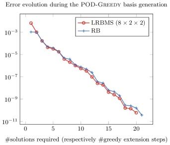
To demonstrate the applicability of the LRBMS we conduct an experiment on the same geometry used in the larger experiment in Section 2.3 (compare Figure 3). For the thermal conductivities we choose constant values within each material (the positive/negative electrode and the positive/negative current collectors), as reported in [6, 4th column of Table 4]. Within the electrolyte we allow to vary the constant thermal conductivity within the range $\mu\in[0.1;10]$. We pose homogeneous Dirichlet boundary values at the current collectors and homogeneous Neumann boundary values elsewhere and start the simulations with an initial temperature of 0K, using ten time steps to reach the final time $10^{-3}$. For the heat source we set $Q=10^{3}$ within the electrodes and $Q=0$ within the current collectors and the electrolyte. While this is not necessarily a physically meaningful setup, it inherits the computational challenges of a realistic model, namely a highly resolved geometry, discontinuous thermal conductivities depending on the materials and heat sources which align with the geometry of the different materials.

We triangulate the computational domain with $5,313,600$ simplexes and compare the LRBMS using $8\times 2\times 2$ subdomains to a standard RB method (which corresponds to choosing one subdomain). Within each subdomain, we use the same SWIPDG discretization as for the coupling, thus yielding comparable discretizations with $21,254,400$ degrees of freedom in both approaches. As an estimate on the model reduction error we use the true $L^{\infty}$-in-time, $H^{1}$-in-space error.

The discretization is implemented within the DUNE numerics environment [4, 3], centered around dune-gdt [23]: the dune-stuff [24] module provides classes for vectors, matrices and linear solvers (for instance the bicgstab.amg.ilu0 solver used in these experiments), dune-gdt provides the discretization building blocks (such as discrete function spaces, operators, products and functionals), and dune-hdd provides parametric discretizations compatible with pyMOR [22]. Finally, dune-pymor is used, as it provides the Python-bindings and wrappers to integrate the DUNE-code with our model reduction framework pyMOR. The experiments were conducted on the same compute server as described in Section 2.3.

As we observe from Fig. 4, both the LRBMS and the standard RB method show comparable exponential error decay. In general, the quality of the reduced spaces generated by the LRBMS is slightly better, while requiring less detailed solution snapshots to reach the same target error.

Table 2: Comparison of runtimes of the experiments from Section 3.3. Setup time includes grid generation, subdomain partitioning and assembly of operators, products and functionals. POD-Greedy time includes error estimation, generation of the reduced basis and the reduced basis projection. The average time to solve the detailed problem is $2h28m5s$.

	setup	POD-Greedy	reduced basis size	solution time
RB	$26m47s$	$14h41m52s$	21	$35s$
LRBMS	$36m7s$	$14h34m39s$	$32\times 20$	$35s$

As can be seen from Table 2, the POD-Greedy basis generation using 32 subdomains is slightly faster than the basis generation using a single subdomain. However, since the experiments were conducted as single-threaded processes and since the LRBMS allows for parallel local PODs and parallel local reduced basis projections, the basis generation time of the LRBMS can be further accelerated significantly.

4 Conclusion

In this contribution we have demonstrated the efficient applicability of recent model reduction approaches, such as the POD-Greedy reduced basis method, the empirical operator interpolation, and the localized reduced basis multiscale method (LRBMS) for efficient simulation of real world problems, such as 3D spatially resolved heterogeneous Lithium-Ion battery models. The demonstrated model reduction approaches are realized within our model order reduction library pyMOR [27, 22] with bindings, both to the battery simulation software BEST [21], and the general purpose Distributed and Unified Numerics Environment DUNE [4, 3], employing the dune-gdt, dune-stuff, and dune-hdd discretization and solver backends. Speedup factors of about 285 were obtained for the full strongly non-linear battery model in Section 2 using the reduced basis method with empirical operator interpolation [9], and around 253 for the linear parabolic heat conduction model in Section 3 using a parabolic extension of the localized reduced basis multiscale method [26].

Acknowledgement

The authors thank Sebastian Schmidt from Fraunhofer ITWM Kaiserslautern for the close and fruitful collaboration within the BMBF-project MULTIBAT towards integration of BEST with pyMOR.

References

- [1] F. Albrecht, B. Haasdonk, S. Kaulmann, and M. Ohlberger, The localized reduced basis multiscale method, ALGORITMY 2012 - Proceedings of contributed papers and posters (A. Handlovicova, Z. Minarechova, and D. Cevcovic, eds.), vol. 1, Slovak University of Technology in Bratislava, Publishing House of STU, April 2012, pp. 393–403.
- [2] M. Barrault, Y. Maday, N. Nguyen, and A. Patera, An “empirical interpolation” method: application to efficient reduced-basis discretization of partial differential equations, Comptes Rendus de l’Académie des Sciences, Series I 339 (2004), 667–672.
- [3] P. Bastian, M. Blatt, A. Dedner, C. Engwer, R. Klöfkorn, R. Kornhuber, M. Ohlberger, and O. Sander, A generic grid interface for parallel and adaptive scientific computing. II. Implementation and tests in DUNE, Computing 82:2-3 (2008), 121–138.
- [4] P. Bastian, M. Blatt, A. Dedner, C. Engwer, R. Klöfkorn, M. Ohlberger, and O. Sander, A generic grid interface for parallel and adaptive scientific computing. I. Abstract framework, Computing 82:2-3 (2008), 103–119.
- [5] L. Cai and R. White, Reduction of model order based on proper orthogonal decomposition for lithium-ion battery simulations, Journal of the Electrochemical Society 156:3 (2009), A154–A161, cited By 67.
- [6] S. C. Chen, C. C. Wan, and Y. Y. Wang, Thermal analysis of lithium-ion batteries, Journal of Power Sources 140 (2005), 111 – 124.
- [7] F. Ciucci and W. Lai, Derivation of micro/macro lithium battery models from homogenization, Transp. Porous Media 88:2 (2011), 249–270.
- [8] M. Doyle, T. Fuller, and J. Newman, Modeling of galvanostatic charge and discharge of the lithium/ polymer/insertion cell, Journal of the Electrochemical Society 140:6 (1993), 1526–1533, cited By 789.
- [9] M. Drohmann, B. Haasdonk, and M. Ohlberger, Reduced basis approximation for nonlinear parametrized evolution equations based on empirical operator interpolation, SIAM Journal on Scientific Computing 34:2 (2012), A937–A969.
- [10] S. Golmon, K. Maute, and M. L. Dunn, Multiscale design optimization of lithium ion batteries using adjoint sensitivity analysis, Internat. J. Numer. Methods Engrg. 92:5 (2012), 475–494.
- [11] B. Haasdonk, Convergence rates of the POD-Greedy method, M2AN Math. Model. Numer. Anal. 47 (2013), 859–873.
- [12] B. Haasdonk, Reduced basis methods for parametrized PDEs – A tutorial introduction for stationary and instationary problems, Tech. report, 2014, Chapter to appear in P. Benner, A. Cohen, M. Ohlberger and K. Willcox: ”Model Reduction and Approximation: Theory and Algorithms”, SIAM.
- [13] B. Haasdonk, M. Ohlberger, and G. Rozza, A reduced basis method for evolution schemes with parameter-dependent explicit operators, Electron. Trans. Numer. Anal. 32 (2008), 145–161.
- [14] B. Haasdonk and M. Ohlberger, Reduced basis method for finite volume approximations of parametrized linear evolution equations, M2AN Math. Model. Numer. Anal. 42:2 (2008), 277–302.
- [15] J. S. Hesthaven, G. Rozza, and B. Stamm, , SpringerBriefs in Mathematics, Springer International Publishing, 2016.
- [16] O. Iliev, A. Latz, J. Zausch, and S. Zhang, On some model reduction approaches for simulations of processes in Li-ion battery., Proceedings of Algoritmy 2012, conference on scientific computing, Vysoké Tatry, Podbanské, Slovakia, Slovak University of Technology in Bratislava, 2012, pp. 161–171.
- [17] S. Kaulmann, B. Flemisch, B. Haasdonk, K.-A. Lie, and M. Ohlberger, The Localized Reduced Basis Multiscale method for two-phase flows in porous media, Internat. J. Numer. Methods Engrg. 102:5 (2015), 1018–1040.
- [18] S. Kaulmann, M. Ohlberger, and B. Haasdonk, A new local reduced basis discontinuous Galerkin approach for heterogeneous multiscale problems, C. R. Math. Acad. Sci. Paris 349:23-24 (2011), 1233–1238.
- [19] O. Lass and S. Volkwein, Parameter identification for nonlinear elliptic-parabolic systems with application in lithium-ion battery modeling, Comput. Optim. Appl. 62:1 (2015), 217–239.
- [20] A. Latz and J. Zausch, Thermodynamic consistent transport theory of li-ion batteries, Journal of Power Sources 196:6 (2011), 3296 – 3302.
- [21] G. B. Less, J. H. Seo, S. Han, a. M. Sastry, J. Zausch, a. Latz, S. Schmidt, C. Wieser, D. Kehrwald, and S. Fell, Micro-Scale Modeling of Li-Ion Batteries: Parameterization and Validation, Journal of The Electrochemical Society 159:6 (2012), A697.
- [22] R. Milk, S. Rave, and F. Schindler, pyMOR - generic algorithms and interfaces for model order reduction, arXiv e-prints 1506.07094 (2015), http://arxiv.org/abs/1506.07094.
- [23] R. Milk and F. Schindler, dune-gdt (http://dx.doi.org/10.5281/zenodo.35389), 2015.
- [24] , dune-stuff (http://dx.doi.org/10.5281/zenodo.35390), 2015.
- [25] M. Ohlberger and F. Schindler, A-posteriori error estimates for the localized reduced basis multi-scale method, Finite Volumes for Complex Applications VII-Methods and Theoretical Aspects (J. Fuhrmann, M. Ohlberger, and C. Rohde, eds.), Springer Proceedings in Mathematics & Statistics, vol. 77, Springer International Publishing, may 2014, pp. 421–429.
- [26] , Error control for the localized reduced basis multi-scale method with adaptive on-line enrichment, SIAM J. Sci. Comput. 37:6 (2015), A2865–A2895.
- [27] M. Ohlberger, S. Rave, S. Schmidt, and S. Zhang, A model reduction framework for efficient simulation of li-ion batteries, Finite volumes for complex applications. VII. Elliptic, parabolic and hyperbolic problems, Springer Proc. Math. Stat., vol. 78, Springer, Cham, 2014, pp. 695–702.
- [28] P. Popov, Y. Vutov, S. Margenov, and O. Iliev, Finite volume discretization of equations describing nonlinear diffusion in li-ion batteries, Numerical Methods and Applications (I. Dimov, S. Dimova, and N. Kolkovska, eds.), Lecture Notes in Computer Science, vol. 6046, Springer Berlin Heidelberg, 2011, pp. 338–346.
- [29] A. Quarteroni, A. Manzoni, and F. Negri, , La Matematica per il 3+2, Springer International Publishing, 2016.
- [30] V. Taralova, Upscaling approaches for nonlinear processes in lithium-ion batteries, Ph.D. thesis, 2015, pp. VII, 224.
- [31] A. Wesche and S. Volkwein, The reduced basis method applied to transport equations of a lithium-ion battery, COMPEL: The International Journal for Computation and Mathematics in Electrical and Electronic Engineering 32 (2013), 1760–1772.