Exact symmetries in the velocity fluctuations of a hot Brownian swimmer

Abstract

Symmetries constrain dynamics. We test this fundamental physical principle, experimentally and by molecular dynamics simulations, for a hot Janus swimmer operating far from thermal equilibrium. Our results establish scalar and vectorial steady-state fluctuation theorems and a thermodynamic uncertainty relation that link the fluctuating particle current to its entropy production at an effective temperature. A Markovian minimal model elucidates the underlying non-equilbrium physics.

Throughout the 19th century, Brownian motion was studied intensively but remained a confusing and enigmatic phenomenon. Even excessive experimental data for the velocity of colloidal particles did not seem to allow for a conclusive characterization of the motion, until interpreted as mean-square spatial displacements within a consistent theory of Brownian fluctuations Einstein (1905). The main point is that the mean-square displacement is robust with respect to the chosen time discretization of the trajectory, while the velocity is not. Nevertheless, the infamous velocity of Brownian particles has recently gained renewed conceptual and practical interest. This is partly due to improved technical abilities to assess its regular short-time limit Franosch et al. (2011); Kheifets et al. (2014), and partly to a surge of applications involving self-propelled colloidal particles Marchetti et al. (2013). The directed autonomous motion of such “Brownian swimmers” can be harnessed for performing mechanical work and other potentially useful tasks Ebbens and Howse (2010), but its persistence is limited by Brownian fluctuations. In the following, we demonstrate that these fluctuations are not completely chaotic but encode a characteristic fingerprint of the underlying space-time symmetry, even far from thermal equilibrium.

We specifically consider a so-called hot Brownian swimmer, in theory, experiment, and computer simulations. The swimmer is designed as a Janus sphere made of two hemispheres with unequal thermal and solvation properties, which excites phoretic surface flows upon heating. A variety of such phoretic self-propulsion mechanisms is commonly employed in the design of artificial microswimmers. They all rely on the creation of asymmetric gradients of a thermodynamic field (e.g. concentration of a solute Howse et al. (2007), temperature Jiang et al. (2010)) in the solvent, which induces a systematic drift through classical interfacial phoretic processes Anderson (1989). Besides their biomimetic and practical relevance for promising applications in nano-science, self-propelled particles are of fundamental interest as paradigmatic non-equilibrium systems. Their energy input is not due to fluxes at the boundary, as often the case in macroscopically induced non-equilibrium states, but localized on the particle scale. And their self-propulsion is not due to a balance of external body forces with Stokes friction, as assumed in popular “dry-swimmer” models Marchetti et al. (2013). Instead, they are characterized by (hydrodynamic) long-range interactions very different from those found in driven colloids. In other words, microswimmers are not simply ordinary driven colloids in disguise. As a result, their collective behavior displays peculiar features, such as phases and phase transitions absent in sheared and sedimenting colloids, say Golestanian (2012); Theurkauff et al. (2012). But clear non-equilibrium signatures are detected already on the single-particle level. Examples include non-Gaussian fluctuations Zheng et al. (2013), negative mobility for confined swimmers Ghosh et al. (2014), and hot Brownian motion Rings et al. (2010) for non-isothermal swimmers. Despite the possibility to experimentally track and manipulate single particle trajectories Bregulla et al. (2014), a less explored direction of research is the study of fluctuations of (thermodynamic) path observables, defined along trajectories, as in stochastic energetics Sekimoto (2010); Seifert (2012). In particular, one may wonder whether fluctuation theorems are valid for self-propelled particles.

Fluctuation theorems are symmetry relations holding for a wide class of non-equilibrium systems Evans et al. (1993); Gallavotti and Cohen (1995); Kurchan (1998); Lebowitz and Spohn (1999); Maes (1999); Seifert (2005). They quantify the irreversibility of non-equilibrium processes by their total entropy production $S$, saying that the probability $P(S)$ for positive $S$ is exponentially larger than for negative $S$:

$$P(S)=P(-S)e^{S/k_{B}}.$$ (1)

Such relations ultimately originate from the time-reversal invariance of the microscopic dynamics that is broken at the ensemble level by a non-conservative driving. More recently, additional fluctuation theorems were identified, which rely on the breaking of spatial symmetries of the underlying microscopic dynamics Hurtado et al. (2011, 2014); Kumar et al. (2015). They relate the probabilities of vectorial observables pointing in different directions, such as the isometric currents $\boldsymbol{J}$ and $\boldsymbol{J}^{\prime}$ (currents of equal strength in different directions) excited by a homogeneous driving force $\boldsymbol{\epsilon}$ in an isotropic system:

$$P(\boldsymbol{J})=P(\boldsymbol{J}^{\prime})e^{\boldsymbol{\epsilon}\cdot(\boldsymbol{J}-\boldsymbol{J}^{\prime})}\,.$$ (2)

For our hot Brownian swimmers (and other self-propelled particles), the validity of Eqs. (1) and (2) is a priori in doubt. First, the phoretic mechanism responsible for the entropy production is not an external deterministic driving, as usually assumed to derive Eqs. (1) and (2). In addition, due to the presence of strong and long-ranged thermodynamic gradients, the solvent is not an equilibrium bath. Hence, the thermal noise need not be Gaussian as invoked in proofs of fluctuation relations for noisy dynamics. In case of a particle generating a temperature gradient, the bath noise does not even possess a definite temperature but is generally characterized by a nontrivial noise temperature spectrum arising from hydrodynamic memory Joly et al. (2011); Falasco et al. (2014a). Finally, Eq. (2) has been proved so far only for models that do not include inertia Pérez-Espigares et al. (2015). Despite all that, we now verify the fluctuation relations (1) and (2) relating the entropy production and the particle current for a hot Brownian swimmer both experimentally and numerically. A minimal analytical model helps to rationalize our findings.

The experimental system consists of a polystyrene bead of $500~{}\text{nm}$ radius, half-coated with a $50~{}\text{nm}$ thick gold layer, in aqueous solution. It is narrowly confined between two glass plates coated with a non-ionic surfactant (Pluronic) to prevent the particle from sticking. The sample is illuminated through a dark field condenser, and the scattered light is collected and imaged with a CCD-camera. The particle’s center of mass position $\boldsymbol{r}$ and orientation $\boldsymbol{n}$ (a unit vector along the symmetry axis from hot to cold) are recorded at an inverse frame rate of $5~{}\text{ms}$. A $532~{}\text{nm}$ laser with incident intensity of $0.05~{}\text{mW}/\mu\text{m}^{2}$ continuously heats the particle. The piezo-position employed for the spatial positioning of the sample is adjusted every $100$ frames to keep the particle in the center of the Gaussian beam. The tangential surface gradient of the local temperature translates into a thermophoretic propulsion velocity $v_{\text{p}}\boldsymbol{n}$, stemming from the unbalanced particle-fluid interactions Anderson (1989) plus thermoosmotic contributions from the nearby glass covers Bregulla et al. (2016).

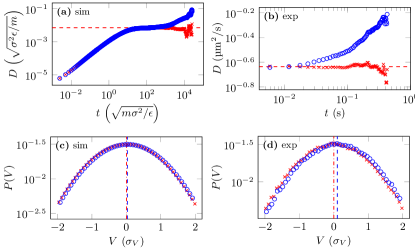
Figure 1: Upper panel: longitudinal ($\circ$) and transverse ($\times$) time-dependent diffusivities $D_{\|}$ and $D_{\perp}$ in the particle frame, as measured in simulation (a) and experiment (b). Their common plateau gives the diffusion constant $D$, and the late-time slope of $D_{\|}(t)$ the propulsion speed $v_{\text{p}}$. Lower panel: histograms of the corresponding short-time displacements.

A similar, but technically somewhat different realization of a hot swimmer was implemented numerically. We performed molecular dynamics simulations of $6\cdot 10^{4}$ Lennard–Jones (LJ) atoms of mass $m$. The $255$ atoms belonging to the spherical swimmer were additionally bonded by a FENE-potential Chakraborty et al. (2011). The standard LJ potential $4\epsilon\bigl{[}(\sigma/r)^{12}-c_{if}(\sigma/r)^{6}\bigr{]}$ was modified by introducing an effective wetting parameter $c_{if}$ for the interactions between the fluid ($f$) and the atoms composing the two hemispheres ($i=a,\,b$) of the particle surface. They serve to mimic the asymmetric solvent heating by the gold cap and polystyrene body of the experimental particle, in an efficient way Schachoff et al. (2015). We used $c_{af}=2$ and $c_{bf}=1$ for all simulations reported in this paper. In a typical simulation run, we first equilibrate the system in the Nosé-Hoover NVT ensemble at the prescribed temperature $T=0.75\epsilon/k_{B}$ and with an average number density $\sim 0.8\sigma^{-3}$ of fluid particles. Subsequently, we switch off the global thermostat and only the atoms near the boundary of the simulation box are kept at the ambient temperature, whereas the atoms on one half of the particle surface are heated to a substantially elevated temperature $T_{p}=1.5\epsilon/k_{B}$, by means of a standard velocity rescaling algorithm. After allowing the system to reach a steady state, we record time traces of the position $\boldsymbol{r}$ and velocity $\boldsymbol{V}$ of the particle’s center of mass, as well as the particle orientation $\boldsymbol{n}$. Differently from the experiment, the system is spatially isotropic in three dimensions.

We start our analysis with the time-dependent diffusion coefficients parallel and perpendicular to $\boldsymbol{n}$,

$$D_{\parallel}(t)=\frac{1}{2}\frac{\text{d}}{\text{d}t}{\left<\left(\int_{0}^{t}\text{d}\tau\boldsymbol{V}(\tau)\cdot\boldsymbol{n}(\tau)\right)^{2}\right>},$$ (3)

$$D_{\perp}(t)=\frac{1}{4}\frac{\text{d}}{\text{d}t}{\left<\left(\int_{0}^{t}\text{d}\tau\boldsymbol{V}(\tau)\cdot(\boldsymbol{1}-\boldsymbol{n}\boldsymbol{n}(\tau))\right)^{2}\right>},$$ (4)

where ${\left<\dots\right>}$ denotes steady-state ensemble averaging. As seen from Fig. 1a, the particle performs free diffusion in the perpendicular direction on times beyond the timescale $\tau_{\text{St}}$ ($\approx 10\sqrt{m\sigma^{2}/\epsilon}$ in the simulations) for velocity damping, given by the particle mass over the Stokes friction. This manifests itself as a plateau in $D_{\perp}(t)$, which can be used to read off the long-time translational diffusion constant as $D\equiv D_{\perp}(t\gg\tau_{\text{St}})$. Along the particle axis, the active drift $v_{\text{p}}={\left<\boldsymbol{n}\cdot\boldsymbol{V}\right>}$ (technically extracted from recorded trajectories by averaging over realizations and time) is superimposed as a ballistic component, so that $D_{\parallel}(t\gg\tau_{\text{St}})\sim D+v_{\text{p}}^{2}t$. Nevertheless, the mixing of parallel and perpendicular dynamics in the lab frame randomizes the particle orientation $\boldsymbol{n}(t)$ at late times, giving rise to an enhanced apparent overall diffusion coefficient. Note that all mentioned diffusion and mobility coefficients are non-equilibrium transport coefficients, since (global) thermal equilibrium is broken.

The data in Figs. 1c,d show that, despite the substantial thermal gradients attained in the simulations, the particle velocities parallel and perpendicular to $\boldsymbol{n}$ are essentially Gaussian distributed. This demonstrates that the thermal agitation of the Janus particle can be attributed to a Gaussian noise. It also implies that, at least for the swimmer, the fluid can effectively be described as locally in thermal equilibrium, which is indeed a necessary assumption in standard theories of phoretic transport and non-isothermal Langevin descriptions.

From the above observations, the following picture for the physics underlying Eqs. (1) and (2) emerges. On average, the particle will be propelled along the axis $\boldsymbol{n}$, or more generally, such that $\boldsymbol{n}\cdot\dot{\boldsymbol{r}}>0$. But on rare occasions, a fluctuation can displace the particle against the phoretic drift, such that $\boldsymbol{n}\cdot\dot{\boldsymbol{r}}<0$. The two dissimilar situations correspond to energy dissipation to the fluid and energy extraction from it, respectively. While the first conforms with the expected thermodynamic behavior, the second represents an atypical transient fluctuation. Their relative rate is exactly quantified by Eq. (1).

To formalize this intuitive picture, we now propose a minimal model for the swimmer dynamics. By restricting our analysis to times $t\gg\tau_{\text{St}}$, the Brownian fluctuations are effectively diffusive, and the particle momentum and all hydrodynamic modes can be taken as fully relaxed. Long-time tails and any randomness in the swimming speed $v_{\text{p}}$, which may arise from the fluctuating fluid momentum and temperature, are discarded. On this level, the stochastic motion of the hot Janus particle can be represented by the caricature of two isotropic Markov processes for its position and orientation vectors $\boldsymbol{r}(t)$ and $\boldsymbol{n}(t)$, with a superimposed constant drift along $\boldsymbol{n}(t)$. The corresponding overdamped Langevin equations read

$$\dot{\boldsymbol{r}}=v_{\text{p}}\boldsymbol{n}+\sqrt{2D}\boldsymbol{\xi}_{\rm t}\,,$$ (5)

$$\dot{\boldsymbol{n}}=\sqrt{2D_{\rm r}}\boldsymbol{\xi}_{\rm r}\times\boldsymbol{n}\,,$$ (6)

where $\boldsymbol{\xi}_{\rm t}(t)$ and $\boldsymbol{\xi}_{\rm r}(t)$ represent independent unbiased Gaussian white noise processes with unit variance.

We next consider the probability

$$P[{{\mathcal{X}}}]\propto\exp{\left(-\frac{1}{4D}\int_{0}^{t}\text{d}\tau\,[\dot{\boldsymbol{r}}(\tau)-v_{\text{p}}\boldsymbol{n}(\tau)]^{2}\right)}.$$ (7)

associated with a path ${{\mathcal{X}}}\equiv\{\{\boldsymbol{r}(\tau),\boldsymbol{n}(\tau)\}:0\leqslant\tau\leqslant t\}$ (the ordered set of positions and orientations in the time interval $[0,t]$). The path weight given by Eq. (6) is omitted, because it is inessential, as is the initial configuration $\{\boldsymbol{r}(0),\boldsymbol{n}(0)\}$, because all allowed configurations are equiprobable for an unconfined particle in the steady state. The probability $P[\tilde{{\mathcal{X}}}]$ to observe the same event backwards in time is obtained from Eq. (7) by the time reversal transformation $\tau\to t-\tau$. The two path weights are thus related by

$$P[{{\mathcal{X}}}]=P[\tilde{{\mathcal{X}}}]\exp{\left(\frac{v_{\text{p}}}{D}\int_{0}^{t}\text{d}\tau\;\dot{\boldsymbol{r}}(\tau)\cdot\boldsymbol{n}(\tau)\right)}\,,$$ (8)

saying that a path ${{\mathcal{X}}}$ resulting in a positive total displacement along $\boldsymbol{n}$ is exponentially more probable than the reversed path $\tilde{{\mathcal{X}}}$ resulting in a negative displacement. To show that this leads to a measurable asymmetry, we define a time-averaged forward velocity

$$j_{\|}[{{\mathcal{X}}}] \equiv\frac{1}{t}\int_{0}^{t}\text{d}\tau\;\dot{\boldsymbol{r}}(\tau)\cdot\boldsymbol{n}(\tau).$$ (9)

The probability that $j_{\|}[{\mathcal{X}}]$ attains a certain value, say $J_{\|}$, follows by multiplying both sides of Eq. (8) by $\delta(j_{\|}-J_{\|})$ and summing over all possible trajectories:

$$\sum_{{{\mathcal{X}}}}P[{{\mathcal{X}}}] \delta(j_{\|}-J_{\|})=\sum_{{{\mathcal{X}}}}P[\tilde{{\mathcal{X}}}]e^{\frac{v_{\text{p}}}{D}tj_{\|}}\delta(j_{\|}-J_{\|}).$$ (10)

The left-hand side of Eq. (10) is, by definition, $P(J_{\|})\equiv\textrm{Prob}(j_{\|}[{\mathcal{X}}]=J_{\|})$, while the right-hand side becomes

$$\sum_{\tilde{{\mathcal{X}}}}P[\tilde{{\mathcal{X}}}]e^{-\frac{v_{\text{p}}}{D}tj_{\|}}\delta(j_{\|}+J_{\|}) =P(-J_{\|})e^{\frac{v_{\text{p}}}{D}tJ_{\|}}$$

when we rewrite the sum over paths as sum over time-reversed paths and flip the sign of $j_{\|}$ accordingly, since $j_{\|}[{{\mathcal{X}}}]=-j_{\|}[\tilde{{\mathcal{X}}}]$. We thus obtain the fluctuation relation

$$\frac{1}{t}\ln\frac{P(J_{\|})}{P(-J_{\|})}=\frac{v_{\text{p}}}{D}J_{\|}.$$ (11)

It is valid for all observation times consistent with the Markov condition $t\gg\tau_{\text{St}}$. Differently from usual steady-state fluctuation relations, boundary terms corresponding to the density of states evaluated at times $0$ and $t$ are absent, being trivial constants. This enables us to verify the theory at relatively short times, which permits an efficient sampling of the negative tail of $P(J_{\|})$. Corresponding histograms constructed from the numerical and experimental data are shown in Fig. 2a, b. The logarithmic ratios of statistically relevant opposite bins conform nicely with Eq. (11), as shown in Fig. 2c.

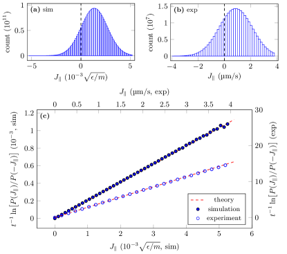
Figure 2: Upper panel: histograms of the longitudinal particle current $J_{\|}$, Eq. (9), as measured in simulation (a) and experiment (b). Lower panel: test of the fluctuation theorem, Eq. (11), using these histograms as proxies for $P(J_{\|})$.

The argument of the exponential in Eq. (8) may be cast into the explicit form of an entropy production by combining Eq. (8) with the generalized Sutherland–Einstein relation, $D=k_{B}T_{\text{eff}}/\zeta$. This amounts to replacing the non-isothermal solvent by a virtual isothermal bath at an effective temperature $T_{\text{eff}}$ Falasco et al. (2014a). Thereupon, Eq. (8) takes the form of Eq. (1) with $P(S)\equiv\textrm{Prob}(s[{\mathcal{X}}]=S)$ and

$$s[{{\mathcal{X}}}]\equiv\frac{1}{T_{\text{eff}}}\int_{0}^{t}\text{d}\tau\;\dot{\boldsymbol{r}}(\tau)\cdot\boldsymbol{n}(\tau)v_{\text{p}}\zeta=\frac{j_{\|}v_{\text{p}}\zeta}{T_{\text{eff}}}t$$ (12)

the entropy produced by the “thermophoretic force” $\boldsymbol{n}v_{\text{p}}\zeta$ (the phoretic velocity times the Stokes friction) acting along the path ${{\mathcal{X}}}$. Note that the appropriate temperature $T_{\text{eff}}$ that mediates between dissipation and entropy differs from the local fluid temperature at the particle surface. Because of the long-ranged hydrodynamic correlations, it has to be calculated as the average of the temperature field emanating from the particle weighted by the local dissipation, in the whole solvent volume. General analytic expressions for $T_{\text{eff}}$ are provided by the theory of non-isothermal Brownian motion Falasco et al. (2014a, b).

The effective temperature also quantifies the trade-off between the dissipation due to propulsion, $Q\equiv{\left<s\right>}T_{\rm eff}={\left<j_{\|}\right>}v_{\rm p}\zeta t$, and the squared relative uncertainty in the particle current, $\epsilon^{2}\equiv(\langle j_{\|}^{2}\rangle-{\left<j_{\|}\right>}^{2})/{\left<j_{\|}\right>}^{2}\simeq 2D/(v_{\rm p}{\left<j_{\|}\right>}t)$, namely

$$\epsilon^{2}Q\simeq 2T_{\rm eff}.$$ (13)

This (saturated) thermodynamic uncertainty relation Barato and Seifert (2015) follows from Eq. (1) and the fact that $P(J_{\|})$ is found to be well approximated by a Gaussian.

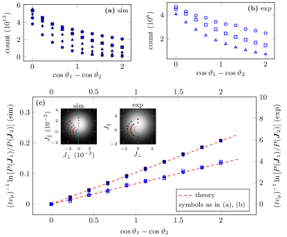
Figure 3: Upper panel: bin-counts for particle current, Eq. (15), for various $J=|\boldsymbol{J}|$, from simulation (a) and experiment (b). Lower panel: test of the vectorial fluctuation theorem, Eq. (16), using these bin-counts as proxies for $P(\boldsymbol{J})$. Insets: heatmaps for $\boldsymbol{J}$, red dots representing the bins from (a), (b).

We finally turn to the validation of the spatial fluctuation theorem, Eq. (2). In a co-rotating frame, Eq. (5) reads $\dot{\boldsymbol{r}}^{\prime}=v_{\text{p}}\boldsymbol{n}^{\prime}+\sqrt{2D}\boldsymbol{\xi}_{t}$ with $\dot{\boldsymbol{r}}^{\prime}=\boldsymbol{R}\cdot\dot{\boldsymbol{r}}$ and $\boldsymbol{R}(t)$ a time-dependent rotation matrix defined such that $\boldsymbol{n}^{\prime}\equiv\boldsymbol{R}\cdot\boldsymbol{n}$ is a constant versor arbitrarily chosen as the initial particle orientation. Self-propulsion now shows up as the constant vector $v_{\text{p}}\boldsymbol{n}^{\prime}$. Without it, the particle would simply perform isotropic diffusion, and the breaking of this spatial symmetry gives rise to the spatial fluctuation relation (2), as much as the breakdown of time-reversibility gives rise to the standard fluctuation theorem (1).

To show this, we follow the procedure leading to Eq. (11), and consider the weights

$$P[\boldsymbol{M}{{\mathcal{X}}^{\prime}}]\propto\exp{\left(-\frac{1}{4D}\int_{0}^{t}\text{d}\tau\,(\dot{\boldsymbol{r}}^{\prime}(\tau)-v_{\text{p}}\boldsymbol{M}\cdot\boldsymbol{n}^{\prime})^{2}\right)},$$

for paths $\boldsymbol{M}{{\mathcal{X}}^{\prime}}$ that only differ in the particle orientation $\boldsymbol{M}\cdot\boldsymbol{n}^{\prime}$, where $\boldsymbol{M}$ is a constant rotation matrix conserving the norm $(\boldsymbol{M}\cdot\boldsymbol{n}^{\prime})^{2}={\boldsymbol{n}^{\prime}}^{2}=1$. They are related by

$$P[{{\mathcal{X}}^{\prime}}]=P[{\boldsymbol{M}{\mathcal{X}}^{\prime}}]\exp\left(\frac{v_{\text{p}}t}{2D}{\boldsymbol{n}^{\prime}}\cdot(\boldsymbol{1}-\boldsymbol{M}^{-1})\cdot\boldsymbol{j}[{{\mathcal{X}}^{\prime}}]\right),$$ (14)

where $P[{\mathcal{X}}^{\prime}]=P[{\boldsymbol{M}{\mathcal{X}}^{\prime}}]\big{|}_{\boldsymbol{M}=\boldsymbol{1}}$, and

$$\boldsymbol{j}[{{\mathcal{X}}^{\prime}}]\equiv\frac{1}{t}\int_{0}^{t}\text{d}\tau\,\dot{\boldsymbol{r}}^{\prime}(\tau),$$ (15)

is the particle current relative to its instantaneous orientation $\boldsymbol{n}(t)$. After multiplying Eq. (14) by $\delta(\boldsymbol{j}[{\mathcal{X}}^{\prime}]-\boldsymbol{J}_{1})$ and summing over trajectories, some algebra yields

$$\frac{1}{t}\ln\frac{P(\boldsymbol{J}_{1})}{P(\boldsymbol{J}_{2})}={\frac{v_{\text{p}}}{2D}J(\cos\vartheta_{1}-\cos\vartheta_{2})}\;.$$ (16)

This spatial fluctuation relation expresses an exact symmetry between the probabilities to observe currents $\boldsymbol{J}_{i}$ of equal magnitude $J$ in different directions specified by their angles $\vartheta_{i}$ with the versor $\boldsymbol{n}^{\prime}$. Its equivalence with Eq. (2) follows from $\boldsymbol{J}_{i}\cdot\boldsymbol{n}^{\prime}=J\cos\vartheta_{i}$ by identifying $\boldsymbol{\epsilon}\equiv v_{\text{p}}\boldsymbol{n}^{\prime}\zeta/(2T_{\text{eff}})$, where one again recognizes the dissipative non-isothermal driving. Again, it is valid for all times $t$, provided that the trajectory is sampled on the diffusive time scale. And it contains the scalar fluctuation relation, Eq. (11), as the special case $\vartheta_{1}=0$, $\vartheta_{2}=\pi$, i.e., $\boldsymbol{J}_{1}=-\boldsymbol{J}_{2}=J_{\|}\boldsymbol{n}$. Figure 3c shows that it is in excellent agreement with our MD simulations and experiments.

In summary, we have verified the validity of scalar and vectorial fluctuation relations for a self-propelled colloidal particle suspended in a nonequilibrium solvent. This extends related recent work Kumar et al. (2015), which could not conclusively settle the issue for the case of an externally driven granular particle. Using a minimal Markovian model, we could recast our results in an intuitive form, revealing that the breaking of the underlying microscopic space-time symmetry is precisely quantified by the entropy production due to swimming. The latter may be written as the energy dissipated to a fictitious equilibrium bath at an effective temperature predicted by the theory of hot Brownian motion. The robustness of the established fluctuation relations against some stochasticity in the driving and the long-term memory and nonequilibrium character of the solvent fluctuations suggests that the assumptions evoked by standard derivations of fluctuation theorems are sufficient, but may actually not all be critical for their successful application.

We acknowledge funding by the Deutsche Forschungsgemeinschaft (DFG). G. F. thanks M. Polettini and C. Pérez-Espigares for discussions.

References

- Einstein (1905) A. Einstein, Annalen der Physik 322, 549 (1905).
- Franosch et al. (2011) T. Franosch, M. Grimm, M. Belushkin, F. M. Mor, G. Foffi, L. Forró, and S. Jeney, Nature 478, 85 (2011).
- Kheifets et al. (2014) S. Kheifets, A. Simha, K. Melin, T. Li, and M. G. Raizen, Science 343, 1493 (2014).
- Marchetti et al. (2013) M. C. Marchetti, J. F. Joanny, S. Ramaswamy, T. B. Liverpool, J. Prost, M. Rao, and R. A. Simha, Rev. Mod. Phys. 85, 1143 (2013).
- Ebbens and Howse (2010) S. Ebbens and J. Howse, Soft Matter 4, 726 (2010).
- Howse et al. (2007) J. R. Howse, R. A. L. Jones, A. J. Ryan, T. Gough, and R. V. R. Golestanian, Phys. Rev. Lett. 99, 048102 (2007).
- Jiang et al. (2010) H.-R. Jiang, N. Yoshinaga, and M. Sano, Phys. Rev. Lett. 105, 268302 (2010).
- Anderson (1989) L. J. Anderson, Ann. Rev. Fluid Mech. 21, 61 (1989).
- Golestanian (2012) R. Golestanian, Phys. Rev. Lett. 108, 038303 (2012).
- Theurkauff et al. (2012) I. Theurkauff, C. Cottin-Bizonne, J. Palacci, C. Ybert, and L. Bocquet, Phys. Rev. Lett. 108, 268303 (2012).
- Zheng et al. (2013) X. Zheng, B. ten Hagen, A. Kaiser, M. Wu, H. Cui, Z. Silber-Li, and H. Löwen, Phys. Rev. E 88, 032304 (2013).
- Ghosh et al. (2014) P. K. Ghosh, P. Hänggi, F. Marchesoni, and F. Nori, Phys. Rev. E 89, 062115 (2014).
- Rings et al. (2010) D. Rings, R. Schachoff, M. Selmke, F. Cichos, and K. Kroy, Phys. Rev. Lett. 105, 090604 (2010).
- Bregulla et al. (2014) A. P. Bregulla, H. Yang, and F. Cichos, ACS Nano 8, 652 (2014).
- Sekimoto (2010) K. Sekimoto, Stochastic Energetics, Lecture Notes in Physics, Vol. 799 (Springer, 2010).
- Seifert (2012) U. Seifert, Rep. Prog. Phys. 75, 126001 (2012).
- Evans et al. (1993) D. J. Evans, E. G. D. Cohen, and G. P. Morriss, Phys. Rev. Lett. 71, 2401 (1993).
- Gallavotti and Cohen (1995) G. Gallavotti and E. G. D. Cohen, Phys. Rev. Lett. 74, 2694 (1995).
- Kurchan (1998) J. Kurchan, J. Phys. A: Math. Gen 31, 3719 (1998).
- Lebowitz and Spohn (1999) J. L. Lebowitz and H. Spohn, J. Stat. Phys. 95, 333 (1999).
- Maes (1999) C. Maes, J. Stat. Phys. 95, 367 (1999).
- Seifert (2005) U. Seifert, Phys. Rev. Lett. 95, 040602 (2005).
- Hurtado et al. (2011) P. I. Hurtado, C. Pérez-Espigares, J. J. del Pozo, and P. L. Garrido, PNAS 108, 7704 (2011).
- Hurtado et al. (2014) P. I. Hurtado, C. Pérez-Espigares, J. J. del Pozo, and P. L. Garrido, J. Stat. Phys. 154, 214 (2014).
- Kumar et al. (2015) N. Kumar, H. Soni, S. Ramaswamy, and A. K. Sood, Phys. Rev. E 91, 030102 (2015).
- Joly et al. (2011) L. Joly, S. Merabia, and J.-L. Barrat, Europhys. Lett. 94 (2011).
- Falasco et al. (2014a) G. Falasco, M. V. Gnann, D. Rings, and K. Kroy, Phys. Rev. E 90, 032131 (2014a).
- Pérez-Espigares et al. (2015) C. Pérez-Espigares, F. Redig, and C. Giardiná, J Phys. A 48, 35FT01 (2015).
- Bregulla et al. (2016) A. Bregulla, A. Würger, K. Günther, M. Mertig, and F. Cichos, arXiv:1601.05888 (2016).
- Chakraborty et al. (2011) D. Chakraborty, M. V. Gnann, D. Rings, J. Glaser, F. Otto, F. Cichos, and K. Kroy, EPL (Europhysics Letters) 96, 60009 (2011).
- Schachoff et al. (2015) R. Schachoff, M. Selmke, A. Bregulla, et al., diffusion-fundamentals.org 23, 1 (2015).
- Note (1) To respect the Markovian approximation, the time derivatives have to be interpreted as discrete variations over finite time increments .
- Note (2) This formal expression should be interpreted in a discrete sense, with the integrand approximated according to the midpoint (i.e. Stratonovich) rule .
- Falasco et al. (2014b) G. Falasco, M. V. Gnann, and K. Kroy, arXiv:1406.2116 (2014b).
- Barato and Seifert (2015) A. C. Barato and U. Seifert, Phys. Rev. Lett. 114, 158101 (2015).