Effects of low anisotropy on interacting holographic and new agegraphic scalar fields models of dark energy

Abstract

A spatially homogeneous and anisotropic Bianchi type I universe is studied with the interacting holographic and new agegraphic scalar fields models of dark energy. Given, the framework of the anisotropic model, both the dynamics and potential of these scalar field models according to the evolutionary behavior of both dark energy models are reconstructed. We also investigate the cosmological evolution of interacting dark energy models, and compare it with observational data and schematic diagram. In order to do so, we focus on observational determinations of the expansion history $H(z)$. Next, we evaluate effects of anisotropy on various topics, such as evolution of the growth of perturbations in the linear regime, statefinder diagnostic, Sandage-Loeb (SL) test and distance modulus from holographic and new agegraphic dark energy models and compare the results with standard FRW and $\Lambda$CDM and $w$CDM models. Our numerical result show the effects of the interaction and anisotropy on the evolutionary behavior the new agegraphic scalar field models.

keywords: Anisotropic universe; Statefinder diagnostic; Sandage-Loeb test; Holographic dark energy; New agegraphic; Scalar field

I Introduction

Most remarkable observational discoveries in type-Ia supernovae (SN Iae) prevail that the universe has confirmed by two dark components containing dark energy (DE) and dark matter (DM) 1 ; 2 . DE, an unknown energy with large negative pressure, is employed to explain the present cosmic accelerating expansion of the universe. The simplest candidate for DE is Einstein’s cosmological constant ($\Lambda$) which is equivalent to the vacuum energy density in the universe and produces negative pressure with equation of state (EoS) parameter $\omega_{\Lambda}=-1$ since it fits the observational data. However, this model suffers from two fundamental problems, which are the fine-tuning problem and the cosmic coincidence problem.
Recently, considerable interest has been stimulated in explaining the observed DE by the holographic dark energy (HDE) model. The HDE is one of interesting DE candidates which was proposed based on the holographic principle 7 ; 8 ; 9 ; a9 . According to the holographic principle, the entropy of a system mismatch with its volume, but with its surface area 9a . The HDE was first proposed in 10 following the line of 11 where the infrared cut-off is taken to be the size of event horizon for DE. Ref. 11 purposed that the DE should obey this principle, thus its energy density has an upper limit and the fine-tuning problem for the cosmological constant is eliminated. Its framework is the black hole thermodynamics 12 and the correspondence of the UV cut-of of a quantum field theory, which gives rise to the vacuum energy, with the distance of the theory 14 ; 15 . In the following, Li 10 and Hsu 15a suggested the model $\rho_{\Lambda}=3c^{2}L^{-2}$, where $c$ is a positive constant and $L$ is the IR cut-off radius. If in a cosmological context we saturate this inequality by doing $L=H^{-1}$ 16 , where $H$ is the Hubble parameter, we obtain a model of holographic nature for the density of DE. Ref. 17 was presented a generalized and restored HDE in the braneworld context. The holographic phantom energy density grows rapidly and dominates the late time expanding phase, helping realize a cyclic universe scenario in Ref. 17a .
Another plan to explore the nature of DE, dubbed agegraphic DE (ADE), has been proposed 18 which explain the acceleration of the universe expansion with the gravitational effect in general relativity. In the ADE models the age of the universe is taken the length measure instead of the horizon distance, so the causality problem that appears in the HDE model can be avoided 18a . After introducing the ADE model by Cai 18 , a new model of agegraphic DE (NADE) was proposed in Ref. 19 , while the time scale is chosen to be the conformal time $\eta$ instead of the age of the universe i.e. $T$. The ADE go through a the difficulty to characterize the matter dominated era 19 while the NADE resolved this subject 20 . An alternative proposal for DE is the dynamical DE scenario which is often realized by scalar field mechanism. It suggests that the energy form with negative pressure is provided by a scalar field evolving down a proper potential. Some works have been investigated on the reconstruction of the scalar field in NADE models. For instance we refer to this case as agegraphic quintessence 21 ; 22 ; 28 . Also, Ref. 29 focused on the issue of age problem in the NADE model and determined the age of the universe in the NADE model by fitting the observational data.
A Bianchi type I (BI) universe, being the straightforward generalization of the flat FRW universe, is of interest because it is one of the simplest models of a non-isotropic universe exhibiting a homogeneity and spatial flatness. In this case, unlike the FRW universe which has the same scale factor for three spatial directions, a BI universe has a different scale factor for each direction. This fact introduce a non-isotropy to the system. The possible effects of anisotropy in the early universe have been investigated with BI models from different points of view 30 ; 33 ; 34 ; 35 . Therefore, we establish a correspondence between the interacting holographic and new agegraphic DE scalar field in an anisotropic universe.
The outline of this work is as follows. In the next section, a brief review of the general formulation of the field equations in a BI metric are discussed, then, interacting DE with cold DM (CDM) in a non-isotropic BI universe is studied. The Sec. III is concerned with interacting HDE with the quintessence, tachyon and K-essence scalar field in an anisotropic universe. The Sec. IV, is related to establish the correspondence between the model of interacting NADE and the quintessence, tachyon and K-essence DE in BI model. In Sec. V we study effects of anisotropy on the $H(z)$ data, Sandage-Loeb (SL) test, the statefinder diagnostic, the linear evolution of perturbations and distance modulus with both HDE and NADE models and compares it with the $\Lambda$CDM, $w$CDM and FRW models. We summarize our results in last section.

II General framework

Bianchi cosmologies are spatially homogeneous but not necessarily isotropic. Here we will consider BI cosmology. The metric of this model is given by

$$ds^{2}=dt^{2}-A^{2}(t)dx^{2}-B^{2}(t)dy^{2}-C^{2}(t)dz^{2},$$ (1)

where the metric functions, $A,B,C$, are merely functions of time, $t$. However, the underlying Lie algebra of the isometry group of the BI metrics is completely different 35a . The contribution of the interaction with the matter fields is given by the energy momentum tensor, which is defined as

$$T^{\mu}_{\nu}=diag[\rho,-\omega\rho,-\omega\rho,-\omega\rho],$$ (2)

where $\rho$ and $\omega$ represent the energy density and EoS parameter, respectively. The field equations for the axially symmetric BI metric are 36 ; 37 ; 38 :

$$3H^{2}-\sigma^{2} = \frac{1}{M_{p}^{2}}(\rho_{m}+\rho_{\Lambda}),$$ (3)

$$3H^{2}+2\dot{H}+\sigma^{2} = -\frac{1}{M_{p}^{2}}\left(p_{m}+p_{\Lambda}\right),$$ (4)

where $M_{p}^{2}=1/(8\pi G)$, $\rho_{\Lambda}$ and $p_{\Lambda}$ are the Planck mass, the energy density and pressure of DE, respectively, and $a=(ABC)^{\frac{1}{3}}$ is the scale factor, and $\sigma^{2}=1/2\sigma_{ij}\sigma^{ij}$ in which $\sigma_{ij}=u_{i,j}+\frac{1}{2}(u_{i;k}u^{k}u_{j}+u_{j;k}u^{k}u_{i})+\frac{1}{3}\theta(g_{ij}+u_{i}u_{j})$ is the shear tensor $(\sigma_{ij}u^{j}=0,\sigma^{i}_{~{}i}=0)$, which describes the rate of distortion of the matter flow, and $\theta=3H=u^{j}_{;j}$ is the scalar expansion, where $u^{j}$ is 4-velocity. In a comoving coordinate system, i.e. $(u^{i}=\delta^{i}_{0})$. From the metric Eq. (1), and considering the comoving frame, hence, the components of the average Hubble parameter and the shear tensor are given by 36

$$H = \frac{1}{3}(\frac{\dot{A}}{B}+\frac{\dot{B}}{B}+\frac{\dot{C}}{C}),$$ (5)

$$\sigma^{2} = 3H^{2}-(\frac{\dot{A}\dot{B}}{AB}+\frac{\dot{B}\dot{C}}{BC}+\frac{\dot{A}\dot{C}}{AC}).$$ (6)

By using Eq. (3), the dimensionless density parameter of BI can also be defined as usual

$$\Omega_{m} = \frac{\rho_{m}}{\rho_{cr}},\quad\Omega_{\Lambda}=\frac{\rho_{\Lambda}}{\rho_{cr}},$$ (7)

where the critical energy density is $\rho_{cr}=3M_{p}^{2}H^{2}$. Thus, the first BI equation can be rewritten as

$$\Omega_{m}+\Omega_{\Lambda}=1-\frac{\sigma^{2}}{3H^{2}}.$$ (8)

The above equation shows that the sum of the energy density parameters approaches 1 at late times if the shear tensor tend zero . Hence, at the late times the universe becomes flat,i.e. for sufficiently large time, this model predicts that the anisotropy of the universe will damp out and universe will become isotropic. By the way , in the early universe i.e. during the radiation and matter dominated era the universe have been anisotropic and the universe approaches to isotropy upon DE starts to dominate the energy density of the universe. When the isotropic is assumed, $\Omega_{m}+\Omega_{\Lambda}=1$, and the model has only one free parameter, $\Omega_{\Lambda}$. We shall take that the shear scalar can be described based on the average Hubble parameter, $\sigma^{2}=\sigma_{0}^{2}H^{2}$, where $\sigma_{0}^{2}$ is a constant. So, Eq. (8) lead to

$$\Omega_{m}+\Omega_{\Lambda}=1-\Omega_{\sigma 0},\quad~{}with~{}~{}\Omega_{\sigma 0}=\frac{\sigma_{0}^{2}}{3},$$ (9)

where $\Omega_{\sigma 0}$ is the anisotropy parameter. We assume that the DE is coupled with DM, in such way that total energy-momentum is still conserved. In the flat BI cosmology with a scale factor $a$, the continuity equations for both components are 38a

$$\dot{\rho}_{\Lambda}+3H\rho_{\Lambda}(1+\omega_{\Lambda})=-Q,$$ (10)

$$\dot{\rho}_{m}+3H\rho_{m}=Q,$$ (11)

where $\omega_{\Lambda}=p_{\Lambda}/\rho_{\Lambda}$ is the EoS parameter of the interacting DE and $Q$ is the interaction term. The case $Q>0(Q<0)$ corresponds to either DE transformation into DM and vice versa of the model. Following 14 ; 15 , we shall assume $Q=3b^{2}H(\rho_{m}+\rho_{\Lambda})$ with the coupling constant $b^{2}$. In the following, we will find a form for the function $V(\phi)$, which is able to reconstruct HDE and NADE models as following.

III HDE with Hubble radius as IR cutoff in BI model

First we will consider the size $L$ as the Hubble radius $H^{-1}$, thus the energy density for the DE becomes 7 ; 41 ; 42

$$\rho_{\Lambda}=3c^{2}M_{p}^{2}H^{2},$$ (12)

where $c^{2}$ is a constant. As it is well known, different possibilities have been tried to varying degrees of success, namely, the particle horizon 43 , the future event horizon 10 ; 14 and the Hubble horizon 16 . Hence, we set the Hubble radius as the infrared cutoff $L=H^{-1}$ 44 . The problem of taking Hubble radius,is that the DE results as pressureless, since $\rho_{\Lambda}$ scales like matter energy density $\rho_{m}$ with the scale factor $a$ as $a^{-3}$, therefore producing a decelerated expansion.But at this point our system of equations is not closed and we still have freedom to choose. In order to accelerate the universe more, we have added the interaction as well as anisotropy, as it can be seen in equation (14). This is a new model to explore the physical mechanism responsible for the current acceleration of the universe. Therefor in the present work, we have tried to compensate the effects, (due to the Hubble’s first radius that lead to a deceleration of the universe) using interaction and anisotropy. For $b^{2}=\Omega_{\sigma 0}=0$ this result is consistent with the Refs. 15a ; 42 ; 44 ; 45 ; 451 . Now by taking the time derivative of relation (12) and using the BI equation we find

$$\dot{\rho}_{\Lambda}=2\rho_{\Lambda}\frac{\dot{H}}{H}=-3\frac{Hc^{2}\rho_{\Lambda}}{1-\Omega_{\sigma 0}}(1+\omega_{\Lambda}+r),$$ (13)

where $r=\rho_{m}/\rho_{\Lambda}=(1-\Omega_{\sigma 0}-\Omega_{\Lambda})/\Omega_{\Lambda}$ is the energy density ratio. Substituting Eq. (13) into (10), the EoS parameter for interaction HDE is given by

$$\omega_{\Lambda}=-\frac{b^{2}(1-\Omega_{\sigma 0})^{2}}{c^{2}(1-c^{2}-\Omega_{\sigma 0})}.$$ (14)

This relation shows that the EoS parameter depends on the $b^{2}$, $c$ and $\Omega_{\sigma 0}$ parameters. Therefore, $\omega_{\Lambda}$ becomes a constant. In the absence of interaction between HDE and CDM, $b^{2}=0$ we have $\omega_{\Lambda}=0$, which is that matter dominant. It may be pointed out here that if one sets $\Omega_{\sigma 0}=0$, Eq. (14) reduce to that obtained for a flat FRW universe 42 .
Now, we intend to categorize our study into three types of the model, i.e. quintessence, tachyon and K-essence models in non-isotropic universe.

III.1 Quintessence reconstruction of HDE in BI

We consider a scalar field (the quintessence field) $\phi$, evolving in a potential $V(\phi)$. The density and pressure of quintessence are given by

$$\rho_{\phi} = \frac{1}{2}\dot{\phi}^{2}+V(\phi),$$ (15)

$$p_{\phi} = \frac{1}{2}\dot{\phi}^{2}-V(\phi).$$ (16)

Quintessence is usually parameterized by its equation of state $\omega_{\phi}=p_{\phi}/\rho_{\phi}$. Looking at Eqs. (15) and (16), we see immediately that $\omega_{\phi}\geq-1$. The scalar field potential and the corresponding kinetic energy of the field are obtained from Eqs. (15) and (16), which are 21

$$V(\phi) = \frac{1-\omega_{\phi}}{2}\rho_{\phi},$$ (17)

$$\dot{\phi}^{2} = (1+\omega_{\phi})\rho_{\phi},$$ (18)

where $\omega_{\phi}=p_{\phi}/\rho_{\phi}$. For the accelerated expansion of the universe, the EoS parameter for quintessence must be less than $-1/3$. By means of $\rho_{\phi}=\rho_{\Lambda}$ and $\omega_{\phi}=\omega_{\Lambda}$ and substituting Eqs. (12) and (14) into (18) one can get

$$\phi=cM_{p}\sqrt{3(1-\frac{b^{2}(1-\Omega_{\sigma 0})^{2}}{c^{2}(1-c^{2}-\Omega_{\sigma 0})})}\ln a.$$ (19)

using Eqs. (3), (7), (12) and (14) we obtain

$$\frac{\dot{H}}{H^{2}}=-\frac{3}{2}\left(1-\frac{b^{2}(1-\Omega_{\sigma 0})}{1-c^{2}-\Omega_{\sigma 0}}\right).$$ (20)

Integration of Eq. (20), the scaler field (19) can be written

$$\phi=\frac{2cM_{p}}{\sqrt{3}}\frac{\sqrt{1-\frac{b^{2}(1-\Omega_{\sigma 0})^{2}}{c^{2}(1-c^{2}-\Omega_{\sigma 0})}}}{1-\frac{b^{2}(1-\Omega_{\sigma 0})}{1-c^{2}-\Omega_{\sigma 0}}}\ln t,$$ (21)

and the potential

$$V(\phi)=\frac{2c^{2}M_{p}^{2}}{3}\bigg{(}\frac{1+\frac{b^{2}(1-\Omega_{\sigma 0})}{1-c^{2}-\Omega_{\sigma 0}}}{\left(1-\frac{b^{2}(1-\Omega_{\sigma 0})}{1-c^{2}-\Omega_{\sigma 0}}\right)^{2}}\bigg{)}exp\bigg{(}-\frac{\sqrt{3}\phi}{cM_{p}}\frac{1-\frac{b^{2}(1-\Omega_{\sigma 0})}{1-c^{2}-\Omega_{\sigma 0}}}{\sqrt{1-\frac{b^{2}(1-\Omega_{\sigma 0})^{2}}{c^{2}(1-c^{2}-\Omega_{\sigma 0})}}}\bigg{)}.$$ (22)

From the solution of (20), it is readily seen that the scale factor is $a=t^{\frac{2}{3}\left(1-\frac{b^{2}(1-\Omega_{\sigma 0})}{1-c^{2}-\Omega_{\sigma 0}}\right)^{-1}}$. It is clear that an accelerated universe, with $\ddot{a}>0$ is yielded if $b^{2}>(1-c^{2}-\Omega_{\sigma 0})/3(1-\Omega_{\sigma 0})$.

III.2 Tachyon reconstruction of HDE in BI

On the other hand, among the various candidates to explain the accelerated expansion, the rolling tachyon condensates in a class of string theories may have interesting cosmological consequences 46a ; 46b . Also, the tachyon field is originated from the D-brane action in string theory 46c ; 46d ; 46e ; 46h . It can be introduced by a simple manner as follows. In a flat BI background the energy density and the pressure density are given by 46 ; 47 ; 48

$$\rho_{T} = -T_{0}^{0}=\frac{V(\phi)}{\sqrt{1-\dot{\phi}^{2}}},$$ (23)

$$p_{T} = T_{i}^{i}=-V(\phi)\sqrt{1-\dot{\phi}^{2}}.$$ (24)

The EoS of the tachyon is given by

$$\omega_{T}=\dot{\phi}^{2}-1.$$ (25)

In the following, one can express $\phi$ in terms of $b^{2}$, $c^{2}$ and $\Omega_{\sigma 0}$. Hence, equating (14) with (25), i.e. $\omega_{\Lambda}=\omega_{T}$, gives

$$\phi(t)=\sqrt{1-\frac{b^{2}(1-\Omega_{\sigma 0})^{2}}{c^{2}(1-c^{2}-\Omega_{\sigma 0})}}t.$$ (26)

Integrating of Eq. (20) and using (26) we obtain tachyon the potential in term of the scalar field

$$V(\phi)=\frac{4M_{p}^{2}cb(1-\Omega_{\sigma 0})}{3\phi^{2}\sqrt{1-c^{2}-\Omega_{\sigma 0}}}\frac{1-\frac{b^{2}(1-\Omega_{\sigma 0})^{2}}{c^{2}(1-c^{2}-\Omega_{\sigma 0})}}{(1-\frac{b^{2}(1-\Omega_{\sigma 0})}{1-c^{2}-\Omega_{\sigma 0}})^{2}}.$$ (27)

In this case the evolution of the tachyon is as $\phi\propto t$. Tachyon potentials, which are not steep compared to $V(\phi)\propto\phi^{-2}$ lead to an accelerated expansion 49 .

III.3 K-essence reconstruction of HDE in BI

The scalar field model named K-essence is also employed to describe the observed acceleration of the cosmic expansion. This kind of models is characterized by non-canonical kinetic energy terms, and are described by a general scalar field action, which is a function of $\phi$ and $\chi=\dot{\phi}^{2}/2$, and is given by 49a ; 50

$$S=\int d^{4}x\sqrt{-g}P(\phi,\chi),$$ (28)

where $P(\phi,\chi)$ is an arbitrary function of $\phi$ and its kinetic energy $\chi$. Based on the analysis of the Lagrangian density, $‎\mathcal{L}$ ,in which,$\mathcal{L}=P,$ it can be transformed into

$$P(\phi,\chi)=f(\phi)(-\chi+\chi^{2}),$$ (29)

and the energy density in these models is given by

$$\rho(\phi,\chi)=f(\phi)(-\chi+3\chi^{2}).$$ (30)

And the EoS parameter $\omega_{K}=P(\phi,\chi)/\rho(\phi,\chi)$ is

$$\omega_{K}=\frac{\chi-1}{3\chi-1}.$$ (31)

This shows that $\omega_{K}$ does not change for fixed $\chi$. Equating $\omega_{K}=\omega_{\Lambda}$ from Eq. (14) and (31), we get

$$\chi=\frac{b^{2}(1-\Omega_{\sigma 0})^{2}+c^{2}(1-c^{2}-\Omega_{\sigma 0})}{3b^{2}(1-\Omega_{\sigma 0})^{2}+c^{2}(1-c^{2}-\Omega_{\sigma 0})}.$$ (32)

The EoS parameter in Eq. (31) diverges for $\chi=1/3$. For the case of $\chi>1/3$, the condition $\omega_{K}<-1/3$ leads to a high bound on $\chi<2/3$. The requirement of an accelerated expansion gives $1/3<\chi<2/3$ and the cosmological constant limit corresponds to $\chi=1/2$. Using Eq. (32) and $\chi=\dot{\phi}^{2}/2$, one can write the equation for the K-essence field as follows

$$\phi(t)=\sqrt{2\frac{b^{2}(1-\Omega_{\sigma 0})^{2}+c^{2}(1-c^{2}-\Omega_{\sigma 0})}{3b^{2}(1-\Omega_{\sigma 0})^{2}+c^{2}(1-c^{2}-\Omega_{\sigma 0})}}t,$$ (33)

Note that the field increases with the increment of $t$. From Eqs. (30) and (32) it can be obtained an expression for the k-essence potential $f(\phi)$ in terms of the $\phi$

$$f(\phi)=\frac{4M_{p}^{2}}{3\phi^{2}}\frac{3b^{2}(1-\Omega_{\sigma 0})^{2}+c^{2}(1-c^{2}-\Omega_{\sigma 0})}{1-c^{2}-\Omega_{\sigma 0}-b^{2}(1-\Omega_{\sigma 0})},$$ (34)

where Eq. (31) was used. From Eq. (33) we see that the kinetic energy of K-essence is not constant and is variable with cosmic time.

IV NADE with scalar field in BI model

The energy density of the NADE can be written 19 ; 20

$$\rho_{\Lambda}=\frac{3n^{2}M_{p}^{2}}{\eta^{2}},$$ (35)

where the numerical factor $3n^{2}$ has been introduced to parameterize some uncertainties, such as the species of quantum fields in the universe, or the effect of curved space-time. The conformal time is given by

$$\eta=\int\frac{dt}{a(t)}=\int\frac{da}{Ha^{2}}.$$ (36)

If $\eta$ to be a indefinite integral, the integrand give a function plus integral constant . Thus, we have $\dot{\eta}=1/a$. The energy density parameter of the NADE is now given by

$$\Omega_{\Lambda}=\frac{n^{2}}{H^{2}\eta^{2}}.$$ (37)

Taking the derivative of Eq. (35) with respect to the cosmic time and using (37) we get

$$\dot{\rho}_{\Lambda}=-2H\frac{\sqrt{\Omega_{\Lambda}}}{na}\rho_{\Lambda}.$$ (38)

Inserting this relation into (10) we obtain the EoS parameter of the interacting NADE

$$\omega_{\Lambda}=-1+\frac{2}{3na}\sqrt{\Omega_{\Lambda}}-\frac{b^{2}}{\Omega_{\Lambda}}(1-\Omega_{\sigma 0}).$$ (39)

It is important to note that when $b^{2}=0$, the interacting DE becomes trivial and Eq. (39) reduces to its respective expression in new ADE in general relativity 36 .

Figure 1: The plot shows the evolution of the EoS parameter of NADE, Eq. (39), for different the anisotropy energy density parameter $\Omega_{\sigma 0}$ and the coupling constant $b^{2}$. For both cases, we take $n=2.886$ and $\Omega_{\Lambda}^{0}=0.72$.

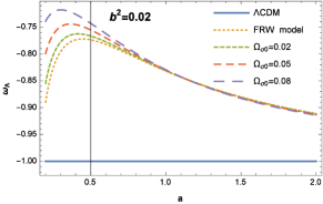
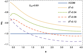
In this case ($b^{2}=0$), the present accelerated expansion of our universe can be derived only if $n>1$ 19 , in addition, from this figure we see that $\omega_{\Lambda}$ of the NADE model cannot cross the phantom divide and the universe has a quintessence region at late time; eventually, for the case of matter dominated era $\omega_{\Lambda}=-2/3$ whilst $\Omega_{\Lambda}=n^{2}a^{2}/4$ and in the radiation dominated era $\omega_{\Lambda}=-1/3$ whilst $\Omega_{\Lambda}=n^{2}a^{2}$. We test this scenario for the interaction between NADE and DM by using some observational results. For the comparison with the phenomenological interacting model, in our scenario the coupling between NADE and DM can be expressed by $b^{2}$ parameter as in the phenomenological interaction form. In fact, $b^{2}$ is within the region of the golden supernova data fitting result $b^{2}=0.00^{+0.11}_{-0.00}$ 14 and the observed CMB low $l$ data constraint 51 . In figure 1 we plot the evolution behaviors of EoS $\omega_{\Lambda}$ of DE, with respect to different choices of anisotropy energy density parameter $\Omega_{\sigma 0}$ and interaction parameter $b^{2}$ and the $\Lambda$CDM model. It clear that the EoS parameter decrease with the scale factor increase and the effect of various $\Omega_{\sigma 0}$ are negligible but as $a\rightarrow 0$, it is clear that increasing of the $\Omega_{\sigma 0}$ cause to increase the EoS parameter. Notice that in the case of $b^{2}\geq 0.08$, $\omega_{\Lambda}$ crosses the phantom divide line $\omega_{\Lambda}=-1$. Another best fit data with the NADE model is $n=2.886^{+0.084}_{-0.082}$ at the $1\sigma$ level and $n=2.886^{+0.169}_{-0.163}$ at the $2\sigma$ level 29 , $n=2.807^{+0.087}_{-0.086}(1\sigma)^{+0.176}_{-0.170}(2\sigma)$ 52 , for using the SNIa data, it is $n=2.954^{+0.264}_{-0.245}$ at $1\sigma$ Confidence Level and $n=2.716^{+0.111}_{-0.109}$ with SNIa, CMB and Large Scale Structure data 20 and for the non-flat universe $n=2.673^{+0.053+0.127+0.199}_{-0.077-0.151-0.222}$ 52a . For the $\Lambda CDM$ cosmology, $\Omega_{m0}=0.274$ is given by the WMAP five-year observations 30 . In what follows given to the Eq. (39) and its evaluations in the Fig. (1), by pick $b^{2}\neq 0$, taking account $\Omega_{m0}=0.274$ 30 , $\Omega_{\Lambda 0}=1-(\Omega_{m0}+\Omega_{\sigma 0})$, $\Omega_{\sigma 0}=0.001$, $n=2.7$ 20 and $a=1$ for the present time, Eq. (39) gives

$$\omega_{\Lambda}=-0.7905-1.3875b^{2},$$ (40)

where is clear that the phantom EoS $\omega_{\Lambda}<-1$ can be achieved by set $b^{2}>0.15$ for the coupling between NADE and CDM. In the future, where $a\rightarrow\infty$, $\omega_{\Lambda}<-1$ for $b^{2}>0$, i.e. it may be the $\omega_{\Lambda}$ crosses the phantom divide line in the presence interacting DM and DE. We can also obtain the evolution behavior of the DE. Taking the time derivative of $\Omega_{\Lambda}$ in Eq. (37) and relation $\dot{\Omega}_{\Lambda}=H\Omega_{\Lambda}^{\prime}$, give

Figure 2: (a) $\Omega_{\Lambda}$ versus $a$ for different $\Omega_{\sigma 0}$ with $b^{2}=0.02$ and $n=2.886$; (b) $\Omega_{\Lambda}$ versus $a$ for different $b^{2}$ with $\Omega_{\sigma 0}=0.001$ and $n=2.886$; (c) $\Omega_{\Lambda}$ versus $a$ for different $n$ with $\Omega_{\sigma 0}=0.001$ and $b^{2}=0.02$. The initial data is same as in Fig. (1).

$$\Omega_{\Lambda}^{\prime}=-2\Omega_{\Lambda}\left(\frac{\dot{H}}{H^{2}}+\frac{\sqrt{\Omega_{\Lambda}}}{na}\right).$$ (41)

Taking the derivative of the BI equation (3) with respect to the cosmic time, and using Eqs. (8), (10), (35) and (37), it is easy to find

$$\frac{\dot{H}}{H^{2}}=-\frac{3}{2}\bigg{(}1-b^{2}-\frac{\Omega_{\Lambda}}{1-\Omega_{\sigma 0}}+\frac{2}{3na}\frac{\Omega_{\Lambda}^{\frac{3}{2}}}{1-\Omega_{\sigma 0}}\bigg{)}.$$ (42)

Combining Eqs. (41) and (42), we have the equation of motion, a differential equation, for $\Omega_{\Lambda}$

$$\Omega_{\Lambda}^{\prime}=3\Omega_{\Lambda}\left(1-b^{2}-\frac{\Omega_{\Lambda}}{1-\Omega_{\sigma 0}}-(1-\frac{\Omega_{\Lambda}}{1-\Omega_{\sigma 0}})\frac{2\sqrt{\Omega_{\Lambda}}}{3na}\right).$$ (43)

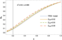
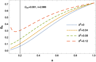
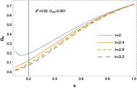
As shown in Ref. 19 , the parameters $n$ and $\Omega_{mo}$ are not independent of each other. If one takes them as free parameters, the NADE model will become confused. Therefore the initial conditions in NADE should be taken at the early times. Alike Ref. 19 proposed the initial condition for the case of ADE, $\Omega_{\Lambda}=n^{2}a^{2}/4$, at $z=1/a-1=2000$, so Eq. (43) can be numerically solved. In Fig. (2) we have depicted the evolution of $\Omega_{\Lambda}$ as a function of scale factor for various values of the free parameters for this model. Figure (2a) show the effects of the anisotropic on the evolutionary behavior the NADE model, it clear that $\Omega_{\Lambda}$ increase with increase of anisotropic parameter density at the smaller scale factor, but at the $a=1$, the effect of anisotropic parameter density is negligible,that is in agreement with observational data, i.e. the present universe is close to homogeneous and isotropic flat universe. Figures (2b) and (2c) evolution of $\Omega_{\Lambda}$ are plotted for different choices of $b^{2}$ and $n$,it is clear, the $b^{2}$ parameters increase and the $n$ decrease cause the $\Omega_{\Lambda}$ increase in the smaller scale factor but in the $a=1$, the curves are coincide, that is also in agreement with the observational data . On the other word, the evolution behaviour of $\Omega_{\Lambda}$ is as following:

(I)

For the cases of $b^{2}\neq 0.12$ and $n\neq 2$, we can see that at the early time $\Omega_{\Lambda}\rightarrow 0$, and hence the universe always behaves as an Einstein-de Sitter (EdS) cosmology, while at the late time $\Omega_{\Lambda}\rightarrow 1$, that is the NADE dominates as expected.

(II)

Finally, the plot illustrates the $\Omega_{\Lambda}$ increase with the $a$ increase.

IV.1 Quintessence reconstruction of NADE in BI

Now we suggest a correspondence between the NADE and quintessence scalar field namely, we identify $\rho_{\phi}$ to be $\rho_{\Lambda}$. Using relation $\rho_{\phi}=\rho_{\Lambda}=3M_{p}^{2}H^{2}\Omega_{\Lambda}$ and substituting Eqs. (37) and (39) into (17) and (18) one can readily find the kinetic energy term and the potential term as

$$\dot{\phi^{2}} = M_{p}^{2}H^{2}\left(\frac{2}{na}\Omega^{\frac{3}{2}}_{\Lambda}-3b^{2}(1-\Omega_{\sigma 0})\right),$$ (44)

$$V(\phi) = M_{p}^{2}H^{2}\left(3\Omega_{\Lambda}+\frac{3b^{2}}{2}(1-\Omega_{\sigma 0})-\frac{\Omega^{\frac{3}{2}}_{\Lambda}}{na}\right).$$ (45)

Figure 3: Left panel: The plot shows the evolution of the NADE quintessence scalar field, Eq. (46), for four different value of the anisotropy energy density parameter $\Omega_{\sigma 0}$. Middle panel: The plot shows the NADE quintessence potential, Eq. (45), versus the scale factor for different $\Omega_{\sigma 0}$. Right panel: The plot shows the NADE quintessence $\frac{V(\phi)}{\dot{\phi}^{2}}$, for different value of $\Omega_{\sigma 0}$. Auxiliary parameters are $\Omega_{\Lambda}^{0}=0.72$, $b^{2}=0.02$, $n=2.886$ and $\phi(1)$=0.

From definition $\dot{\phi}=H\phi^{\prime}$, one can rewrite Eq. (44) as

$$\phi^{\prime}=M_{p}\left(\frac{2}{na}\Omega^{\frac{3}{2}}_{\Lambda}-3b^{2}(1-\Omega_{\sigma 0})\right)^{\frac{1}{2}}.$$ (46)

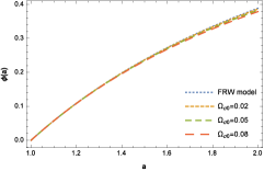
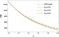
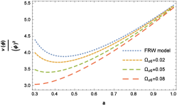
Therefore, we have established an interacting new agegraphic quintessence DE model and reconstructed the potential of the agegraphic quintessence as well as the dynamics of scalar field in an anisotropic universe. Basically, from Eqs. (43) and (46) one can derive $\phi=\phi(a)$ and then combining the result with (45) ahieve $V=V(\phi)$. Unfortunately, the analytical form of the potential in terms of the new agegraphic quintessence field cannot be determined due to the complexity of the equations involved. However, we can obtain it numerically. The evolution of the NADE quintessence scalar field and the potential $V(\phi)$ for four different values of $\Omega_{\sigma 0}$ is plotted in left and middle panel of Fig. 3. We see that the differences in the diagrams of $\phi$ are very little. It is clear, $\phi(a)$ increases and $V(\phi)$ decreases as universe expands and the curves are shifted to the smaller (bigger) values of $\phi(a)(V(\phi))$ with increasing the $\Omega_{\sigma 0}$. Also, we see from these figures that the cosmic evolution trends are quite similar for these four anisotropy energy density parameters. The evolution of $V(\phi)/\dot{\phi}^{2}$ versus $a$ is illustrated in right Fig. (3). It illustrate fraction of potential per kinetic energy increase with the $a$ increase and its magnitude increase with the $\Omega_{\sigma 0}$ decrease for the smaller $a$, that is consist of with slow-roll approximation on inflation era for the smaller $a$ at early universe.

IV.2 Tachyon reconstruction of NADE in BI

Next, we reconstruct the new agegraphic tachyon DE model, connecting the tachyon scalar field with the NADE in BI universe. Using Eqs. (37) and (39) one can easily show that the tachyon potential and kinetic energy term take the following form

$$V(\phi) = 3M_{p}^{2}H^{2}\Omega_{\Lambda}\left(1-\frac{2}{3na}\sqrt{\Omega_{\Lambda}}+\frac{b^{2}}{\Omega_{\Lambda}}(1-\Omega_{\sigma 0})\right)^{\frac{1}{2}},$$ (47)

$$\dot{\phi} = \left(\frac{2}{3na}\sqrt{\Omega_{\Lambda}}-\frac{b^{2}}{\Omega_{\Lambda}}(1-\Omega_{\sigma 0})\right)^{\frac{1}{2}}.$$ (48)

Therefore the evolution behavior of the tachyon field can be obtained by integrating the above equation

$$\phi(a)-\phi(1)=\int^{a}_{1}\frac{1}{Ha}\sqrt{\frac{2}{3na}\sqrt{\Omega_{\Lambda}}-\frac{b^{2}}{\Omega_{\Lambda}}(1-\Omega_{\sigma 0})}da,$$ (49)

Figure 4: Right panel: The evolution of the NADE tachyon scalar field, Eq. (49), for different the anisotropy energy density parameter $\Omega_{\sigma 0}$. Right panel: The NADE tachyon potential, Eq. (47), versus the scale factor for different $\Omega_{\sigma 0}$. Auxiliary parameters as in Fig. (3).

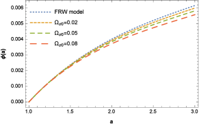
where $\Omega_{\Lambda}$ is given by Eq. (43). The evolutionary form of the tachyon field and the reconstructed tachyon potential $V(\phi)$ are plotted in Fig. (4), for different value of the anisotropy density parameter, in which again have taken $\phi(a_{0}=1)=0$ for the present time. $\Omega_{\sigma 0}$. From this figure we find out that $\phi$ increases with time while the potential $V(\phi)$ becomes steeper with decreasing $\Omega_{\sigma 0}$. This behavior is in agreement with the scaling solution $V(\phi)\propto\phi^{-2}$ obtained for the tachyon field corresponding to the power law expansion 49 . Again from right panel of Fig. (4) we find out the reconstructed scalar field has the same potential as the quintessence case.

IV.3 K-essence reconstruction of NADE in BI

Figure 5: Right panel: The K-essence scalar field as function of the scale factor for the variety values of the $\Omega_{\sigma 0}$. Left panel: The evolution of the new agegraphic K-essence kinetic energy $\chi=\dot{\phi}^{2}/2$ for different anisotropy constant $\Omega_{\sigma 0}$. Auxiliary parameters as in Fig. (3).

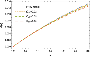
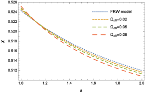
The K-essence scalar field model is also an interesting attempt to explain the origin of DE using string theory. Equating $\omega_{K}$ with the EoS parameter of NADE (39) one finds

$$\chi=\frac{2-\frac{2}{3na}\sqrt{\Omega_{\Lambda}}+\frac{b^{2}}{\Omega_{\Lambda}}(1-\Omega_{\sigma 0})}{4-\frac{2}{na}\sqrt{\Omega_{\Lambda}}+\frac{3b^{2}}{\Omega_{\Lambda}}(1-\Omega_{\sigma 0})}.$$ (50)

Using Eq. (50) and $\dot{\phi}^{2}=2\chi$, we obtain the new agegraphic K-essence scalar field as

$$\phi(a)-\phi(1)=\int^{a}_{1}\frac{1}{Ha}\sqrt{\left(\frac{4-\frac{4}{3na}\sqrt{\Omega_{\Lambda}}+\frac{2b^{2}}{\Omega_{\Lambda}}(1-\Omega_{\sigma 0})}{4-\frac{2}{na}\sqrt{\Omega_{\Lambda}}+\frac{3b^{2}}{\Omega_{\Lambda}}(1-\Omega_{\sigma 0})}\right)}da.$$ (51)

where we take $a_{0}=1$ for the present time. The evolution of the field and the reconstructed K-essence kinetic energy $\chi(\phi)$ are plotted in Fig. (5), where we have taken $\phi(a_{0}=1)=0$ for simplicity. Note that in left Fig. (5) the field increases with the increment of $a$. Obviously, the kinetic energy decreases with increasing the scale factor as shown in right panel of Fig. (5). From this figure it was observed that the range of values of the $\chi(\phi)$ is $(0.505,0.525)$ from initial to late time, which is indicates that the accelerated universe can be obtained for this interval. Note that the result of Fig. (5) is in contrast with that obtained by 52b who showed that the kinetic energy of the K-essence field increases with increasing the scale factor. This difference may come back to this fact that the K-essence field selected by 52b is a purely kinetic model in which the action (50) is independent of $\phi$.

V COSMOLOGICAL EVOLUTION OF THE INTERACTING HDE and NADE MODEL IN BI MODEL

In order to fit the model with current observational data, we consider the interacting NADE model in a flat BI universe in this section. In this case, the Hubble parameter can be written as,

$$H=H_{0}\sqrt{\frac{(1-\Omega_{\Lambda}-\Omega_{\sigma 0})X(z)}{1-\Omega_{\sigma 0}-\Omega_{\Lambda}}},$$ (52)

where $X(z)=\rho_{m}(z)/\rho_{m0}(z)$. For the case of FRW ($\Omega_{\sigma 0}=0$) which are in agreement with the respective relations obtained in 53a . Here $\Omega_{m0}$ is present value of dimensionless energy density of matter and $z$ is the redshift, $z=1/a-1$. Note that, for simplicity, in this work we disregard the contributions from baryons and radiation. For the $\Lambda$CDM model, $H(z)$ as $H=H_{0}\sqrt{\Omega_{m0}(1+z)^{3}+\Omega_{\Lambda}}$. Also, for model such as $w$CDM (with the constant EoS $w$), it is $H=H_{0}\sqrt{\Omega_{m0}(1+z)^{3}+(1-\Omega_{m0}-\Omega_{\sigma 0})(1+z)^{3(1+w)}}$. The currently preferred values of $w$ in this model is $w=-1.01\pm 0.15$ 53 .

Figure 6: Upper panel: Comparison of the observed $H(z)$, with the predictions from the NADE, HDE, $\Lambda$CDM and $w$CDM models. Middle panel the evolution of $H(z)$ versus redshift $z$ in NADE anisotropic universe for different values of parameter $\Omega_{\sigma 0}$ with $n=2.886$ and the $\Lambda$CDM models while bottom panel the evolution of $H(z)$ versus redshift $z$ for different values of parameter $n$ with $\Omega_{\sigma 0}=0.001$, by considering $H_{0}=72~{}kms^{-1}Mpc^{-1}$, $\Omega_{m0}=0.274$, $\Omega^{0}_{\Lambda}=0.69$ and $b^{2}=0.02$. For the case of $\Lambda$CDM model we take $\Omega^{0}_{\Lambda}=0.7$ and $\Omega_{m0}=0.3$, and for the $w$CDM model with $\Omega_{m0}=0.3$ and $w=-1.07$ 531 . The data points with errorbars, and theoretical lines for different DE models and the observational $H(z)$ data a53 ; b53 ; c53 ; d53 .

Figure 7: Left panel: The evolution of the shear scalar vs. $a$ for different value of $b^{2}$ and $\sigma_{0}=0.05$ 532 . Right panel: The evolution of the anisotropy parameter $\sigma/H$ with respect to the scale factor $a$ in a BI universe. It becomes almost constant during the anisotropic inflationary phase. Then it falls rapidly down to $\mathcal{O(\sigma H)}$. As shown in the legend, the interacting NADE is shown with the thin lines, and the interacting HDE with the dashed lines. The data points and error bars are estimated from Eq. (3) with a fiducial concordance $\Lambda$CDM model. The initial data is same as in Fig. (6).

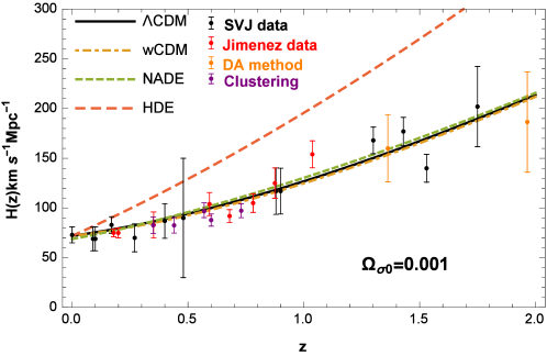
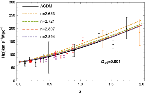
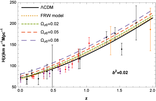
To constrain cosmological parameters we use the $H(z)$ data from SVJ a53 , DA method b53 , Jimenez c53 and Clustering d53 . These data, for the redshift range $0<z<2$, are shown in figure 6, and we find a remarkable agreement between the different measurements. The value of $H(z)$ is then directly computed by using Eq. (3). In top panel of Fig. (6), we show four models, namely, NADE, HDE, $\Lambda$CDM and $w$CDM models. We see from this figure that the cosmic evolution trends are quite similar for three models, such as, NADE, $\Lambda$CDM and $w$CDM models. So, among these four DE models, HDE with the Hubble radius $H^{-1}$ in BI is not favored by the observational data. Also from middle panel of Fig. (6), we can clearly see that for different values of $\Omega_{\sigma 0}$ the process of cosmic evolution looks quite similar, i.e., for the bigger value of the $\Omega_{\sigma 0}$ parameter, the bigger value of the Hubble expansion rate $H(z)$ is gotten. For this model, we consider, $H_{0}=72~{}kms^{-1}Mpc^{-1}$, as the value of $H_{0}=73\pm 3~{}kms^{-1}Mpc^{-1}$ from the combination WMAP 3 year estimate 54 , and the other with $H_{0}=68\pm 4~{}kms^{-1}Mpc^{-1}$ from a median statistics analysis of 461 55 . 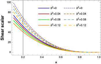The evolution of the $\sigma$ is plotted in left panel of Fig. (7). From Fig. (7), it can be observed that evolution of shear depends on the initial conditions. Signature change of shear can be seen for certain kind of coupling constant $b^{2}$. Also, the shear scalar becomes negligible at late times and $\sigma$ of NADE decreases slowly for walls compared to the HDE. Finally we have considered, the model isotropize. 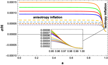The measure of the anisotropy is described by $\sigma/H$, describe the magnitude of the spacetime shear per the average expansion rate. However, as shown in right panel of Fig. (7), during the inflationary phase, we find that the effect of shear cannot become as large as the Hubble parameter and the shear decreases at the end of the inflation.
In the following, we constrain the model parameters of these DE models in BI universe by using the $H(z)$ measurements. In other words, it becomes almost constant during the anisotropic inflationary phase. Then, at the end of inflation $\sigma/H\sim\mathcal{O}(10^{-5})$.

V.1 Sandage-Loeb (SL) test

The redshift-drift observation, sometimes called the “Sandage-Loeb (SL) test”, is not only conceptually simple, but also is a direct probe of cosmic dynamic expansion, although being observationally challenging. The SL test data provide an important supplement to the other DE probes, since they are extremely helpful in breaking the existing parameter degeneracies. Ref. 53a introduced the redshift relation by a spectroscopic velocity shift $\Delta\nu$ as $\Delta\nu\equiv\Delta z/(1+z)$. By using the Hubble parameter $H(z)=-\dot{z}/(1+z)$ and Eq. (3), we obtain

$$\Delta\nu=H_{0}\Delta t_{0}\bigg{(}1-\frac{E(z)}{1+z}\bigg{)},$$ (53)

where we set $\Delta t_{0}=10$ years, and $E(z)=H(z)/H_{0}$. According to the Monte Carlo simulations, the uncertainty of $\Delta\nu$ measurements expected by CODEX can be expressed as 55a

$$\sigma^{\prime}_{\Delta\nu}=1.35(\frac{2370}{S/N})\sqrt{\frac{30}{N_{QSO}}}(\frac{5}{1+z_{QSO}})^{1.8}cm/s,$$ (54)

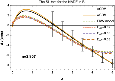
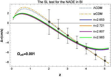
where $S/N=3000$ is the signal-to-noise ratio, $N_{QSO}=30$ is the number of observed quasars and $z_{QSO}\in[2,5]$ is their redshift. The fiducial concordance cosmological model with the parameters taken to be the best-fit ones from WMAP nine years analysis 55aa is applied to examine the capacity of future measurements of SL test to constrain the concerned models. A consistency test of the geometric and structural measurements might provide a diagnostic to the origin of the acceleration of the universe in the future. Of course, the SL test will definitely play a significant role in doing such an analysis. We will examine the SL test, and then examine effects of anisotropy and parameter of $n$ on the NADE in the SL test as shown in Fig. (8). We have chosen the fractional matter density $\Omega_{m0}=0.274$ from $\Lambda$CDM 30 and $n=2.807$ 52 . We also use the $\Lambda$CDM model as a fiducial model to perform an SL test. In left panel of Fig. (8), the parameter $n$ is fixed to be $2.807$ for the NADE model, and the parameter $\Omega_{\sigma 0}$ of the NADE model is variable while in right panel, we fix $\Omega_{\sigma 0}=0.001$ and vary $n$ for the NADE model in BI universe. Based on the parameter spaces constrained from the current data combination, the boundaries of $\Delta\nu$ could be determined by using Eq. (53). We also plot the error bars in the SL test, given by Eq. (54), on the corresponding bands, in order to make a direct comparison with the reconstructed results from the current data. From Fig. (8) we see that the NADE in BI model can be distinguished from the $\Lambda$CDM and $w$CDM models via the SL test. As we can observe $\Delta\nu$ is positive at small redshifts and becomes negative at $z\geq 1.7$. This result is reasonable with Refs. 53a ; 531 ; 56 . Clearly, for different values of $\Omega_{\sigma 0}$ and $n$, low-redshift probes cannot distinguish these different models since the required redshift is too high even for the most ambitious surveys. Beside, the amplitude and slope of the signal depend mainly on both $\Omega_{\sigma 0}$ and $n$. So, we see that the prospective SL test is very powerful to be used to constrain the NADE of BI model, and it is clearly better than the current low-redshift observations.

Figure 8: Cosmic velocity shift as function of the redshift for the NADE model with four different values of $\Omega_{\sigma 0}$ (left panel) and $n$ (right panel), the $\Lambda$CDM model with $\Omega^{0}_{\Lambda}=0.7$ and $w$CDM model with $w=-1.07$ and $\Omega_{m0}=0.3$. A time interval of 10 years has been assumed. The data points and error bars are estimated from Eq. (54) with a fiducial concordance $\Lambda$CDM model.

V.2 The statefinder diagnostic

Figure 9: Top panel: The statefinder diagrams $r(s)$ for the interacting NADE in BI model. The $\Lambda$CDM model corresponds to a fixed point $\{0,1\}$. The dots show today’s values for the statefinder parameters $(s_{0},r_{0})$. Bottom panel: Evolutionary trajectory in the $r-q$ plane for interacting NADE model in BI universe.

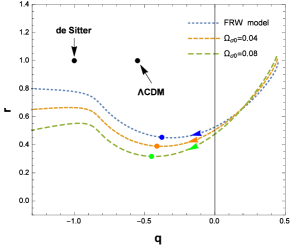
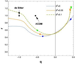
In order to achieve a strong analysis to discriminate among DE models, Sahni et al. 56a have presented a new geometrical diagnostic pair $\{r,s\}$, known as statefinder parameters, which is constructed from the scale factor and its derivatives up to the third order. The statefinder pair is a “geometrical” diagnostic in the means that it is constructed from a space-time metric directly. In the following, we consider the statefinder parameters $\{r,s\}$ 56a ; 56b ; 56c ; 56d for the present case. The ${r,s}$ parameters are given by 56a

$$r\equiv\frac{\dddot{a}}{aH^{3}},\quad~{}~{}s\equiv\frac{r-1}{3(q-\frac{1}{2})}.$$ (55)

We will soon see that it has a remarkable property for the basic flat $\Lambda$CDM BI model. The statefinder parameter $s$ is a linear combination of $r$ and $q$. In the $\{r,s\}$ plane, $s>0$ corresponds to a quintessence-like model of DE and $s<0$ corresponds to a phantom-like model of DE. In addition, other proposals on the statefinder diagnostic include varies DE models 56e ; 56g ; 56h . Then, by using the BI equation, we can obtain the following concrete expressions

$$r=1+\frac{3}{2}\Omega_{\sigma 0}+\frac{9}{2}\frac{\Omega_{\Lambda}\omega_{\Lambda}}{1-\Omega_{\sigma 0}}(1+\omega_{\Lambda}+\Omega_{\sigma 0})+\frac{9}{2}\omega_{\Lambda}b^{2}-\frac{3}{2}\frac{\Omega_{\Lambda}\omega^{\prime}_{\Lambda}}{1-\Omega_{\sigma 0}},$$ (56)

$$s=\frac{\Omega_{\sigma 0}+\frac{3\Omega_{\Lambda}\omega_{\Lambda}}{1-\Omega_{\sigma 0}}(1+\omega_{\Lambda}+\Omega_{\sigma 0})+3\omega_{\Lambda}b^{2}-\frac{\Omega_{\Lambda}\omega^{\prime}_{\Lambda}}{1-\Omega_{\sigma 0}}}{3\omega_{\Lambda}\Omega_{\Lambda}-\Omega_{\sigma 0}},$$ (57)

where $\Omega_{\Lambda}$ is given by (43) and $\omega^{\prime}_{\Lambda}=\bigg{(}\frac{\sqrt{\Omega_{\Lambda}}}{na}+\frac{3b^{2}(1-\Omega_{\sigma 0})}{\Omega_{\Lambda}}\bigg{)}\bigg{(}1-b^{2}-\frac{\Omega_{\Lambda}}{1-\Omega_{\sigma 0}}-\frac{2}{3na}(1-\frac{\Omega_{\Lambda}}{1-\Omega_{\sigma 0}})\sqrt{\Omega_{\Lambda}}\bigg{)}$. So by solving Eq. 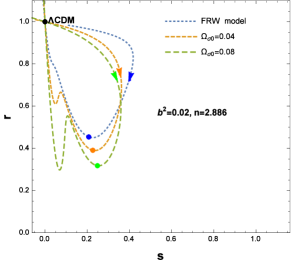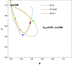(43) we can get the evolution solution of $\Omega_{\Lambda}$ and then hold all the cosmological quantities of interest and the whole dynamics of the universe. The $\{r,s\}$ evolutionary trajectory in the interacting NADE model for different values of $\Omega_{\sigma 0}$ and $b^{2}$ are shown in top panel of Fig. 9. The arrows in the diagram denote the evolution directions of the statefinder trajectories and the color dots show present-day values for the statefinder parameters. The crossing with $\Lambda$CDM occurs for this case. It can be seen that SCDM and $\Lambda$CDM models have fixed point value of statefinder pair $\{r,s\}=\{1,1\}$ and $\{r,s\}=\{1,0\}$, respectively. From Fig. 9, we can find that the the larger anisotropy parameter makes the value of $r$ smaller and the value of $s$ bigger while the the larger interaction between dark components makes the value of $s$ smaller and the value of $r$ bigger, evidently. From this figure one can observe that, in the low-redshift region, the difference between the NADE models and the $\Lambda$CDM model can be easily distinguished, which is quite different from the cases of $H(z)$ (see Fig. 6). The $r-s$ planes shows the NADE behavior, quintessence limit and will also approaches to $\Lambda$CDM behavior (see top panels of Fig. 9). As a complementarity, bottom panel of Fig. 9 shows another statefinder diagram $r-q$ evolutionary trajectory. In this case, we clearly observe that both $\Lambda$CDM ( $r=1,q=-0.55$) scenario and NADE model commence evolving from the same point in the past $r=1,q=0.5$ which corresponds to a matter dominated SCDM universe, and end their evolution at the same common point in the future $r=1,q=-1$ which corresponds to the de Sitter expansion. In Table 1 we have computed different values of $r,s,q$ for the current universe $(a=1)$ and for different choices of $b^{2}$ and $\Omega_{\sigma 0}$.
   Table 1.      Today’s values of $r$, $s$, $q$ with $n=2.886$.
Statefinder parameters $~{}~{}~{}b^{2}=0$ $~{}~{}~{}b^{2}=0.05$ $~{}~{}~{}b^{2}=0.1$ $~{}~{}~{}\Omega_{\sigma 0}=0$ $~{}~{}~{}\Omega_{\sigma 0}=0.04$ $~{}~{}~{}\Omega_{\sigma 0}=0.08$ $~{}~{}~{}~{}~{}~{}~{}~{}~{}~{}~{}~{}~{}r$ $~{}~{}~{}~{}0.433$ $~{}~{}~{}~{}0.530$ $~{}~{}~{}~{}0.745$ $~{}~{}~{}~{}0.454$ $~{}~{}~{}~{}0.391$ $~{}~{}~{}~{}0.317$ $~{}~{}~{}~{}~{}~{}~{}~{}~{}~{}~{}~{}s$ $~{}~{}~{}~{}0.222$ $~{}~{}~{}~{}0.164$ $~{}~{}~{}~{}0.079$ $~{}~{}~{}~{}0.207$ $~{}~{}~{}~{}0.226$ $~{}~{}~{}~{}0.248$ $~{}~{}~{}~{}~{}~{}~{}~{}~{}~{}~{}~{}q$ $~{}~{}-0.348$ $~{}~{}-0.423$ $~{}~{}-0.498$ $~{}~{}-0.377$ $~{}~{}-0.412$ $~{}~{}-0.451$

V.3 Linear perturbation theory

Figure 10: Time evolution of the growth factor for different value of the anisotropy energy density parameter $\Omega_{\sigma 0}$ and comparing to the $\Lambda$CDM and FRW in NADE models with $n=2.807$.

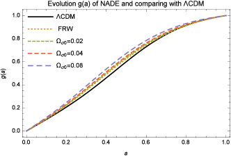
In this subsection, we study the linear growth of perturbation of non relativistic dust matter by computing the evolution of growth factor $g(a)$ in NADE model, and then compare it with the evolution of growth factor in NADE of FRW and $\Lambda$CDM models. In this case the differential equation for the evolution of $g(a)$ is given by 57 ; 58

$$g^{\prime\prime}(a)+\bigg{(}\frac{3}{a}+\frac{E^{\prime}(a)}{E(a)}\bigg{)}g^{\prime}(a)-\frac{3}{2}\frac{\Omega_{m0}}{a^{5}E^{2}(a)}g(a)=0,$$ (58)

where the prime denotes a derivative w.r.t. the scale factor. In order to study the linear growth in NADE model, using Eqs. (39), (43) and (52) for BI universe, we solve numerically Eq. (58). In addition, we solve numerically (58) for the FRW model and the $\Lambda$CDM model. To evaluate the initial conditions, since we are in the linear regime, we assume that the linear growth factor has a power law solution, $g(a)\propto a^{m}$ 57 , with $m$, to be evaluated at the initial time. We plot the evolution of $g(a)$ with respect to a function of the scale factor in Fig. (10). In the $\Lambda$CDM model, the growth factor evolves more slowly compared to the NADE in FRW universe because the expansion of the universe slows down the structure formation, but at the late time the curves to be coincide because negligible the effect of anisotropic energy density parameter . Also, in the NADE of FRW model, the growth factor evolves more slowly compared to the NADE in BI model. This behavior can be explained by taking into account the evolution of Hubble parameter in Fig. (6). Therefore the growth factor $g(a)$ for the $\Lambda$CDM and DE of FRW model will always fall behind the NADE in anisotropic universe.

V.4 Distance modulus

Finally, we consider constraints on model parameters coming from SNIa observations. Observation of SNIa does not provide standard ruler but rather gives distance modulus. This quantity is defined by 59

$$\mu_{th}(z)=5\log_{10}\frac{D_{L}(z)}{Mpc}+25.$$ (59)

The luminosity distance $D_{L}(z)$ is given by

$$D_{L}(z)=(1+z)r(z),$$ (60)

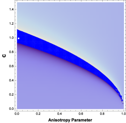
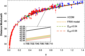
where $r(z)=\int^{z}_{0}{H^{-1}(z^{\prime})}dz^{\prime}$. In all, current SNIa data are unable to discriminate between the popular $\Lambda$CDM and our interaction model. In Fig. 11, we show the dimensional marginalized contour in the $c-\Omega_{\sigma 0}$ for the HDE model in an anisotropic universe. The fit values for the model parameters is $c=0.994^{+0.126}_{-0.065}$ at the moment time i.e. $z\rightarrow 0$. As is clear from figure 11 the parameter $c$ increases with the decreasing anisotropy parameter and this is consistent with the observed data. We can also measure $D_{L}(z)$ through the Hubble parameter by using the Eqs. (20) and (52). Figure 12 presents the distance modulus with the best fit of our model and the best fit of the $\Lambda$CDM model to the Gold and Silver SNe Ia data sets of 60 ; 61 . We add 4 SNe Ia from this current paper. From Fig. 12 we can observe the universe is accelerating expansion. In all, current data are unable to discriminate between the popular $\Lambda$CDM, FRW and our interaction models as shown in Fig. (12).

Figure 11: The constraints on the HDE model in the $c-\Omega_{\sigma 0}$ plane from the current $H(z)$ measurements in an anisotropic universe.

Figure 12: Distance modulus for the best fit model $\Omega_{m0}=0.288$, $H_{0}=72~{}km/s/Mpc$, $b^{2}=0.02$, $n=2.807$ and the $\Lambda$CDM model, $\Omega_{m0}=0.3$, $H_{0}=72~{}km/s/Mpc$ and $\Omega^{0}_{\Lambda}=0.7$. The data points are from the gold and Silver SNe Ia of 60 ; 61 .

VI Conclusion and Discussion

In this work, we have investigated the different models of cosmology in an anisotropic universe,with resemblance between their energy density to scaler fields energy density. In particular, we have reconstructed the dynamics i.e. evolution equations of these scalar field models according to the evolutionary behavior dark energy models in an anisotropic universe. Then we have reconstructed both the potentials and the kinetic energies corresponding to each model, which describe quintessence, tachyon and K-essence cosmology. We have discussed the effects of the interaction and anisotropy on the evolutionary behavior the HDE and NADE scalar field models. Our main conclusions can be summarized as follows.

• The simplest choice is the Hubble scale $L=1/H$, giving a energy density that is comparable to the present-day DE 9 ; 451 . It has been argued that an IR cutoff defined by the Hubble radius, cause the DE regard as pressureless so can not lead to an accelerated universe. We have also shown that taking into account the interaction 42 ; 45 and anisotropy terms, we are able to describe the accelerating universe. In the following, by using the Hubble radius as $L=H^{-1}$ IR cutoff, combinations of the HDE model and interacting scalar fields in anisotropic universe were implemented. We have obtained expressions for the scalar field and the potential for interacting HDE in BI model. The free parameters of cosmology have been evaluated in terms of the constants $b^{2}$, $\Omega_{\sigma 0}$ and $c^{2}$. The results of our analysis are displayed in Fig. (11). We used current observational data to constrain the HDE model. The fit values for the model parameters is $c=0.994^{+0.126}_{-0.065}$ at the moment time.

• The EoS parameter $\omega_{\Lambda}$ of the NADE model in the BI models, can cross the phantom divide line ($\omega_{\Lambda}<-1$) at the present time, provided that $b^{2}\geq 0.08$ which is compatible with the observations. By the way, the effect of various $\Omega_{\sigma 0}$ were negligible but as $a\rightarrow 0$, it was clear that decreasing of the $\Omega_{\sigma 0}$ cause to decrease the EoS parameter as shown in left panel of figure 1. The evolution of the interacting NADE density parameter $\Omega_{\Lambda}$ is depend on the anisotropy density parameter $\Omega_{\sigma 0}$.in Figure (2a) it was clear that $\Omega_{\Lambda}$ increase with increase of anisotropic parameter density at the smaller scale factor, but at the $a=1$, the effect of anisotropic parameter density is negligible,that is in agreement with observational data, i.e. the present universe is close to homogeneous and isotropic flat universe. Figures (2b) and (2c) evolution of $\Omega_{\Lambda}$ have plotted for different choices of $b^{2}$ and $n$,it is clear, the $b^{2}$ parameters increase and the $n$ decrease cause the $\Omega_{\Lambda}$ increase at the smaller scale factor but at the $a=1$, the curves are coincide, that is also in agreement with the observational data.

• The new agegraphic quintessence scalar field for a given $\Omega_{\sigma 0}$ increases with increasing the scale factor; also, the curve was shifted to the larger value of $\phi$ with decreasing $\Omega_{\sigma 0}$ as shown in left panel of Fig. (3). For a given $\Omega_{\sigma 0}$, potential $V(\phi)$ decrease with increasing the scale factor and the curve is shifted to the bigger values of $V(\phi)$ with increasing the $\Omega_{\sigma 0}$ as shown in figure 3 (middle panel). Right panel of Fig. (3) shown which the fraction of potential per kinetic energy increase with the $a$ increase and its magnitude increase with the $\Omega_{\sigma 0}$ decrease for the smaller $a$. In addition, that is consist of with slow-roll approximation on inflation era for the smaller a at early universe.

• The new agegraphic tachyon scalar field for a given $\Omega_{\sigma 0}$ behave like the new agegraphic quintessence model as shown in figure 4.

• We have evaluated the interacting NADE versions of K-essence scalar field in BI models. These results have been shown in Fig. (5). The new agegraphic K-essence scalar field for a given $\Omega_{\sigma 0}$ increases with increasing the scale factor. But its kinetic energy decreases. For a given scale factor, the new agegraphic K-essence scalar field and kinetic energy decreases with increasing $\Omega_{\sigma 0}$. Anyway, we have shown that the evolution of the NADE scalar field and kinetic energy in anisotropic universe is smaller than the evolution of the NADE scalar field and kinetic energy in FRW space time. But its potential large.

• Considering a BI model and interacting between DE and DM we have reconstructed Hubble parameter $H(z)$ (see Fig. (6)) versus the redshift $z$ and it was compared the observed expansion rate $H(z)$ with that predicted by the four DE models. We have used the SVJ, DA method and Jimenez Hubble parameter versus redshift data to constrain cosmological parameters of different DE models. The constraints are restrictive, and consistent with those determined by using type Ia supernova redshift-magnitude data. The reconstructed Hubble parameter is found to be decreasing with evolution of the universe and according to this model, the evolution of the accelerated expansion of the universe is speedy than the evolution of the isotropic model. It has seen that among different DE models, only the curve of $H(z)$ has predicted by the NADE model. So, HDE with the Hubble radius $1/H$ in BI is not favored by the observational data. We have analyzed the evolution of the shear scalar in right panel of Fig. (7), which was depending on the initial conditions and we found that there can be a change of sign in the shear. This may have some interesting implications in early universe cosmology. Furthermore, we have studied the evolution of the $\sigma/H$ as shown in left panel of figure 7. Although the shear is constant during the inflation, it can fall at the end of the inflation. Moreover, we have seen that fraction of the anisotropy of the universe to shear scaler $\sigma/H$ can decrease to $\mathcal{O}(10^{-5})$ at the end of the inflation. The Sandage-Loeb (SL) test directly measures the temporal variation of the redshift of distant quasars (QSO) Lyman-$\alpha$ absorption lines in the so-called “redshift desert” $(2\lesssim z\lesssim 5)$, which is not covered by any other cosmological observation. In Refs. 61a ; 61b ; 61c , they were performed a serious synthetic exploration of the impact of future SL test data on DE constraints. It was shown that the SL test can break the parameter degeneracies in existing DE probes and significantly improve the precision of DE constraints. In the following, we analyzed how the SL test would impact on the DE constraints from the future geometric measurements. Therefore, the SL test can be used to distinguish the NADE of FRW and NADE of BI models from the $\Lambda$CDM, the $w$CDM and it was observed that the constraints on $\Omega_{\sigma 0}$ and $n$ are very strong (see Figs. (8)). Comparing the dynamical behavior of the expansion expected in anisotropic universe with isotropic universe. The statefinder parameters are expected to be useful tools in testing interacting cosmologies that solve or at least alleviate the coincidence problem which besets many approaches to late acceleration. For this purpose, we applied the statefinder diagnostic to the NADE model with interaction in BI model. The statefinder diagrams show that the interaction between DE and DM can significantly affect the evolution of the universe and the contributions of the interaction can be diagnosed out explicitly in this method. We plot the evolutionary trajectories of this model in the statefinder parameter planes as shown in Fig. (9). The statefinder diagnostic can be performed to the NADE model in cases of different $\Omega_{\sigma 0}$ and $b^{2}$, which indicates that the value of $\Omega_{\sigma 0}$ and $b^{2}$ determines the evolution behavior and the fate of the universe. The BI NADE model can reach the $\Lambda$CDM point $\{1,0\}$ in the $r-s$ plane. In the limiting case of $b^{2}=0.02$, the trajectory of $r-s$ plane with all values of $\Omega_{\sigma 0}$ approaches to quintessence behavior as well as corresponds to $\Lambda$CDM limit as shown in top panel of Fig. (9). It is also valid for $\Omega_{\sigma 0}=0.001$ with different values of $b^{2}$. In addition, the $r-q$ plane has been used for discussion on the evolutionary property of the BI universe (see bottom panel of Fig. (9)). We have started our analysis by studying the effects of the anisotropy of the background expansion history of the growth factor and on a second step we have taken into account also the perturbations in the NADE component. We showed that the linear growth factor is sensitive to the details of the model considered. In particular, it is observed that the growth factor $g(a)$ for the $\Lambda$CDM and DE of FRW model will always fall behind the NADE in an anisotropic universe (see figure (10)). In addition to this we discuss the distance modulus with the best fit of our model and the best fit of the $\Lambda$CDM model to the Gold and Silver SNe Ia data sets of 60 ; 61 . In Fig. (12) we are able to discriminate between the $\Lambda$CDM, FRW and NADE in BI model. As a result, the NADE of BI model is consistent with current observations and the more precise cosmological observations will be taken to be the decided constraints on this model.
  Finally, we would like to mention that the aforementioned discussion in first part this work can be easily generalized to other choices of IR cut-off, namely, Ricci length scale and radius of the event horizon (for this point see also, e.g. 62 ).

Acknowledgements The authors are grateful to the referee for valuable comments and suggestions that have allowed us to improve this paper significantly.

References

- (1) A.G. Riess, A.V. Filippenko, P. Challis et al., Astron. J. 116, 1009 (1998).
- (2) S. Perlmutter, G. Aldering, G. Goldhaber, et al., Astrophys. J. 517, 565 (1999).
- (3) L. Susskind, J. Math. Phys. 36, 6377 (1995).
- (4) G.’t Hooft, Int. J. Mod. Phys. D 15, 1587 (2006).
- (5) S.D. Thomas, Phys. Rev. Lett. 89, 081301 (2002).
- (6) Q.G. Huang, M. Li, JCAP 0408, 013 (2004); Q.G. Huang, M. Li, JCAP 0503, 001 (2005).
- (7) M. Gasperini et al., Phys. Rev. D 65, 023508 (2002).
- (8) M. Li, Phys. Lett. B 603, 1 (2004).
- (9) A.G. Cohen, D.B. Kaplan, A.E. Nelson, Phys. Rev. Lett. 82, 4971 (1999).
- (10) R.C. Myers, M.J. Perry, Annals Phys. 172, 304 (1986).
- (11) B. Wang, Y. Gong and E. Abdalla, Phys. Lett. B 624, 141 (2005).
- (12) Anjan A. Sen, D. Pavón, Phys. Lett. B 664, 7 (2008).
- (13) S.D.H. Hsu, Phys. Lett. B 594, 13 (2004).
- (14) D. Pavón and W. Zimdahl, Phys. Lett. B 628, 206 (2005).
- (15) E.N. Saridakis, Phys. Lett. B 660, 138 (2008).
- (16) J. Zhang, X. Zhang and H. Liu, Eur. Phys. J. C 52, 693 (2007).
- (17) R.G. Cai, Phys. Lett. B 657, 228 (2007).
- (18) H. Wei, R.G. Cai, Eur. Phys. J. C 59, 99 (2009).
- (19) H. Wei and R.G. Cai, Phys. Lett. B 660, 113 (2008).
- (20) H. Wei and R.G. Cai, Phys. Lett. B 663, 1 (2008).
- (21) J.-P. Wu, D.-Z. Ma and Y. Ling, Phys. Lett. B 663, 152 (2008).
- (22) I.P. Neupane, Phys. Lett. B 673, 111 (2009).
- (23) J. Zhang, X. Zhang, H. Liu, Eur. Phys. J. C 54, 303 (2008).
- (24) Y.H Li, J.Z. Ma, J.L. Cui, Z. Wang and X. Zhang, Sci. China Phys. Mech. Astron. 54, 1367 (2011).
- (25) E. Komatsu et al., Astrophys. J. Suppl. Ser. 180, 330 (2009).
- (26) E. Bertschinger, Physica D 77, 354 (1994).
- (27) I. Brevik, S.V. Pettersen, Phys. Rev. D 56, 3322 (1997).
- (28) I.M. Khalatnikov and A.Yu. kamenshchik, Phys. Lett. B 553, 119 (2003).
- (29) G.F.R. Ellis, Cosmological models, (2002).
- (30) V. Fayaz, H. Hossienkhani, M. Amirabadi and N. Azimi, Astrophys. Space Sci. 353, 301 (2014).
- (31) H. Hossienkhani, A. Najafi and N. Azimi, Astrophys. Space Sci. 353, 311 (2014).
- (32) H. Hossienkhani and A. Pasqua, Astrophys. Space. Sci. 349, 39 (2014).
- (33) O. Bartolami and F. Gil, Phys. Lett. B 654, 165 (2007).
- (34) R. Bousso, Rev. Mod. Phys. 74, 825 (2002).
- (35) A. Sheykhi, Phys. Rev. D 84, 107302 (2011).
- (36) M. Cataldo, N. Cruz, S. del Campo and S. Lepe, Phys. Lett. B 509, 138 (2001).
- (37) N. Radicella and D. Pavón, JCAP 10, 005 (2010).
- (38) I. Durán, L. Parisi, Phys. Rev. D 85, 123538 (2012); W. Zimdahl and D. Pavón, Classical and Quantum Gravity 24, 22 (2006).
- (39) P. Horava, D. Minic, Phys. Rev. Lett. 85, 1610 (2000).
- (40) M. Sami, P. Chingangbam and T. Qureshi, Phys. Rev. D 66, 043530 (2002).
- (41) A. Mazumdar, S. Panda and A. Perez-Lorenzana, Nucl. Phys. B 614, 101 (2001).
- (42) A. Sen, JHEP 04, 048 (2002).
- (43) A. Sen, JHEP 07, 065 (2002).
- (44) C.P. Burgess, J.M. Cline and H. Stoica, JHEP 09, 033 (2004).
- (45) G. Dvali and H. Tye, Phys. Lett. B 450, 72 (1999).
- (46) A. Sen, JHEP 10, 008 (1999).
- (47) E.A. Bergshoeff et al., JHEP 0005, 009 (2000).
- (48) T. Padmanabhan, Phys. Rev. D 66, 021301 (2002).
- (49) E.J. Copeland, M.R. Garousi, M. Sami and S. Tsujikawa, Phys. Rev. D 71, 043003 (2005).
- (50) F. Piazza and S. Tsujikawa, JCAP 07, 004 (2004).
- (51) T. Chiba, T. Okabe, M. Yamaguchi, Phys. Rev. D 62, 023511 (2000).
- (52) B. Wang, J. Zang, Ch.Y. Lin, E. Abdalla, S. Micheletti, Nucl. Phys. B 778, 69 (2007).
- (53) M. Li, X.D. Li, S. Wang and X. Zhang, JCAP 0906, 036 (2009).
- (54) J.F. Zhang, Y.H. Li and X. Zhang, Eur. Phys. J. C 73, 2280 (2013).
- (55) A. Rozas-Fernandez, Phys. Lett. B 709, 313 (2012).
- (56) J. Zhang, L. Zhang and X. Zhang, Phys. Lett. B 691 , 11 (2010).
- (57) T.M. Davis et al., Astrophys. J. 666, 716 (2007).
- (58) R.Y. Guo and X. Zhang, Eur. Phys. C 76, 163 (2016).
- (59) J. Simon, L. Verde and R. Jimenez, Phys. Rev. D 71, 123001 (2005).
- (60) M. Moresco, Mon. Not. R. Astron. Soc. 450, L16 (2015).
- (61) R. Jimenez, Rom. Journ. Phys. 5, 863 (2012).
- (62) C. Blake et al., Mon. Not. R. Astron. Soc. 425, 405 (2012); Y.L. Li, S.Y. Li, T.J. Zhang and T.P. Li, Astrophys. J. 789, L15 (2014).
- (63) P.K. Aluri, S. Panda, M. Sharma, S. Thakur, JCAP 12, 003 (2013).
- (64) D.N. Spergel, R. Bean, O. Doré et al., Astrophys. J. Suppl. 170, 377 (2007).
- (65) J.R. Gott, M.S. Vogeley, S. Podariu and B. Ratra, Astrophys. J. 549, 1 (2001).
- (66) J. Liske, A. Grazian, E. Vanzella, M. Dessauges et al., Mon. Not. Roy. Astron. Soc. 386, 1192 (2008).
- (67) C.L. Bennett et al., Astrophys. J. Suppl. 208, 20 (2012).
- (68) X. Zhang, Phys. Rev. D 79, 103509 (2009).
- (69) V. Sahni et al., JETP Lett. 77, 201 (2003).
- (70) U. Alam, V. Sahni, T.D. Saini and A.A. Starobinsky, Mon. Not. Roy. Astron. Soc. 344, 1057 (2003).
- (71) F.Y. Wang, Z.G. Dai and S. Qi, Astronomy & Astrophysics 507, 53 (2009).
- (72) S. Chattopadhyay, Mod. Phys. Lett. A 31, 1650202 (2016).
- (73) X. Zhang, F. Q. Wu and J. Zhang, JCAP 0601, 003 (2006).
- (74) X.Z. Li, C.B. Sun and P. Xi, JCAP 0904, 015 (2009).
- (75) B.R. Chang, H.Y. Liu, L.X. Xu, C.W. Zhang and Y.L. Ping, JCAP 0701, 016 (2007).
- (76) F. Pace, L. Moscardini, R. Crittenden, M. Bartelmann, V. Pettorino, Mon. Not. Roy. Astron. Soc. 437, 547 (2014).
- (77) W.J. Percival, A & A 443, 819 (2005).
- (78) S. Wang, Y. Wang and M. Li, (2016), arXiv:1612.00345v1.
- (79) A.G. Riess, W.H. Press, R.P. Kirshner, ApJ, 473, 588 (1996).
- (80) A.G. Riess, L.G. Strolger, S. Casertano et al., ApJ, 659, 98 (2007).
- (81) J.J. Geng, J.F. Zhang and X. Zhang, J. Cosmol. Astropart. Phys. 07, 006 (2014).
- (82) J.J. Geng, J.F. Zhang and X. Zhang, J. Cosmol. Astropart. Phys. 12, 018 (2014).
- (83) J.J. Geng, Y.H. Li, J.F. Zhang and X. Zhang, Eur. Phys. J. C 75, 8, 356 (2015).
- (84) V. Fayaz, H. Hossienkhani and A. Jafari, Eur. Phys. J. Plus 132, 193 (2017).