A Streaming Algorithm for Crowdsourced Data Classification

Abstract

We propose a streaming algorithm for the binary classification of data based on crowdsourcing. The algorithm learns the competence of each labeller by comparing her labels to those of other labellers on the same tasks and uses this information to minimize the prediction error rate on each task. We provide performance guarantees of our algorithm for a fixed population of independent labellers. In particular, we show that our algorithm is optimal in the sense that the cumulative regret compared to the optimal decision with known labeller error probabilities is finite, independently of the number of tasks to label. The complexity of the algorithm is linear in the number of labellers and the number of tasks, up to some logarithmic factors. Numerical experiments illustrate the performance of our algorithm compared to existing algorithms, including simple majority voting and expectation-maximization algorithms, on both synthetic and real datasets.

Keywords: Crowdsourcing; data classification; streaming algorithms; statistics; machine learning.

1 Introduction

The performance of most machine learning techniques, and in particular data classification, strongly depends on the quality of the labeled data used in the initial training phase. A common way to label new datasets is through crowdsourcing: many people are asked to label data, typically texts or images, in exchange of some low payment. Of course, crowdsourcing is prone to errors due to the difficulty of some classification tasks, the low payment per task and the repetitive nature of the job. Some labellers may even introduce errors on purpose. Thus it is essential to assign the same classification task to several labellers and to learn the competence of each labeller through her past activity so as to minimize the overall error rate and to improve the quality of the labeled dataset.

Learning the competence of each labeller is a tough problem because the true label of each task, the so-called “ground-truth”, is unknown (it is precisely the objective of crowdsourcing to guess the true label). Thus the competence of each labeller must be inferred from the comparison of her labels on some set of tasks with those of other labellers on the same set of tasks.

In this paper, we consider binary labels and propose a novel algorithm for learning the error probability of each labeller based on the correlations of the labels. Specifically, we infer the error probabilities of the labellers from their agreement rates, that is for each labeller the proportion of other labellers whom agree with her. A key feature of this agreement-based algorithm is its streaming nature: it is not necessary to store the labels of all tasks, which may be expensive for large datasets. Tasks can be classified on the fly, which simplifies the implementation of the algorithm. The algorithm can also be easily adapted to non-stationary environments where the labeller error probabilities evolve over time, due for instance to the self-improvement of the labellers or to changes in the type of data to label. The complexity of the algorithm is linear, up to some logarithmic factor.

We provide performance guarantees of our algorithm for a fixed population of labellers, assuming each labeller works on each task with some fixed probability and provides the correct label with some other fixed, unknown probability, independently of the other labellers. In particular, we show that our algorithm is optimal in terms of cumulative regret, namely the number of labels that are different from those given by the optimal decision, assuming the labeller error rates are perfectly known, is finite, independently of the number of tasks. We also propose a modification of the algorithm suitable for non-stationary environments and provide performance guarantees in this case as well. Finally, we compare the performance of our algorithm to those of existing algorithms, including simple majority voting and expectation-maximization algorithms, through numerical experiments using both synthetic and real datasets.

The rest of the paper is organized as follows. We present the related work in the next section. We then describe the model and the proposed algorithm. Section 4 is devoted to the performance analysis and Section 5 to the adaptation of the algorithm to non-stationary environments. The numerical experiments are presented in Section 6. Section 7 concludes the paper.

2 Related Work

The first problems of data classification using independent labellers appeared in the medical context, where each label refers to the state of a patient (e.g., sick or sane) and the labellers are clinicians. In [4], Dawid and Skene proposed an expectation-maximization (EM) algorithm, admitting that the accuracy of the estimate was unknown. Several versions and extensions of this algorithm have since been proposed and tested in various settings [8, 18, 1, 16, 12], without any significant progress on the theoretical side. Performance guarantees have been provided only recently for an improved version of the algorithm relying on spectral methods in the initialization phase [22].

A number of Bayesian techniques have also been proposed and applied to this problem, see [16, 20, 9, 12, 11, 10] and references therein. Of particular interest is the belief-propagation (BP) algorithm of Karger, Oh and Shah [9], which is provably order-optimal in terms of the number of labellers required per task for any given target error rate, in the limit of an infinite number of tasks and an infinite population of labellers.

Another family of algorithms is based on the spectral analysis of some matrix representing the correlations between tasks or labellers. Gosh, Kale and McAfee [5] work on the task-task matrix whose entries correspond to the number of labellers having labeled two tasks in the same manner, while Dalvi et al. [3] work on the labeller-labeller matrix whose entries correspond to the number of tasks labeled in the same manner by two labellers. Both obtain performance guarantees by the perturbation analysis of the top eigenvector of the corresponding expected matrix. The BP algorithm of Karger, Oh and Shah is in fact closely related to these spectral algorithms: their message-passing scheme is very similar to the power-iteration method applied to the task-labeller matrix, as observed in [9].

A recent paper proposes an algorithm based on the notion of minimax conditional entropy [23], based on some probabilistic model jointly parameterized by the labeller ability and the task difficulty. The algorithm is evaluated through numerical experiments on real datasets only; no theoretical results are provided on the performance and the complexity of the algorithm.

All these algorithms require the storage of all labels in memory. To our knowledge, the only streaming algorithm that has been proposed for crowdsourced data classification is the recursive EM algorithm of Wang et al. [19], for which no performance guarantees are available.

Some authors consider slightly different versions of our problem. Ho et al. [7, 6] assume that the ground truth is known for some tasks and use the corresponding data to learn the competence of the labellers in the exploration phase and to assign tasks optimally in the exploitation phase. Liu and Liu [13] also look for the optimal task assignment but without the knowledge of any true label: an iterative algorithm similar to EM algorithms is used to infer the competence of each labeller, yielding a cumulative regret in $O(\log^{2}t)$ for $t$ tasks compared to the optimal decision. Finally, some authors seek to rank the labellers with respect to their error rates, an information which is useful for task assignment but not easy to exploit for data classification itself [2, 15].

3 Model and Algorithm

3.1 Model

Consider $n$ labellers, for some integer $n>2$. Each task consists in determining the answer to a binary question. The answer to task $t$, the “ground-truth”, is denoted by $G(t)\in\{+1,-1\}$. We assume that the random variables $G(1),G(2),\ldots$ are i.i.d. and centered, so that there is no bias towards one of the answers.

Each labeller provides an answer with probability $\alpha\in(0,1]$. When labeller $i\in\{1,...,n\}$ provides an answer, this answer is incorrect with probability $p_{i}\in[0,1]$, independently of other labellers: $p_{i}$ is the error rate of labeller $i$, with $p_{i}=0$ if labeller $i$ is perfectly accurate, $p_{i}=\frac{1}{2}$ if labeller $i$ is non-informative and $p_{i}=1$ if labeller $i$ always gives the wrong answer. We denote by $p$ the vector $(p_{1},\ldots,p_{n})$.

Denote by $X_{i}(t)\in\{-1,0,1\}$ the output of labeller $i$ for task $t$, where the output $0$ corresponds to the absence of an answer. We have:

$$X_{i}(t)=\begin{cases}G(t)&\text{ w.p. }\;\;\;\alpha(1-p_{i}),\\ -G(t)&\text{ w.p. }\;\;\;\alpha p_{i},\\ 0&\text{ w.p. }\;\;\;1-\alpha.\end{cases}$$

Since the labellers are independent, the random variables $X_{1}(t),...,X_{n}(t)$ are independent given $G(t)$, for each task $t$. We denote by $X(t)$ the corresponding vector. The goal is to estimate the ground-truth $G(t)$ as accurately as possible by designing an estimator ${\hat{G}}(t)$ that minimizes the error probability $\mathbb{P}({\hat{G}}(t)\neq G(t))$. The estimator ${\hat{G}}(t)$ is adaptive and may be a function of $X(1),...,X(t)$ and the parameter $\alpha$ (which is assumed known), but cannot depend on $p$ which is a latent parameter in our setting.

3.2 Weighted majority vote

It is well-known that, given $p$ and $\alpha=1$, an optimal estimator of ${G}(t)$ is the weighted majority vote [14, 17], namely

$$\hat{G}(t)={\bf 1}\{W(t)>0\}-{\bf 1}\{W(t)<0\}+Z{\bf 1}\{W(t)=0\},$$ (1)

where $W(t)=\frac{1}{n}\sum_{i=1}^{n}w_{i}X_{i}(t)$, $w_{i}=\log(1/{p_{i}}-1)$ is the weight of labeller $i$ (possibly infinite), and $Z$ is a Bernoulli random variable of parameter $\frac{1}{2}$ over $\{+1,-1\}$ (for random tie-breaking). We provide a proof that accounts for the fact that labellers may not provide an answer for each task.

Proposition 1

Assuming $p$ is known, the estimator (1) is an optimal estimator of $G(t)$.

Proof. Finding an optimal estimator of ${G}(t)$ amounts to finding an optimal statistical test between hypotheses $\{G(t)=+1\}$ and $\{G(t)=-1\}$, under a symmetry constraint so that type I and type II error probability are equal. Consider a sample $X(t)=x\in\{-1,0,1\}^{n}$ and denote by $L^{+}(x)$ and $L^{-}(x)$ its likelihood under hypotheses $\{G(t)=+1\}$ and $\{G(t)=-1\}$, respectively. We have

$$L^{+}(x) =\prod_{i=1}^{n}(\alpha p_{i})^{{\bf 1}\{x_{i}=-1\}}(\alpha(1-p_{i}))^{{\bf 1}\{x_{i}=1\}}(1-\alpha)^{{\bf 1}\{x_{i}=0\}},$$

$$L^{-}(x) =\prod_{i=1}^{n}(\alpha p_{i})^{{\bf 1}\{x_{i}=1\}}(\alpha(1-p_{i}))^{{\bf 1}\{x_{i}=-1\}}(1-\alpha)^{{\bf 1}\{x_{i}=0\}}.$$

We deduce the log-likelihood ratio,

$$\log\left(\frac{L^{+}(x)}{L^{-}(x)}\right)=\sum_{i=1}^{n}w_{i}x_{i}=w^{T}x.$$

By the Neyman-Pearson theorem, for any level of significance, there exists $a$ and $b$ such that the uniformly most powerful test for that level is:

$${\bf 1}\{w^{T}x>a\}-{\bf 1}\{w^{T}x<a\}+Z{\bf 1}\{w^{T}x=a\},$$

where $Z$ is a Bernoulli random variable of parameter $b$ over $\{+1,-1\}$. By symmetry, we must have $a=0$ and $b=\frac{1}{2}$, which is the announced result. $\Box$

This result shows that estimating the true answer $G(t)$ reduces to estimating the latent parameter $p$, which is the focus of the paper.

3.3 Average error probability

A critical parameter for the estimation of $p$ is the average error probability,

$$q=\frac{1}{n}\sum_{i=1}^{n}p_{i}.$$

We assume the following throughout the paper:

Assumption 1

We have $q<\frac{1}{2}-\frac{1}{n}$.

This assumption is essential. First, it is necessary to assume that $q<\frac{1}{2}$, i.e., labellers say “mostly the truth”. Indeed, the transformation $p\mapsto 1-2p$ does not change the distribution of $X(t)$, meaning that the parameters $p$ and $1-2p$ are statistically indistinguishable: it is the assumption $q<\frac{1}{2}$ that breaks the symmetry of the problem and allows one to distinguish between true and false answers.

Next, the accurate estimation of $p$ requires that there is enough correlation between the labellers’ answers. Taking $p=(0,\frac{1}{2},\ldots,\frac{1}{2})$ for instance, the mean error rate is $q=\frac{1}{2}-\frac{1}{2n}$ but the estimation of $p$ is impossible since any permutation of the indices of $p$ lets the distribution of $X(t)$ unchanged. For $p=(0,0,\frac{1}{2},\ldots,\frac{1}{2})$, the average error probability becomes $q=\frac{1}{2}-\frac{1}{n}$, the maximum value allowed by Assumption 1, and the estimation becomes feasible.

3.4 Prediction error rate

Before moving to the estimation of $p$, we give upper bounds on the prediction error rate, that is the probability that $\hat{G}(t)\neq G(t)$, given some estimator $\hat{p}$ of $p$.

First consider the case $\hat{p}=(\frac{1}{2},\ldots,\frac{1}{2})$, which is a natural choice when nothing is known about $p$. The corresponding weights $\hat{w}_{1},\ldots,\hat{w}_{n}$ are then equal and the estimator $\hat{G}(t)$ boils down to majority voting. We get

$$\mathbb{P}({\hat{G}}(t)\neq G(t))\leq\mathbb{P}(\sum_{i=1}^{n}X_{i}(t)\leq 0|G(t)=1)\leq\exp\left({-\frac{n}{2}(\alpha(1-2q))^{2}}\right),$$

the second inequality following from Hoeffding’s inequality. For any fixed $q<1/2$, the prediction error probability decreases exponentially fast with $n$.

Now let $\hat{p}\in(0,1)^{n}$. The corresponding weights $\hat{w}_{1},\ldots,\hat{w}_{n}$ are finite and the estimate $\hat{G}(t)$ follows from weighted majority voting. Again,

$$\mathbb{P}({\hat{G}}(t)\neq G(t))\leq\mathbb{P}\left(\sum_{i=1}^{n}\hat{w}_{i}X_{i}(t)\leq 0|G(t)=1\right)\leq\exp\left({-\frac{1}{2}\frac{(\alpha\sum_{i=1}^{n}\hat{w}_{i}(1-2p_{i}))^{2}}{\sum_{i=1}^{n}\hat{w}_{i}^{2}}}\right),$$

the second inequality following from Hoeffding’s inequality.

Consider for instance the “hammer-spammer” model where $\alpha=1$ and $p=(0,\ldots,0,\frac{1}{2},\ldots,\frac{1}{2})$, i.e., half of the labellers always tell the truth while the other half always provide random answers. We obtain upper bounds on the prediction error rate equal to $e^{-n/8}$ for $\hat{p}=(\frac{1}{2},\ldots,\frac{1}{2})$ and $e^{-n/4}$ for $\hat{p}\to p$. Taking $n=20$ for instance, we obtain respective bounds on the prediction error rate equal to $e^{-2.5}\approx 0.08$ and $e^{-5}\approx 0.007$: assuming these bounds are tight, this means that the accurate estimation of $p$ may decrease the prediction error rate by an order of magnitude.

3.5 Agreement-based algorithm

Maximum likelihood

We are interested in designing an estimator of $p$ which has low complexity and may be implemented in a streaming fashion. The most natural way of estimating $p$ would be to consider the true answers $G(1),...,G(t)$ as latent parameters, and to calculate the maximum likelihood estimate of $p$ given the observations $X(1),...,X(t)$. The likelihood of a sample $x(1),...,x(t)$ given $G(1)=g(1),\ldots,G(t)=g(t)$ is

$$\prod_{s=1}^{t}\left(L^{+}(x(s)){\bf 1}\{g(s)=+1\}+L^{-}(x(s)){\bf 1}\{g(s)=-1\}\right).$$

This approach has two drawbacks. First, there is no simple sufficient statistic, so that one must store the whole sample $x(1),...,x(t)$, which incurs a memory space of ${O}(nt)$ and prevents any implementation through a streaming algorithm. Second, the likelihood is expressed as a product of sums, so that the maximum likelihood estimator is hard to compute, and one must rely on iterative methods such as EM.

Agreement rates

We propose instead to estimate $p$ through the vector $a$ of agreement rates. We define the agreement rate of labeller $i$ as the average proportion of other labellers whom agree with $i$, i.e.,

$$a_{i} =\frac{1}{n-1}\sum_{j\neq i}\mathbb{P}(X_{i}(t)X_{j}(t)=1|X_{i}(t)X_{j}(t)\neq 0),$$

$$=\frac{1}{n-1}\sum_{j\neq i}(p_{i}p_{j}+(1-p_{i})(1-p_{j})).$$ (2)

Observe that $a_{i}\in[0,1]$, with $a_{i}=0$ if labeller $i$ never agrees with the other labellers and $a_{i}=1$ if labeller $i$ always agrees with the other labellers.

Using the average error probability $q$, we get

$$a_{i}=\frac{1}{n-1}(p_{i}(nq-p_{i})+(1-p_{i})(n-1-nq+p_{i})),$$

so that

$$2p_{i}^{2}-2p_{i}(n(q-\frac{1}{2})+1)+nq-(1-a_{i})(n-1)=0.$$ (3)

For any fixed $a_{i}$ and $q$, we see that $p_{i}$ is a solution to a quadratic equation; in view of Assumption 1, this is the unique non-negative solution to this equation.

Fixed-point equation

For any $u\in[0,1]^{n}$ and $v\in\mathbb{R}$, let

$$\delta_{i}(u,v)=v+4\frac{n-1}{n^{2}}(1-2u_{i}).$$

Observe that this is the discriminant of the quadratic equation (3) for $u=a$ and $v=(2q-1)^{2}$. It is non-negative whenever $v\geq v_{0}(u)$, with

$$v_{0}(u)=\max(4\frac{n-1}{n^{2}}\max_{i=1,\ldots,n}(2u_{i}-1),0).$$

Define the function $f$ by

$$\forall u,\forall v\geq v_{0}(u),\quad f(u,v)=\left(\frac{1}{n-2}\sum_{i=1}^{n}\sqrt{\delta_{i}(u,v)}\right)^{2}.$$

Proposition 2

The mapping $v\mapsto f(u,v)-v$ is strictly increasing over $[v_{0}(u),+\infty)$.

Proof. For any $u\in[0,1]^{n}$ and $v>v_{0}(u)$, we have $\delta_{i}(u,v)>0$ for all $i$, so that $v\mapsto f(u,v)$ is differentiable and its partial derivative is:

$$\frac{\partial f}{\partial v}(u,v) =\frac{1}{(n-2)^{2}}\left(\sum_{i=1}^{n}\sqrt{\delta_{i}(u,v)}\right)\left(\sum_{i=1}^{n}\frac{1}{\sqrt{\delta_{i}(u,v)}}\right).$$

Using Fact 1, we obtain

$$\frac{\partial f}{\partial v}(u,v)\geq\frac{n^{2}}{(n-2)^{2}}>1.$$

$\Box$

Fact 1

For any positive real numbers $\chi_{1},\ldots,\chi_{n}$,

$$\left(\sum_{i=1}^{n}{\chi_{i}}\right)\left(\sum_{i=1}^{n}\frac{1}{{\chi_{i}}}\right)\geq n^{2}.$$

Proof. This is another way to express the fact that the arithmetic mean is greater than or equal to the harmonic mean. $\Box$

In view of Proposition 2, there is at most one solution to the fixed-point equation $v=f(u,v)$ over $[v_{0}(u),+\infty)$, and this solution $v(u)$ exists if and only if

$$f(u,v_{0}(u))\leq v_{0}(u).$$ (4)

Moreover, the solution can be found by a simple binary search algorithm.

Now let $g$ be the function defined by

$$\forall u,\forall v\geq v_{0}(u),\quad g_{i}(u,v)=\frac{1}{2}+\frac{n}{4}\left(\sqrt{\delta_{i}(u,v)}-\sqrt{v}\right).$$

For any $u$ that satisfies (4), we define $\phi(u)=g(u,v(u)).$

Proposition 3

The unique solution to the fixed-point equation $v=f(a,v)$ is $v(a)=(1-2q)^{2}$. Moreover, we have $v(a)>v_{0}(a)$ and $p=\phi(a)$.

Proof. Let $v=(1-2q)^{2}$. It can be readily verified from (3) that $p_{i}=g_{i}(a,v)$. It then follows from Assumption 1 that $\delta_{i}(a,v)>0$ and thus $v>v_{0}(a)$. Moreover,

$$v=\left(1-\frac{2}{n}\sum_{i=1}^{n}p_{i}\right)^{2}=\left(1-\frac{2}{n}\sum_{i=1}^{n}g_{i}(a,v)\right)^{2}=\left(\frac{1}{2}\sum_{i=1}^{n}\sqrt{\delta_{i}(a,v)}-\frac{n}{2}\sqrt{v}\right)^{2},$$

so that, taking the square root of both terms, $v$ satisfies the fixed-point equation $v=f(a,v)$. This shows that $v(a)=v$ and $p=g(a,v(a))=\phi(a)$. $\Box$

Estimator

Proposition 3 suggests that it is sufficient to estimate $a$ in order to retrieve $p$. We propose the following estimate of $a$,

$${\hat{a}}_{i}(t)=\frac{t-1}{t}{\hat{a}}_{i}(t-1)+\frac{1}{t(n-1)\alpha^{2}}\sum_{j\neq i}{{\bf 1}\{X_{i}(t)X_{j}(t)=1\}},$$ (5)

with ${\hat{a}}_{i}(0)=0$ for all $i=1,\ldots,n$. Note that

$${\hat{a}}_{i}(t)=\frac{1}{t(n-1)\alpha^{2}}\sum_{s=1}^{t}\sum_{j\neq i}{{\bf 1}\{X_{i}(s)X_{j}(s)=1\}},$$ (6)

so that ${\hat{a}}_{i}(t)$ is the empirical average of the number of labellers whom agree with $i$ for tasks $1,\ldots,t$. We use the definition (5) to highlight the fact that ${\hat{a}}(t)$ can be computed in a streaming fashion.

The time complexity of the update (5) is $O(n^{2})$ per task. Using the fact that ${\bf 1}\{x=1\}=\frac{1}{2}(x+|x|)$ over $\{-1,0,1\}$, we can in fact update the estimator $\hat{a}(t)$ as follows,

$${\hat{a}}_{i}(t)=\frac{t-1}{t}{\hat{a}}_{i}(t-1)+\frac{X_{i}(t)S(t)+|X_{i}(t)|(|N(t)|-2)}{2t(n-1)\alpha^{2}},$$

where $S(t)=\sum_{j=1}^{n}X_{j}(t)$ is the sum of the labels of task $t$ and $N(t)=\sum_{j=1}^{n}|X_{j}(t)|$ is the total number of actual labellers for task $t$. The time complexity of the update is then $O(n)$ per task.

Algorithm

Given this estimation of the vector $a$ of agreement rates, our estimation of the vector ${p}$ of error probabilities is

• ${\hat{p}}(t)=\phi(\hat{a}(t))$ if the fixed-point equation $v=f({\hat{a}}(t),v)$ has a unique solution,

• ${\hat{p}}(t)=(\frac{1}{2},...,\frac{1}{2})$ otherwise.

We denote by $\hat{w}(t)$ the corresponding weight vector, with $\hat{w}_{i}(t)=\log(1/\hat{p}_{i}(t)-1)$ for all $i=1,\ldots,n$. These weights inferred from tasks $1,\ldots,t$ are used to label task $t+1$ according to weighted majority vote, as defined by (1). We refer to this algorithm as the agreement-based (AB) algorithm.

4 Performance guarantees

In this section, we provide performance guarantees for the AB algorithm, both in terms of statistical error and computational complexity, and show that its cumulative regret compared to an oracle that knows the latent parameter $p$ is finite, for any number of tasks.

4.1 Accuracy of the estimation

Let $\gamma=v(a)-v_{0}(a)$. This is a fixed parameter of the model. Observe that $\gamma\in(0,1]$ in view of Proposition 3 and the fact that $v(a)=(1-2q)^{2}\leq 1$. Theorem 1, proved in the Appendix, gives a concentration inequality on the estimation error at time $t$ (that is, after having processed tasks $1,\ldots,t$). We denote by $||\cdot||_{\infty}$ the $\ell_{\infty}$ norm in $\mathbb{R}^{n}$.

Theorem 1

For any $\varepsilon\in(0,\frac{1}{20}]$,

$$\mathbb{P}(||\hat{p}(t)-p||_{\infty}\geq\varepsilon) \leq 2n\exp\left(-\frac{\gamma^{3}\alpha^{4}}{8}t\varepsilon^{2}\right).$$

Corollary 1

The estimation error is of order

$$||\hat{p}(t)-p||_{\infty} =O\left(\frac{1}{\gamma^{3\over 2}\alpha^{2}}\sqrt{\log n\over t}\right).$$

As shown by Corollary 1, Theorem 1 yields the error rate of our algorithm in the regime where $q$ and $\alpha$ are fixed and $t/\log n\to\infty$, but is much stronger than what one may obtain through an asymptotic analysis. Indeed, for any values of $n$ and $t$, Theorem 1 shows that the mean estimation error exhibits sub-Gaussian concentration, and directly yields confidence regions for the vector ${\hat{p}}(t)$. This may useful for instance in a slightly different setting where the number of samples $nt$ is not fixed, and one must find a stopping criterion ensuring that the estimation error is below some target accuracy. An example of this setting arises when one attempts to identify the best $k<n$ labellers under some constraint on the number of samples.

4.2 Complexity

In order to calculate ${\hat{p}}(t)$, we only need to store the value of ${\hat{a}}(t)$, which requires $O(n)$ memory space. Further, we have seen that the update of $\hat{a}(t)$ requires $O(n)$ operations. For any $\epsilon(t)>0$ computing the fixed point $v(\hat{a}(t))$ (using a binary search) up to accuracy $\epsilon(t)$ requires $O(n\log(1/\epsilon(t)))$ operations. The accuracy of our estimate is $O(\sqrt{\log n/t})$ (omitting the factors $\alpha$ and $\gamma$), so that one should use $\epsilon(t)=O(\sqrt{\log n/t})$. The time complexity of our algorithm is then $O(n\log t)$. It is noted that any estimator of $p$ requires at least $O(n)$ space and $O(n)$ time, since one has to store at least one statistic per labeller, and each component of $p$ must be estimated. Therefore the complexity of the AB algorithm is optimal (up to logarithmic factors) in both time and space.

4.3 Regret

The regret is a performance metric that allows one to compare any algorithm to the optimal decision knowing the latent parameter $p$, given by some oracle. We define two notions of regret. The simple regret is the difference between the prediction error rate of our algorithm and that of the optimal decision for task $t$. By Proposition 1, the optimal decision follows from weighted majority voting with weights $w$ given by the oracle; we denote by ${G^{\star}}(t)$ the corresponding output for task $t$. The simple regret is then

$$r(t)=\mathbb{P}({\hat{G}}(t)\neq G(t))-\mathbb{P}({G^{\star}}(t)\neq G(t)).$$

The second performance criterion is the cumulative regret, $R(t)=\sum_{s=1}^{t}r(s)$, that is the difference between the expected number of errors done by our algorithm and that of the optimal decision, for tasks $1,\ldots,t$.

Let $\eta=\min_{i}p_{i}(1-p_{i})$ and $\lambda=\min_{x\in\{-1,0,1\}^{n}:w^{T}x\neq 0}|w^{T}x|.$ The following result, proved in the Appendix, shows that the cumulative regret of the AB algorithm is finite.

Theorem 2

Assume that $\eta>0$. We have

$$r(t) \leq 2n\exp\left({-\frac{\gamma^{3}\alpha^{4}c^{2}}{8}t}\right),$$

with $c=\frac{1}{4}\min(\lambda\eta,\frac{1}{5})$, and

$$R(t)\leq\frac{16n}{\gamma^{3}\alpha^{4}c^{2}}.$$

5 Non-Stationary Environment

We have so far assumed a stationary environment so that the latent parameters $p$ stay constant over time. We shall see that, due to its streaming nature, our algorithm is also well-suited to non-stationary environments. In practice, the vector of error probabilities $p$ may vary over time due to several reasons, including:

• Classification needs: The type of data to label may change over time depending on the customers of crowdsourcing and the market trends.

• Learning: Most tasks (e.g., recognition of patterns in images, moderation tasks, spam detection) have a learning curve, and labellers become more reliable as they label more tasks.

• Aging: Some tasks require knowledge about the current situation (e.g., recognizing trends, analysis of the stock market) so that highly reliable labellers may become less accurate if they do not keep themselves up to date.

• Dynamic population: The population of labellers may change over time. While we assume that the total number of labellers is fixed, some labellers may periodically leave the system and be replaced by new labellers.

5.1 Model and algorithm

We assume that the number of labellers $n$ does not change over time but that $p$ varies with time at speed $\sigma$, so that for each labeller $i\in\{1,\ldots,n\}$,

$$|p_{i}(t)-p_{i}(s)|\leq\sigma|t-s|\;\;\;,\;\;\;\forall t,s\geq 1.$$

We propose to adapt our algorithm to non-stationary environments by replacing empirical averages with exponentially weighted averages. Specifically, given $\beta\in(0,1)$ an averaging parameter, we define the estimate ${\hat{a}}^{\beta}(t)$ of the vector $a(t)$ of agreement rates at time $t$ by

$${\hat{a}}^{\beta}_{i}(t)=(1-\beta){\hat{a}}^{\beta}_{i}(t-1)+\beta\frac{X_{i}(t)S(t)+|X_{i}(t)|(|N(t)|-2)}{2(n-1)\alpha^{2}}.$$ (7)

with ${\hat{a}}^{\beta}_{i}(0)=0$ for all $i=1,\ldots,n$. As in the stationary case, the estimate ${\hat{a}}^{\beta}(t)$ can be calculated as a function of ${\hat{a}}^{\beta}(t-1)$ and the sample $X(t)$ in $O(n)$ time, which fits the streaming setting. One may readily check that:

$${\hat{a}}^{\beta}_{i}(t)=\sum_{s=1}^{t}{\beta(1-\beta)^{t-s}\over(n-1)\alpha^{2}}\sum_{j\neq i}{{\bf 1}\{X_{i}(s)X_{j}(s)=1\}}.$$ (8)

5.2 Performance guarantees

As in the stationary case, we derive concentration inequalities. Observe that the parameter $\gamma$ now varies over time. The proof of Theorem 3 is given in the appendix.

Theorem 3

Assume that ${2\sigma\over\beta}\leq{\gamma(t)\over 80}$. Then for all $\epsilon\in(0,{\gamma(t)\over 80}-{2\sigma\over\beta}]$,

$$\mathbb{P}\Big{(}||{\hat{p}}(t)-p(t)||_{\infty}\geq\frac{4}{\gamma(t)^{{3\over 2}}}(\epsilon+2\frac{\sigma}{\beta})\Big{)}\leq 2n\exp\left(-\frac{2\epsilon^{2}\alpha^{4}}{\beta}\right).$$

Corollary 2

The estimation error is of order :

$$||{\hat{p}}(t)-p(t)||_{\infty}=O\left(\frac{1}{\gamma(t)^{{3\over 2}}}\left(\frac{\sqrt{\beta\log n}}{\alpha^{2}}+{\sigma\over\beta}\right)\right).$$

The expression of the estimation error shows that choosing $\beta$ involves a bias-variance tradeoff, where the variance term is proportional to $\sqrt{\beta}$ and the bias term is proportional to $1/\beta$. We derive the order of the optimal value of $\beta$ minimizing the estimation error of our algorithm. This is of particular interest in the slow-variation regime $\sigma\to 0^{+}$, since in most practical situations the environment evolves slowly (e.g., at the timescale of hundreds of tasks).

Corollary 3

Letting $\beta=\alpha^{4\over 3}\sigma^{2\over 3}/(\log n)^{3}$, the estimation error is of order

$$||{\hat{p}}(t)-p(t)||_{\infty}=O\left(\frac{\sigma^{1\over 3}(\log n)^{3}}{\alpha^{{4\over 3}}\gamma(t)^{{3\over 2}}}\right).$$

6 Numerical Experiments

In this section, we investigate the performance of our Agreement-Based (AB) algorithm on both synthetic data, in stationary and non-stationary environments, and real-world datasets.

6.1 Stationary environment

We start with synthetic data in a stationary environment. We consider a generalized version of the hammer-spammer model with an even number of labellers $n$, the first half of the labellers being identical and informative and the second half of the labelers being non-informative, so that $p_{i}=p_{1}<{1\over 2}$ for $i\in\{1,\ldots,{n\over 2}\}$ and $p_{i}={1\over 2}$ otherwise.

Figure 1 shows the estimation error on $p$ with respect to the number of tasks $t$. There are $n=10$ labellers, all working on all tasks (that is $\alpha=1$) and various values of the average error probability $q$. The error is decreasing with $t$ in $O(1/\sqrt{t}$) and increasing with $q$, as expected: the problem becomes harder as $q$ approaches $1\over 2$, since labellers become both less informative and less correlated.

(a) Maximum estimation error $||\hat{p}(t)-p||_{\infty}$.

(b) Average estimation error $\frac{1}{n}||\hat{p}(t)-p||_{1}$

Figure 1: Estimation error with respect to the number of tasks $t$.

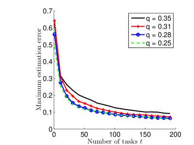
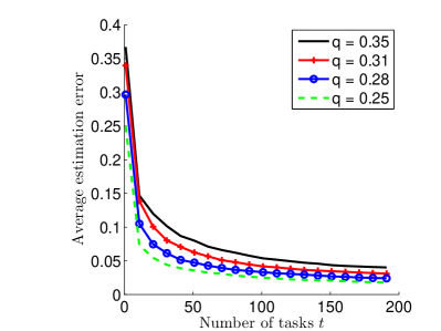
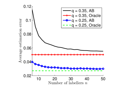
Figure 2 shows the average estimation error of our algorithm for $t=50$ tasks as a function of the number of labellers $n$. We compare our algorithm with an oracle which knows the values of the truth $G(1),\dots,G(t)$ (note that this is different from the oracle used to define the regret, which knows the parameter $p$ and must guess the truth $G(1),\dots,G(t)$). This estimator (which is optimal) simply estimates $p_{i}$ by the empirical probability that labeller $i$ disagrees with the truth. Interestingly, when $n$ increases, the error of our algorithm approaches that of the oracle, showing that our algorithm is nearly optimal.

Figure 2: Average estimation error $\frac{1}{n}||\hat{p}(t)-p||_{1}$ with respect to the number of labellers $n$.

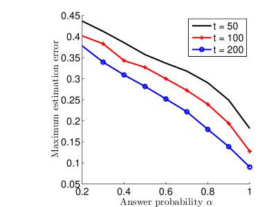
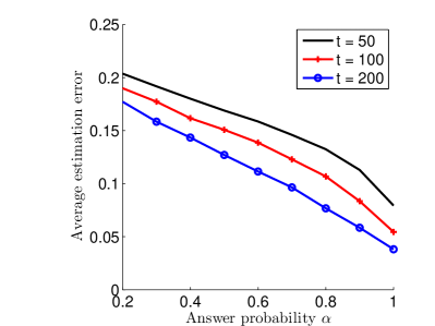
On Figure 3 we present the impact of the answer probability $\alpha$ on the estimation error, for $n=10$ labellers. As expected, the estimation error decreases with $\alpha$. The dependency is approximately linear, which suggests that our upper bound on the estimation error given in Corollary 1, which is inversely proportional to $\alpha^{2}$, can be improved.

(a) Maximum estimation error $||\hat{p}(t)-p||_{\infty}$

(b) Average estimation error $\frac{1}{n}||\hat{p}(t)-p||_{1}$

Figure 3: Estimation error with respect to the anwser probability $\alpha$.

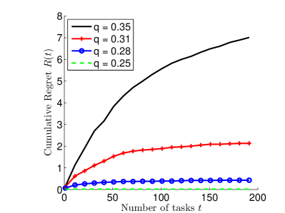
On Figure 4 we present the cumulative regret $R(t)$ with respect to the number of tasks $t$, for $n=10$ labellers and different values of the average error probability $q$. As for the estimation error, the cumulative regret increases with $q$, so that the problem becomes harder as $q$ approaches $1\over 2$, as expected. We know from Theorem 2 that this cumulative regret is finite, for any $q$ that satisfies Assumption 1 (here, $q<0.4$). We observe that this regret is suprisingly low: for $q=0.25$, the cumulative regret is close to 0, meaning that there is practically no difference with the oracle, which knows perfectly the parameter $p$; for $q=0.31$, our algorithm makes less than $2$ prediction errors on average compared to the oracle.

Figure 4: Cumulative regret $R(t)$ with respect to the number of tasks $t$.

6.2 Non-stationary environment

We now turn to non-stationary environments. We assume that the error probability of each labeller evolves as a sinusoid between $0$ and ${1\over 2}$ with some common frequency $\omega$, namely $p_{i}(t)={1\over 4}(1+\sin(\omega t+\varphi_{i}))$. The phases are regularly spaced over $[0,2\pi]$, i.e., $\varphi_{i}=2\pi(i/n)$ for all $i=1,\ldots,n$.

Figure 5: Estimate of $p_{1}(t)$ with respect to the number of tasks $t$, non-stationary environment.

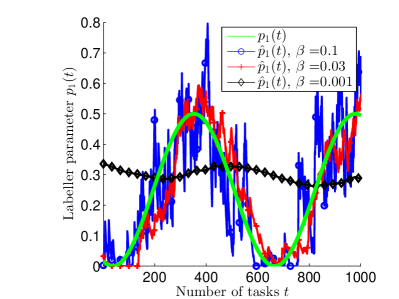
Figure 5 shows the true parameter $p_{1}(t)$ of labeller 1 and the estimated value $\hat{p}_{1}(t)$ on a sample path for $n=10$ labellers, $\omega=10^{-2}$ and various values of the averaging parameter $\beta$. One clearly sees the bias-variance trade-off underlying the choice of $\beta$: choosing a small $\beta$ yields small fluctuations but poor tracking performance, while $\beta$ close to $1$ leads to large fluctuations centered around the correct value. Furthermore, the natural intuition that $p_{1}(t)$ is harder to estimate when it is close to $1\over 2$ is apparent. Finally, for $\beta$ properly chosen (here $\beta=0.03$), our algorithm effectively tracks the evolving latent parameter $p_{1}(t)$.

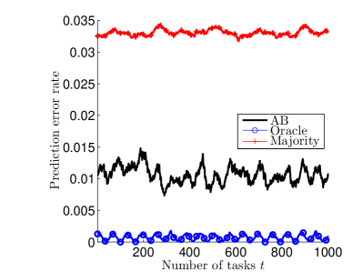
Figure 6 shows the prediction error rate of our algorithm, for $\beta=0.03$, compared to that of majority vote and to that of an oracle that known $p(t)$ exactly for all tasks $t$.

Figure 6: Prediction error rate with respect to the number of tasks $t$, non-stationary environment.

6.3 Real datasets

Finally, we test the performance of our algorithm on real, publicly available datasets (see [21, 23] and references therein), whose main characteristics are summarized in Table 1. When the data set has more than two possible labels (which is the case of the “Dog” and the “Web” datasets), say in the set $\{1,\ldots,L\}$, we merge all labels $\ell\leq L/2$ into label $+1$ and all labels $\ell>L/2$ into label $-1$.

Dataset	# Tasks	# Workers	# Labels
Bird	108	39	4,212
Dog	807	109	8,070
Duchenne	160	64	1,311
Rte	800	164	8,000
Temp	462	76	4,620
Web	2,665	177	15,567

Table 1: Summary of the considered datasets.

Each dataset contains the ground-truth of each task, which allows one to assess the prediction error rate of any algorithm. The results are reported in Table 2 for the following algorithms:

• Majority Vote (MV),

• a standard Expectation Maximization (EM) algorithm known as the DS estimator [4],

• our Agreement-Based (AB) algorithm.

Except for the “Temp” dataset, our algorithm yields some improvement compared to MV, like EM, and a significant performance gain for the “Web” data set, for which more samples are available. The performance of AB and EM are similar for all datasets except for “Bird”, where the number of tasks is limited; this is remarkable given the much lower computational cost of AB, which is linear in the number of samples.

Dataset	MV	EM	AB
Bird	0.24	0.10	0.23
Dog	0.00	0.00	0.00
Duchenne	0.28	0.28	0.26
Rte	0.10	0.07	0.08
Temp	0.06	0.06	0.07
Web	0.14	0.06	0.06

Table 2: Prediction error rates of different algorithms on real datasets.

7 Conclusion

We have proposed a streaming algorithm for performing crowdsourced data classification. The main feature of this algorithm is to adopt a “direct approach” by inverting the relationship between the agreement rates $a$ between various labellers and the latent parameter $p$. This Agreement-Based (AB) algorithm is not a spectral algorithm and does not require to store the task-labeller matrix. Apart from a simple line search, AB does not involve an iterative scheme such as EM or BP.

We have provided performance guarantees for our algorithm in terms of estimation errors. Using this key result, we have shown that our algorithm is optimal in terms of both time complexity (up to logarithmic factors) and regret (compared to the optimal decision). Specifically, we have proved that the cumulative regret is finite, independently of the number of tasks; as a comparison, the cumulative regret of a basic algorithm based on majority vote increases linearly with the number of tasks. We have assessed the performance of AB on both synthetic and real-world data; for the latter, we have seen that AB generally behaves like EM, for a much lower time complexity.

We foresee two directions for future work: on the theoretical side, we want to investigate the extension of AB to more intricate models featuring non-binary labels and where the error probability of labellers depends on the considered task. We would also like to extend our analysis to the sparse regime considered in [9], where the number of answers on a given task does not grow with $n$, so that $\alpha$ is proportional to $1/n$. On the practical side, since AB is designed to work with large data sets provided in real-time as a stream, we hope to be able to experiment its performance on a real-world system.

Appendix A Proof of Theorem 1

We denote by $||\cdot||_{1}$ and $||\cdot||_{\infty}$ the $\ell_{1}$ norm and the $\ell_{\infty}$ norm in $\mathbb{R}^{n}$, respectively.

A.1 Outline

The proof consists of three steps:

1. Concentration of ${\hat{a}}(t)$. Using Hoeffding’s inequality, we prove a concentration inequality on $\hat{a}(t)$.

2. Fixed-point uniqueness. From the concentration of ${\hat{a}}(t)$, we deduce that $v({\hat{a}}(t))$ concentrates around $v(a)$, so that the fixed-point equation $v=f(\hat{a}(t),v)$ has a unique solution with high probability.

3. Smooth dependency between ${\hat{a}}(t)$ and ${\hat{p}}(t)$. When a unique fixed point exists, the mapping ${\hat{a}}(t)\mapsto{\hat{p}}(t)$ depends smoothly on each component of ${\hat{a}}(t)$, which implies the concentration of $\hat{p}(t)$.

A.2 Intermediate results

Recall that (4) is a necessary and sufficient condition for the existence and uniqueness of a solution to the fixed-point equation $v=f(u,v)$. Proposition 4 provides a simpler, sufficient condition. For any $u\in[0,1]^{n}$, let

$$v_{1}(u)=\frac{2}{n}\sum_{i=1}^{n}(2{u}_{i}-1).$$

Proposition 4

If $v_{1}(u)\geq v_{0}(u)$ then there is a unique solution to the fixed-point equation $v=f(u,v)$.

Proof. By the Cauchy-Schwartz inequality,

$$\sum_{i=1}^{n}\sqrt{\delta_{i}(u,v)}\leq\sqrt{n\sum_{i=1}^{n}\delta_{i}(u,v)},$$

so that for all $v>v_{0}(u)$,

$$f(u,v) \leq\frac{n}{(n-2)^{2}}\sum_{i=1}^{n}\delta_{i}(u,v),$$

$$=\frac{1}{(n-2)^{2}}\left({n^{2}}v-\frac{4(n-1)}{n}\sum_{i=1}^{n}(2u_{i}-1)\right),$$

$$=\frac{n^{2}v-2v_{1}(u)(n-1)}{(n-2)^{2}}.$$

In particular,

$$f(u,v)-v\leq 2\frac{n-1}{(n-2)^{2}}(v-v_{1}(u)).$$

If $v_{1}(u)\geq v_{0}(u)$, then $f(u,v_{0}(u))\leq v_{0}(u)$ and there is a unique solution to the fixed-point equation $v=f(u,v)$. $\Box$

Proposition 5 will be used to prove that the fixed-point equation $v=f(u,v)$ has a unique solution for any $u$ in some neighborhood of $a$.

Proposition 5

We have $v_{1}(a)-v_{0}(a)>v(a)$.

Proof. By the definition of $a$,

$$(n-1)\sum_{i=1}^{n}a_{i} =\sum_{i\neq j}(p_{i}p_{j}+(1-p_{i})(1-p_{j}))$$

$$=\left(\sum_{i=1}^{n}p_{i}\right)^{2}+\left(n-\sum_{i=1}^{n}p_{i}\right)^{2}-\sum_{i=1}^{n}(p_{i}^{2}+(1-p_{i})^{2}).$$

Using the fact that $p_{i}^{2}+(1-p_{i})^{2}\leq\frac{1}{2}$ for all $p_{i}\in[0,1]$ and $\sum_{i=1}^{n}p_{i}=nq$, we obtain the lower bound:

$$(n-1)\sum_{i=1}^{n}a_{i}\geq\frac{n}{2}(n(1-2q)^{2}+n-1).$$

In particular,

$$v_{1}(a)=\frac{2}{n}\sum_{i=1}^{n}(2a_{i}-1)\geq\frac{2n}{n-1}(1-2q)^{2}\geq 2v(a).$$

The result follows from the fact that $v_{0}(a)<v(a)$ (see Proposition 3). $\Box$

Let $\mathcal{U}\subset[0,1]^{n}$ be the set of vectors $u$ for which there is a unique solution $v(u)$ to the fixed-point equation $v=f(u,v)$. The following result shows the Lipschitz continuity of the function $u\mapsto v(u)$ on $\mathcal{U}$.

Proposition 6

For all $u,u^{\prime}$ in $\mathcal{U}$,

$$|v(u)-v(u^{\prime})|\leq\frac{8}{n}||u-u^{\prime}||_{1}.$$

Proof. By definition we have $v(u)=f(u,v(u))$ for any $u\in\mathcal{U}$. Since $\frac{\partial f}{\partial v}>1$ (see Proposition 2), by the implicit function theorem, $u\mapsto v(u)$ is differentiable in the interior of $\mathcal{U}$ and

$$\forall i=1,\ldots,n,\quad\frac{\partial v}{\partial{u}_{i}}=\frac{\frac{\partial f}{\partial{u}_{i}}}{1-\frac{\partial f}{\partial v}}.$$

Observing that $\delta_{i}(u,v)$ is positive in the interior of $\mathcal{U}$, we calculate the derivatives of $f$, dropping the arguments $(u,v)$ for convenience:

$$\frac{\partial f}{\partial v} =\frac{1}{(n-2)^{2}}\left(\sum_{i=1}^{n}\sqrt{\delta_{i}}\right)\left(\sum_{i=1}^{n}1/\sqrt{\delta_{i}}\right),$$

$$\frac{\partial f}{\partial{u}_{i}} =-\frac{8(n-1)}{n^{2}(n-2)^{2}}\left(\sum_{j=1}^{n}\sqrt{\delta_{j}/\delta_{i}}\right).$$

Now for all $i=1,\ldots,n$,

$$\frac{\partial f}{\partial v} =\frac{1}{(n-2)^{2}}\left[\left(\sum_{j=1}^{n}\sqrt{\delta_{j}}\right)\left(\sum_{j\neq i}1/\sqrt{\delta_{j}}\right)+\sum_{j=1}^{n}\sqrt{\delta_{j}/\delta_{i}}\right],$$

$$\geq\frac{1}{(n-2)^{2}}\left[\left(\sum_{j\neq i}\sqrt{\delta_{j}}\right)\left(\sum_{j\neq i}1/\sqrt{\delta_{j}}\right)+\sum_{j=1}^{n}\sqrt{\delta_{j}/\delta_{i}}\right],$$

$$\geq\frac{1}{(n-2)^{2}}\left[(n-1)^{2}+\sum_{j=1}^{n}\sqrt{\delta_{j}/\delta_{i}}\right],$$

$$\geq 1+\frac{1}{(n-2)^{2}}\sum_{j=1}^{n}\sqrt{\delta_{j}/\delta_{i}},$$

where we applied Fact 1 to get the second inequality. Thus

$$\frac{\partial f}{\partial v}-1\geq\frac{n^{2}}{8(n-1)}\left|\frac{\partial f}{\partial{u}_{i}}\right|,$$

and

$$\left|\frac{\partial v}{\partial{u}_{i}}\right|\leq\frac{8(n-1)}{n^{2}}\leq\frac{8}{n}.$$

Applying the fundamental theorem of calculus yields the result. $\Box$

A.3 Proof

The proof of Theorem 1 relies on the following two lemmas, giving concentration inequalities on $\hat{a}(t)$ and $\hat{p}(t)$, respectively.

Lemma 1

For any $\epsilon>0$, we have

$$\mathbb{P}(||{\hat{a}}(t)-a||_{\infty}\geq\epsilon) \leq 2n\exp\left(-{2\epsilon^{2}\alpha^{4}t}\right).$$

Proof. In view of (6), for all $i=1,\ldots,n$, ${\hat{a}}_{i}(t)$ is the sum of $t$ independent, positive random variables bounded by $1/(t\alpha^{2})$; in view of (2), we have $\mathbb{E}[{\hat{a}}_{i}(t)]=a_{i}$. By Hoeffding’s inequality,

$$\mathbb{P}(|{\hat{a}}_{i}(t)-a_{i}|\geq\epsilon)\leq 2\exp\left(-{2\epsilon^{2}\alpha^{4}t}\right).$$

The result follows from the union bound. $\Box$

Lemma 2

Let $\epsilon\in(0,\frac{\gamma}{80}]$. If $||{\hat{a}}(t)-a||_{\infty}\leq\epsilon$ then

$$||{\hat{p}}(t)-p||_{\infty}\leq\frac{4}{\gamma^{3/2}}\epsilon.$$

Proof. Assume that $||{\hat{a}}(t)-a||_{\infty}\leq\epsilon$ for some $\epsilon\in(0,\frac{\gamma}{32}]$. Then

$$|v_{0}({\hat{a}}(t))-v_{0}(a)| \leq\frac{8(n-1)}{n^{2}}||{\hat{a}}(t)-a||_{\infty}\leq 8\epsilon$$

and

$$|v_{1}({\hat{a}}(t))-v_{1}(a)|\leq\frac{4}{n}||{\hat{a}}(t)-a||_{1}\leq 4\epsilon.$$

Since $v_{1}(a)-v_{0}(a)>v(a)$ (see Proposition 5) and $v(a)\geq v(a)-v_{0}(a)=\gamma$, we deduce that

$$v_{1}(\hat{a}(t))-v_{0}(\hat{a}(t))>\gamma-{12\epsilon}>0.$$

By Proposition 4, the fixed-point equation $v=f(\hat{a}(t),v)$ has a unique solution. By Proposition 6,

$$|{v}(\hat{a}(t))-v(a)|\leq\frac{8}{n}||{\hat{a}}(t)-a||_{1}\leq{8\epsilon}.$$ (9)

Now for all $i=1,\ldots,n$,

$$|\hat{p}_{i}(t)-p_{i}| =|g_{i}(\hat{a}(t),v({\hat{a}}(t)))-g_{i}(a,v(a))|,$$

$$\leq|g_{i}(\hat{a}(t),v(\hat{a}(t)))-g_{i}(a,v({\hat{a}}(t)))|+|g_{i}(a,v({\hat{a}}(t)))-g_{i}(a,v(a))|.$$

We have

$$\left|\frac{\partial g_{i}}{\partial u_{i}}(u,v)\right|=\frac{n-1}{n\sqrt{\delta_{i}(u,v)}}\leq\frac{1}{\sqrt{\delta_{i}(u,v)}}$$

and

$$\left|\frac{\partial g_{i}}{\partial v}(u,v)\right| =\frac{n}{8}\left|\frac{1}{\sqrt{\delta_{i}(u,v)}}-\frac{1}{\sqrt{v}}\right|\leq\frac{n}{16}\frac{|\delta_{i}(u,v)-v|}{\delta_{i}(u,v)^{3/2}}.$$

Since $\delta_{i}(u,v)\geq v-v_{0}(u)$, we have $\delta_{i}(a,v(a))\geq\gamma$ and for any $u$ in the rectangular box formed by $a$ and $\hat{a}(t)$,

$$\delta_{i}(u,v(\hat{a}(t)))\geq v(\hat{a}(t))-v_{0}(u)\geq\gamma-16\epsilon\geq\frac{4}{5}\gamma.$$

Moreover, $|\delta_{i}(a,v)-v|\leq 4/n$ for any $v$ because $a_{i}\leq 1$ for all $i=1,\ldots,n$, and

$$\delta_{i}(a,v)\geq v-v_{0}(a)\geq\gamma-8\epsilon\geq\frac{9\gamma}{10},$$

for any $v$ between $v(a)$ and $v(\hat{a}(t))$. The fundamental theorem of calculus then gives:

$$|g_{i}(\hat{a}(t),v(\hat{a}(t)))-g_{i}(a,v({\hat{a}}(t)))|\leq\frac{1}{\sqrt{4\gamma/5}}|{\hat{a}}_{i}(t)-a_{i}|$$

and

$$|g_{i}(a,v({\hat{a}}(t)))-g_{i}(a,v(a))|\leq\frac{1}{4(9\gamma/10)^{3/2}}{|{v}(\hat{a}(t))-v(a)|}.$$

We deduce

$$|\hat{p}_{i}(t)-p_{i}|\leq{\sqrt{\frac{5}{4\gamma}}}|{\hat{a}}_{i}(t)-a_{i}|+\frac{1}{4}{\left(\frac{10}{9\gamma}\right)^{3/2}}{|{v}(\hat{a}(t))-v(a)|}.$$

The result then follows from (9), on observing that $\gamma\leq 1$ and $\sqrt{5}/2+2(10/9)^{3/2}\leq 4$. $\Box$

To conclude the proof of Theorem 1, we apply Lemmas 1 and 2 to obtain

$$\mathbb{P}\left(||{\hat{p}}(t)-p||_{\infty}\geq\frac{4}{\gamma^{3/2}}\epsilon\right) \leq\mathbb{P}(||{\hat{a}}(t)-a||_{\infty}\geq\epsilon)\leq 2n\exp\left(-{2\epsilon^{2}\alpha^{4}t}\right),$$

for any $\epsilon\in(0,\frac{\gamma}{80}]$. Taking $\varepsilon=\frac{4}{\gamma^{3/2}}\epsilon$ yields the result, on noting that $\varepsilon\leq\frac{1}{20}$ and $\gamma\leq 1$ imply $\epsilon\leq\frac{\gamma}{80}$.

Appendix B Proof of Theorem 2

We control the regret based on the fact that the oracle and our algorithm output different answers at time $t$ only if $W(t)\equiv\frac{1}{n}\sum_{i=1}^{n}w_{i}X_{i}(t)$ and $\frac{1}{n}\sum_{i=1}^{n}{\hat{w}}_{i}(t)X_{i}(t)$ have different signs.

We first consider the critical case where $W(t)=0$. Let $x\in\{-1,0,1\}$ be such that $w^{T}x=0$. We have

$$\mathbb{P}(G(t)=1,X(t)=x) =\mathbb{P}(G(t)=-1,X(t)=x)={1\over 2}\mathbb{P}(X(t)=x).$$ (10)

The oracle outputs $G(t)$ with probability ${1\over 2}$ so that:

$$\mathbb{P}(G^{\star}(t)\neq G(t),X(t)=x) ={1\over 2}\mathbb{P}(G(t)=-1,X(t)=x)+{1\over 2}\mathbb{P}(G(t)=1,X(t)=x)$$

$$={1\over 2}\mathbb{P}(X(t)=x)$$

Now by the independence of $\hat{w}(t-1)$ and $X(t)$,

$$\mathbb{P}(\hat{G}(t)\neq G(t),X(t)=x) =\mathbb{P}(\hat{w}(t-1)^{T}x>0)\times\mathbb{P}(G(t)=-1,X(t)=x)$$

$$+\mathbb{P}(\hat{w}(t-1)^{T}x<0)\times\mathbb{P}(G(t)=1,X(t)=x)$$

$$+\mathbb{P}(\hat{w}(t-1)^{T}x=0)\times{1\over 2}\mathbb{P}(G(t)=1,X(t)=x)$$

$$+\mathbb{P}(\hat{w}(t-1)^{T}x=0)\times{1\over 2}\mathbb{P}(G(t)=-1,X(t)=x).$$

In view of (10),

$$\mathbb{P}(\hat{G}(t)\neq G(t),X(t)=x)={1\over 2}\mathbb{P}(X(t)=x).$$

Summing over $x$ such that $w^{T}x=0$, we get

$$\mathbb{P}(\hat{G}(t)\neq G(t),W(t)=0)=\mathbb{P}(G^{\star}(t)\neq G(t),W(t)=0)$$

and thus

$$\mathbb{P}(\hat{G}(t)\neq G(t))-\mathbb{P}(G^{\star}(t)\neq G(t))=\mathbb{P}(\hat{G}(t)\neq G(t),W(t)\neq 0)-\mathbb{P}(G^{\star}(t)\neq G(t),W(t)\neq 0).$$

Now if $W(t)\neq 0$, the oracle and our algorithm will output different answers only if

$$\frac{1}{n}\sum_{i=1}^{n}|{\hat{w}}_{i}(t)-w_{i}|\geq|W(t)|.$$

Thus we need to bound the mean estimation error of $w$. Assume $||{\hat{p}}(t)-p||_{\infty}\leq\frac{\eta}{2}$ and let $\epsilon_{i}(t)=\frac{1}{\eta}{|{\hat{p}}_{i}(t)-p_{i}|}\leq 1/2$. We have

$$\hat{p}_{i}(t)\geq p_{i}-\eta\epsilon_{i}(t)\geq p_{i}(1-\epsilon_{i}(t)),$$

and

$$1-\hat{p}_{i}(t)\leq 1-p_{i}+\eta\epsilon_{i}(t)\leq(1-p_{i})(1+\epsilon_{i}(t)).$$

We deduce that

$$|{\hat{w}}_{i}(t)-w_{i}|=\left|\log\left(\frac{p_{i}(1-{\hat{p}}_{i}(t))}{{\hat{p}}_{i}(t)(1-p_{i})}\right)\right|\leq\log\left(\frac{1+\epsilon_{i}(t)}{1-\epsilon_{i}(t)}\right)\leq{4\epsilon_{i}(t)},$$

using inequality $\log z\leq z-1$ and the fact that $\epsilon_{i}(t)\leq 1/2$. Summing the above inequality we get

$$\frac{1}{n}\sum_{i=1}^{n}|{\hat{w}}_{i}(t)-w_{i}|\leq\frac{4}{n}\sum_{i=1}^{n}\epsilon_{i}(t)=\frac{4}{n\eta}\sum_{i=1}^{n}|{\hat{p}}_{i}(t)-p_{i}|\leq\frac{4}{\eta}||\hat{p}(t)-p||_{\infty}.$$

Now

$$r(t) =\mathbb{P}(\hat{G}(t)\neq G(t))-\mathbb{P}(G^{\star}(t)\neq G(t)),$$

$$=\mathbb{P}(\hat{G}(t)\neq G(t),W(t)\neq 0)-\mathbb{P}(G^{\star}(t)\neq G(t),W(t)\neq 0),$$

$$\leq\mathbb{P}(\hat{G}(t)\neq G^{\star}(t),W(t)\neq 0),$$

$$\leq\mathbb{P}\left(||\hat{p}(t)-p||_{\infty}\geq\frac{\eta}{2}\min(|W(t)|/2,1),W(t)\neq 0\right),$$

$$\leq\mathbb{P}\left(||\hat{p}(t)-p||_{\infty}\geq\frac{\lambda\eta}{4}\right).$$

The result then follows from Theorem 1.

For the cumulative regret, we use the inequality $\sum_{t\geq 1}e^{-tz}\leq 1/z$, valid for any $z>0$.

Appendix C Proof of theorem 3

Based on the proof for the stationary case, we adopt the following strategy: we first prove that ${\hat{a}}^{\beta}(t)$ concentrates around $a(t)$ by bounding its bias and fluctuations around its expectation. We then argue that, when ${\hat{a}}^{\beta}(t)$ is close to $a(t)$ then ${\hat{p}}(t)$ must be close to $p(t)$.

C.1 Preliminary results

We start by upper bounding the bias of the estimate $\hat{a}^{\beta}(t)$.

Proposition 7

We have $||\mathbb{E}[{\hat{a}}^{\beta}(t)]-a(t)||_{\infty}\leq{2\sigma\over\beta}$.

Proof. We have:

$$\mathbb{E}[{\hat{a}}^{\beta}_{i}(t)]=\beta\sum_{s=1}^{t}(1-\beta)^{t-s}a_{i}(s).$$

Since

$$a_{i}(t)=\frac{1}{n-1}\sum_{j\neq i}(p_{i}(t)p_{j}(t)+(1-p_{i}(t))(1-p_{j}(t))),$$

we get for all $j\neq i$:

$$\left|\frac{\partial a_{i}}{\partial p_{i}}\right| ={1\over n-1}\left|\sum_{j\neq i}(2p_{j}-1)\right|\leq 1,$$

$$\left|\frac{\partial a_{i}}{\partial p_{j}}\right| ={|2p_{j}-1|\over n-1}\leq{1\over n-1}.$$

We deduce that:

$$\forall s,t\geq 1,\quad|a_{i}(s)-a_{i}(t)| \leq 2||p(s)-p(t)||_{\infty}\leq 2\sigma|s-t|.$$

Hence:

$$||\mathbb{E}[{\hat{a}}^{\beta}(t)]-a(t)||_{\infty} \leq\beta\sum_{s=1}^{t}(1-\beta)^{t-s}||a(s)-a(t)||_{\infty}$$

$$\leq 2\sigma\sum_{s=1}^{t}\beta(1-\beta)^{t-s}|t-s|$$

$$\leq 2\sigma{1-\beta\over\beta}\leq{2\sigma\over\beta}.$$

$\Box$

We next provide a concentration inequality for ${\hat{a}}^{\beta}(t)$.

Proposition 8

For all $\epsilon\geq 0$,

$$\mathbb{P}(||{\hat{a}}^{\beta}(t)-\mathbb{E}[{\hat{a}}^{\beta}(t)]||_{\infty}\geq\epsilon)\leq 2n\exp\left(-\frac{2\epsilon^{2}\alpha^{4}}{\beta}\right).$$

Proof. In view of (8), ${\hat{a}}_{i}^{\beta}(t)$ is a sum of $t$ positive, independent variables, where the $s$-th variable is bounded by $\beta(1-\beta)^{t-s}\alpha^{-2}$. We have the inequality:

$$\sum_{t\geq 1}\beta^{2}(1-\beta)^{2t}=\frac{\beta}{2-\beta}\leq\beta.$$

Hence, from Hoeffding’s inequality,

$$\mathbb{P}(|{\hat{a}}_{i}^{\beta}(t)-\mathbb{E}[{\hat{a}}_{i}^{\beta}(t)]|\geq\epsilon)\leq 2\exp\left(-\frac{2\epsilon^{2}\alpha^{4}}{\beta}\right).$$

The union bound yields the result. $\Box$

C.2 Proof

Let $\epsilon\in(0,{\gamma(t)\over 80}-{2\sigma\over\beta}]$. Assume that

$$||{\hat{a}}^{\beta}(t)-\mathbb{E}[{\hat{a}}^{\beta}(t)]||_{\infty}\leq\epsilon.$$

From Proposition 7, this implies

$$||{\hat{a}}^{\beta}(t)-a(t)||_{\infty} \leq||{\hat{a}}^{\beta}(t)-\mathbb{E}[{\hat{a}}^{\beta}(t)]||_{\infty}+||\mathbb{E}[{\hat{a}}^{\beta}(t)]-a(t)||_{\infty},$$

$$\leq\epsilon+{2\sigma\over\beta},$$

$$\leq{\gamma(t)\over 80}.$$

Applying Lemma 2 yields

$$||{\hat{p}}(t)-p(t)||_{\infty}\leq\frac{4}{\gamma^{3\over 2}(t)}\left(\epsilon+{2\sigma\over\beta}\right).$$

Applying Proposition 8 we get the announced result:

$$\mathbb{P}\Big{(}||{\hat{p}}(t)-p(t)||_{\infty}\geq\frac{4}{\gamma^{3/2}(t)}(\epsilon+\frac{2\sigma}{\beta})\Big{)} \leq\mathbb{P}(||{\hat{a}}^{\beta}(t)-\mathbb{E}[{\hat{a}}^{\beta}(t)]||_{\infty}\leq\epsilon),$$

$$\leq 2n\exp\left(-\frac{2\epsilon^{2}\alpha^{4}}{\beta}\right).$$

References

- [1] P. S. Albert and L. E. Dodd. A cautionary note on the robustness of latent class models for estimating diagnostic error without a gold standard. Biometrics, 60(2):427–435, 2004.
- [2] X. Chen, P. N. Bennett, K. Collins-Thompson, and E. Horvitz. Pairwise ranking aggregation in a crowdsourced setting. In Proceedings of the sixth ACM international conference on Web search and data mining, pages 193–202. ACM, 2013.
- [3] N. Dalvi, A. Dasgupta, R. Kumar, and V. Rastogi. Aggregating crowdsourced binary ratings. In Proceedings of the 22nd international conference on World Wide Web, pages 285–294. International World Wide Web Conferences Steering Committee, 2013.
- [4] A. P. Dawid and A. M. Skene. Maximum likelihood estimation of observer error-rates using the EM algorithm. Journal of the Royal Statistical Society. Series C (Applied Statistics), 28(1):pp. 20–28, 1979.
- [5] A. Ghosh, S. Kale, and R. P. McAfee. Who moderates the moderators?: crowdsourcing abuse detection in user-generated content. In Proceedings 12th ACM Conference on Electronic Commerce (EC-2011), San Jose, CA, USA, June 5-9, 2011, pages 167–176, 2011.
- [6] C.-J. Ho, S. Jabbari, and J. W. Vaughan. Adaptive task assignment for crowdsourced classification. In Proceedings of the 30th International Conference on Machine Learning (ICML-13), pages 534–542, 2013.
- [7] C.-J. Ho and J. W. Vaughan. Online task assignment in crowdsourcing markets. In AAAI, volume 12, pages 45–51, 2012.
- [8] S. L. Hui and S. D. Walter. Estimating the error rates of diagnostic tests. Biometrics, pages 167–171, 1980.
- [9] D. R. Karger, S. Oh, and D. Shah. Iterative learning for reliable crowdsourcing systems. In Advances in Neural Information Processing Systems 24, pages 1953–1961, 2011.
- [10] D. R. Karger, S. Oh, and D. Shah. Efficient crowdsourcing for multi-class labeling. ACM SIGMETRICS Performance Evaluation Review, 41(1):81–92, 2013.
- [11] D. R. Karger, S. Oh, and D. Shah. Budget-optimal task allocation for reliable crowdsourcing systems. Operations Research, 62(1):1–24, 2014.
- [12] Q. Liu, J. Peng, and A. T. Ihler. Variational inference for crowdsourcing. In F. Pereira, C. Burges, L. Bottou, and K. Weinberger, editors, Advances in Neural Information Processing Systems 25, pages 692–700, 2012.
- [13] Y. Liu and M. Liu. An online learning approach to improving the quality of crowd-sourcing. In Proc. of ACM SIGMETRICS, 2015.
- [14] S. Nitzan and J. Paroush. Optimal decision rules in uncertain dichotomous choice situations. International Economic Review, pages 289–297, 1982.
- [15] F. Parisi, F. Strino, B. Nadler, and Y. Kluger. Ranking and combining multiple predictors without labeled data. Proceedings of the National Academy of Sciences, 111(4):1253–1258, 2014.
- [16] V. C. Raykar, S. Yu, L. H. Zhao, G. H. Valadez, C. Florin, L. Bogoni, and L. Moy. Learning from crowds. The Journal of Machine Learning Research, 11:1297–1322, 2010.
- [17] L. Shapley and B. Grofman. Optimizing group judgmental accuracy in the presence of interdependencies. Public Choice, 43(3):329–343, 1984.
- [18] P. Smyth, U. Fayyad, M. Burl, P. Perona, and P. Baldi. Inferring ground truth from subjective labelling of venus images. Advances in Neural Information Processing Systems, pages 1085–1092, 1995.
- [19] D. Wang, T. Abdelzaher, L. Kaplan, and C. C. Aggarwal. Recursive fact-finding: A streaming approach to truth estimation in crowdsourcing applications. In Distributed Computing Systems (ICDCS), 2013 IEEE 33rd International Conference on, pages 530–539. IEEE, 2013.
- [20] P. Welinder and P. Perona. Online crowdsourcing: rating annotators and obtaining cost-effective labels. In Computer Vision and Pattern Recognition Workshops (CVPRW), 2010 IEEE Computer Society Conference on, pages 25–32. IEEE, 2010.
- [21] J. Whitehill, T.-f. Wu, J. Bergsma, J. R. Movellan, and P. L. Ruvolo. Whose vote should count more: Optimal integration of labels from labelers of unknown expertise. In Advances in neural information processing systems, pages 2035–2043, 2009.
- [22] Y. Zhang, X. Chen, D. Zhou, and M. I. Jordan. Spectral methods meet EM: A provably optimal algorithm for crowdsourcing. In Advances in Neural Information Processing Systems 27, pages 1260–1268, 2014.
- [23] D. Zhou, Q. Liu, J. C. Platt, C. Meek, and N. B. Shah. Regularized minimax conditional entropy for crowdsourcing. arXiv preprint arXiv:1503.07240, 2015.