Mathematical control theory, the immune system, and cancer
Abstract
Simple ideas, endowed from the mathematical theory of control, are used in order to analyze in general grounds the human immune system. The general principles are minimization of the pathogen load and economy of resources. They should constrain the parameters describing the immune system. In the simplest linear model, for example, where the response is proportional to the load, the annihilation rate of pathogens in any tissue should be greater than the pathogen’s average rate of growth. When nonlinearities are added, a reference value for the number of pathogens is set, and a stability condition emerges, which relates strength of regular threats, barrier height and annihilation rate. The stability condition allows a qualitative comparison between tissues. On the other hand, in cancer immunity, the linear model leads to an expression for the lifetime risk, which accounts for both the effects of carcinogens (endogenous or external) and the immune response.
pacs:
87.10.Ed, 87.19.lr, 87.19.xb, 87.19.xjImmunity and control. Human immunity is, as there are practically all physical aspects of life, a control process. Our body senses the number of pathogens in a tissue and a response is generated, which reduces the pathogen load.
The system compresses a variety of sensors, signals and effectors at the cellular level Janeway . In the present paper, I would like to present a different perspective, endowed from the mathematical theory of control Teocontrol . The view allows us to stress some general trends and qualitatively compare the response in different tissues.
The general principles are very simple: first, the pathogen load should be minimized, and second, the used resources should be minimal. These principles should constrain the parameters describing the immune system in any tissue.
Linear model. Let us consider, for example, a very small intensity threat to a given tissue in an adult individual. The resident cells of the immune system will trigger a response to clear the infection. These are, basically, resident cells of the innate system ResidentMacroph . The simplest available model for the response is a linear one:
| (1) |
in which the response is proportional to the threat. is time, is the number of pathogens (in some units), and its rate of growth, typically 1/hour for bacteria rate . A freely evolving group of a few streptococci, for example, would lead in around 40 hours to a colony greater than the number of cells in the lungs.
The coefficient , on the other hand, is the tissue annihilation rate of pathogens which, for consistency, should be greater than in order that small threats do not transform into acute health problems in short terms. This condition requires enough number of resident immune cells in the tissue.
Finally, is the rate of entrance of pathogens into the tissue. The constant will model barrier or mucosal immunity, that is, the flow of pathogens, , is partially trapped and cleared by the barrier or mucosa (or both).
According to Eq. (1), a finite load of pathogens is always annihilated, irrespective of the total number. This unrealistic situation is corrected in nonlinear models, characteristic of self-regulated systems.
Nonlinear model. Ref. PLoS, uses different models in order to describe the time evolution of infections in patients. We shall use a modification of their Model 5 in order to take account of nonlinearities:
| (2) |
The parameter equals 0.6 hours-1. The added nonlinearity limits the increase of to values below , a conventional parameter indicating sepsis. Authors of paper [PLoS, ] use an average value of for the body of 1.5 hours-1, a value satisfying the requirement , mentioned in the previous paragraph. The parameter limits also the immune response for high values of .
The main deficiency of Eq. (2) is the lack of a term modeling recruitment of other immune cells. However, even from this simple model, we can get important properties with the help of the qualitative theory of differential equations DiffEqs .

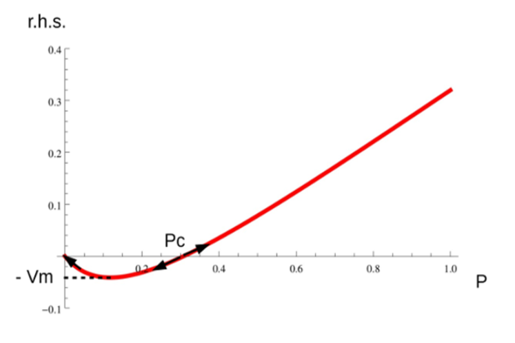
Reference value for the number of pathogens. I draw in Fig. 1 the r.h.s. of Eq. (2) for and =1.5 hours-1, which shows two of the fixed points of the equation: (healthy tissue), and , which is an unstable fixed point dividing healthy from septic conditions. If, in the time evolution according to Eq. (2), reaches values greater than , then the final outcome will be a state with close to . This is the third fixed point of the equation, not seen in the figure.
We can roughly estimate by expanding the r.h.s. of Eq. (2) in series of , retaining linear and quadratic terms, and equating the result to zero, we get:
| (3) |
The last expression comes from neglecting . I will assume that there is a unique for all of the tissues. This sets a reference value for in the whole body. could, probably, be associated to the threshold value for initiating recruitment of additional immune cells.
Stability condition in tissues. The response coefficient , apart from being greater than , depends on the pathogen load the tissue is regularly exposed to. If the flow of pathogens, , is practically constant in certain time intervals, one can get an stability condition by requiring the r.h.s. of Eq. (2) to be lower than zero. This leads to:
| (4) |
is the value at the minimum defined in Fig 1. If the inequality is violated, the r.h.s. of Eq. (2) is always greater than zero and increases towards . The estimation for comes from expanding the r.h.s. in series, in the same way as I did for .
Coefficients and shall combine in each tissue in order to guarantee Eq. (4) to hold, i.e. guarantee immunity against regular threats. Higher threats would require higher barriers (smaller ) and higher annihilation rates (). This is typical of epithelial tissues. In other cases, for example germinal cells in testis, in order to prevent autoimmunity the coefficient is reduced, which is compensated by high barriers. In summary, minimization of leads to the condition (4) for the coefficients and in terms of the regular pathogen flow in the tissue, . Economy of resources implies that the inequality should be near optimal.

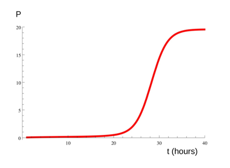
A second consequence of the unstable fixed point. The unstable fixed point not only sets a unique reference value, , but is also the reason for an interesting property of the small- response. When the pathogen load overcomes the stability threshold given by Eq. (4), the fixed point slows down the increase of . The reason is very simple: should traverse the region near , where the r.h.s. of Eq. (2) is near zero, that is, where the annihilation rate of pathogens is close to its rate of growth. This is shown in Fig. 2, where hours-1 and hours-1. The increase of is delayed for more than 20 hours, in spite of the fact that the characteristic time scale of the problem is around one hour. This delay allows recruitment of immune cells from blood circulation.
A qualitative comparison. The following example is a qualitative comparison between two nearby tissues: the small and large intestines. An understanding of the reinforced immunity of the small intestine comes from this analysis.
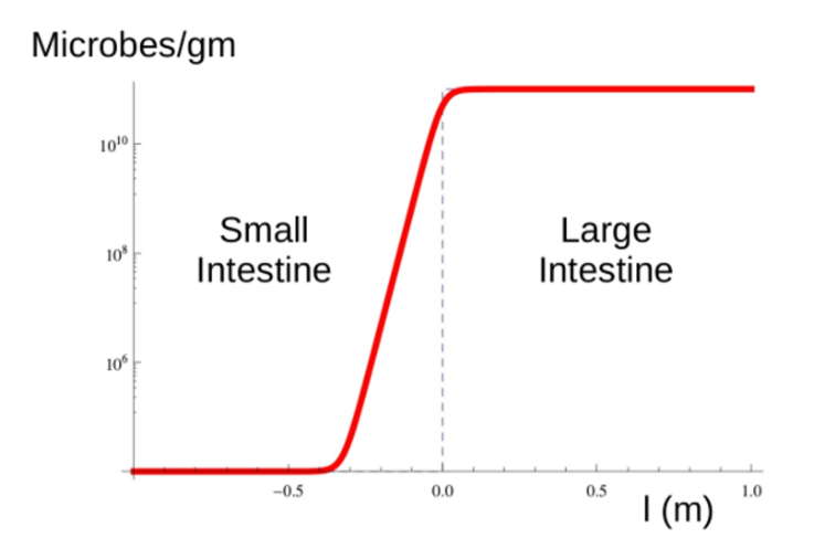
I show in Fig. 3 a schematics of the density of microbes in the contact region. These microbes are mainly commensal bacteria, but it is reasonable to assume that the pathogen loads are proportional to these numbers.
is a coordinate along the gut. The small bowel is located at , and the large intestine at . The mean value of microbes/gm experiences a jump from to as we cross from the ileum to the cecum microbes . Of course, we expect the dependence to be continuous, as schematically represented in Fig. 3.
The parameter values for the large intestine, and , are roughly constant. In the small intestine, however, the parameters shall exhibit a spatial variation. shall decrease and increase as moves towards the distal end of the ileum. Significant variations of the parameters are expected due to the augmented flow of pathogens in many orders of magnitude. This is consistent with the distribution of Paneth cells Paneth , Peyer’s patches Peyer and other structures along the small bowel. Above, the immune protection in the small intestine was said to be “reinforced” in the sense that the coefficients and shall vary in order to increase protection as increases.

Other tissues. The stability condition, Eq. (4), allows also the analysis of tissues in which the flow of pathogens is normal, but is decreased at the expenses of lowering . These are, for example, the brain Blood-Brain and testis Blood-Testis , where a limit to the cellular immune response is needed for a proper functioning of the tissue. Recall that the values for can never be lower than , as mentioned.
In addition, there are also tissues, like the gallbladder, where the microbicide character of bile Bile could be translated into a lower than average and, possibly, a low . Notice that we have generalized the meaning of the “barrier” coefficient, , not limited now to anatomical or mucosal barriers.
In conclusion, I assume that the coefficients and take different values for different tissues. The regular flow the tissue is exposed to, , basically determines the ratio , according to Eq. (4). The tissue’s functioning conditions could dictate additional restrictions. For example, in the brain should be relatively low, thus should be decreased.
Immunity to cancer. Although the detailed dynamics of cancer onset and development is very complex Franck , and partially unknown, one may guess that there should be an inverse correlation between the annihilation rate of pathogens in a tissue, , and the risk of cancer. Indeed, the cellular immune response is not only responsible of eliminating virus infected cells, for example, but also dysfunctional and precancerous cells in the tissue. Thus, a low could be related to a higher than normal cancer risk in that tissue. Conversely, one may obtain information for from the frequency distribution of cancer in the body tissues.
It is reasonable to assume that, for the initial stages of tumors in a tissue, an equation similar to Eq. (1) holds:
| (5) |
where is the (small) number of precancerous cells, is the rate of creation of such cells in the tissue, is their division rate, and - the tissue’s annihilation rate of dysfunctional cells. can be estimated from the division rate of stem cells in that tissue, , assuming that cancer cells originate from stem cells stem . Typically, or even smaller Tomasetti . On the other hand, , as noticed. Thus, .
For , we may use an equation like , where is the number of stem cells, and - a probability parameter modeling the carcinogenic effect of both internal processes (free radicals, for example) or external factors (double strand breaks by ionizing radiation, for example).

Equating to zero the r.h.s. of Eq. (5), we obtain the average number of precancerous cells in the tissue:
| (6) |
In order to become a true tumor, these cells should pass through a few stages Franck , and avoid the adaptive immune system. Nevertheless, it is reasonable to assume that the lifetime risk for cancer in the tissue is proportional to .
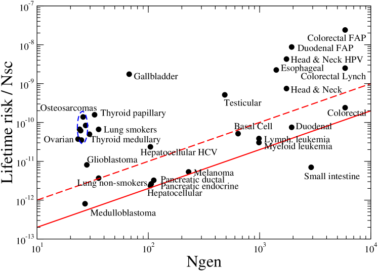
Fig 4 is a re-plot of the results by Tomasetti and Vogelstein Tomasetti (see also Hannun ) showing the dependence of the lifetime risk for cancer in a tissue on the number of stem cells, and the rate of mitotic divisions. The -axis in the figure is the normalized risk, i.e. the risk per stem cell. This normalization allows comparison between tissues with high differences in the number of stem cells. The -axis, on the other hand, counts the number of stem cell generations along lifetime, , a number roughly proportional to the division rate, . The last term accounts for divisions along the clonal expansion phase during tissue formation. The figure shows that, for a single-cell lineage, the larger the higher the normalized risk also.
In Fig. 4, a set of 11 cancers shows a near perfect linear correlation: , where the proportionality coefficient may be roughly written as years, and measures the success rate of precancerous cells: one in ten thousand cells becomes a tumor, for example.
We shall qualify these tissues as “normal”. For all of them, we expect very similar and , although they may exhibit very different barriers (). Indeed, we expect a very low in the colon and skin, but in blood, for example. The only “special” case in this group is the cerebellum, with a high barrier and a normal (instead of a low) . This means a possibility higher than the cerebrum to clear any infection Cerebellum .
External and genetic factors rise the risk (through ) many times, as compared to normal tissues. For example, smoking multiplies the risk for lung cancer by roughly 20 and, in familial adenomatous polyposis patients, the risk for colon cancer is increased by a factor around 100.
There are also tissues like the brain, germ cells, gallbladder, bones and the thyroid where, in addition to genetic or external factors, the relatively high normalized values for the risk lead one suspect unusually low values of . The brain, germ cells and the gallbladder were briefly discussed above. With regard to bones, it is known that immunity relies strongly on defensins Bones , possibly with a relatively low number of resident cells. On the other hand, the thyroid is known to have a close cross-talk with the immune system Thyroid . It’s dysregulation is the cause of immune disorders. One may speculate that a low number of resident cells is needed in order to prevent autoimmunity in the thyroid.
Finally, we have the small intestine with a normalized risk lower than normal, possibly related to a high averaged , a fact consistent with what was discussed above.
The results for the estimated coefficients are summarized in Table 1. Although they are only qualitative results, they allow comparison between tissues, and are a first step towards the understanding of Fig. 4 for the lifetime risks of cancer in different tissues.
| Tissue | Regular pathogen flow () | Barrier height () | Annihilation rate () |
| Small intestine | Very High | High | High |
| Colon | Very High | Very High | Normal |
| Lung | Very High | Very High | Normal |
| Skin | Very High | Very High | Normal |
| Duodenum | High | High | Normal |
| Blood | Normal | Normal | Normal |
| Pancreas | Normal | Normal | Normal |
| Liver | High | High | Normal |
| Cerebellum | Normal | High | Normal |
| Germ cells | Normal | High | Low |
| Brain | Normal | High | Low |
| Gallbladder | Normal | High | Low |
| Bone | Normal | High | Low |
| Thyroid | Normal | High | Low |
| Esophagus | High | High | Normal |
| Head and Neck | Normal | Normal | Normal |
Concluding remarks. In the paper, I show that simple ideas, coming from control theory, lead to interesting results when applied to the human immune system.
In the first step, the linear model described by Eq. (1), it is shown that stability of a tissue against small pathogen threats requires . If this condition is not fulfilled, a small threat would, in a few hours, become a serious health problem.
The linear model is modified, Eq. (2), in order to consider that neither the number of pathogens nor the response can grow without limits. Healthy () and septic () states appear as fixed points of the nonlinear (self-regulated) equation. In the middle of the way, an additional unstable fixed point, , signals the transition from healthy to septic regimes. I postulate that is common to all tissues. At this step, the stability condition is formulated as, Eq. (4):
this inequality relates the regular flow of pathogens in the tissue, , with the coefficients and . We may have, for example, a very high along with a very small and a normal , as in the colon. Or a normal , a small and a small , as in the brain.
I notice that the distribution frequency of cancer in tissues provides indications about the strength of . This statement follows from an estimation of the stationary number of precancerous cells in the tissue, which involves both the probabilities of carcinogenic factors and the strength of the immune response. A low , as it is presumably the situation in the gallbladder, for example, would mean a higher than average number of precancerous cells in the tissue. These cells shall evolve and succeed in avoiding the adaptive system in order to give rise to a cancer.
I hope that the model’s simplicity and the qualitative results following from it will motivate immunologists to quantify in more precise terms the immune response in tissues and in the whole body.
Acknowledgments. The author acknowledges support from the National Program of Basic Sciences in Cuba, and from the Office of External Activities of the International Center for Theoretical Physics (ICTP).
References
- (1) C.A. Janeway, Jr, P. Travers, M. Walport, and M.J. Shlomchik, Immunobiology, New York: Garland Science; 2001.
- (2) A. Bressan and B. Piccoli, Introduction to the Mathematical Theory of Control, AIMS series on applied mathematics, Vol. 2, 2007.
- (3) See, for example, the articles in the review number: Tissue-resident leukocytes, Nat. Immunol. 2013; 14(10).
- (4) H.J. Beckers and J.S. van der Hoeven, Growth rates of Actinomyces viscosus and Streptococcus mutans during early colonization of tooth surfaces in gnotobiotic rats, Infect. Immun.; 35(2): 583–587 (1982).
- (5) M. Mai, Kun Wang, G. Huber, M. Kirby, M.D. Shattuck, Corey S. O’Hern, Outcome Prediction in Mathematical Models of Immune Response to Infection, (2015) PLoS ONE 10(8): e0135861.
- (6) V.V. Nemytskii, V.V. Stepanov, Qualitative theory of differential equations, Princeton University Press, Princeton, 1960.
- (7) A.M. O’Hara and F. Shanahan, The gut flora as a forgotten organ, EMBO Rep. 2006; 7(7): 688–693 (2006).
- (8) H.C. Clevers, C.L. Bevins, Paneth cells: maestros of the small intestinal crypts, Annu. Rev. Physiol. 2013;75:289-311.
- (9) C. Jung, J.P. Hugot, and F. Barreau, Peyer’s Patches: The Immune Sensors of the Intestine, Int. J. Inflam. 2010; 2010: 823710.
- (10) N.M. Van Sorge, Defense at the border: the blood-brain barrier versus bacterial foreigners, Future Microbiol. 7: 383-394 (2012).
- (11) L.R. França, S.A. Auharek, R.A. Hess, J.M. Dufour and B.T. Hinton, Blood-Tissue Barriers: Morphofunctional and Immunological Aspects of the Blood-Testis and Blood-Epididymal Barriers, in Biology and Regulation of Blood-Tissue Barriers, Ed. C. Yan Cheng, Ch. 12, pp. 237-259, Landes Bioscience and Springer, 2012.
- (12) M.E. Merritt and J.R. Donaldson, Effect of bile salts on the DNA and membrane integrity of enteric bacteria, Journal of Medical Microbiology, 58, 1533–1541 (2009).
- (13) S.A. Frank, Dynamics of cancer : incidence, inheritance, and evolution, Princeton University Press, Princeton, New Jersey, 2007.
- (14) T. Reya, S.J. Morrison, M.F. Clarke and I.L. Weissman, Stem cells, cancer, and cancer stem cells, Nature 414, 105–111 (2001).
- (15) C. Tomasetti and B. Vogelstein, Variation in cancer risk among tissues can be explained by the number of stem cell divisions, Science 347, 78-81 (2015); Supplementary materials: www.sciencemag.org/content/347/6217/78/suppl/.
- (16) S. Wu, S. Powers, W. Zhu, and Y.A. Hannun, Substantial contribution of extrinsic risk factors to cancer development, Nature 529, 43-47 (2016).
- (17) T.W. Phares, R.B. Kean, T. Mikheeva, and D. Craig Hooper, Regional Differences in Blood-Brain Barrier Permeability Changes and Inflammation in the Apathogenic Clearance of Virus from the Central Nervous System, J. Immunol., 176: 7666-7675 (2006).
- (18) D. Varoga, C.J. Wruck, M. Tohidnezhad, et. al., Osteoblasts participate in the innate immunity of the bone by producing human beta defensin-3, Histochem. Cell Biol. 2009;131(2):207-18.
- (19) C. Perrotta, C. De Palma, E. Clementi, and D. Cervia, Hormones and immunity in cancer: are thyroid hormones endocrine players in the microglia/glioma cross-talk?, Front. Cell Neurosci. 2015; 9: 236.