Modelling collinear and spatially correlated data

Abstract

In this work we present a statistical approach to distinguish and interpret the complex relationship between several predictors and a response variable at the small area level, in the presence of i) high correlation between the predictors and ii) spatial correlation for the response.

Covariates which are highly correlated create collinearity problems when used in a standard multiple regression model. Many methods have been proposed in the literature to address this issue. A very common approach is to create an index which aggregates all the highly correlated variables of interest. For example, it is well known that there is a relationship between social deprivation measured through the Multiple Deprivation Index (IMD) and air pollution; this index is then used as a confounder in assessing the effect of air pollution on health outcomes (e.g. respiratory hospital admissions or mortality). However it would be more informative to look specifically at each domain of the IMD and at its relationship with air pollution to better understand its role as a confounder in the epidemiological analyses.

In this paper we illustrate how the complex relationships between the domains of IMD and air pollution can be deconstructed and analysed using profile regression, a Bayesian non-parametric model for clustering responses and covariates simultaneously. Moreover, we include an intrinsic spatial conditional autoregressive (ICAR) term to account for the spatial correlation of the response variable.

Keywords: profile regression, Bayesian clustering, spatial modelling, collinearity, index of multiple deprivation, pollution.

1 Introduction

In many statistical applications a common challenge arises when trying to assess meaningful relationships between explanatory variables and outcomes through regression models, due to the potential collinearity of the explanatory variables. This issue is well known in epidemiological or social studies, for instance where questionnaires or surveys collect information on a large number of potential risk factors for particular end points; in this context a simplistic approach consists in examining each variable in turn to avoid the instability in the estimates due to the collinearity, making it impossible to judge the more realistic complex relationship involving several risk factors at the same time. A different approach combines all the relevant variables into summary scores or indexes and assesses the relationship of these with the outcome of interest, which is free from the collinearity issue, but loses information on the single variables included in the summary.

Recently, Dirichlet process mixture models have been used as an alternative to regression models (Dunson et al., 2008; Bigelow and Dunson, 2009). In this paper we focus on the model known as profile regression and proposed by Molitor et al. (2010). Profile regression is a Bayesian non–parametric method which assesses the link between potentially collinear variables and a response through cluster membership. This allows to formally take into account the correlation between the variables without the need to create a summary score, giving more flexibility to the inferential process. Profile regression has been used on several applications in environmental and social epidemiology and the R package PReMiuM (Liverani et al., 2015) makes it readily available to any applied researcher. For instance Molitor et al. (2010) considered the National Survey of Children’s Health and in particular investigated a large number of health and social related variables on mental health of children age 6–17, while Papathomas et al. (2011) focussed on profiles of exposure to environmental carcinogens and lung cancer in the EPIC European cohort. Profile regression has also been used in environmental epidemiology (Pirani et al., 2015), for studying risk functions associated with multi-dimensional exposure profiles (Hastie et al., 2013; Molitor et al., 2014) as well as for looking for gene-gene interactions (Papathomas et al., 2012).

In its present formulation, profile regression has only been used for studies based on cohorts or surveys where information on the predictors/outcomes is available on each individual; in this paper we extend the method to fit small area studies, commonly used in epidemiological surveillance (see for instance Elliott and Wartenberg 2004) or in studies where the interest lies on the spatial variability of an outcome (Barcelo et al., 2009) or on cluster detection (Abellan et al., 2008; Li et al., 2012). In this types of studies information is available at the area level rather than at the individual level and space is used as a proxy for any unmeasured variable; the common assumption is that areas which are close to each other are more similar than those further apart, suggesting that an additional source of correlation, namely spatial correlation needs to be accommodated in the models. We incorporate it in the model through a conditional autoregressive structure (Besag et al., 1991) based on a neighborhood definition, thus assuming that conditional on the neighborhood structure, two areas are independent from each other if they do not share boundaries. We apply the spatial profile regression to the problem of environmental and social inequalities in London, jointly modelling social deprivation and air pollution to highlight the presence of environmental justice.

The paper is structured as follows. In Section 2 we present the motivating example for our methodological development of the spatial profile regression, introducing the context of social and environmental inequalities and how they are related; we also describe the available data. In Section 3 we provide a brief summary of the profile regression and present how to extend it to include spatial correlation. In Section 4 we illustrate how the model works on evaluating the relationship between social deprivation and air pollution. Section 5 presents some discussion points and ideas for future work.

2 Example: social deprivation and air pollution in London

The scientific literature reports mixed evidence on the link between socio-economic status and air pollution. Recent studies indicated that air pollution tends to influence most deprived groups, suggesting that people with lower socio-economic status are more likely to live in a more hazardous and polluted living environment, accidentally or deliberately (Brown, 1995; O’Neill et al., 2003; Blowers and Leroy, 1994; Morello-Frosch et al., 2002). In particular, ecological studies using small areas such as neighbourhoods, census tracts and post codes, report this association, while studies carried out at a lower spatial resolution (e.g. region, country), thus characterised by more aggregate measurements of socio-economic characteristics, showed either non-existent or negative associations (Davidson and Anderton, 2000; Laurent et al., 2007), presumably due to the large within-area variability not taken into account, or even an inverse association, with higher exposures in less deprived groups (Perlin et al., 1995). In the UK several studies reported positive or non-linear correlation between environmental pollution and the deprivation index at both small area level and country level. However the results varied depending on the selection of environmental hazards and scale of analysis (Briggs et al., 2008), calling for some more research on the topic.

Understanding environmental and social inequalities is a key issue as growing health disparities appear between people with socially disadvantaged and privileged social classes, which can translate into increased mortality or morbidity for the low socio-economic groups across a wide range of diseases (Brulle and Pellow, 2006; Benach et al., 2001), including lung cancer (Pope et al., 2011), cardiovascular events (Tonne et al., 2007; Peters et al., 2004), and childhood respiratory diseases (Morgenstern et al., 2007).

In addition, the exposure of air pollution can lead to negative health outcomes acutely or chronically (Chen et al., 2008). Previous studies reported possible mechanisms to explain how environmental exposures result in greater health impact among socially disadvantaged groups, who may have increased susceptibility to the effect of these exposures because of limited access to health care and psychosocial stress; underlying health conditions such as cardiovascular diseases and respiratory diseases that increase susceptibility to the effect of these exposure may also vary between deprived and privileged populations (O’Neill et al., 2003; Morello-Frosch and Jesdale, 2006). These environmental exposure inequalities are increasingly considered as a potential determinant of health disparities (Morello-Frosch and Jesdale, 2006). In addition, it has been suggested that the disparities grow in more deprived areas as health improves faster in high socio-economic groups (Leyland et al., 2007; Higgs et al., 1998).

Although individual determinants (such as smoking) or individual risk responses (such as closing windows to avoid exposure) may frequently contribute to these health inequities, only a fraction of the overall disparities are attributed to individual factors (Lantz et al., 2001). In fact, human health is not only influenced by individual health behaviours but also by contextual and ecological factors (Marmot, 2007). Furthermore, socio-economic status plays a potential role of confounding or effect modification in epidemiological studies investigating the relationship between environmental variables and health outcomes, especially at aggregated level (Blakely and Woodward, 2000; Blakely et al., 2004). The further effect of confounding and effect modification will potentially lead to bias of the results, whose level depends on the relationship between environmental pollutions and socio-economic status. Hence it is extremely important to study this association, which, at the moment still remains uncertain and subjected to the fundamental methodological issue of correlation between variables.

To study this relationship in the present work we consider the following data:

• nitrogen oxides (NO_x), which is generated mainly through combustion, thus is a good proxy for traffic related air pollution. The data were obtained from the environmental research group at Kings College as annual mean for the period 2003-2010 at the Lower Super Output Area geographical level in Greater London (LSOA, 4,767 in Greater London) as part of the TRAFFIC project (http://www.kcl.ac.uk/lsm/research/divisions/aes/research/ERG/research-projects/traffic/index.aspx).

• Index of Multiple Deprivation (IMD), publicly available from the Department for Communities and Local Government (data.gov.uk). It is commonly used at the small area level to synthesize multiple aspects of deprivation. It is originally built at LSOA level and is formed by 38 indicators collapsed into seven domains: Income, Employment, Health, Education, Crime, Access to Services (Housing) and Living Environment. As we want to evaluate the relationship between the domains of the IMD and air pollution (NOx) we have not considered the living environment domain, which includes air quality. IMD is available for 2004, 2007 and 2010 and we have considered the most recent one in this work (correlation between Index at different years ranges from 0.94 and 0.97).

(a) NO_x concentration for 2003-2010

(b) IMD score, 2010

Figure 1: Quintilesof the NO_x concentration (average 2003-2010) and of IMD score (2010) at LSOA level in Greater London.

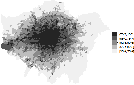
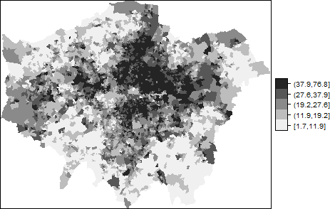
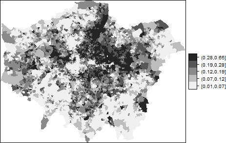
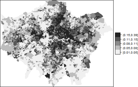
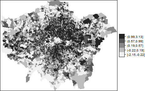
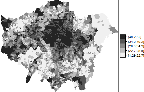
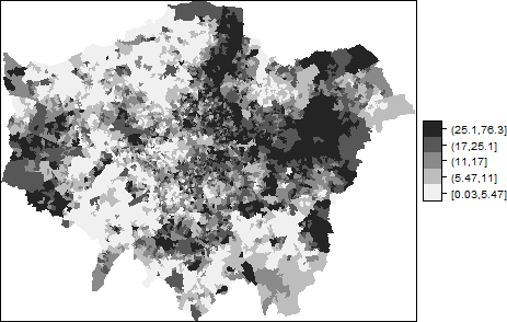
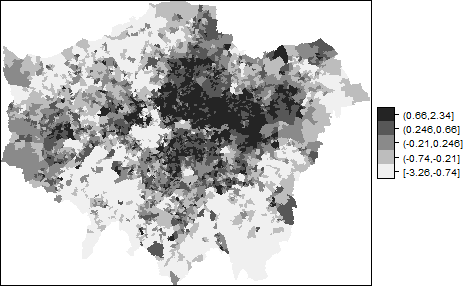
Figure 1 shows the map for NO_x (left) and IMD score (right) and a clear spatial pattern is visible in both: air pollution concentration increases steadily going from outer to inner London, while IMD shows the highest deprived areas in the northeastern part of London and most of the central southern part. However looking at the maps of each of the six domains highlights a different picture (Figure 2): Crime shows the absence of a clear pattern, with scattered areas of high crime (dark grey) next to areas of low crime (light grey); on the other hand income, employment and health/disability are in agreement with the total IMD score, while barriers to housing and services are more pronounced in central London and education shows more deprivation in East London. This suggests how simplistic is the approach that considers the total IMD score and highlights the importance of including all the domains to disclose the relationship between social characteristics and environmental pollution at a small area level.

If we want to investigate the relationship between each domain and air pollution we cannot include all the domains in a regression model due to their collinearity issues: the pairwise Pearson correlation between domains (Table 1) shows high values for income and employment (0.91), income and health (0.77), income and education (0.68), employment and health (0.81) and employment and education (0.64).

Table 1: Correlation between IMD domains. In bold correlation higher than 0.6.

	Income	Employ.	Health	Educ.	Hous.	Crime
Income	1.0	0.91	0.77	0.68	0.48	0.52
Employ.	0.91	1.0	0.81	0.64	0.42	0.53
Health	0.77	0.81	1.0	0.55	0.41	0.59
Educ.	0.68	0.64	0.55	1.0	0.16	0.36
Hous.	0.48	0.42	0.41	0.16	1.0	0.29
Crime	0.52	0.53	0.59	0.37	0.29	1.0

(a) Income

(b) Employment

(c) Crime

(d) Barriers to Housing and Services

(e) Education

(f) Health and Disability

Figure 2: Maps of the six IMD domains considered: quintiles of the scores (note that higher positive values means higher deprivation.

3 Modelling highly correlated covariates with profile regression

To include all the domains into the same statistical model we use the profile regression, a model that non-parametrically links a response vector $\bm{Y}$ to covariate data $\bm{X}$ through cluster membership. It was proposed by Molitor et al. (2010) and it has been implemented in the R package PReMiuM (Liverani et al., 2015).

Profile regression implements a Bayesian clustering model through a Dirichlet process mixture model. The data $\bm{D}=(\bm{Y},\bm{X},\bm{W})$ contain the response $\bm{Y}$, covariate $\bm{X}$ and fixed effects $\bm{W}$ if they are available. The fixed effects are potentially confounding variables. In our running example the response is the nitrogen oxides, the covariates are the selected six domains of IMD and we do not include fixed effects.

For each individual $i$, for $i=1,\ldots,n$, the response is given by $y_{i}$, the covariate vector $\mathbf{x}_{i}$ and the fixed effect vector $\mathbf{w}_{i}$. The data are then jointly modelled as the product of a response model and a covariate model, leading to the following likelihood:

$$f(\mathbf{x}_{i},y_{i}|\bm{\Theta}_{Z_{i}},\bm{\Lambda},W_{i},\psi)=\sum_{c}\psi_{c}f(\mathbf{x}_{i}|z_{i}=c,\phi_{c})f(y_{i}|z_{i}=c,\theta_{c},\bm{\Lambda},\mathbf{w}_{i})$$

where $z_{i}=c$, the allocation variable, indicates that individual $i$ belongs to cluster $c$. The parameters $\bm{\Lambda}=(\bm{\theta},\bm{\phi})$ are cluster specific and represent the contribution of the response and the covariates to the mixture model. There is also the possibility to include additional fixed effects $\mathbf{w}_{i}$ for each individual, which are constrained to only have a global (i.e., non-cluster specific) effect on the response $y_{i}$. The parameters $\psi$ are the mixture weights.

Multicollinearity arises when regression models of the response with respect to highly correlated covariates are implemented, due to identifiability issues. However, as here the response is conditionally independent from the covariates, we do not encounter such issues, but we can explore in depth the potentially complex relationship between response and covariates.

The prior model for the mixture weights is given by the stick-breaking priors (constructive definition of the Dirichlet process), that is,

$$\psi_{c} = V_{c}\prod_{l<c}(1-V_{l})\quad\mbox{for all $c$},$$

$$\psi_{1} = V_{1},$$

$$V_{c} \sim \mbox{Beta}(1,\alpha)\quad\mbox{i.i.d.}$$

The parameter $\alpha$ can be fixed or can have a Gamma$(s_{\alpha},r_{\alpha})$ distribution with $s_{\alpha}$ and $r_{\alpha}$ as shape and rate parameters respectively. Other prior models for the mixture weights are possible, and, for example, the Pitman-Yor construction is also available in the R package PReMiuM.

The covariate model $f(\mathbf{x}_{i}|z_{i}=c,\phi_{c})$ can be defined as continuous or discrete. In the continuous case $\bm{X}$ assumes a mixture of Gaussian distributions. In the discrete case for each individual $i$, $\mathbf{x}_{i}$ is a vector of $J$ locally independent discrete categorical random variables, where the number of categories for covariate $j=1,2,\ldots,J$ is $K_{j}$. Then we can write $\Phi_{c}=(\Phi_{c,1},\Phi_{c,2}\ldots,\Phi_{c,J})$ with $\Phi_{c,j}=(\phi_{c,j,1},\phi_{c,j,2},\ldots,\phi_{c,j,K_{j}})$ and

$$f(\mathbf{x}_{i}|z_{i}=c,\phi_{c})=\prod_{j=1}^{J}\phi_{{Z_{i}},j,X_{i,j}}.$$ (1)

We let $a=(a_{1},a_{2},\ldots,a_{J})$, where for $j=1,2,\ldots,J$, $a_{j}=(a_{j,1},a_{j,2},\ldots,a_{j,K_{j}})$ and $\Phi_{c,j}\sim\mbox{Dirichlet}(a_{j})$. The covariate model can also be defined as a mixture of continuous and discrete covariates.

The response model $f(y_{i}|z_{i}=c,\theta_{c},\bm{\Lambda},\mathbf{w}_{i})$ can be defined as binary, categorical, count (modelled as Binomial or Poisson) or Gaussian. For example, for Gaussian response the mixture model is extended to contain $\theta_{c}$ for each $c$ and the global parameters $\bm{\Lambda}=(\bm{\beta},\sigma^{2}_{Y})$. These parameters allow us to write the response model as:

$$f(y_{i}|z_{i}=c,\theta_{c},\bm{\Lambda},W_{i})=f(y_{i}|z_{i}=c,\theta_{c},\bm{\beta},\sigma^{2}_{Y},W_{i})=\frac{1}{\sqrt{2\pi\sigma^{2}_{Y}}}\exp\left\{-\frac{1}{2\sigma^{2}_{Y}}(Y_{i}-\lambda_{i})^{2}\right\},$$

where $\lambda_{i}=\theta_{Z_{i}}+\bm{\beta}^{\top}W_{i}$ and $\bm{\beta}$ represent the effect of the counfounding variables, the fixed effects, on the response. For each cluster $c$, we adopt a $t$ location-scale distribution on $\theta_{c}$, with hyperparameters $\mu_{\theta}$ and $\sigma_{\theta}$ with 7 degrees of freedom. Similarly, we adopt the same prior for the fixed effect $\beta_{k}$, but with hyperparameters $\mu_{\beta}$ and $\sigma_{\beta}$. We set $\tau_{Y}=1/\sigma_{Y}^{2}$ to Gamma$(s_{\tau_{Y}},r_{\tau_{Y}})$, where $s_{\tau_{Y}}$ and $r_{\tau_{Y}}$ are the shape and rate hyperparameters.

More details on the Markov chain Monte Carlo (MCMC) algorithm for this model are provided in Liverani et al. (2015). When the signal in the data is strong the MCMC results for different runs, with different initial values and chain lengths, give stable results. However, this is not the case when the signal is not strong. Hastie et al. (2015) discuss strategies to identify convergence issues. They recommend starting the MCMC with a large number of clusters as the algorithm can struggle to explore the partition space when starting with a small number of clusters if the signal is not strong. When many clusters are identified it is more challenging to characterise each cluster meaningfully and interpretation of the results can be facilitated by the posterior predictive distrbution. Moreover, they suggest the use of the posterior distribution of predictive profiles for the assessment of convergence instead of the posterior distribution of the parameters. This is because the posterior distribution of the parameters can appear to have converged when the model as a whole has not (often the case for $\bm{\beta}$), or cannot be used for this scope because they are cluster-specific and the number of clusters changes at each iteration (such as $\theta_{c}$).

It is often useful to characterise the partition which is most supported by the data. However, as at each iteration of the sampler individual profiles are assigned to clusters, the MCMC output is very rich. Molitor et al. (2010) developed methods to process this output to make useful and interpretable inference. Several methods for this are available in the R package PReMiuM but we find the most robust method is to process the similarity matrix using partitioning around medoids (PAM), which is available in the R package cluster. First of all, a score matrix is constructed, where each element of the matrix is set equal to 1 if individuals $i$ and $j$ belong to the same cluster and 0 otherwise. Then a similarity matrix $S$ is computed by dividing each element of the score matrix by the number of iterations, so that $S_{ij}$ denotes the probability that individuals i and j are assigned to the same cluster. PAM then assigns individuals to clusters in a way consistent with matrix $S$.

3.1 The Spatial Conditional Autoregressive Model

When clustering data from small area studies, we need to modify the model to account for spatial correlation. In this paper we propose to extend the response model described above to include an intrinsic spatial conditional autoregressive (ICAR) term (Besag et al., 1991) as follows. The likelihood component for the Gaussian response becomes

$$f(y_{i}|z_{i}=c,\theta_{c},\bm{\Lambda},W_{i})=f(y_{i}|z_{i}=c,\theta_{c},\bm{\beta},\sigma^{2}_{Y},u_{i},W_{i})=\frac{1}{\sqrt{2\pi\sigma_{Y}^{2}}}\exp(-\frac{1}{2\sigma_{Y}^{2}}(Y_{i}-\lambda_{i})^{2})$$

where $\lambda_{i}=\theta_{Z_{i}}+W_{i}\bm{\beta}+u_{i}$ and $u=(u_{1},\cdots,u_{n})\sim N(0,\mathbf{\tau P})$ with $\mathbf{P}=\{P_{ij}\}$ a precision matrix such that

$$P_{ij}=\begin{cases}n_{i}&\mbox{if}\;i=j\\ -I\{i\sim j\}&\mbox{if}\;i\neq j\\ \end{cases}$$

where $n_{i}$ is the number of neighbours of subject $i$, $I$ is the indicator function and $i\sim j$ indicates that regions $i$ and $j$ are neighbours. The prior of $\tau$ is given by

$$\tau\sim\mbox{Gamma}(a_{\tau},b_{\tau})$$

such that

$$E(\tau)=\frac{a_{\tau}}{b_{\tau}}\quad and\quad\mbox{Var}(\tau)=\frac{a_{\tau}}{b_{\tau}^{2}}.$$

Details of the sampling strategy for the ICAR parameters are given in Appendix A. We have implemented this model in the R package PReMiuM for Gaussian and Poisson responses.

4 Results

We have fit profile regression to the data using the R package PReMiuM (Liverani et al., 2015). The pollution data are modelled with a Gaussian distribution including a spatial ICAR term. The covariate profiles, given by the selected IMD domains, are modelled with a discrete distribution, as we have transformed each IMD domain into quintiles. We have not included any additional fixed effects. The results were very robust on several MCMC runs using a range of initial values and different chain lengths. We present here the results obtained with 5,000 iterations after a burn in of 5,000 with the following hyperparameter settings.

$$s_{\alpha}=2,\quad\quad r_{\alpha}=1,$$

$$a_{1}=\ldots=a_{6}=1,$$

$$\mu_{\theta}=0,\quad\sigma_{\theta}=2.5,$$

$$\mu_{\beta}=0,\quad\sigma_{\beta}=2.5,$$

$$s_{\tau-Y}=2.5,\quad r_{\tau-Y}=2.5.$$

Figure 3: Geographical representation of the eleven clusters of the areas in Greater London identified by profile regression. The colours reflect the mean of the observed pollution levels, with dark grey identifying the most polluted clusters and light grey the least polluted clusters.

In this section we aim to illustrate how profile regression can help shed light on complex patterns between highly covariates covariates and response. We propose several ways to explore the results.

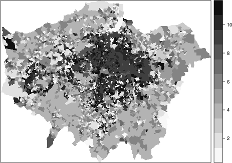
The main output of profile regression are the clusters, given by regions with similar covariate and response characteristics. We have used different types of plots, which highlight specific features, at different level of details. In Figure 3 we represent the clusters geographically. The eleven clusters identified are plotted using colours that reflect their observed pollution levels. As expected, the most central areas have higher pollution levels. In particular we see that areas that belong to clusters with higher observed pollution levels are mostly located in North-East London, where areas with higher levels of deprivation are found. In contrast, the less deprived areas in South-West London are clustered together and have lower mean for the observed pollution levels.

Figure 4: Summary plot of the posterior distribution of the parameters $\Phi_{c}$, for $c=1,\ldots 11$. Each column $j$ in the figure represents $\Phi_{c,j,k}$, for $c=1,\ldots,11$ and $k=0,1,\ldots,4$. Within a column $j$, each row $k$ is a visualisation of the boxplots for $\phi_{c,j,k}$ for each cluster $c$.

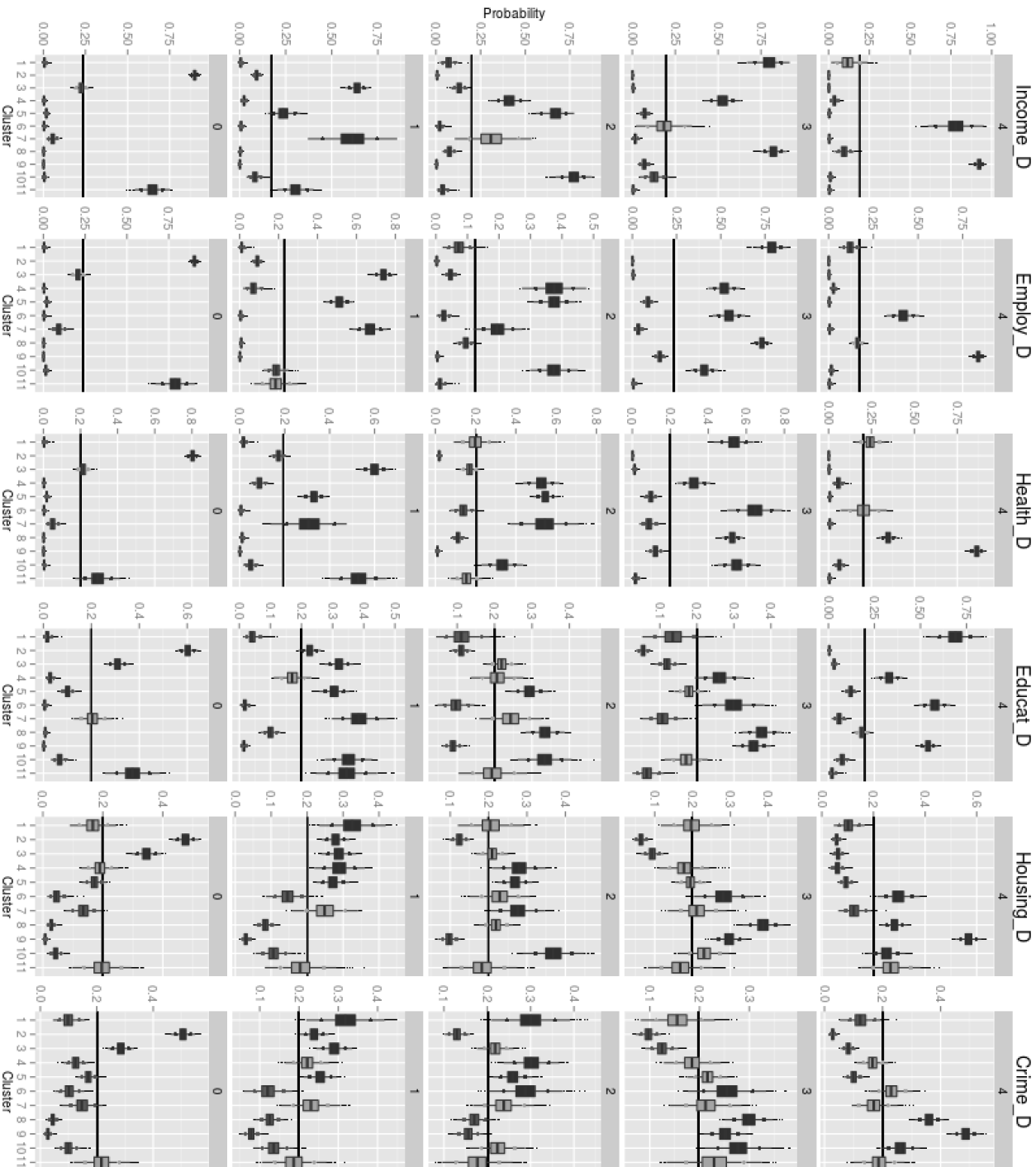
The cluster data are high-dimensional and complex. Figure 4 provides a visual representation of the parameters $\Phi_{c}$. Through the boxplots of the MCMC samples of the parameters $\Phi_{c}$, this figure provides also a representation of the uncertainty around these parameters. Each column $j$ in the figure represents $\Phi_{c,j,k}$, for $c=1,\ldots,11$ and $k=0,1,\ldots,4$ (the five quintiles of each covariate). Within a column $j$, each row $k$ is a visualisation of the boxplots for $\phi_{c,j,k}$ for each cluster $c$. This visual representation provides a further insight into the eleven clusters. We can identify patterns in the relationships between pollution and IMD domains at a glance. For example, Housing and Crime appear to generally increase as pollution levels increase, while the other domains show less linear patterns. We can also see here the details of the distributions of the levels of covariates that define the different clusters. Cluster 2 has the lowest levels of deprivation, although not the lowest levels of mean pollution. In contrast, cluster 9 has the highest levels of deprivation, and high levels of pollution, although not the highest among all clusters. The mean IMD per cluster highlights the complex relationship between IMD, pollution and deprivation. For example, for cluster 6, which has a high mean IMD, there is strong deprivation for the first four domains. However, the domains of Crime and Housing are rather evenly spread among all levels of the covariates, suggesting that they do not contribute to the deprivation that characterises these areas. This is an example of a complex pattern that cannot be identified when the domains are simply collapsed into the IMD.

Figure 5: Summary table of the clusters. The quintiles for pollution and each domain of the IMD are shown for each cluster.

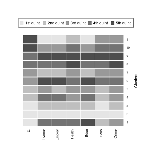
In Figure 5 we provide a summary of the posterior means for each cluster. Each row represents a cluster. The columns represents, respectively, the mean observed pollution and each domain of IMD. The colour of each column of the matrix corresponds to a quintile of the distribution of that variable. As before, the clusters are ordered by their observed pollution level. Note that the colours in the matrix do not become darker (or lighter) in a smooth manner. Together, Figure 5 and Figure 3 suggest that the areas of low pollution and low deprivation are in outer London. As we get closer to the centre, pollution increases and many of the deprivation variables increase levels. However, there are many notable exceptions to this. For example, cluster 11 has the highest levels of pollution, but among the lowest levels of deprivation. On the contrary, cluster 1 has the lowest level of pollution, but rather high levels of deprivation on all domains except Housing.

Figure 6: Posterior mean of the spatial conditional autoregressive term.

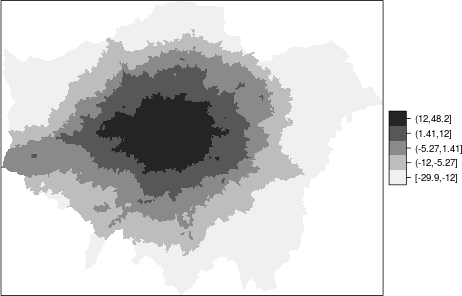
Figure 6 shows the posterior mean of the spatial term $\exp(u_{i})$ for each area, which accounts for the residual spatial variation in NOx after having adjusted for the cluster assignment. The map presents a clear pattern going from central London (darker) to outer London (lighter) with values ranging from -30 to 48 $\mu g/m^{3}$, thus suggesting that the model picks up the spatial dependence in air pollution concentration which is not explained by deprivation.

Figure 7: Beanplots of the posterior predictive distributions for these four pseudo profiles: $(0,0,0,0,0,0),(0,\text{NA},\text{NA},\text{NA},\text{NA},\text{NA}),(4,4,4,4,4,4),(4,4,4,4,4,0)$ where the elements of each vector represent respectively the IMD domains (Income, Employment, Health, Education, Housing, Crime).

We can explore the relationships between covariates and response further by looking at the posterior predictive distributions. The profile regression model allows us to predict the pollution level for specific combinations of the IMD domains. If we wish to understand the role of a particular covariate or group of covariates, we can specify a number of predictive scenarios (pseudo-profiles), that capture the range of possibilities for the covariates that we are interested in (Hastie et al., 2013). For each of these pseudo-profiles we can see how these would have been allocated in our mixture model to understand the level of pollution associated with them once we have accounted for the spatial residuals.

In Figure 7 we show beanplots of four pseudo-profiles: $(0,0,0,0,0,0)$, $(0,\text{NA},\text{NA},\text{NA},\text{NA},\text{NA})$, $(4,4,4,4,4,4)$, $(4,4,4,4,4,0)$. The elements of each vector represent the IMD domains in the following order: Income, Employment, Health, Education, Housing, Crime. Each of these beanplots shows the pseudo-profile corresponding to particular values of the IMD domain of interest for an average area (ie. including the mean spatial residual, which is 0). When ‘NA’ is set, this allows that domain to vary, de facto marginalising for it, i.e. capturing all possible values it can take. For example, the beanplot for the first pseudo-profile on the left presents the posterior predictive distribution of NOx for areas with the lowest levels of deprivation and shows values between 68 and 75$\mu$g/m³. Using this as benchmark we can make some comparisons: areas characterised by low Income and marginalising for the remaining domains (second beanplot from the left) have a much wider posterior predictive distribution, with values going from 67 to 78$\mu$g/m³ while areas with in the highest quintile of deprivation for all the domains (third beanplot from the left) present consistently highest level of pollution (ranging between 71 to 77$\mu$g/m³). The last beanplot shows the posterior predictive distribution of NOx in an area where crime has decreased to the first quintile (for instance through the implementation of a policy) while the other domains remains in the last quintile. Comparing it with the previous one it an be seen a similar distribution, but with a lower tail which could be a consequence of the policy implementation.

All predictive profiles can be computed and we provide here only these examples to show how these can be interpreted, if there was an interest in the posterior predictive distribution of specific combinations of deprivation levels, these could be explored in depth. Moreover, if there was interest in a specific area, the pseudo-profiles could be adjusted by adding the spatial residual.

5 Discussion

In this paper we have considered a spatially-correlated response variable and a set of highly correlated covariates. We have extended the profile regression model, a Bayesian clustering method used to deal with collinearity in the predictors, to account for spatial correlation adding a spatial conditionally autoregressive term.

We have applied our method to explain the relationship between air pollution and social deprivation in Greater London. The Index of Multiple Deprivation is commonly used as a proxy for deprivation, as its domains usually cannot be analysed individually due to the high correlation between them. We have illustrated how profile regression can produce meaningful and useful results which shed light on the complex non linear relationship between pollution and the different domains.

We want to stress that we are not framed in a standard regression approach, where the interest is to estimate the effect of each predictor on the outcome, as we do not attempt to explain the level of air pollution through the IMD domains. On the other hand through cluster assignment the profile regression is able to disentangle the complex relationship between IMD and air pollution; this method has the added benefit of providing readily available prediction estimates which can be used to evaluate how the response could change for specific combinations of the predictors, and which could be used to evaluate the effect of policies.

A limitation of our model is that in its present formulation the spatial structure is not included on the cluster allocation, thus it accounts for local spatial dependency in the response, but not in the covariates, which is an extension we are going to work on in the future.

Appendix A Sampling for the spatial ICAR parameters

We include details of the sampling algorithm for the spatial ICAR parameters for Gaussian and Poisson distributed response. We have implemented both in the R package PReMiuM.

A.1 Gaussian response

The conditional distribution for $u_{i}$ is given by

$$\log(p(u_{i}|u_{-i},\bm{\beta},\bm{\theta},\sigma_{Y}^{2},Z_{i},\tau,Y_{i},W_{i},T_{i})) \propto \log p(Y_{i}|u_{i},\bm{\beta},\theta,Z_{i},\sigma^{2}_{Y},W_{i},T_{i})+\log p(u_{i}|u_{-i},\tau)$$

$$\propto -\frac{1}{2\sigma_{Y}^{2}}(Y_{i}-(\theta_{Z_{i}}+W_{i}\bm{\beta}+u_{i}))^{2}-\frac{1}{2}\tau n_{i}(u_{i}-\bar{u}_{i})^{2}$$

$$\propto -\frac{1}{2\sigma^{2}_{i}}(u_{i}-m_{i})^{2}$$

with

$$\left\{\begin{array}[]{l}m_{i}=\frac{\frac{1}{\sigma_{Y}^{2}}(Y_{i}-\theta_{Z_{i}}-W_{i}\bm{\beta})-\tau n_{i}\bar{u}_{i}}{\frac{1}{\sigma_{Y}^{2}}+\tau n_{i}}\\ \sigma^{2}_{i}=\frac{1}{\frac{1}{\sigma_{Y}^{2}}+\tau n_{i}}\end{array}\right.$$

with , $\bar{u}_{i}=\frac{1}{n_{i}}\sum_{j\in\rho_{i}}u_{j}$ $\rho_{i}$ is the set of neighbours of $i$. Thus, for Normal response the prior is conjugated, the conjugated complete conditional distribution is Normal with mean $m_{i}$ and variance $\sigma_{i}^{2}$. The conditional distribution for $\tau$ is given by

$$\log(p(\tau|u))=(a_{\tau}+\frac{n-1}{2}-1)\log(\tau)-\tau(b_{\tau}+\frac{1}{2}u^{T}\mathbf{P}u)$$

Thus $\tau\sim\mbox{Gamma}(a_{\tau}+\frac{n-1}{2},b_{\tau}+\frac{1}{2}u^{T}\mathbf{P}u)$.

A.2 Poisson response

For Poisson response, suitable for count data, the likelihood is given by

$$f_{Y}(y_{i}|z_{i}=c,\theta_{c},\bm{\Lambda},W_{i})=p(Y_{i}|z_{i}=c,\theta_{c},\bm{\beta},u_{i},W_{i})=\frac{\mu_{i}^{Y_{i}}}{Y_{i}!}\exp\{-\mu_{i}\},$$

where each individual $i$ is associated with an expected offset $E_{i}$,

$$\mu_{i}=E_{i}\exp\{\lambda_{i}\},\;\;\;\textrm{for }\lambda_{i}=\theta_{Z_{i}}+\bm{\beta}^{\top}W_{i}.$$

As for the Gaussian response, the parameters $u=(u_{1},\cdots,u_{n})\sim N(0,\mathbf{\tau P})$ with $\mathbf{P}=\{P_{ij}\}$ a precision matrix such that

$$P_{ij}=\begin{cases}n_{i}&\mbox{if}\;i=j\\ -I\{i\sim j\}&\mbox{if}\;i\neq j\\ \end{cases}$$

where $n_{i}$ is the number of neighbours of subject $i$, $I$ is the indicator function and $i\sim j$ indicates that regions $i$ and $j$ are neighbours. The prior of $\tau$ is given by

$$\tau\sim\mbox{Gamma}(a_{\tau},b_{\tau})$$

such that

$$E(\tau)=\frac{a_{\tau}}{b_{\tau}}\quad and\quad\mbox{Var}(\tau)=\frac{a_{\tau}}{b_{\tau}^{2}}.$$

The conditional distribution for $u_{i}$ is given by

$$\log(p(u_{i}|u_{-i},\bm{\beta},\theta,Z,\tau,Y))=Y_{i}u_{i}-E_{i}\exp(X_{i}\bm{\beta}+\theta_{Z_{i}}+u_{i})-\frac{1}{2}\tau n_{i}(u_{i}-\bar{u}_{i})^{2}$$

with $\bar{u}_{i}=\frac{1}{n_{i}}\sum_{j\in\rho_{i}}u_{j}$ and $\rho_{i}$ is the set of neighbours of $i$. We implemented an adaptive rejection sampler for $u_{i}$. The conditional distribution for $\tau$ is given by

$$\log(p(\tau|u))=(a_{\tau}+\frac{n-1}{2}-1)\log(\tau)-\tau(b_{\tau}+\frac{1}{2}u^{T}\mathbf{P}u).$$

Thus $\tau\sim\mbox{Gamma}(a_{\tau}+\frac{n-1}{2},b_{\tau}+\frac{1}{2}u^{T}\mathbf{P}u)$.

References

- Abellan et al. (2008) Abellan, J., S. Richardson, and N. Best (2008). Use of space-time models to investigate the stability of patterns of disease. Environmental Health Perspectives 116, 1111–1119.
- Barcelo et al. (2009) Barcelo, M., M. Saez, and S. C. (2009). Spatial variability in mortality inequalities, socioeconomic deprivation, and air pollution in small areas of the barcelona metropolitan region, spain. Science of the Total Environment 407(21), 5501–5523.
- Benach et al. (2001) Benach, J., Y. Yasui, C. Borrell, M. Saez, and M. I. Pasarin (2001). Material deprivation and leading causes of death by gender: evidence from a nationwide small area study. Journal of Epidemiology and Community Health 55, 239–245.
- Besag et al. (1991) Besag, J., J. York, and A. Mollié (1991). Bayesian image restoration, with two applications in spatial statistics. Annals of the institute of statistical mathematics 43(1), 1–20.
- Bigelow and Dunson (2009) Bigelow, J. L. and D. B. Dunson (2009, March). Bayesian Semiparametric Joint Models for Functional Predictors. Journal of the American Statistical Association 104(485), 26–36.
- Blakely et al. (2004) Blakely, T., I. Kawachi, J. Atkinson, and J. Fawcett (2004). Income and mortality: the shape of the association and confounding new zealand census-mortality study. international Journal of Epidemiology 33, 874–883.
- Blakely and Woodward (2000) Blakely, T. and A. Woodward (2000). Ecological effects in multi-level studies. Journal of Epidemiology Community and Health 54, 367–374.
- Blowers and Leroy (1994) Blowers, A. and P. Leroy (1994). Power, politics and environmental inequality: A theoretical and empirical analysis of the process of peripheralisation. Environmental Politics 3, 197–228.
- Brown (1995) Brown, P. (1995). Race, class, and environmental health: a review and systematization of the literature. Environmental Research 69, 15–30.
- Brulle and Pellow (2006) Brulle, R. and D. Pellow (2006). Environmental justice: human health and environmental inequalities. Annual Review of Public Health 27, 103–124.
- Chen et al. (2008) Chen, H., M. Goldberg, and P. Villeneuve (2008). A systematic review of the relation between long-term exposure to ambient air pollution and chronic diseases. Reviews on Environmental Health 23, 243–297.
- Davidson and Anderton (2000) Davidson, P. and D. Anderton (2000). Demographics of dumping ii: a national environmental equity survey and the distribution of hazardous materials handlers. Demography 37, 461–466.
- Dunson et al. (2008) Dunson, D. B., A. B. Herring, and A. M. Siega-Riz (2008, December). Bayesian Inference on Changes in Response Densities Over Predictor Clusters. Journal of the American Statistical Association 103(484), 1508–1517.
- Elliott and Wartenberg (2004) Elliott, P. and D. Wartenberg (2004). Spatial epidemiology: current approaches and future challenges. Environmental Health Perspectives 112(9), 998–1006.
- Hastie et al. (2013) Hastie, D. I., S. Liverani, L. Azizi, S. Richardson, and I. Stücker (2013). A semi-parametric approach to estimate risk functions associated with multi-dimensional exposure profiles: application to smoking and lung cancer. BMC Medical Research Methodology 13(1), 129.
- Hastie et al. (2015) Hastie, D. I., S. Liverani, and S. Richardson (2015). Sampling from Dirichlet process mixture models with unknown concentration parameter: mixing issues in large data implementations. Statistics and Computing 25(5), 1023–1037.
- Higgs et al. (1998) Higgs, G., M. Senior, and H. Williams (1998). . spatial and temporal variation of mortality and deprivation. 1: widening health inequalities. Environment and Planning A 30(1), 661–682.
- Lantz et al. (2001) Lantz, P., J. Lynch, J. House, J. Lepkowski, R. Mero, M. Musick, and D. Williams (2001). . socioeconomic disparities in health change in a longitudinal study of us adults: the role of health-risk behaviors. Social Science and Medicine 53, 29–40.
- Laurent et al. (2007) Laurent, O., D. Bard, L. Filleul, and C. Segala (2007). Effect of socioeconomic status on the relationship between atmospheric pollution and mortality. Journal of Epidemiology and Community Health 61, 665–675.
- Leyland et al. (2007) Leyland, A., R. Dundas, P. Mcloone, and F. Boddy (2007). Cause-specific inequalities in mortality in scotland: two decades of change. a population-based study. BMC Public Health 7, 1–12.
- Li et al. (2012) Li, G., N. Best, A. Hansell, I. Ahmed, and S. Richardson (2012). Baystdetect: detecting unusual temporal patterns in small area data via bayesian model choice. Biostatistics 13(4), 695–710.
- Liverani et al. (2015) Liverani, S., D. I. Hastie, L. Azizi, M. Papathomas, and S. Richardson (2015). PReMiuM: An R package for Profile Regression Mixture Models using Dirichlet Processes. Journal of Statistical Software 64(7), 1–30.
- Marmot (2007) Marmot, M. (2007). Achieving health equity: from root causes to fair outcomes. Lancet 370, 1153–1163.
- Molitor et al. (2014) Molitor, J., I. J. Brown, Q. Chan, M. Papathomas, S. Liverani, N. Molitor, S. Richardson, L. Van Horn, M. L. Daviglus, A. Dyer, J. Stamler, P. Elliott, and I. R. Group (2014). Blood Pressure Differences Associated With Optimal Macronutrient Intake Trial for Heart Health (OMNIHEART)–Like Diet Compared With a Typical American Diet. Hypertension 64(6), 1198–1204.
- Molitor et al. (2010) Molitor, J., M. Papathomas, M. Jerrett, and S. Richardson (2010, July). Bayesian profile regression with an application to the National Survey of Children’s Health. Biostatistics 11(3), 484–498.
- Morello-Frosch and Jesdale (2006) Morello-Frosch, R. and B. Jesdale (2006). Separate and unequal: residential segregation and estimated cancer risks associated with ambient air toxics in u.s. metropolitan areas. Environmental Health Perspectives 114, 386–393.
- Morello-Frosch et al. (2002) Morello-Frosch, R., M. Pastor, C. Porras, and J. Sadd (2002). . separate and unequal: residential segregation and estimated cancer risks associated with ambient air toxics in u.s. metropolitan areas. Environmental Health Perspectives 110(2), 149–154.
- Morgenstern et al. (2007) Morgenstern, V., A. Zutavern, J. Cyrys, I. Brockow, U. Gehring, S. Koletzko, C. Bauer, D. Reinhardt, H. Wichmann, and J. Heinrich (2007). A case-control analysis of exposure to traffic and acute myocardial infarction. Occupational Environmental Medicine 64, 8–16.
- O’Neill et al. (2003) O’Neill, M., M. Jerrett, I. Kawachi, J. Levy, A. Cohen, N. Gouveia, P. Wilkinson, T. Fletcher, L. Cifuentes, and J. Schwartz (2003). Health, wealth, and air pollution: advancing theory and methods. Environmental Health Perspectives 111, 1861–1870.
- Papathomas et al. (2012) Papathomas, M., J. Molitor, C. Hoggart, D. Hastie, and S. Richardson (2012). Exploring data from genetic association studies using bayesian variable selection and the dirichlet process: application to searching for gene gene patterns. Genetic epidemiology 36(6), 663–674.
- Papathomas et al. (2011) Papathomas, M., J. Molitor, S. Richardson, E. Riboli, and P. Vineis (2011). Examining the joint effect of multiple risk factors using exposure risk profiles: lung cancer in nonsmokers. Environmental health perspectives 119(1), 84.
- Perlin et al. (1995) Perlin, S., R. Setzer, J. Creason, and K. Sexton (1995). Distribution of industrial air emissions by income and race in the united states: an approach using the toxic release inventory. Environmental Science and Technology 29, 69–80.
- Peters et al. (2004) Peters, A., S. Von Klot, M. Heier, I. Trentinaglia, A. Hormann, H. Wichmann, and H. Lowel (2004). A case-control analysis of exposure to traffic and acute myocardial infarction. New England Journal of Medicine 351, 1721–1730.
- Pirani et al. (2015) Pirani, M., N. Best, M. Blangiardo, S. Liverani, R. W. Atkinson, and G. W. Fuller (2015). Analysing the health effects of simultaneous exposure to physical and chemical properties of airborne particles. Environment International 79, 56–64.
- Pope et al. (2011) Pope, C., R. Burnett, M. Turner, A. Cohen, D. Krewski, M. Jerrett, S. Gapstur, and M. Thun (2011). Lung cancer and cardiovascular disease mortality associated with ambient air pollution and cigarette smoke: shape of the exposure-response relationships. Environmental Health Perspectives 119, 1616–1621.
- Tonne et al. (2007) Tonne, C., S. Melly, M. Mittleman, B. Coull, R. Goldberg, and J. Schwartz (2007). A case-control analysis of exposure to traffic and acute myocardial infarction. Environmental Health Perspectives 115, 53–57.