GW150914: First results from the search for binary black hole coalescence with Advanced LIGO
Abstract
On September 14, 2015 at 09:50:45 UTC the two detectors of the Laser Interferometer Gravitational-wave Observatory (LIGO) simultaneously observed the binary black hole merger GW150914. We report the results of a matched-filter search using relativistic models of compact-object binaries that recovered GW150914 as the most significant event during the coincident observations between the two LIGO detectors from September 12 to October 20, 2015. GW150914 was observed with a matched filter signal-to-noise ratio of and a false alarm rate estimated to be less than 1 event per years, equivalent to a significance greater than .
I Introduction
On September 14, 2015 at 09:50:45 UTC the LIGO Hanford, WA, and Livingston, LA, observatories detected a signal from the binary black hole merger GW150914 Abbott et al. (2016a). The initial detection of the event was made by low-latency searches for generic gravitational-wave transients Abbott et al. (2016b). We report the results of a matched-filter search using relativistic models of compact binary coalescence waveforms that recovered GW150914 as the most significant event during the coincident observations between the two LIGO detectors from September 12 to October 20, 2015. This is a subset of the data from Advanced LIGO’s first observational period that ended on January 12, 2016.
The binary coalescence search targets gravitational-wave emission from compact-object binaries with individual masses from 1 to 99 , total mass less than 100 and dimensionless spins up to 0.99. The search was performed using two independently implemented analyses, referred to as PyCBC Dal Canton et al. (2014); Usman et al. (2015); Nitz et al. (2016) and GstLAL Cannon et al. (2012); Privitera et al. (2014); Messick et al. (2016). These analyses use a common set of template waveforms Taracchini et al. (2014); Pürrer (2016); Capano et al. (2016), but differ in their implementations of matched filtering Allen et al. (2012); Cannon et al. (2010a), their use of detector data-quality information Abbott et al. (2016c), the techniques used to mitigate the effect of non-Gaussian noise transients in the detector Allen (2005); Cannon et al. (2012), and the methods for estimating the noise background of the search Usman et al. (2015); Cannon et al. (2015).
GW150914 was observed in both LIGO detectors Abbott et al. (2016d) with a time-of-arrival difference of 7 ms, which is less than the 10 ms inter-site propagation time, and a combined matched-filter signal to noise ratio (SNR) of . The search reported a false alarm rate estimated to be less than 1 event per years, equivalent to a significance greater than . The basic features of the GW150914 signal point to it being produced by the coalescence of two black holes Abbott et al. (2016a). The best-fit template parameters from the search are consistent with detailed parameter estimation that identifies GW150914 as a near-equal mass black hole binary system with source-frame masses and at the credible level Abbott et al. (2016e).
The second most significant candidate event in the observation period (referred to as LVT151012) was reported on October 12, 2015 at 09:54:43 UTC with a combined matched-filter SNR of . The search reported a false alarm rate of 1 per 2.3 years and a corresponding false alarm probability of 0.02 for this candidate event. Detector characterization studies have not identified an instrumental or environmental artifact as causing this candidate event Abbott et al. (2016c). However, its false alarm probability is not sufficiently low to confidently claim this candidate event as a signal Gonzalez et al. (2012e). Detailed waveform analysis of this candidate event indicates that it is also a binary black hole merger with source frame masses and , if it is of astrophysical origin.
This paper is organized as follows: Sec. II gives an overview of the compact binary coalescence search and the methods used. Sec. III and Sec. IV describe the construction and tuning of the two independently implemented analyses used in the search. Sec. V presents the results of the search, and follow-up of the two most significant candidate events, GW150914 and LVT151012.
II Search Description
The binary coalescence search Thorne (1987); Sathyaprakash and Dhurandhar (1991); Cutler et al. (1993); Finn (1992); Finn and Chernoff (1993); Dhurandhar and Sathyaprakash (1994); Balasubramanian et al. (1996); Flanagan and Hughes (1998) reported here targets gravitational waves from binary neutron stars, binary black holes, and neutron star–black hole binaries, using matched filtering Wainstein and Zubakov (1962) with waveforms predicted by general relativity. Both the PyCBC and GstLAL analyses correlate the detector data with template waveforms that model the expected signal. The analyses identify candidate events that are detected at both observatories consistent with the ms inter-site propagation time. Events are assigned a detection-statistic value that ranks their likelihood of being a gravitational-wave signal. This detection statistic is compared to the estimated detector noise background to determine the probability that a candidate event is due to detector noise.
We report on a search using coincident observations between the two Advanced LIGO detectors Aasi et al. (2015) in Hanford, WA (H1) and in Livingston, LA (L1) from September 12 to October 20, 2015. During these days, the detectors were in coincident operation for a total of 18.4 days. Unstable instrumental operation and hardware failures affected 20.7 hours of these coincident observations. These data are discarded and the remaining 17.5 days are used as input to the analyses Abbott et al. (2016c). The analyses reduce this time further by imposing a minimum length over which the detectors must be operating stably; this is different between the two analysis (2064 s for PyCBC and 512 s for GstLAL), as described in Sec. III and Sec. IV. After applying this cut, the PyCBC analysis searched of coincident data and the GstLAL analysis searched days of coincident data. To prevent bias in the results, the configuration and tuning of the analyses were determined using data taken prior to September 12, 2015.
A gravitational-wave signal incident on an interferometer alters its arm lengths by and , such that their measured difference is , where is the gravitational-wave metric perturbation projected onto the detector, and is the unperturbed arm length Abramovici et al. (1992). The strain is calibrated by measuring the detector’s response to test mass motion induced by photon pressure from a modulated calibration laser beam Abbott et al. (2016f). Changes in the detector’s thermal and alignment state cause small, time-dependent systematic errors in the calibration Abbott et al. (2016f). The calibration used for this search does not include these time-dependent factors. Appendix A demonstrates that neglecting the time-dependent calibration factors does not affect the result of this search.
The gravitational waveform depends on the chirp mass of the binary, Peters and Mathews (1963); Peters (1964), the symmetric mass ratio Blanchet et al. (1995), and the angular momentum of the compact objects Kidder et al. (1993); Kidder (1995) (the compact object’s dimensionless spin), where is the angular momentum of the compact objects. The effect of spin on the waveform depends also on the ratio between the component objects’ masses Blanchet (2014). Parameters which affect the overall amplitude and phase of the signal as observed in the detector are maximized over in the matched-filter search, but can be recovered through full parameter estimation analysis Abbott et al. (2016e). The search parameter space is therefore defined by the limits placed on the compact objects’ masses and spins. The minimum component masses of the search are determined by the lowest expected neutron star mass, which we assume to be Miller and Miller (2014). There is no known maximum black hole mass Belczynski et al. (2014), however we limit this search to binaries with a total mass less than . The LIGO detectors are sensitive to higher mass binaries, however; the results of searches for binaries that lie outside this search space will be reported in future publications.
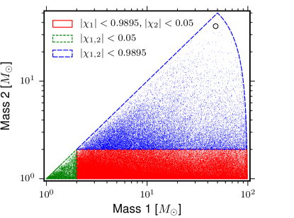
The limit on the spins of the compact objects are informed by radio and X-ray observations of compact-object binaries. The shortest observed pulsar period in a double neutron star system is ms Burgay et al. (2003), corresponding to a spin of . Observations of X-ray binaries indicate that astrophysical black holes may have near extremal spins McClintock et al. (2013). In constructing the search, we assume that compact objects with masses less than are neutron stars and we limit the magnitude of the component object’s spin to . For higher masses, the spin magnitude is limited to with the upper limit set by our ability to generate valid template waveforms at high spins Taracchini et al. (2014). At current detector sensitivity, limiting spins to for does not reduce the search sensitivity for sources containing neutron stars with spins up to , the spin of the fastest-spinning millisecond pulsar Lorimer (2008). Figure 1 shows the boundaries of the search parameter space in the component-mass plane, with the boundaries on the mass-dependent spin limits indicated.
Since the parameters of signals are not known in advance, each detector’s output is filtered against a discrete bank of templates that span the search target space Sathyaprakash and Dhurandhar (1991); Owen (1996); Owen and Sathyaprakash (1999); Babak et al. (2006); Cokelaer (2007). The placement of templates depends on the shape of the power spectrum of the detector noise. Both analyses use a low-frequency cutoff of Hz for the search. The average noise power spectral density of the LIGO detectors was measured over the period September 12 to September 26, 2015. The harmonic mean of these noise spectra from the two detectors was used to place a single template bank that was used for the duration of the search Keppel (2013); Usman et al. (2015). The templates are placed using a combination of geometric and stochastic methods Harry et al. (2009); Brown et al. (2012); Privitera et al. (2014); Capano et al. (2016) such that the loss in matched-filter SNR caused by its discrete nature is %. Approximately 250,000 template waveforms are used to cover this parameter space, as shown in Fig. 1.
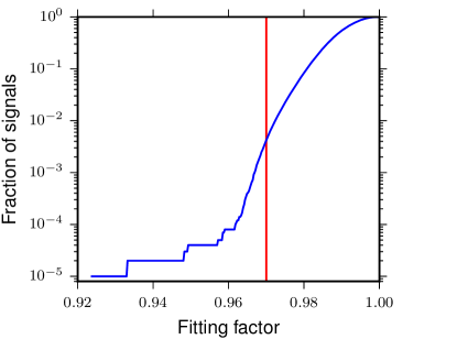
The performance of the template bank is measured by the fitting factor Apostolatos (1996); this is the fraction of the maximum signal-to-noise ratio that can be recovered by the template bank for a signal that lies within the region covered by the bank. The fitting factor is measured numerically by simulating a signal and determining the maximum recovered matched-filter SNR over the template bank. Figure 2 shows the resulting distribution of fitting factors obtained for the template bank over the observation period. The loss in matched-filter SNR is less than for more than % of the simulated signals.
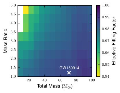
The template bank assumes that the spins of the two compact objects are aligned with the orbital angular momentum. The resulting templates can nonetheless effectively recover systems with misaligned spins in the parameter-space region of GW150914. To measure the effect of neglecting precession in the template waveforms, we compute the effective fitting factor which weights the fraction of the matched-filter SNR recovered by the amplitude of the signal Buonanno et al. (2003). When a signal with a poor orientation is projected onto the detector, the amplitude of the signal may be too small to detect even if there was no mismatch between the signal and the template; the weighting in the effective fitting accounts for this. Figure 3 shows the effective fitting factor for simulated signals from a population of simulated precessing binary black holes that are uniform in co-moving volume Pan et al. (2014); Harry et al. (2016). The effective fitting factor is lowest at high mass ratios and low total mass, where the effects of precession are more pronounced. In the region close to the parameters of GW150914 the aligned-spin template bank is sensitive to a large fraction of precessing signals Harry et al. (2016).
In addition to possible gravitational-wave signals, the detector strain contains a stationary noise background that primarily arises from photon shot noise at high frequencies and seismic noise at low frequencies. In the mid-frequency range, detector commissioning has not yet reached the point where test mass thermal noise dominates, and the noise at mid frequencies is poorly understood Abbott et al. (2016d, c); Martynov et al. (2016). The detector strain data also exhibits non-stationarity and non-Gaussian noise transients that arise from a variety of instrumental or environmental mechanisms. The measured strain is the sum of possible gravitational-wave signals and the different types of detector noise .
To monitor environmental disturbances and their influence on the detectors, each observatory site is equipped with an array of sensors Effler et al. (2015). Auxiliary instrumental channels also record the interferometer’s operating point and the state of the detector’s control systems. Many noise transients have distinct signatures, visible in environmental or auxiliary data channels that are not sensitive to gravitational waves. When a noise source with known physical coupling between these channels and the detector strain data is active, a data-quality veto is created that is used to exclude these data from the search Abbott et al. (2016c). In the GstLAL analysis, time intervals flagged by data quality vetoes are removed prior to the filtering. In the PyCBC analysis, these data quality vetoes are applied after filtering. A total of 2 hours is removed from the analysis by data quality vetoes. Despite these detector characterization investigations, the data still contains non-stationary and non-Gaussian noise which can affect the astrophysical sensitivity of the search. Both analyses implement methods to identify loud, short-duration noise transients and remove them from the strain data before filtering.
The PyCBC and GstLAL analyses calculate the matched-filter SNR for each template and each detector’s data Allen et al. (2012); Cannon et al. (2010b). In the PyCBC analysis, sources with total mass less than 4 are modeled by computing the inspiral waveform accurate to third-and-a-half post-Newtonian order Blanchet et al. (1995); Droz et al. (1999); Blanchet et al. (2004). To model systems with total mass larger than 4 , we use templates based on the effective-one-body (EOB) formalism Buonanno and Damour (2000), which combines results from the Post-Newtonian approach Blanchet et al. (1995, 2004) with results from black hole perturbation theory and numerical relativity Taracchini et al. (2014); Pürrer (2014) to model the complete inspiral, merger and ringdown waveform. The waveform models used assume that the spins of the merging objects are aligned with the orbital angular momentum. The GstLAL analysis uses the same waveform families, but the boundary between Post-Newtonian and EOB models is set at . Both analyses identify maxima of the matched-filter SNR (triggers) over the signal time of arrival.
To suppress large SNR values caused by non-Gaussian detector noise, the two analyses calculate additional tests to quantify the agreement between the data and the template. The PyCBC analysis calculates a chi-squared statistic to test whether the data in several different frequency bands are consistent with the matching template Allen (2005). The value of the chi-squared statistic is used to compute a re-weighted SNR for each maxima. The GstLAL analysis computes a goodness-of-fit between the measured and expected SNR time series for each trigger. The matched-filter SNR and goodness-of-fit values for each trigger are used as parameters in the GstLAL ranking statistic.
Both analyses enforce coincidence between detectors by selecting trigger pairs that occur within a ms window and come from the same template. The ms window is determined by the ms inter-site propagation time plus ms for uncertainty in arrival time of weak signals. The PyCBC analyses discards any triggers that occur during the time of data-quality vetoes prior to computing coincidence. The remaining coincident events are ranked based on the quadrature sum of the re-weighted SNR from both detectors Usman et al. (2015). The GstLAL analysis ranks coincident events using a likelihood ratio that quantifies the probability that a particular set of concident trigger parameters is due to a signal versus the probability of obtaining the same set of parameters from noise Cannon et al. (2012).
The significance of a candidate event is determined by the search background. This is the rate at which detector noise produces events with a detection-statistic value equal to or higher than the candidate event (the false alarm rate). Estimating this background is challenging for two reasons: the detector noise is non-stationary and non-Gaussian, so its properties must be empirically determined; and it is not possible to shield the detector from gravitational waves to directly measure a signal-free background. The specific procedure used to estimate the background is different for the two analyses.
To measure the significance of candidate events, the PyCBC analysis artificially shifts the timestamps of one detector’s triggers by an offset that is large compared to the inter-site propagation time, and a new set of coincident events is produced based on this time-shifted data set. For instrumental noise that is uncorrelated between detectors this is an effective way to estimate the background. To account for the search background noise varying across the target signal space, candidate and background events are divided into three search classes based on template length. To account for having searched multiple classes, the measured significance is decreased by a trials factor equal to the number of classes Lyons (2008).
The GstLAL analysis measures the noise background using the distribution of triggers that are not coincident in time. To account for the search background noise varying across the target signal space, the analysis divides the template bank into 248 bins. Signals are assumed to be equally likely across all bins and it is assumed that noise triggers are equally likely to produce a given SNR and goodness-of-fit value in any of the templates within a single bin. The estimated probability density function for the likelihood statistic is marginalized over the template bins and used to compute the probability of obtaining a noise event with a likelihood value larger than that of a candidate event.
The result of the independent analyses are two separate lists of candidate events, with each candidate event assigned a false alarm probability and false alarm rate. These quantities are used to determine if a gravitational-wave signal is present in the search. Simulated signals are added to the input strain data to validate the analyses, as described in Appendix B.
III PyCBC Analysis
The PyCBC analysis Dal Canton et al. (2014); Usman et al. (2015); Nitz et al. (2016) uses fundamentally the same methods Brown et al. (2004); Allen et al. (2012); Allen (2005); Brown (2005); Babak et al. (2013); Brown et al. (2006); Deelman et al. (2005, 2015); Thain et al. (2005); Couvares et al. (2006); Jones et al. (01); Walt et al. (2011); Hunter (2007) as those used to search for gravitational waves from compact binaries in the initial LIGO and Virgo detector era Abbott et al. (2004, 2005a, 2005b, 2006, 2008a, 2008b, 2009a, 2009b); Abadie et al. (2010, 2012); Aasi et al. (2013, 2014), with the improvements described in Refs. Dal Canton et al. (2014); Usman et al. (2015). In this Section, we describe the configuration and tuning of the PyCBC analysis used in this search. To prevent bias in the search result, the configuration of the analysis was determined using data taken prior to the observation period searched. When GW150914 was discovered by the low-latency transient searches Abbott et al. (2016a), all tuning of the PyCBC analysis was frozen to ensure that the reported false alarm probabilities are unbiased. No information from the low-latency transient search is used in this analysis.
Of the 17.5 days of data that are used as input to the analysis, the PyCBC analysis discards times for which either of the LIGO detectors is in their observation state for less than s; shorter intervals are considered to be unstable detector operation by this analysis and are removed from the observation time. After discarding time removed by data-quality vetoes and periods when detector operation is considered unstable the observation time remaining is .
For each template and for the strain data from a single detector , the analysis calculates the square of the matched-filter SNR defined by Allen et al. (2012)
| (1) |
where the correlation is defined by
| (2) |
where is the Fourier transform of the time domain quantity given by
| (3) |
The quantity is the one-sided average power spectral density of the detector noise, which is re-calculated every 2048 s (in contrast to the fixed spectrum used in template bank construction). Calculation of the matched-filter SNR in the frequency domain allows the use of the computationally efficient Fast Fourier Transform int (2015); Frigo and Johnson (2005). The square of the matched-filter SNR in Eq. (1) is normalized by
| (4) |
so that its mean value is , if contains only stationary noise Cutler and Flanagan (1994).
Non-Gaussian noise transients in the detector can produce extended periods of elevated matched-filter SNR that increase the search background Usman et al. (2015). To mitigate this, a time-frequency excess power (burst) search Robinet (2015) is used to identify high-amplitude, short-duration transients that are not flagged by data-quality vetoes. If the burst search generates a trigger with a burst SNR exceeding , the PyCBC analysis vetoes these data by zeroing out s of centered on the time of the trigger. The data is smoothly rolled off using a Tukey window during the s before and after the vetoed data. The threshold of is chosen to be significantly higher than the burst SNR obtained from plausible binary signals. For comparison, the burst SNR of GW150914 in the excess power search is . A total of burst-transient vetoes are produced in the two detectors, resulting in s of data removed from the search. A time-frequency spectrogram of the data at the time of each burst-transient veto was inspected to ensure that none of these windows contained the signature of an extremely loud binary coalescence.
The analysis places a threshold of on the single-detector matched-filter SNR and identifies maxima of with respect to the time of arrival of the signal. For each maximum we calculate a chi-squared statistic to determine whether the data in several different frequency bands are consistent with the matching template Allen (2005). Given a specific number of frequency bands , the value of the reduced is given by
| (5) |
where is the sub-template corresponding to the -th frequency band. Values of near unity indicate that the signal is consistent with a coalescence. To suppress triggers from noise transients with large matched-filter SNR, is re-weighted by Abadie et al. (2012); Babak et al. (2013)
| (6) |
Triggers that have a re-weighted SNR or that occur during times subject to data-quality vetoes are discarded.
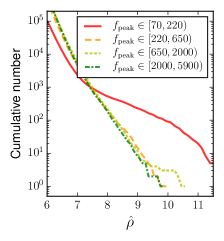
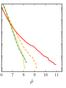
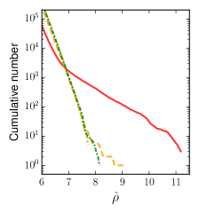
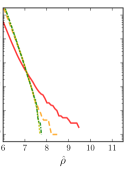
The template waveforms span a wide region of time-frequency parameter space and the susceptibility of the analysis to a particular type of noise transient can vary across the search space. This is demonstrated in Fig. 4 which shows the cumulative number of noise triggers as a function of re-weighted SNR for Advanced LIGO engineering run data taken between September 2 and September 9, 2015. The response of the template bank to noise transients is well characterized by the gravitational-wave frequency at the template’s peak amplitude, . Waveforms with a lower peak frequency have less cycles in the detector’s most sensitive frequency band from – Hz Abbott et al. (2016d); Martynov et al. (2016), and so are less easily distinguished from noise transients by the re-weighted SNR.
The number of bins in the test is a tunable parameter in the analysis Usman et al. (2015). Previous searches used a fixed number of bins Babak et al. (2005) with the most recent Initial LIGO and Virgo searches using bins for all templates Abadie et al. (2012); Aasi et al. (2013). Investigations on data from LIGO’s sixth science run Nitz (2015); Aasi et al. (2013) showed that better noise rejection is achieved with a template-dependent number of bins. The left two panels of Fig. 4 show the cumulative number of noise triggers with bins used in the test. Empirically, we find that choosing the number of bins according to
| (7) |
gives better suppression of noise transients in Advanced LIGO data, as shown in the right panels of Fig. 4.
The PyCBC analysis enforces signal coincidence between detectors by selecting trigger pairs that occur within a ms window and come from the same template. We rank coincident events based on the quadrature sum of the from both detectors Usman et al. (2015). The final step of the analysis is to cluster the coincident events, by selecting those with the largest value of in each time window of s. Any other events in the same time window are discarded. This ensures that a loud signal or transient noise artifact gives rise to at most one candidate event Usman et al. (2015).
The significance of a candidate event is determined by the rate at which detector noise produces events with a detection-statistic value equal to or higher than that of the candidate event. To measure this, the analysis creates a “background data set” by artificially shifting the timestamps of one detector’s triggers by many multiples of s and computing a new set of coincident events. Since the time offset used is always larger than the time-coincidence window, coincident signals do not contribute to this background. Under the assumption that noise is not correlated between the detectors Abbott et al. (2016c), this method provides an unbiased estimate of the noise background of the analysis.
To account for the noise background varying across the target signal space, candidate and background events are divided into different search classes based on template length. Based on empirical tuning using Advanced LIGO engineering run data taken between September 2 and September 9, 2015, we divide the template space into three classes according to: (i) ; (ii) and Hz; (iii) and Hz. The significance of candidate events is measured against the background from the same class. For each candidate event, we compute the false alarm probability . This is the probability of finding one or more noise background events in the observation time with a detection-statistic value above that of the candidate event, given by Usman et al. (2015); Capano et al. (2016)
| (8) |
where is the observation time of the search, is the background time, and is the number of noise background triggers above the candidate event’s re-weighted SNR .
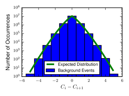
Eq. (8) is derived assuming Poisson statistics for the counts of time-shifted background events, and for the count of coincident noise events in the search Usman et al. (2015); Capano et al. (2016). This assumption requires that different time-shifted analyses (i.e. with different relative shifts between detectors) give independent realizations of a counting experiment for noise background events. We expect different time shifts to yield independent event counts since the s offset time is greater than the ms gravitational-wave travel time between the sites plus the ms autocorrelation length of the templates. To test the independence of event counts over different time shifts over this observation period, we compute the differences in the number of background events having between consecutive time shifts. Figure 5 shows that the measured differences on these data follow the expected distribution for the difference between two independent Poisson random variables Skellam (1946), confirming the independence of time shifted event counts.
If a candidate event’s detection-statistic value is larger than that of any noise background event, as is the case for GW150914, then the PyCBC analysis places an upper bound on the candidate’s false alarm probability. After discarding time removed by data-quality vetoes and periods when the detector is in stable operation for less than seconds, the total observation time remaining is . Repeating the time-shift procedure times on these data produces a noise background analysis time equivalent to years. Thus, the smallest false alarm probability that can be estimated in this analysis is approximately . Since we treat the search parameter space as 3 independent classes, each of which may generate a false positive result, this value should be multiplied by a trials factor or look-elsewhere effect Lyons (2008) of 3, resulting in a minimum measurable false alarm probability of . The results of the PyCBC analysis are described in Sec. V.
IV GstLAL Analysis
The GstLAL Gst (2016) analysis implements a time-domain matched filter search Cannon et al. (2012) using techinques that were developed to perform the near real-time compact-object binary searches Privitera et al. (2014); Messick et al. (2016). To accomplish this, the data and templates are each whitened in the frequency domain by dividing them by an estimate of the power spectral density of the detector noise. An estimate of the stationary noise amplitude spectrum is obtained with a combined median–geometric-mean modification of Welch’s method Messick et al. (2016). This procedure is applied piece-wise on overlapping Hann-windowed time-domain blocks that are subsequently summed together to yield a continuous whitened time series . The time-domain whitened template is then convolved with the whitened data to obtain the matched-filter SNR time series for each template. By the convolution theorem, obtained in this manner is the same as the obtained by frequency domain filtering in Eq. (1).
Of the 17.5 days of data that are used as input to the analysis, the GstLAL analysis discards times for which either of the LIGO detectors is in their observation state for less than s in duration. Shorter intervals are considered to be unstable detector operation by this analysis and are removed from the observation time. After discarding time removed by data-quality vetoes and periods when the detector operation is considered unstable the observation time remaining is days. To remove loud, short-duration noise transients, any excursions in the whitened data that are greater than are removed with 0.25 s padding. The intervals of vetoed in this way are replaced with zeros. The cleaned whitened data is the input to the matched filtering stage.
Adjacent waveforms in the template bank are highly correlated. The GstLAL analysis takes advantage of this to reduce the computational cost of the time-domain correlation. The templates are grouped by chirp mass and spin into 248 bins of templates each. Within each bin, a reduced set of orthonormal basis functions is obtained via a singular value decomposition of the whitened templates. We find that the ratio of the number of orthonormal basis functions to the number of input waveforms is 0.01 – 0.10, indicating a significant redundancy in each bin. The set of in each bin is convolved with the whitened data; linear combinations of the resulting time series are then used to reconstruct the matched-filter SNR time series for each template. This decomposition allows for computationally-efficient time-domain filtering and reproduces the frequency-domain matched filter to within 0.1% Cannon et al. (2010b, 2012, 2011).
Peaks in the matched-filter SNR for each detector and each template are identified over s windows. If the peak is above a matched-filter SNR of 4, it is recorded as a trigger. For each trigger, the matched-filter SNR time series around the trigger is checked for consistency with a signal by comparing the template’s autocorrelation function to the matched-filter SNR time series . The residual found after subtracting the autocorrelation function forms a goodness-of-fit test,
| (9) |
where is the time at the peak matched-filter SNR , and is a tunable parameter. A suitable value for was found to be 85.45 ms (175 samples at a Hz sampling rate). The quantity normalizes such that a well-fit signal has a mean value of in Gaussian noise Messick et al. (2016). The value is recorded with the trigger.
Each trigger is checked for time coincidence with triggers from the same template in the other detector. If two triggers occur from the same template within ms in both detectors, a coincident event is recorded. Coincident events are ranked according to a multidimensional likelihood ratio Cannon (2008); Cannon et al. (2015), then clustered in a s time window. The likelihood ratio ranks candidate events by the ratio of the probability of observing matched-filter SNR and from signals () versus obtaining the same parameters from noise (). Since the orthonormal filter decomposition already groups templates into regions with high overlap, we expect templates in each group to respond similarly to noise. We use the template group as an additional parameter in the likelihood ratio to account for how different regions of the compact binary parameter space are affected differently by noise processes. The likelihood ratio is thus:
| (10) |
where are the matched-filter SNR and in each detector, and is a parameter that measures the distance sensitivity of the given detector during the time of a trigger.
The numerator of the likelihood ratio is generated using an astrophysical model of signals distributed isotropically in the nearby Universe to calculate the joint SNR distribution in the two detectors Cannon et al. (2015). The distribution for the signal hypothesis assumes that the signal agrees to within of the template waveform and that the nearby noise is Gaussian. We assume all are equally likely for signals.
The noise is assumed to be uncorrelated between detectors. The denominator of the likelihood ratio therefore factors into the product of the distribution of noise triggers in each detector, . We estimate these using a two-dimensional kernel density estimation Silverman (1998) constructed from all of the single-detector triggers not found in coincidence in a single bin.
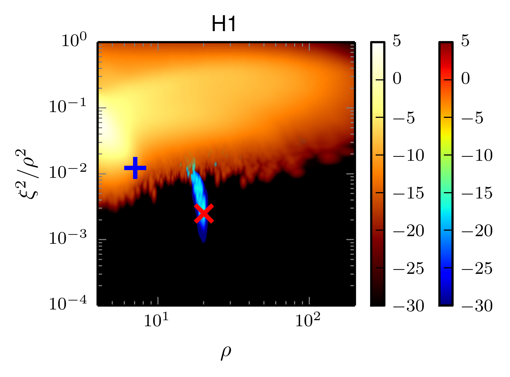
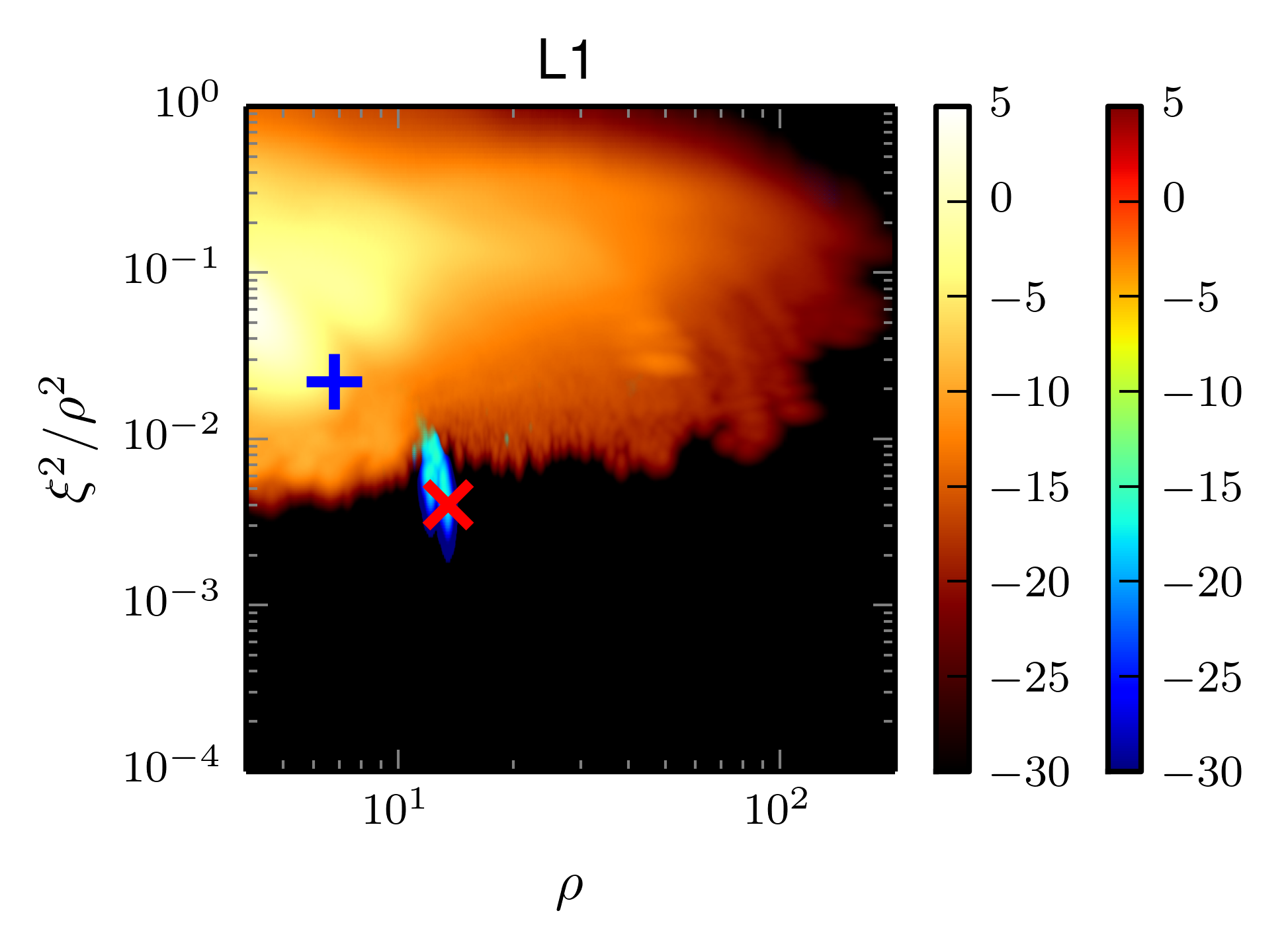
The likelihood ratio provides a ranking of events such that larger values of are associated with a higher probability of the data containing a signal. The likelihood ratio itself is not the probability that an event is a signal, nor does it give the probability that an event was caused by noise. Computing the probability that an event is a signal requires additional prior assumptions. Instead, for each candidate event, we compute the false alarm probability . This is the probability of finding one or more noise background events with a likelihood-ratio value greater than or equal to that of the candidate event. Assuming Poisson statistics for the background, this is given by:
| (11) |
Instead of using time shifts, the GstLAL anlysis estimates the Poisson rate of background events as:
| (12) |
where is the number of coincident events found above threshold in the analysis time , and is the probability of obtaining one or more events from noise with a likelihood ratio (the survival function). We find this by estimating the survival function in each template bin, then marginalize over the bins; i.e., . In a single bin, the survival function is
| (13) |
Here, are estimates of the distribution of triggers in each detector including all of the single-detector triggers, whereas the estimate of includes only those triggers which were not coincident. This is consistent with the assumption that the false alarm probability is computed assuming all events are noise.
The integration region is the volume of the four-dimensional space of for which the likelihood ratios are less than . We find this by Monte Carlo integration of our estimates of the single-detector noise distributions . This is approximately equal to the number of coincidences that can be formed from the single-detector triggers with likelihood ratios divided by the total number of possible coincidences. We therefore reach a minimum possible estimate of the survival function, without extrapolation, at the for which , where are the total number of triggers in each detector in the th bin.
GW150914 was more significant than any other combination of triggers. For that reason, we are interested in knowing the minimum false alarm probability that can be computed by the GstLAL analysis. All of the triggers in a template bin, regardless of the template from which they came, are used to construct the single-detector probability density distributions within that bin. The false alarm probability estimated by the GstLAL analysis is the probability that noise triggers occur within a ms time window and occur in the same template. Under the assumption that triggers are uniformly distributed over the bins, the minimum possible false alarm probability that can be computed is , where is the number of bins used, is the total number of triggers in , and is the total number of triggers in . For the present analysis, , , and is 248, yielding a minimum value of the false alarm probability of .
We cannot rule out the possibility that noise produced by the detectors violates the assumption that it is uniformly distributed among the templates within a bin. If we consider a more conservative noise hypothesis that does not assume that triggers are uniformly distributed within a bin and instead considers each template as a separate bin, we can evaluate the minimum upper bound on the false alarm probability of GW150914. This assumption would produce a larger minimum false alarm probability value by approximately the ratio of the number of templates to the present number of bins. Under this noise hypothesis, the minimum value of the false alarm probability would be , which is consistent with the minimum false alarm probability bound of the PyCBC analysis.
Figure 6 shows and in the warm colormap. The cool colormap includes triggers that are also found in coincidence, i.e., and , which is the probability density function used to estimate . It has been masked to only show regions which are not consistent with and . In both cases has been marginalized over in order to show all the data on a single figure. The positions of the two loudest events, described in the next section, are shown. Figure 6 shows that GW150914 falls in a region without any non-coincident triggers from any bin.
V Search Results
GW150914 was observed on September 14, 2015 at 09:50:45 UTC as the most significant event by both analyses. The individual detector triggers from GW150914 occurred within the 10 ms inter-site propagation time with a combined matched-filter SNR of . Both pipelines report the same matched-filter SNR for the individual detector triggers in the Hanford detector () and the Livingston detector (). GW150914 was found with the same template in both analyses with component masses and . The effective spin of the best-matching template is , where are the spins of the compact objects and is the direction of the binary’s orbital angular momentum. Due to the discrete nature of the template bank, follow-up parameter estimation is required to accurately determine the best fit masses and spins of the binary’s components Veitch et al. (2015); Abbott et al. (2016e).
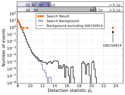
The frequency at peak amplitude of the best-matching template is Hz, placing it in noise-background class (iii) of the PyCBC analysis. Figure 7 (left) shows the result of the PyCBC analysis for this search class. In the time-shift analysis used to create the noise background estimate for the PyCBC analysis, a signal may contribute events to the background through random coincidences of the signal in one detector with noise in the other detector Capano et al. (2016). This can be seen in the background histogram shown by the black line. The tail is due to coincidence between the single-detector triggers from GW150914 and noise in the other detector. If a loud signal is in fact present, these random time-shifted coincidences contribute to an overestimate of the noise background and a more conservative assessment of the significance of an event. Figure 7 (left) shows that GW150914 has a re-weighted SNR , greater than all background events in its class. This value is also greater than all background in the other two classes. As a result, we can only place an upper bound on the false alarm rate, as described in Sec. III. This bound is equal to the number of classes divided by the background time . With classes and years, we find the false alarm rate of GW150914 to be less than . With an observing time of , the false alarm probability is . Converting this false alarm probability to single-sided Gaussian standard deviations according to , where is the inverse error function, the PyCBC analysis measures the significance of GW150914 as greater than .
| Event | Time (UTC) | FAR (yr-1) | (Mpc) | |||||
|---|---|---|---|---|---|---|---|---|
| GW150914 | 14 September 2015 09:50:45 |
|
||||||
| LVT151012 | 12 October 2015 09:54:43 |
|
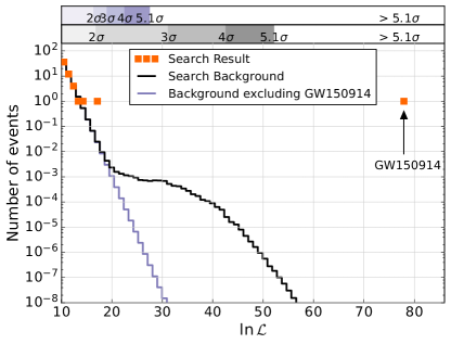
The GstLAL analysis reported a detection-statistic value for GW150914 of , as shown in the right panel of Fig. 7. The GstLAL analysis estimates the false alarm probability assuming that noise triggers are equally likely to occur in any of the templates within a background bin. However, as stated in Sec. IV, if the distribution of noise triggers is not uniform across templates, particularly in the part of the bank where GW150914 is observed, the minimum false alarm probability would be higher. For this reason we quote the more conservative PyCBC bound on the false alarm probability of GW150914 here and in Ref. Abbott et al. (2016a). However, proceeding under the assumption that the noise triggers are equally likely to occur in any of the templates within a background bin, the GstLAL analysis estimates the false alarm probability of GW150914 to be . The significance of GW150914 measured by GstLAL is consistent with the bound placed by the PyCBC analysis and provides additional confidence in the discovery of the signal.
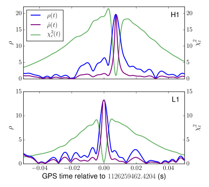
The difference in time of arrival between the Livingston and Hanford detectors from the individual triggers in the PyCBC analysis is ms, consistent with the time delay of ms recovered by parameter estimation Abbott et al. (2016e). Figure 8 (left) shows the matched-filter SNR , the -statistic, and the re-weighted SNR for the best-matching template over a period of ms around the time of GW150914 (we take the PyCBC trigger time in L1 as a reference). The matched-filter SNR peaks in both detectors at the time of the event and the value of the reduced chi-squared statistic is and at the time of the event, indicating an excellent match between the template and the data. The re-weighted SNR of the individual detector triggers of and are larger than that of any other single-detector triggers in the analysis; therefore the significance measurement of set using the s time shifts is a conservative bound on the false alarm probability of GW150914.
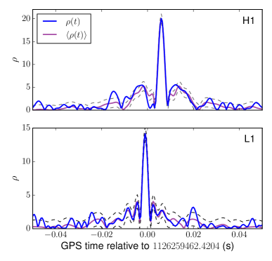
Figure 8 (right) shows ms of the GstLAL matched-filter SNR time series from each detector around the event time together with the predicted SNR time series computed from the autocorrelation function of the best-fit template. The difference between the autocorrelation and the observed matched-filter SNR is used to perform the GstLAL waveform-consistency test. The autocorrelation matches the observed matched-filter SNR extremely well, with consistency test values of and . No other triggers with comparable matched-filter SNR had such low values of the signal-consistency test during the entire observation period.
Both analyses have shown that the probability that GW150914 was formed by random coincidence of detector noise is extremely small. We therefore conclude that GW150914 is a gravitational-wave signal. To measure the signal parameters, we use parameter estimation methods that assume the presence of a coherent coalescing binary signal in the data from both detectors Veitch et al. (2015); Abbott et al. (2016e). Two waveform models were used which included inspiral, merger and ring-down portions of the signal: one which includes spin components aligned with orbital angular momentum Pan et al. (2010); Pürrer (2014) and one which includes the dominant modulation of the signal due to orbital precession caused by mis-aligned spins Hannam et al. (2014); Khan et al. (2016). The parameter estimates are described by a continuous probability density function over the source parameters. We conclude that GW150914 is a nearly equal mass black-hole binary system of source-frame masses and (median and credible range). The spin magnitude of the primary black hole is constrained to be less than with probability. The most stringent constraint on the spins of the two black holes is on the effective spin parameter . The parameters of the best-fit template are consistent with these values, given the discrete nature of the template bank. We estimate GW150914 to be at a luminosity distance of , which corresponds to a redshift . Full details of the source parameters for GW150914 are given in Ref. Abbott et al. (2016e) and summarized in Table 1.
When an event is confidently identified as a real gravitational wave signal, as for GW150914, the background used to determine the significance of other events is re-estimated without the contribution of this event. This is the background distribution shown as purple lines in Fig. 7. Both analyses reported a candidate event on October 12, 2015 at 09:54:43 UTC as the second-loudest event in the observation period, which we refer to as LVT151012. This candidate event has a combined matched-filter SNR of . The PyCBC analysis reported a false alarm rate of 1 per 2.3 years and a corresponding false alarm probability of 0.02 for this event. The GstLAL analysis reported a false alarm rate of 1 per years and a false alarm probability of . These results are consistent with expectations for candidate events with low matched-filter SNR, since PyCBC and GstLAL use different ranking statistics and background estimation methods. Detector characterization studies have not identified an instrumental or environmental artifact as causing this candidate event Abbott et al. (2016c), however its false alarm probability is not sufficiently low to confidently claim the event as a signal. It is significant enough to warrant follow-up, however. The results of signal parameter estimation, shown in Table 1, indicate that if LVT151012 is of astrophysical origin, then the source would be a stellar-mass binary black hole system with source-frame component masses and . The effective spin would be and the distance Mpc.
VI Conclusion
The LIGO detectors have observed gravitational waves from the merger of two stellar-mass black holes. The binary coalescence search detects GW150914 with a significance greater than during the observations reported. This result is confirmed by two independent matched filter analyses, providing confidence in the discovery. Detailed parameter estimation for GW150914 is reported in Ref. Abbott et al. (2016e), the implications for the rate of binary black hole coalescences in Ref. Abbott et al. (2016g), and tests for consistency of the signal with general relativity in Ref. Abbott et al. (2016h). Ref. Abbott et al. (2016i) discusses the astrophysical implications of this discovery. Full results of the compact binary search in Advanced LIGO’s first observing run will be reported in a future publication.
Acknowledgements.
The authors gratefully acknowledge the support of the United States National Science Foundation (NSF) for the construction and operation of the LIGO Laboratory and Advanced LIGO as well as the Science and Technology Facilities Council (STFC) of the United Kingdom, the Max-Planck-Society (MPS), and the State of Niedersachsen/Germany for support of the construction of Advanced LIGO and construction and operation of the GEO 600 detector. Additional support for Advanced LIGO was provided by the Australian Research Council. The authors gratefully acknowledge the Italian Istituto Nazionale di Fisica Nucleare (INFN), the French Centre National de la Recherche Scientifique (CNRS) and the Foundation for Fundamental Research on Matter supported by the Netherlands Organisation for Scientific Research, for the construction and operation of the Virgo detector and the creation and support of the EGO consortium. The authors also gratefully acknowledge research support from these agencies as well as by the Council of Scientific and Industrial Research of India, Department of Science and Technology, India, Science & Engineering Research Board (SERB), India, Ministry of Human Resource Development, India, the Spanish Ministerio de Economía y Competitividad, the Conselleria d’Economia i Competitivitat and Conselleria d’Educació, Cultura i Universitats of the Govern de les Illes Balears, the National Science Centre of Poland, the European Commission, the Royal Society, the Scottish Funding Council, the Scottish Universities Physics Alliance, the Hungarian Scientific Research Fund (OTKA), the Lyon Institute of Origins (LIO), the National Research Foundation of Korea, Industry Canada and the Province of Ontario through the Ministry of Economic Development and Innovation, the National Science and Engineering Research Council Canada, Canadian Institute for Advanced Research, the Brazilian Ministry of Science, Technology, and Innovation, Russian Foundation for Basic Research, the Leverhulme Trust, the Research Corporation, Ministry of Science and Technology (MOST), Taiwan and the Kavli Foundation. The authors gratefully acknowledge the support of the NSF, STFC, MPS, INFN, CNRS and the State of Niedersachsen/Germany for provision of computational resources.Appendix A Detector Calibration
The LIGO detectors do not directly record the strain signal, rather they sense power fluctuations in the light at the interferometer’s readout port Aasi et al. (2015). This error signal is used to generate a feedback signal to the detector’s differential arm length to maintain destructive interference of the light moving towards the readout port Abbott et al. (2016d). The presence of this feedback signal suppresses the length change from external sources; a combination of the error and control signals is used to estimate the detector strain. The strain is calibrated by measuring the detector’s response to test mass motion induced by photon pressure from a modulated calibration laser beam. Changes in the detector’s thermal and alignment state cause small, time-dependent systematic errors in the calibration. For more details see Ref. Abbott et al. (2016f).
Errors in the calibrated strain data lead to mismatches between waveform templates and the gravitational-wave signal. This mismatch has been shown to decrease the expected SNR , but only has a weak, quadratic dependence on calibration errors Allen (1996); Brown (for the LIGO Scientific Collaboration). However, the quantity used for detection is the re-weighted SNR for each detector. In this appendix, we analyze the impact of calibration errors on for signals similar to GW150914, and we find that the expected re-weighted SNR also shows only a weak dependence on calibration errors.
In the frequency domain, the process of calibration reconstructs the gravitational-wave strain from the differential arm length error signal , which is the filtered output of the photodiode. The function that relates the two quantities is the response function
| (14) |
This response function is constructed from the sensing transfer function that describes the frequency response of the detector to changes in the arm lengths as well as the actuation transfer function that describes the motion of the test mass when driven by the control signal to maintain destructive interference in the interferometer Abbott et al. (2016f).
The initial sensing and actuation transfer functions, measured before the start of the observing run, are defined by and respectively. However, over the course of an observing run, the frequency dependence of these transfer functions slowly drift. The drift in the sensing function is parameterized by the real correction factor and the cavity pole frequency , while the drift in the actuation function is parameterized by the complex correction factor for the actuation of the test mass as well as by the complex correction factor for the penultimate and upper-intermediate masses of the test-mass suspension system Abbott et al. (2016f). This results in six real time-dependent parameters: {, , , , , }, with nominal values , , and for the correction factors, as well as the cavity pole frequencies Hz for LHO and Hz for LLO. The drift in these parameters is monitored by actuating the test masses at specific frequencies called calibration lines using the photon calibrator and electrostatic drive, and these parameters are found to deviate from their nominal values by no more than 10% Abbott et al. (2016f).
The analysis for the discovery of GW150914 uses calibrated strain data that does not correct for these time varying parameters. We can evaluate the impact on of not including these parameters by adding simulating signals to the strain data before filtering and adjusting these data with artificial values of these parameters. We performed software injections at 16 different times on September 14 and 15 using the best-match template for GW150914 given by the template waveform with parameters , , , and . We then vary each of the six time-dependent parameters and calculate with PyCBC for the re-calibrated strain.
As an example, Fig. 9 shows the loss in for LHO as the parameter is artificially adjusted from its nominal value of zero. Here, is rescaled with respect to its value at , then averaged over the 16 software injections to estimate , the expected fractional loss in . For extreme values of , the loss in can be as much as %. However, as shown by the histogram, the measured value of rarely deviates by more than from its nominal value, leading to a loss in of no more than 2%. The other five calibration parameters have a slightly smaller impact on . Similar results hold for LLO, except for variations in , which can lead to a loss in of no more than 5%.
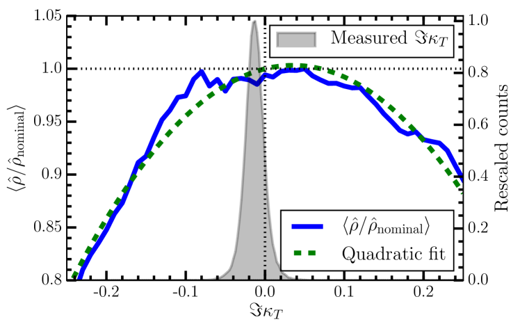
In addition to the dependence of on calibration errors presented in Fig. 9, individual realizations of show an additional variation of approximately due to the power spectral density of the detector noise that is estimated from the strain data. For example, calibration errors affect the estimated noise power spectral density, and as a result, shift the bin boundaries used to calculate the statistic. This subtle shift in the bin boundaries sometimes leads to a deviation in the measured value of of about compared to its value if the bin boundaries had been fixed. The estimate of the noise power spectral density is also affected by the choice of start and end times for the 2048 s segments used to estimate the noise power spectral density, and this also affects for GW150914 by approximately . Overall, since the measured combined re-weighted SNR is significantly above the detection threshold, neglecting the time-variation of the calibration does not affect the result of this search.
Appendix B Analysis of Simulated Signals
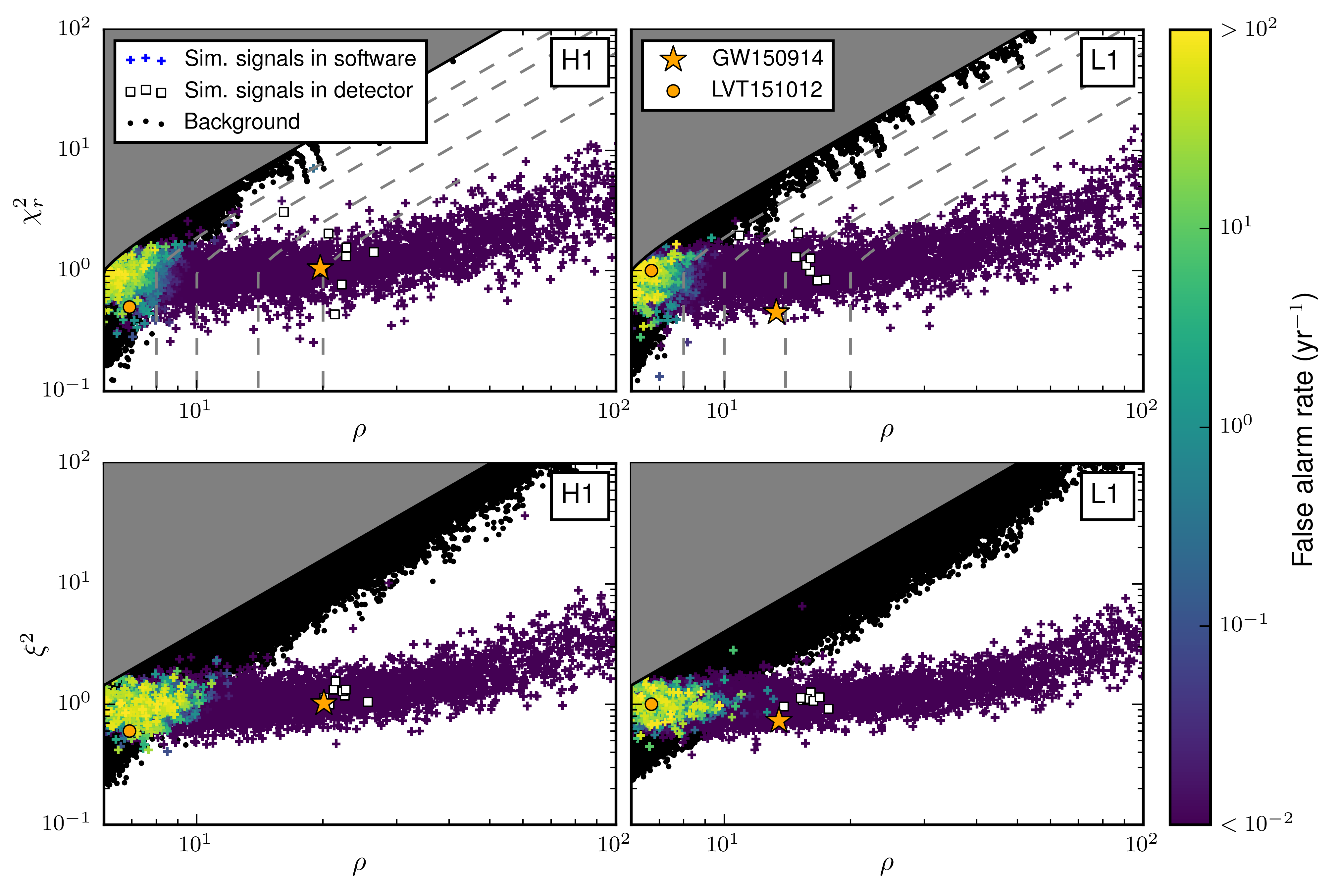
Simulated signals are added to the detector data to validate the performance of our searches. These simulations can be added either in software, by adding a waveform to the input strain data, or by moving the detector’s test masses in a way that simulates a gravitational-wave signal. Physically actuating on the detector’s test masses provides a full end-to-end validation of our ability to detect signals at the expense of corrupting the data during the time of the simulated signal. Adding simulations in software allows us to repeat the analysis on the same data set many times, accumulating large statistics and testing search sensitivity across a large parameter space. Signals simulated in software have been used to constrain the coalescence rate of binary black hole systems in Ref. Abbott et al. (2016g).
To validate the search, we generate a population of binary black holes with component masses between and and the full range of available spins using the template waveform. Signals are randomly distrubted in sky location, orientation, distance, and time, then added coherently to each detector’s strain data prior to filtering. The PyCBC and GstLAL analyses report the matched-filter SNR, and the and statistics, respectively, for these simulated signals. In addition, we simulate eight signals in the detectors to test the recovery of GW150914. The signals were generated using the aligned-spin waveforms used in the search. The parameters were drawn from the posterior distribution of early GW150914 parameter estimation results. The sky position of the signals were chosen to give similar amplitudes as GW150914 in the H1 and L1 detectors Abbott et al. (2016e). The signals are added to both detectors with the correct relative amplitude, phase, and time offsets to simulate a gravitational-wave signal from an astrophysical source.
Figure 10 shows the and versus matched-filter SNR in each detector for a set of software-simulated binary black hole signals recovered by the PyCBC (top) and GstLAL (bottom) analyses. Also shown are the eight simulated signals that were physically added to the detector. The parameters of GW150914 are shown with a star. We see a clear separation between signal and noise background in the region of GW150914 for both the software and physical (hardware) simulations. Simulated gravitational waves with similar parameters and distances as GW150914 are found with high significance by both analyses, validating the ability of the analyses described here to detect sources similar to GW150914.
References
- Abbott et al. (2016a) B. P. Abbott et al. (LIGO Scientific Collaboration, Virgo Collaboration), Phys. Rev. Lett. 116, 061102 (2016a), https://dcc.ligo.org/LIGO-P150914/public/main, arXiv:1602.03847 [gr-qc] .
- Abbott et al. (2016b) B. P. Abbott et al. (LIGO Scientific Collaboration, Virgo Collaboration), (2016b), https://dcc.ligo.org/LIGO-P1500229/public/main, arXiv:1602.03843 [gr-qc] .
- Dal Canton et al. (2014) T. Dal Canton et al., Phys. Rev. D90, 082004 (2014), arXiv:1405.6731 [gr-qc] .
- Usman et al. (2015) S. A. Usman et al., (2015), arXiv:1508.02357.
- Nitz et al. (2016) A. H. Nitz, I. W. Harry, J. L. Willis, C. M. Biwer, D. A. Brown, L. P. Pekowsky, T. Dal Canton, A. R. Williamson, T. Dent, C. D. Capano, T. T. Massinger, A. K. Lenon, A. Nielsen, and M. Cabero, “PyCBC Software,” https://github.com/ligo-cbc/pycbc (2016).
- Cannon et al. (2012) K. Cannon, R. Cariou, A. Chapman, M. Crispin-Ortuzar, N. Fotopoulos, et al., Astrophys.J. 748, 136 (2012), arXiv:1107.2665 [astro-ph.IM] .
- Privitera et al. (2014) S. Privitera, S. R. P. Mohapatra, P. Ajith, K. Cannon, N. Fotopoulos, M. A. Frei, C. Hanna, A. J. Weinstein, and J. T. Whelan, Phys. Rev. D89, 024003 (2014), arXiv:1310.5633 [gr-qc] .
- Messick et al. (2016) C. Messick et al., (2016), arXiv:1604.04324 [astro-ph] .
- Taracchini et al. (2014) A. Taracchini, A. Buonanno, Y. Pan, T. Hinderer, M. Boyle, et al., Phys.Rev. D89, 061502 (2014), arXiv:1311.2544 [gr-qc] .
- Pürrer (2016) M. Pürrer, Phys. Rev. D 93, 064041 (2016), arXiv:1512.02248 .
- Capano et al. (2016) C. Capano, T. Dent, Y.-M. Hu, M. Hendry, C. Messenger, and J. Veitch, (2016), arXiv:1601.00130 [astro-ph.IM] .
- Allen et al. (2012) B. Allen, W. G. Anderson, P. R. Brady, D. A. Brown, and J. D. E. Creighton, Phys.Rev. D85, 122006 (2012), arXiv:gr-qc/0509116 [gr-qc] .
- Cannon et al. (2010a) K. Cannon, A. Chapman, C. Hanna, D. Keppel, A. C. Searle, and A. J. Weinstein, Phys. Rev. D82, 044025 (2010a), arXiv:1005.0012 [gr-qc] .
- Abbott et al. (2016c) B. P. Abbott et al. (LIGO Scientific Collaboration, Virgo Collaboration), (2016c), https://dcc.ligo.org/LIGO-P1500238/public/main, arXiv:1602.03844 [gr-qc] .
- Allen (2005) B. Allen, Phys.Rev. D71, 062001 (2005), arXiv:gr-qc/0405045 [gr-qc] .
- Cannon et al. (2015) K. Cannon, C. Hanna, and J. Peoples, (2015), arXiv:1504.04632 [astro-ph.IM] .
- Abbott et al. (2016d) B. P. Abbott et al. (LIGO Scientific Collaboration, Virgo Collaboration), Phys. Rev. Lett. 116, 131103 (2016a), https://dcc.ligo.org/LIGO-P1500237/public/main, arXiv:1602.03838 [gr-qc] .
- Abbott et al. (2016e) B. P. Abbott et al. (LIGO Scientific Collaboration, Virgo Collaboration), (2016e), https://dcc.ligo.org/LIGO-P1500218/public/main, arXiv:1602.03840 [gr-qc] .
- Gonzalez et al. (2012e) G. Gonzàlez et al. (LIGO Scientific Collaboration, Virgo Collaboration), (2012e), https://dcc.ligo.org/LIGO-M1200055/public/main .
- Thorne (1987) K. S. Thorne, in Three hundred years of gravitation, edited by S. W. Hawking and W. Israel (Cambridge University Press, Cambridge, 1987) Chap. 9, pp. 330–458.
- Sathyaprakash and Dhurandhar (1991) B. S. Sathyaprakash and S. V. Dhurandhar, Phys. Rev. D44, 3819 (1991).
- Cutler et al. (1993) C. Cutler et al., Phys. Rev. Lett. 70, 2984 (1993).
- Finn (1992) L. S. Finn, Phys. Rev. D46, 5236 (1992), arXiv:gr-qc/9209010 [gr-qc] .
- Finn and Chernoff (1993) L. S. Finn and D. F. Chernoff, Phys. Rev. D47, 2198 (1993), arXiv:gr-qc/9301003 [gr-qc] .
- Dhurandhar and Sathyaprakash (1994) S. V. Dhurandhar and B. S. Sathyaprakash, Phys. Rev. D49, 1707 (1994).
- Balasubramanian et al. (1996) R. Balasubramanian, B. S. Sathyaprakash, and S. V. Dhurandhar, Phys. Rev. D 53, 3033 (1996), arXiv:gr-qc/9508011 .
- Flanagan and Hughes (1998) E. E. Flanagan and S. A. Hughes, Phys. Rev. D57, 4535 (1998), arXiv:gr-qc/9701039 [gr-qc] .
- Wainstein and Zubakov (1962) L. A. Wainstein and V. D. Zubakov, Extraction of signals from noise (Prentice-Hall, Englewood Cliffs, NJ, 1962).
- Aasi et al. (2015) J. Aasi et al. (LIGO Scientific), Class.Quant.Grav. 32, 074001 (2015), arXiv:1411.4547 [gr-qc] .
- Abramovici et al. (1992) A. Abramovici et al., Science 256, 325 (1992).
- Abbott et al. (2016f) B. P. Abbott et al. (LIGO Scientific Collaboration), (2016f), https://dcc.ligo.org/LIGO-P1500248/public/main, arXiv:1602.03845 [gr-qc] .
- Peters and Mathews (1963) P. C. Peters and J. Mathews, Phys. Rev. 131, 435 (1963).
- Peters (1964) P. C. Peters, Phys. Rev. 136, B1224 (1964).
- Blanchet et al. (1995) L. Blanchet, T. Damour, B. R. Iyer, C. M. Will, and A. G. Wiseman, Phys. Rev. Lett. 74, 3515 (1995).
- Kidder et al. (1993) L. E. Kidder, C. M. Will, and A. G. Wiseman, Phys. Rev. D47, 4183 (1993), arXiv:gr-qc/9211025 [gr-qc] .
- Kidder (1995) L. E. Kidder, Phys. Rev. D52, 821 (1995), arXiv:gr-qc/9506022 [gr-qc] .
- Blanchet (2014) L. Blanchet, Living Rev. Rel. 17, 2 (2014), arXiv:1310.1528 [gr-qc] .
- Miller and Miller (2014) M. C. Miller and J. M. Miller, Phys.Rept. 548, 1 (2014), arXiv:1408.4145 [astro-ph.HE] .
- Belczynski et al. (2014) K. Belczynski, A. Buonanno, M. Cantiello, C. L. Fryer, D. E. Holz, I. Mandel, M. C. Miller, and M. Walczak, Astrophys. J. 789, 120 (2014), arXiv:1403.0677 [astro-ph.HE] .
- Burgay et al. (2003) M. Burgay et al., Nature. 426, 531 (2003), astro-ph/0312071 .
- Lorimer (2008) D. R. Lorimer, Living Rev. Rel. 11, 8 (2008), arXiv:0811.0762 [astro-ph] .
- McClintock et al. (2013) J. E. McClintock, R. Narayan, and J. F. Steiner, Space Sci. Rev. , 1 (2013), arXiv:1303.1583 [astro-ph.HE] .
- Owen (1996) B. J. Owen, Phys. Rev. D 53, 6749 (1996).
- Owen and Sathyaprakash (1999) B. J. Owen and B. S. Sathyaprakash, Phys. Rev. D 60, 022002 (1999).
- Babak et al. (2006) S. Babak, R. Balasubramanian, D. Churches, T. Cokelaer, and B. S. Sathyaprakash, Class. Quant. Grav. 23, 5477 (2006).
- Cokelaer (2007) T. Cokelaer, Phys. Rev. D76, 102004 (2007), arXiv:0706.4437 [gr-qc] .
- Keppel (2013) D. Keppel, (2013), arXiv:1307.4158 [gr-qc] .
- Harry et al. (2009) I. W. Harry, B. Allen, and B. Sathyaprakash, Phys.Rev. D80, 104014 (2009), arXiv:0908.2090 [gr-qc] .
- Brown et al. (2012) D. A. Brown, I. Harry, A. Lundgren, and A. H. Nitz, Phys.Rev. D86, 084017 (2012), arXiv:1207.6406 [gr-qc] .
- Apostolatos (1996) T. A. Apostolatos, Phys. Rev. D54, 2421 (1996).
- Pan et al. (2014) Y. Pan, A. Buonanno, A. Taracchini, L. E. Kidder, A. H. Mroué, H. P. Pfeiffer, M. A. Scheel, and B. Szilágyi, Phys. Rev. D89, 084006 (2014), arXiv:1307.6232 [gr-qc] .
- Harry et al. (2016) I. Harry, S. Privitera, A. Bohe, and A. Buonanno, (2016), arXiv:1603.02444 [gr-qc] .
- Buonanno et al. (2003) A. Buonanno, Y. Chen, and M. Vallisneri, Phys. Rev. D 67, 104025 (2003), erratum-ibid. 74 (2006) 029904(E).
- Martynov et al. (2016) D. Martynov et al., The Sensitivity of the Advanced LIGO Detectors at the Beginning of Gravitational Wave Astronomy, Tech. Rep. LIGO-P1500260 (LIGO Project, 2016).
- Effler et al. (2015) A. Effler, R. M. S. Schofield, V. V. Frolov, G. Gonzalez, K. Kawabe, J. R. Smith, J. Birch, and R. McCarthy, Class. Quant. Grav. 32, 035017 (2015), arXiv:1409.5160 [astro-ph.IM] .
- Cannon et al. (2010b) K. Cannon, A. Chapman, C. Hanna, D. Keppel, A. C. Searle, and A. J. Weinstein, Phys. Rev. D 82, 044025 (2010b).
- Droz et al. (1999) S. Droz, D. J. Knapp, E. Poisson, and B. J. Owen, Phys. Rev. D 59, 124016 (1999).
- Blanchet et al. (2004) L. Blanchet, T. Damour, G. Esposito-Farèse, and B. R. Iyer, Phys. Rev. Lett. 93, 091101 (2004), gr-qc/0406012 .
- Buonanno and Damour (2000) A. Buonanno and T. Damour, Phys. Rev. D62, 064015 (2000), arXiv:gr-qc/0001013 [gr-qc] .
- Pürrer (2014) M. Pürrer, Class. Quant. Grav. 31, 195010 (2014), arXiv:1402.4146 [gr-qc] .
- Lyons (2008) L. Lyons, Ann. Appl. Stat. 2, 887 (2008).
- Brown et al. (2004) D. A. Brown et al., Class. Quant. Grav. 21, S1625 (2004), arXiv:0705.1572 [gr-qc] .
- Brown (2005) D. A. Brown (LIGO), Class. Quant. Grav. 22, S1097 (2005), gr-qc/0505102 .
- Babak et al. (2013) S. Babak, R. Biswas, P. Brady, D. Brown, K. Cannon, et al., Phys.Rev. D87, 024033 (2013).
- Brown et al. (2006) D. A. Brown et al., in Workflows for e-Science, edited by I. J. Taylor, E. Deelman, D. Gannon, and M. S. Shields (Springer-Verlag, 2006) Chap. 5, pp. 41–61.
- Deelman et al. (2005) E. Deelman, G. Singh, M.-H. Su, J. Blythe, Y. Gil, C. Kesselman, G. Mehta, K. Vahi, G. B. Berriman, J. Good, A. Laity, J. C. Jacob, and D. S. Katz, Scientific Programming Journal 13, 219 (2005).
- Deelman et al. (2015) E. Deelman, K. Vahi, G. Juve, M. Rynge, S. Callaghan, P. J. Maechling, R. Mayani, W. Chen, R. Ferreira da Silva, M. Livny, and K. Wenger, Future Generation Computer Systems 46, 17 (2015), funding Acknowledgements: NSF ACI SDCI 0722019, NSF ACI SI2-SSI 1148515 and NSF OCI-1053575.
- Thain et al. (2005) D. Thain, T. Tannenbaum, and M. Livny, Concurrency - Practice and Experience 17, 323 (2005).
- Couvares et al. (2006) P. Couvares, T. Kosar, A. Roy, J. Weber, and K. Wenger, in Workflows for e-Science, edited by I. J. Taylor, E. Deelman, D. Gannon, and M. S. Shields (Springer-Verlag, 2006) Chap. 22, pp. 357–375.
- Jones et al. (01 ) E. Jones, T. Oliphant, P. Peterson, et al., “SciPy: Open source scientific tools for Python,” (2001–), [Online; accessed 2016-03-28].
- Walt et al. (2011) S. v. d. Walt, S. C. Colbert, and G. Varoquaux, Computing in Science & Engineering 13, 22 (2011).
- Hunter (2007) J. D. Hunter, Computing in Science & Engineering 9, 90 (2007).
- Abbott et al. (2004) B. Abbott et al. (LIGO Scientific), Phys. Rev. D69, 122001 (2004), arXiv:gr-qc/0308069 [gr-qc] .
- Abbott et al. (2005a) B. Abbott et al. (LIGO Scientific), Phys. Rev. D72, 082001 (2005a), arXiv:gr-qc/0505041 [gr-qc] .
- Abbott et al. (2005b) B. Abbott et al. (LIGO Scientific), Phys. Rev. D72, 082002 (2005b), arXiv:gr-qc/0505042 [gr-qc] .
- Abbott et al. (2006) B. Abbott et al. (LIGO Scientific), Phys. Rev. D73, 062001 (2006), arXiv:gr-qc/0509129 [gr-qc] .
- Abbott et al. (2008a) B. Abbott et al. (LIGO Scientific), Phys. Rev. D77, 062002 (2008a), arXiv:0704.3368 [gr-qc] .
- Abbott et al. (2008b) B. Abbott et al. (LIGO Scientific), Phys. Rev. D78, 042002 (2008b), arXiv:0712.2050 [gr-qc] .
- Abbott et al. (2009a) B. Abbott et al. (LIGO Scientific Collaboration), Phys.Rev. D79, 122001 (2009a), arXiv:0901.0302 [gr-qc] .
- Abbott et al. (2009b) B. Abbott et al. (LIGO Scientific Collaboration), Phys. Rev. D 80, 047101 (2009b).
- Abadie et al. (2010) J. Abadie et al. (LIGO Scientific), Phys. Rev. D82, 102001 (2010), arXiv:1005.4655 [gr-qc] .
- Abadie et al. (2012) J. Abadie et al. (LIGO Collaboration, Virgo Collaboration), Phys.Rev. D85, 082002 (2012), arXiv:1111.7314 [gr-qc] .
- Aasi et al. (2013) J. Aasi et al. (LIGO Scientific Collaboration, Virgo Collaboration), Phys.Rev. D87, 022002 (2013), arXiv:1209.6533 [gr-qc] .
- Aasi et al. (2014) J. Aasi et al. (VIRGO, LIGO Scientific), Phys. Rev. D89, 102006 (2014), arXiv:1403.5306 [gr-qc] .
- int (2015) Intel Math Kernel Library (Intel Corporation, 2015).
- Frigo and Johnson (2005) M. Frigo and S. G. Johnson, Proceedings of the IEEE 93, 216 (2005), special issue on “Program Generation, Optimization, and Platform Adaptation”.
- Cutler and Flanagan (1994) C. Cutler and E. Flanagan, Phys. Rev. D 49, 2658 (1994).
- Robinet (2015) F. Robinet, https://tds.ego-gw.it/ql/?c=10651 (2015).
- Babak et al. (2005) S. Babak, H. Grote, M. Hewitson, H. Luck, and K. A. Strain, Phys. Rev. D72, 022002 (2005), arXiv:gr-qc/0502002 [gr-qc] .
- Nitz (2015) A. Nitz, Ph.D. thesis, Syracuse University (2015).
- Skellam (1946) J. G. Skellam, Journal of the Royal Statistical Society 109, 296 (1946).
- Gst (2016) “Gstreamer plugins for the LSC Algorithm Library,” https://www.lsc-group.phys.uwm.edu/daswg/projects/gstlal.html (2016).
- Cannon et al. (2011) K. Cannon, C. Hanna, and D. Keppel, Phys. Rev. D84, 084003 (2011), arXiv:1101.4939 [gr-qc] .
- Cannon (2008) K. C. Cannon, Classical and Quantum Gravity 25, 105024 (2008).
- Silverman (1998) B. W. Silverman, Density Estimation for Statistics and Data Analysis (Chapman & Hall, London, 1998).
- Veitch et al. (2015) J. Veitch, V. Raymond, B. Farr, W. Farr, P. Graff, et al., Phys.Rev. D91, 042003 (2015), arXiv:1409.7215 [gr-qc] .
- Pan et al. (2010) Y. Pan, A. Buonanno, L. T. Buchman, T. Chu, L. E. Kidder, et al., Phys. Rev. D 81, 084041 (2010), arXiv:0912.3466 [gr-qc] .
- Hannam et al. (2014) M. Hannam, P. Schmidt, A. Bohé, L. Haegel, S. Husa, F. Ohme, G. Pratten, and M. Pürrer, Phys. Rev. Lett. 113, 151101 (2014), arXiv:1308.3271 [gr-qc] .
- Khan et al. (2016) S. Khan, S. Husa, M. Hannam, F. Ohme, M. Pürrer, X. J. Forteza, and A. Bohé, Phys. Rev. D93, 044007 (2016), arXiv:1508.07253 [gr-qc] .
- Abbott et al. (2016g) B. P. Abbott et al. (LIGO Scientific Collaboration, Virgo Collaboration), (2016g), https://dcc.ligo.org/LIGO-P1500217/public/main, arXiv:1602.03842 [astro-ph.HE] .
- Abbott et al. (2016h) B. P. Abbott et al. (LIGO Scientific Collaboration, Virgo Collaboration), (2016h), https://dcc.ligo.org/LIGO-P1500213/public/main, arXiv:1602.03841 [gr-qc] .
- Abbott et al. (2016i) B. P. Abbott et al. (LIGO Scientific Collaboration, Virgo Collaboration), Astrophys. J. 818, L22 (2016i), https://dcc.ligo.org/LIGO-P1500262/public/main, arXiv:1602.03846 [astro-ph.HE] .
- Allen (1996) B. Allen, LIGO Calibration Accuracy, Tech. Rep. LIGO-T960189-00-Z (LIGO Project, 1996).
- Brown (for the LIGO Scientific Collaboration) D. A. Brown (for the LIGO Scientific Collaboration), Class. Quantum Grav. 21, S797 (2004).