Interplay between Social Influence and Network Centrality: A Comparative Study on Shapley Centrality and Single-Node-Influence Centrality

Abstract

We study network centrality based on dynamic influence propagation models in social networks. To illustrate our integrated mathematical-algorithmic approach for understanding the fundamental interplay between dynamic influence processes and static network structures, we focus on two basic centrality measures: (a) Single Node Influence (SNI) centrality, which measures each node’s significance by its influence spread; and (b) Shapley Centrality, which uses the Shapley value of the influence spread function — formulated based on a fundamental cooperative-game-theoretical concept — to measure the significance of nodes. We present a comprehensive comparative study of these two centrality measures. Mathematically, we present axiomatic characterizations, which precisely capture the essence of these two centrality measures and their fundamental differences. Algorithmically, we provide scalable algorithms for approximating them for a large family of social-influence instances. Empirically, we demonstrate their similarity and differences in a number of real-world social networks, as well as the efficiency of our scalable algorithms. Our results shed light on their applicability: SNI centrality is suitable for assessing individual influence in isolation while Shapley centrality assesses individuals’ performance in group influence settings.

1 Introduction

Network science is a fast growing discipline that uses mathematical graph structures to represent real-world networks — such as the Web, Internet, social networks, biological networks, and power grids — in order to study fundamental network properties. However, network phenomena are far more complex than what can be captured only by nodes and edges, making it essential to formulate network concepts by incorporating network facets beyond graph structures [36]. For example, network centrality is a key concept in network analysis. The centrality of nodes, usually measured by a real-valued function, reflects their significance, importance, or crucialness within the given network. Numerous centrality measures have been proposed, based on degree, closeness, betweenness and eigenvector (i.e., PageRank) (cf. [23]). However, most of these centrality measures focus only on the static topological structures of the networks, while real-world network data include much richer interaction dynamics beyond static topology.

Influence propagation is a wonderful example of interaction dynamics in social networks. As envisioned by Domingos and Richardson [28, 14], and beautifully formulated by Kempe, Kleinberg, and Tardos [18], social influence propagation can be viewed as a stochastic dynamic process over an underlying static graph: After a group of nodes becomes active, these seed nodes propagate their influence through the graph structure. Even when the static graph structure of a social network is fixed, dynamic phenomena such as the spread of ideas, epidemics, and technological innovations can follow different processes. Thus, network centrality, which aims to measure nodes’ importance in social influence, should be based not only on static graph structure, but also on the dynamic influence propagation process.

In this paper, we address the basic question of how to formulate network centrality measures that reflect dynamic influence propagation. We will focus on the study of the interplay between social influence and network centrality.

A social influence instance specifies a directed graph $G=(V,E)$ and an influence model $P_{{\mathcal{I}}}$ (see Section 2). For each $S\subseteq V$, $P_{{\mathcal{I}}}$ defines a stochastic influence process on $G$ with $S$ as the initial active set, which activates a random set $\boldsymbol{I}(S)\supseteq S$ with probability $P_{{\mathcal{I}}}(S,\boldsymbol{I}(S))$. Then, $\sigma(S)=\mathbb{E}[|\boldsymbol{I}(S)|]$ is the influence spread of $S$. The question above can be restated as: Given a social-influence instance $(V,E,P_{{\mathcal{I}}})$, how should we define the centrality of nodes in $V$?

A natural centrality measure for each node $v\in V$ is its influence spread $\sigma(\{v\})$. However, this measure — referred to as the single node influence (SNI) centrality — completely ignores the influence profile of groups of nodes and a node’s role in such group influence. Thus, other more sensible centrality measures accounting for group influence may better capture nodes’ roles in social influence. As a concrete formulation of group-influence analyses, we apply Shapley value [31] — a fundamental concept from cooperative game theory — to define a new centrality measure for social influence.

Cooperative game theory is a mathematical theory studying people’s performance and behavior in coalitions (cf. [21]). Mathematically, an $n$-person coalitional game is defined by a characteristic function $\tau:2^{V}\rightarrow\mathbb{R}$, where $V=[n]$, and $\tau(S)$ is the utility of the coalition $S$ [31]. In this game, the Shapley value $\phi_{v}^{\textit{Shapley}}(\tau)$ of $v\in V$ is $v$’s expected marginal contribution in a random order. More precisely:

$$\phi_{v}^{\textit{Shapley}}(\tau)=\mathbb{E}_{\boldsymbol{\pi}}[\tau(S_{\boldsymbol{\pi},v}\cup\{v\})-\tau(S_{\boldsymbol{\pi},v})],$$ (1)

where $S_{\boldsymbol{\pi},v}$ denotes the set of players preceding $v$ in a random permutation $\boldsymbol{\pi}$ of $V$: The Shapley value enjoys an axiomatic characterization (see Section 2), and is widely considered to be the fairest measure of a player’s power in a cooperative game.

Utilizing the above framework, we view influence spread $\sigma(\cdot)$ as a characteristic function, and define the Shapley centrality of an influence instance as the Shapley value of $\sigma$.

In this paper, we present a comprehensive comparative study of SNI and Shapley centralities. In the age of Big Data, networks are massive. Thus, an effective solution concept in network science should be both mathematically meaningful and algorithmically efficient. In our study, we will address both the conceptual and algorithmic questions.

Conceptually, influence-based centrality can be viewed as a dimensional reduction from the high dimensional influence model $P_{{\mathcal{I}}}$ to a low dimensional centrality measure. Dimensional reduction of data is a challenging task, because inevitably some information is lost. As highlighted by Arrow’s celebrated impossibility theorem on voting [3], for various (desirable) properties, conforming dimensional reduction scheme may not even exist. Thus, it is fundamental to characterize what each centrality measure captures.

So, “what do Shapley and SNI centralities capture? what are their basic differences?” Axiomatization is an instrumental approach for such characterization. In Section 3, we present our axiomatic characterizations. We present five axioms for Shapley centrality, and prove that it is the unique centrality measure satisfying these axioms. We do the same for the SNI centrality with three axioms. Using our axiomatic characterizations, we then provide a detailed comparison of Shapley and SNI centralities. Our characterizations show that (a) SNI centrality focuses on individual influence and would not be appropriate for models concerning group influence, such as threshold-based models. (b) Shapley centrality focuses on individuals’ “irreplaceable power" in group influence settings, but may not be interpreted well if one prefer to focus on individual influence in isolation.

The computation of influence-based centralities is also a challenging problem: Exact computation of influence spread in the basic independent cascade and linear-threshold models has been shown to be $\#$P-complete [37, 12]. Shapley centrality computation seems to be more challenging since its definition as in Eq. (1) involves $n!$ permutations, and existing Shapley value computation in several simple network games have quadratic or cubic time complexity [19]. Facing these challenges, in Section 4, we present provably-good scalable algorithms for approximating both Shapley and SNI centralities of a large family of social influence instances. Surprisingly, both algorithms share the same algorithm structure, which extends techniques from the recent algorithmic breakthroughs in influence maximization [10, 34, 33]. We further conduct empirical evaluation of Shapley and SNI centralities in a number of real-world networks. Our experiments — see Section 5 — show that our algorithms can scale up to networks with tens of millions of nodes and edges, and these two centralities are similar in several cases but also have noticeable differences.

These combined mathematical/algorithmic/empirical analyses together present (a) a systematic case study of the interplay between influence dynamics and network centrality based on Shapley and SNI centralities; (b) axiomatic characterizations for two basic centralities that precisely capture their similarities and differences; and (c) new scalable algorithms for influence models. We believe that the dual axiomatic-and-algorithmic characterization provides a comparative framework for evaluating other influence-based network concepts in the future.

For presentation clarity, we move the technical proofs into the appendix, which also contains additional technical materials for (algorithmic and axiomatic) generalization to weighted influence models.

1.1 Related Work

Network centrality has been extensively studied (see [23] and the references therein for a comprehensive introduction). Most classical centralities, based on degree, closeness, betweenness, eigenvector, are defined on static graphs. But some also have dynamic interpretations based on random-walks or network flows [8]. Eigenvector centrality [6] and its closely related Katz-[17] and Alpha-centrality [7] can be viewed as some forms of influence measures, since their dynamic processes are non-conservative [15], meaning that items could be replicated and propagated, similar to diffusion of ideas, opinions, etc. PageRank [11, 25] and other random-walk related centralities correspond to conservative processes, and thus may not be suitable for propagation dynamics. Percolation centrality [27] also addresses diffusion process, but its definition only involves static percolation. None of above maps specific propagation models to network centrality. Ghosh et al. [16] maps a linear dynamic process characterized by parameterized Laplacian to centrality but the social influence models we consider in this paper are beyond such linear dynamic framework. Michalak et al. use Shapley value as network centrality [19], but they only consider five basic network games based on local sphere of influence, and their algorithms run in (least) quadratic time. To the best of our knowledge, our study is the first to explicitly map general social network influence propagation models to network centrality.

Influence propagation has been extensively studied, but most focusing on influence maximization tasks [18, 37, 12], which aims to efficiently select a set of nodes with the largest influence spread. The solution is not a centrality measure and the seeds in the solution may not be the high centrality nodes. Borgatti [9] provides clear conceptual discussions on the difference between centralities and such key player set identification problems. Algorithmically, our construction extends the idea of reverse reachable sets, recently introduced in [10, 34, 33] for scalable influence maximization.

In terms of axiomatic characterizations of network centrality, Sabidussi is the first who provides a set of axioms that a centrality measure should satisfy [29]. A number of other studies since then either provide other axioms that a centrality measure should satisfy (e.g. [24, 5, 30]) or a set of axioms that uniquely define a centrality measure (e.g. [2] on PageRank without the damping factor). All of these axiomatic characterizations focus on static graph structures, while our axiomatization focuses on the interplay between dynamic influence processes and static graph structures, and thus our study fundamentally differs from all the above characterizations. While we are heavily influenced by the axiomatic characterization of the Shapley value [31], we are also inspired by social choice theory [3], and particularly by [26] on measures of intellectual influence and [2] on PageRank.

2 Influence and Centrality

In this section, we review the basic concepts about social influence models and Shapley value, and define the Shapley and single node influence centrality measures.

2.1 Social Influence Models

A network-influence instance is usually specified by a triple ${\mathcal{I}}=(V,E,P_{{\mathcal{I}}})$, where a directed graph $G=(V,E)$ represents the structure of a social network, and $P_{{\mathcal{I}}}$ defines the influence model [18]. As an example, consider the classical discrete-time independent cascade (IC) model, in which each directed edge $(u,v)\in E$ has an influence probability $p_{u,v}\in[0,1]$. At time $0$, nodes in a given seed set $S$ are activated while other nodes are inactive. At time $t\geq 1$, for any node $u$ activated at time $t-1$, it has one chance to activate each of its inactive out-neighbor $v$ with an independent probability $p_{u,v}$. When there is no more activation, the stochastic process ends with a random set $\boldsymbol{I}(S)$ of nodes activated during the process. The influence spread of $S$ is $\sigma(S)=\mathbb{E}[|\boldsymbol{I}(S)|]$, the expected number of nodes influenced by $S$. Throughout the paper, we use boldface symbols to represent random variables.

Algorithmically, we will focus on the (random) triggering model [18], which has IC model as a special case. In this model, each $v\in V$ has a random triggering set $\boldsymbol{T}(v)$, drawn from a distribution defined by the influence model over the power set of all in-neighbors of $v$. At time $t=0$, triggering sets $\{\boldsymbol{T}(v)\}_{v\in V}$ are drawn independently, and the seed set $S$ is activated. At $t\geq 1$, if $v$ is not active, it becomes activated if some $u\in\boldsymbol{T}(v)$ is activated at time $t-1$. The influence spread of $S$ is $\sigma(S)=\mathbb{E}[|\boldsymbol{I}(S)|]$, where $\boldsymbol{I}(S)$ denotes the random set activated by $S$. IC is the triggering model that: For each directed edge $(u,v)\in E$, add $u$ to $\boldsymbol{T}(v)$ with an independent probability of $p_{u,v}$. The triggering model can be equivalently viewed under the live-edge graph model: (1) Draw independent random triggering sets $\{\boldsymbol{T}(v)\}_{v\in V}$; (2) form a live-edge graph $\boldsymbol{L}=(V,\{(u,v):u\in\boldsymbol{T}(v)\})$, where $(u,v),u\in\boldsymbol{T}(v)$ is referred as a live edge. For any subgraph $L$ of $G$ and $S\subseteq V$, let $\Gamma(L,S)$ be the set of nodes in $L$ reachable from set $S$. Then set of active nodes with seed set $S$ is $\Gamma(\boldsymbol{L},S)$, and influence spread $\sigma(S)=\mathbb{E}_{\boldsymbol{L}}[|\Gamma(\boldsymbol{L},S)|]=\sum_{L}\Pr(\boldsymbol{L}=L)\cdot|\Gamma(L,S)|$. We say a set function $f(\cdot)$ is monotone if $f(S)\leq f(T)$ whenever $S\subseteq T$, and submodular if $f(S\cup\{v\})-f(S)\geq f(T\cup\{v\})-f(T)$ whenever $S\subseteq T$ and $v\not\in T$. As shown in [18], in any triggering model, $\sigma(\cdot)$ is monotone and submodular, because $|\Gamma(L,S)|$ is monotone and submodular for each graph $L$.

More generally, we define an influence instance as a triple ${\mathcal{I}}=(V,E,P_{{\mathcal{I}}})$, where $G=(V,E)$ represents the underlying network, and $P_{{\mathcal{I}}}:2^{V}\times 2^{V}\rightarrow\mathbb{R}$ defines the probability that in the influence process, any seed set $S\subseteq V$ activates exactly nodes in any target set $T\subseteq V$ and no other nodes: If $\boldsymbol{I}_{{\mathcal{I}}}(S)$ denotes the random set activated by seed set $S$, then $\Pr(\boldsymbol{I}_{{\mathcal{I}}}(S)=T)=P_{{\mathcal{I}}}(S,T)$. This probability profile is commonly defined by a succinct influence model, such as the triggering model, which interacts with network $G$. We also require that: (a) $P_{{\mathcal{I}}}(\emptyset,\emptyset)=1$, $P_{{\mathcal{I}}}(\emptyset,T)=0$, $\forall T\neq\emptyset$, and (b) if $S\not\subseteq T$ then $P_{{\mathcal{I}}}(S,T)=0$, i.e., $S$ always activates itself ($S\subseteq\boldsymbol{I}_{{\mathcal{I}}}(S)$). Such model is also referred to as the progressive influence model. The influence spread of $S$ is:

$$\sigma_{{\mathcal{I}}}(S)=\mathbb{E}[|\boldsymbol{I}_{{\mathcal{I}}}(S)|]=\sum_{T\subseteq V,S\subseteq T}P_{{\mathcal{I}}}(S,T)\cdot|T|.$$

2.2 Coalitional Games and Shapley Values

An $n$-person coalitional game over $V=[n]$ is specified by a characteristic function $\tau:2^{V}\rightarrow\mathbb{R}$, where for any coalition $S\subseteq V$, $\tau(S)$ denotes the cooperative utility of $S$. In cooperative game theory, a ranking function $\phi$ is a mapping from a characteristic function $\tau$ to a vector in $\mathbb{R}^{n}$. A fundamental solution concept of cooperative game theory is the ranking function given by the Shapley value [31]: Let $\Pi$ be the set of all permutations of $V$. For any $v\in V$ and $\pi\in\Pi$, let $S_{\pi,v}$ denote the set of nodes in $V$ preceding $v$ in permutation $\pi$. Then, $\forall v\in V$:

$$\phi^{\textit{Shapley}}_{v}(\tau)= \frac{1}{n!}\sum_{\pi\in\Pi}\left(\tau(S_{\pi,v}\cup\{v\})-\tau(S_{\pi,v})\right)$$

$$= \sum_{S\subseteq V\setminus\{v\}}\frac{|S|!(n-|S|-1)!}{n!}\left(\tau(S\cup\{v\})-\tau(S)\right).$$

We use $\boldsymbol{\pi}\sim\Pi$ to denote that $\boldsymbol{\pi}$ is a random permutation uniformly drawn from $\Pi$. Then:

$$\phi^{\textit{Shapley}}_{v}(\tau)=\mathbb{E}_{\boldsymbol{\pi}\sim\Pi}[\tau(S_{\boldsymbol{\pi},v}\cup\{v\})-\tau(S_{\boldsymbol{\pi},v})].$$ (2)

The Shapley value of $v$ measures $v$’s marginal contribution over the set preceding $v$ in a random permutation.

Shapley [31] proved a remarkable representation theorem: The Shapley value is the unique ranking function that satisfies all the following four conditions: (1) Efficiency: $\sum_{v\in V}\phi_{v}(\tau)=\tau(V)$. (2) Symmetry: For any $u,v\in V$, if $\tau(S\cup\{u\})=\tau(S\cup\{v\})$, $\forall S\subseteq V\setminus\{u,v\}$, then $\phi_{u}(\tau)=\phi_{v}(\tau)$. (3) Linearity: For any two characteristic functions $\tau$ and $\omega$, for any $\alpha,\beta>0$, $\phi(\alpha\tau+\beta\omega)=\alpha\phi(\tau)+\beta\phi(\omega)$. (4) Null Player: For any $v\in V$, if $\tau(S\cup\{v\})-\tau(S)=0$, $\forall S\subseteq V\setminus\{v\}$, then $\phi_{v}(\tau)=0$. Efficiency states that the total utility is fully distributed. Symmetry states that two players’ ranking values should be the same if they have the identical marginal utility profile. Linearity states that the ranking values of the weighted sum of two coalitional games is the same as the weighted sum of their ranking values. Null Player states that a player’s ranking value should be zero if the player has zero marginal utility to every subset.

2.3 Shapley and SNI Centrality

The influence-based centrality measure aims at assigning a value for every node under every influence instance:

Definition 1 (Centrality Measure)

An (influence-based) centrality measure $\psi$ is a mapping from an influence instance ${\mathcal{I}}=(V,E,P_{{\mathcal{I}}})$ to a real vector $(\psi_{v}({\mathcal{I}}))_{v\in V}\in\mathbb{R}^{|V|}$.

The single node influence (SNI) centrality, denoted by $\psi^{\textit{SNI}}_{v}({\mathcal{I}})$, assigns the influence spread of node $v$ as $v$’s centrality measure: $\psi^{\textit{SNI}}_{v}({\mathcal{I}})=\sigma_{{\mathcal{I}}}(\{v\})$.

The Shapley centrality, denoted by $\psi^{\textit{Shapley}}({\mathcal{I}})$, is the Shapley value of the influence spread function $\sigma_{{\mathcal{I}}}$: $\psi^{\textit{Shapley}}({\mathcal{I}})=\phi^{\textit{Shapley}}(\sigma_{{\mathcal{I}}})$. As a subtle point, note that $\phi^{\textit{Shapley}}$ maps from a $2^{|V|}$ dimensional $\tau$ to a $|V|$-dimensional vector, while, formally, $\psi^{\textit{Shapley}}$ maps from $P_{{\mathcal{I}}}$ — whose dimensions is close to $2^{2|V|}$ — to a $|V|$-dimensional vector.

To help understand these definitions, Figure 1 provides a simple example of a $3$-node graph in the IC model with influence probabilities shown on the edges. The associated table shows the result for Shapley and SNI centralities. While SNI is straightforward in this case, the Shapley centrality calculation already looks complex. For example, for node $u$, its second term in the Shapley computation, $\frac{1}{3}(1-p)\cdot 1.5$, accounts for the case where $u$ is ordered in the second place (with probability $1/3$), in which case only when the first-place node (either $v$ or $w$) does not activate $u$ (with probability $1-p$), it could have marginal influence of $1$ in activating itself, and $0.5$ in activating the remaining node. Similarly, the third term for the Shapley computation for node $v$ accounts for the case where $v$ is ordered second and $w$ is ordered first (with probability $1/6$), in which case if $w$ does not activate $u$ (with probability $1-p$), $v$’s marginal influence spread is $1$ for itself and $p$ for activating $u$; while if $w$ activates $u$ (with probability $p$), only when $u$ does not activate $v$ (with probability $0.5$), $v$ has marginal influence of $1$ for itself. The readers can verify the rest. Based on the result, we find that for interval $p\in(1/2,2/3)$, Shapley and SNI centralities do not align in ranking: Shapley places $v,w$ higher than $u$ while SNI puts $u$ higher than $v,w$.

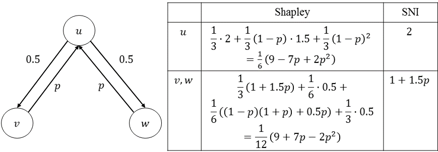
Figure 1: Example on Shapley and SNI centrality.

This simple example already illustrates that (a) computing Shapley centrality could be a nontrivial task; and (b) the relationship between Shapley and SNI centralities could be complicated. Addressing both the computation and characterization questions are the subject of the remaining sections.

3 Axiomatic Characterization

In this section, we present two sets of axioms uniquely characterizing Shapley and SNI centralities, respectively, based on which we analyze their similarities and differences.

3.1 Axioms for Shapley Centrality

Our set of axioms for characterizing the Shapley centrality is adapted from the classical Shapley’s axioms [31].

The first axiom states that labels on the nodes should have no effect on centrality measures. This ubiquitous axiom is similar to the isomorphic axiom in some other centrality characterizations, e.g. [29].

Axiom 1 (Anonymity)

For any influence instance ${\mathcal{I}}=(V,E,P_{{\mathcal{I}}})$, and permutation $\pi\in\Pi$, $\psi_{v}({\mathcal{I}})=\psi_{\pi(v)}({\pi({\mathcal{I}})})$, $\forall v\in V$.

In Axiom 1, $\pi({\mathcal{I}})=(\pi(V),\pi(E),\pi(P_{{\mathcal{I}}}))$ denotes the isomorphic instance: (1) $\forall u,v\in V$, $(\pi(u),\pi(v))\in\pi(E)$ iff $(u,v)\in E$, and (2) $\forall S,T\subseteq V$, $P_{{\mathcal{I}}}(S,T)=P_{\pi({\mathcal{I}})}(\pi(S),\pi(T))$.

The second axiom states that the centrality measure divides the total share of influence $|V|$. In other words, the average centrality is normalized to $1$.

Axiom 2 (Normalization)

For every influence instance ${\mathcal{I}}=(V,E,P_{{\mathcal{I}}})$, $\sum_{v\in V}\psi_{v}({\mathcal{I}})=|V|$.

The next axiom characterizes the centrality of a type of extreme nodes in social influence. In instance ${\mathcal{I}}=(V,E,P_{{\mathcal{I}}})$, we say $v\in V$ is a sink node if $\forall S,T\subseteq V\setminus\{v\}$, $P_{{\mathcal{I}}}(S\cup\{v\},T\cup\{v\})=P_{{\mathcal{I}}}(S,T)+P_{{\mathcal{I}}}(S,T\cup\{v\})$. In the extreme case when $S=T=\emptyset$, $P_{{\mathcal{I}}}(\{v\},\{v\})=1$, i.e., $v$ can only influence itself. When $v$ joins another $S$ to form a seed set, the influence to a target $T\cup\{v\}$ can always be achieved by $S$ alone (except perhaps the influence to $v$ itself). In the triggering model, a sink node is (indeed) a node without outgoing edges, matching the name “sink”.

Because a sink node $v$ has no influence on other nodes, we can “remove” it and obtain a projection of the influence model on the network without $v$: Let ${\mathcal{I}}\setminus\{v\}=(V\setminus\{v\},E\setminus\{v\},P_{{\mathcal{I}}\setminus\{v\}})$ denote the projected instance over $V\setminus\{v\}$, where $E\setminus\{v\}=\{(i,j)\in E:v\not\in\{i,j\}\}$ and $P_{{\mathcal{I}}\setminus\{v\}}$ is the influence model such that for all $S,T\subseteq V\setminus\{v\}$:

$$P_{{\mathcal{I}}\setminus\{v\}}(S,T)=P_{{\mathcal{I}}}(S,T)+P_{{\mathcal{I}}}(S,T\cup\{v\}).$$

Intuitively, since sink node $v$ is removed, the previously distributed influence from $S$ to $T$ and $T\cup\{v\}$ is merged into the influence from $S$ to $T$ in the projected instance. For the triggering model, influence projection is simply removing the sink node $v$ and its incident incoming edges without changing the triggering set distribution of any other nodes.

Axiom 3 below considers the simple case when the influence instance has two sink nodes $u,v\in V$. In such a case, $u$ and $v$ have no influence to each other, and they influence no one else. Thus, their centrality should be fully determined by $V\setminus\{u,v\}$: Removing one sink node — say $v$ — should not affect the centrality measure of another sink node $u$.

Axiom 3 (Independence of Sink Nodes)

For any influence instance ${\mathcal{I}}=(V,E,P_{{\mathcal{I}}})$, for any pair of sink nodes $u,v\in V$ in ${\mathcal{I}}$, it should be the case: $\psi_{u}({\mathcal{I}})=\psi_{u}({{\mathcal{I}}\setminus\{v\}})$.

The next axiom considers Bayesian social influence through a given network: Given a graph $G=(V,E)$, and $r$ influence instances on $G$: ${\mathcal{I}}^{\eta}=(V,E,P_{{\mathcal{I}}^{\eta}})$ with $\eta\in[r]$. Let $\lambda=(\lambda_{1},\lambda_{2},\ldots,\lambda_{r})$ be a prior distribution on $[r]$, i.e. $\sum_{\eta=1}^{r}\lambda_{\eta}=1$, and $\lambda_{\eta}\geq 0$, $\forall\eta\in[r]$. The Bayesian influence instance ${\mathcal{I}}_{\mathcal{B}(\{{\mathcal{I}}^{\eta}\},\lambda)}$ has the following influence process for a seed set $S\subseteq V$: (1) Draw a random index $\boldsymbol{\eta}\in[r]$ according to distribution $\lambda$ (denoted as $\boldsymbol{\eta}\sim\lambda$). (2) Apply the influence process of ${\mathcal{I}}^{\boldsymbol{\eta}}$ with seed set $S$ to obtain the activated set $T$. Equivalently, we have for all $S,T\subseteq V$, $P_{{\mathcal{I}}_{\mathcal{B}(\{{\mathcal{I}}^{\eta}\},\lambda)}}(S,T)=\sum_{\eta=1}^{r}\lambda_{\eta}P_{{\mathcal{I}}^{\eta}}(S,T)$. In the triggering model, we can view each live-edge graph and the deterministic diffusion on it via reachability as an influence instance, and the diffusion of the triggering model is by the Bayesian (or convex) combination of these live-edge instances. The next axiom reflects the linearity-of-expectation principle:

Axiom 4 (Bayesian Influence)

For any network $G=(V,E)$ and Bayesian social-influence model ${\mathcal{I}}_{\mathcal{B}(\{{\mathcal{I}}^{\eta}\},\lambda)}$:

$$\psi_{v}({\mathcal{I}}_{\mathcal{B}(\{{\mathcal{I}}^{\eta}\},\lambda)})=\mathbb{E}_{\boldsymbol{\eta}\sim\lambda}\left[\psi_{v}({\mathcal{I}}^{\boldsymbol{\eta}})\right]=\sum_{\eta=1}^{r}\lambda_{\eta}\cdot\psi_{v}({\mathcal{I}}^{\eta}),\forall v\in V.$$

The above axiom essentially says that the centrality of a Bayesian instance before realizing the actual model ${\mathcal{I}}^{\eta}$ is the same as the expected centrality after realizing ${\mathcal{I}}^{\eta}$.

The last axiom characterizes the centrality of a family of simple social-influence instances. For any $\emptyset\subset R\subseteq U\subseteq V$, a critical set instance ${\mathcal{I}}_{R,U}=(V,E,P_{{\mathcal{I}}_{R,U}})$ is such that: (1) The network $G=(V,E)$ contains a complete directed bipartite sub-graph from $R$ to $U\setminus R$, together with isolated nodes $V\setminus U$. (2) For all $S\supseteq R$, $P_{{\mathcal{I}}_{R,U}}(S,U\cup S)=1$, and (3) For all $S\not\supseteq R$, $P_{{\mathcal{I}}_{R,U}}(S,S)=1$. In ${\mathcal{I}}_{R,U}$, $R$ is called the critical set, and $U$ is called the target set. In other words, a seed set containing $R$ activates all nodes in $U$, but missing any node in $R$ the seed set only activates itself. We use ${\mathcal{I}}_{R,v}$ to denote the special case of $U=R\cup\{v\}$ and $V=U$. That is, only if all nodes in $R$ work together they can activate $v$.

Axiom 5 (Bargaining with Critical Sets)

In any critical set instance ${\mathcal{I}}_{R,v}$, the centrality of $v$ is $\frac{|R|}{|R|+1}$, i.e. $\psi_{v}({\mathcal{I}}_{R,v})=\frac{|R|}{|R|+1}$.

Qualitatively, Axiom 5 together with Normalization and Anonymity axioms implies that the relative importance of $v$ comparing to a node in the critial set $R$ increases when $|R|$ increases, which is reasonable because when the critical set $R$ grows, individuals in $R$ becomes weaker and $v$ becomes relatively stronger. This axiom can be interpreted through Nash’s solution [22] to the bargaining game between a player representing the critical set $R$ and the sink node $v$. Let $r=|R|$. Player $R$ can influence all nodes by itself, achieving utility $r+1$, while player $v$ can only influence itself, with utility $1$. The threat point of this bargaining game is $(r,0)$, which reflects the credits that each player agrees that the other player should at least receive: Player $v$ agrees that player $R$’s contribution is at least $r$, while player $R$ thinks that player $v$ may not have any contribution because $R$ can activate everyone. The slack in this threat point is $\Delta=r+1-(r+0)=1$. However, in this case, player $R$ is actually a coalition of $r$ nodes, and these $r$ nodes have to cooperate in order to influence all $r+1$ nodes — missing any node in $R$ will not influence $v$. The need to cooperative in order to bargain with player $v$ weakens player $R$. The ratio of $v$’s bargaining weight to that of $R$ is thus $1$ to $1/r$. Nash’s bargaining solution [22] provides a fair division of this slack between the two players:

$$(x_{1},x_{2})\in\operatornamewithlimits{argmax}_{x_{1}\geq r,x_{2}\geq 0,x_{1}+x_{2}=r+1}(x_{1}-r)^{1/r}\cdot x_{2}.$$

The unique solution is $(x_{1},x_{2})=(r+\frac{1}{r+1},\frac{r}{r+1})$. Thus, node $v$ should receive a credit of $\frac{r}{r+1}$, as stated in Axiom 5.

Our first axiomatic representation theorem can now be stated as the following:

Theorem 1

(Axiomatic Characterization of Shapley Centrality) The Shapley centrality $\psi^{\textit{Shapley}}$ is the unique centrality measure that satisfies Axioms 1-5. Moreover, every axiom in this set is independent of others.

The soundness of this representation theorem — that the Shapley centrality satisfies all axioms — is relatively simple. However, because of the intrinsic complexity in influence models, the uniqueness proof is in fact complex. We give a high-level proof sketch here and the full proof is in Appendix A.1. We follow Myerson’s proof strategy [21] of Shapley’s theorem. The probabilistic profile $P_{{\mathcal{I}}}$ of influence instance ${\mathcal{I}}=(V,E,P_{{\mathcal{I}}})$ is viewed as a vector in a large space $R^{M}$, where $M$ is the number of independent dimensions in $P_{{\mathcal{I}}}$. Bayesian Influence Axiom enforces that any conforming centrality measure is an affine mapping from $R^{M}$ to $\mathbb{R}^{n}$. We then prove that the critical set instances ${\mathcal{I}}_{R,U}$ form a full-rank basis of the linear space $R^{M}$. Finally, we prove that any axiom-conforming centrality measure over critical set instances (and the additional null instance in which every node is a sink node) must be unique. The uniqueness of the critical set instances and the null instance, the linear independence of critical set instances in $R^{M}$, plus the affine mapping from $R^{M}$ to $\mathbb{R}^{n}$, together imply that the centrality measure of every influence instance is uniquely determined. Our overall proof is more complex and — to a certain degree — more subtle than Myerson’s proof, because our axiomatic framework is based on the influence model in a much larger dimensional space compared to the subset utility functions. Finally, for independence, we need to show that for each axiom, we can construct an alternative centrality measure if the axiom is removed. Except for Axiom 5, the constructions and the proofs for other axioms are nontrivial, and they shed lights on how related centrality measures could be formed when some conditions are relaxed.

3.2 Axioms for SNI Centrality

We first examine which of Axioms 1-5 are satisfied by SNI centrality. It is easy to verify that Anonymity and Bayesian Influence Axioms hold for SNI centrality. For the Independence of Sink Node Axiom (Axiom 3), since every sink node can only influence itself, its SNI centrality is $1$. Thus, Axiom 3 is satisfied by SNI because of a stronger reason.

For the Normalization Axiom (Axiom 2), the sum of single node influence is typically more than the total number of nodes (e.g., when the influence spread is submodular), and thus Axiom 2 does not hold for SNI centrality. The Bargaining with Critical Sets Axiom (Axiom 5) does not hold either, since node $v$ in ${\mathcal{I}}_{R,v}$ is a sink node and thus its SNI centrality is $1$.

We now present our axiomatic characterization of SNI centrality, which will retain Bayesian Influence Axiom 4, strengthen Independence of Sink Node Axiom 3, and recharacterize the centrality of a node in a critical set:

Axiom 6 (Uniform Sink Nodes)

Every sink node has centrality $1$.

Axiom 7 (Critical Nodes)

In any critical set instance ${\mathcal{I}}_{R,U}$, the centrality of a node $w\in R$ is $1$ if $|R|>1$, and is $|U|$ if $|R|=1$.

These three axioms are sufficient to uniquely characterize SNI centrality, as they also imply Anonymity Axiom:

Theorem 2

(Axiomatic Characterization of SNI Centrality) The SNI centrality $\psi^{\textit{SNI}}$ is the unique centrality measure that satisfies Axioms 4, 6, and 7. Moreover, each of these axioms is independent of the others.

Theorems 1 and 2 establish the following appealing property: Even though all our axioms are on probabilistic profiles $P_{{\mathcal{I}}}$ of influence instances, the unique centrality measure satisfying these axioms is in fact fully determined by the influence spread profile $\sigma_{{\mathcal{I}}}$. We find this amazing because the distribution profile $P_{{\mathcal{I}}}$ has much higher dimensionality than its influence-spread profile $\sigma_{{\mathcal{I}}}$.

3.3 Shapley Centrality versus SNI Centrality

We now provide a comparative analysis between Shapley and SNI centralities based on their definitions, axiomatic characterizations, and various other properties they satisfy.

Comparison by definition.  The definition of SNI centrality is more straightforward as it uses individual node’s influence spread as the centrality measure. Shapley centrality is more sophisticatedly formulated, involving groups’ influence spreads. SNI centrality disregards the influence profile of groups. Thus, it may limit its usage in more complex situations where group influences should be considered. Meanwhile, Shapley centrality considers group influence in a particular way involving marginal influence of a node on a given group randomly ordered before the node. Thus, Shapley centrality is more suitable for assessing marginal influence of a node in a group setting.

Comparison by axiomatic characterization.  Both SNI and Shapley centralities satisfy Anonymity, Independence of Sink Nodes, and Bayesian Influence axioms, which seem to be natural axioms for desirable social-influence centrality measures. Their unique axioms characterize exactly their differences. The first difference is on the Normalization Axiom, satisfied by Shapley but not SNI centrality. This indicates that Shapley centrality aims at dividing the total share of possible influence spread $|V|$ among all nodes, but SNI centrality does not enforce such share division among nodes. If we artificially normalize the SNI centrality values of all nodes to satisfy the Normalization Axiom, the normalized SNI centrality would not satisfy the Bayesian Influence Axiom. (In fact, it is not easy to find a new characterization for the normalized SNI centrality similar to Theorem 2.) We will see shortly that the Normalization Axiom would also cause a drastic difference between the two centrality measures for the symmetric IC influence model.

The second difference is on their treatment of sink nodes, exemplified by sink nodes in the critical set instances. For SNI centrality, sink nodes are always treated with the same centrality of $1$ (Axiom 6). But the Shapley centrality of a sink node may be affected by other nodes that influence the sink. In particular, for the critical set instance ${\mathcal{I}}_{R,v}$, $v$ has centrality $|R|/(|R|+1)$, which increases with $R$. As discussed earlier, larger $R$ indicates $v$ is getting stronger comparing to nodes in $R$. In this aspect, Shapley centrality assignment is sensible. Overall, when considering $v$’s centrality, SNI centrality disregards other nodes’ influence to $v$ while Shapley centrality considers other nodes’ influence to $v$.

The third difference is their treatment of critical nodes in the critical set instances. For SNI centrality, in the critical set instance ${\mathcal{I}}_{R,v}$, Axiom 7 obliviously assigns the same value $1$ for nodes $u\in R$ whenever $|R|>1$, effectively equalizing the centrality of node $u\in R$ with $v$. In contrast, Shapley centrality would assign $u\in R$ a value of $1+\frac{1}{|R|(|R|+1)}$, decreasing with $R$ but is always larger than $v$’s centrality of $\frac{|R|}{|R|+1}$. Thus Shapley centrality assigns more sensible values in this case, because $u\in R$ as part of a coalition should have larger centrality than $v$, who has no influence power at all. We believe this shows the limitation of the SNI centrality — it only considers individual influence and disregards group influence. Since the critical set instances reflect the threshold behavior in influence propagation — a node would be influenced only after the number of its influenced neighbors reach certain threshold — this suggests that SNI centrality could be problematic in threshold-based influence models.

Comparison by additional properties.  Finally, we compare additional properties they satisfy. First, it is straightforward to verify that both centrality measures satisfy the Independence of Irrelevant Alternatives (IIA)) property: If an instance ${\mathcal{I}}=(V,E,P_{{\mathcal{I}}})$ is the union of two disjoint and independent influence instances, ${\mathcal{I}}_{1}=(V_{1},E_{1},P_{{\mathcal{I}}_{1}})$ and ${\mathcal{I}}_{2}=(V_{2},E_{2},P_{{\mathcal{I}}_{2}})$, then for $k\in\{1,2\}$ and any $v\in V_{k}$: $\psi_{v}({{\mathcal{I}}})=\psi_{v}({\mathcal{I}}_{k}).$

The IIA property together with the Normalization Axiom leads to a clear difference between SNI and Shapley centrality. Consider an example of two undirected and connected graphs $G_{1}$ with $10$ nodes and $G_{2}$ with $3$ nodes, and the IC model on them with edge probability $1$. Both SNI and Shapley centralities assign same values to nodes within each graph, but due to normalization, Shapley assigns $1$ to all nodes, while SNI assigns $10$ to nodes in $G_{1}$ and $3$ to nodes in $G_{2}$. The IIA property ensures that the centrality does not change when we put $G_{1}$ and $G_{2}$ together. That is, SNI considers nodes in $G_{1}$ more important while Shapley considers them the same. While SNI centrality makes sense from individual influence point of view, the view of Shapley centrality is that a node in $G_{1}$ is easily replaceable by any of the other $9$ nodes in $G_{1}$ but a node in $G_{2}$ is only replaceable by two other nodes in $G_{2}$. Shapley centrality uses marginal influence in randomly ordered groups to determine that the “replaceability factor” cancels out individual influence and assigns same centrality to all nodes.

The above example generalizes to the symmetric IC model where $p_{u,v}=p_{v,u}$, $\forall u,v\in V$: Every node has Shapley centrality of $1$ in such models. The technical reason is that such models have an equivalent undirected live-edge graph representation, containing a number of connected components just like the above example. The Shapley symmetry in the symmetric IC model may sound counter-intuitive, since it appears to be independent of network structures or edge probability values. But we believe what it unveils is that symmetric IC model might be an unrealistic model in practice — it is hard to imagine that between every pair of individuals the influence strength is symmetric. For example, in a star graph, when we perceive that the node in the center has higher centrality, it is not just because of its center position, but also because that it typically exerts higher influence to its neighbors than the reverse direction. This exactly reflects our original motivation that mere positions in a static network may not be an important factor in determining the node centrality, and what important is the effect of individual nodes participating in the dynamic influence process.

From the above discussions, we clearly see that (a) SNI centrality focuses on individual influence in isolation, while (b) Shapley centrality focuses on marginal influence in group influence settings, and measures the irreplaceability of the nodes in some sense.

4 Scalable Algorithms

In this section, we first give a sampling-based algorithm for approximating the Shapley centrality $\psi^{\textit{Shapley}}({\mathcal{I}})$ of any influence instance in the triggering model. We then give a slight adaptation to approximate SNI centrality. In both cases, we characterize the performance of our algorithms and prove that they are scalable for a large family of social-influence instances. In next section, we empirically show that these algorithms are efficient for real-world networks.

4.1 Algorithm for Shapley Centrality

In this subsection, we use $\psi$ as a shorthand for $\psi^{\textit{Shapley}}$. Let $n=|V|$ and $m=|E|$. To precisely state our result, we make the following general computational assumption, as in [34, 33]:

Assumption 1

The time to draw a random triggering set $\boldsymbol{T}(v)$ is proportional to the in-degree of $v$.

The key combinatorial structures that we use are the following random sets generated by the reversed diffusion process of the triggering model. A (random) reverse reachable (RR) set $\boldsymbol{R}$ is generated as follows: (0) Initially, $\boldsymbol{R}=\emptyset$. (1) Select a node $\boldsymbol{v}\sim V$ uniformly at random (called the root of $\boldsymbol{R}$), and add $\boldsymbol{v}$ to $\boldsymbol{R}$. (2) Repeat the following process until every node in $\boldsymbol{R}$ has a triggering set: For every $\boldsymbol{u}\in\boldsymbol{R}$ not yet having a triggering set, draw its random triggering set $\boldsymbol{T}(\boldsymbol{u})$, and add $\boldsymbol{T}(\boldsymbol{u})$ to $\boldsymbol{R}$. Suppose $\boldsymbol{v}\sim V$ is selected in Step (1). The reversed diffusion process uses $\boldsymbol{v}$ as the seed, and follows the incoming edges instead of the outgoing edges to iteratively “influence” triggering sets. Equivalently, an RR set $\boldsymbol{R}$ is the set of nodes in a random live-edge graph $\boldsymbol{L}$ that can reach node $\boldsymbol{v}$.

The following key lemma elegantly connects RR sets with Shapley centrality. We will defer its intuitive explanation to the end of this section. Let $\boldsymbol{\pi}$ be a random permutation on $V$. Let $\mathbb{I}\{{\mathcal{E}}\}$ be the indicator function for event $\mathcal{E}$.

Lemma 1 (Shapley Centrality Identity)

Let $\boldsymbol{R}$ be a random RR set. Then, $\forall u\in V$, $u$’s Shapley centrality is $\psi_{u}=n\cdot\mathbb{E}_{\boldsymbol{R}}[\mathbb{I}\{u\in\boldsymbol{R}\}/|\boldsymbol{R}|]$.

This lemma is instrumental to our scalable algorithm. It guarantees that we can use random RR sets to build unbiased estimators of Shapley centrality. Our algorithm ASV-RR (standing for “Approximate Shapley Value by RR Set”) is presented in Algorithm 1. It takes $\varepsilon$, $\ell$, and $k$ as input parameters, representing the relative error, the confidence of the error, and the number of nodes with top Shapley values that achieve the error bound, respectively. Their exact meaning will be made clear in Theorem 3.

Algorithm 1 ASV-RR$(G,\boldsymbol{T},\varepsilon,\ell,k)$

0:  Network: $G=(V,E)$; Parameters: random triggering set distribution $\{\boldsymbol{T}(v)\}_{v\in V}$, $\varepsilon>0$, $\ell>0$, $k\in[n]$

0:  $\hat{\boldsymbol{\psi}}_{v}$, $\forall v\in V$: estimated centrality measure

1:  {Phase 1. Estimate the number of RR sets needed }

2:  $\boldsymbol{\it LB}=1$; $\varepsilon^{\prime}=\sqrt{2}\cdot\varepsilon$; $\theta_{0}=0$

3:  $\boldsymbol{\it est}_{v}=0$ for every $v\in V$

4:  for $i=1$ to $\lfloor\log_{2}n\rfloor-1$ do

5:     $x=n/2^{i}$

6:     $\theta_{i}=\left\lceil\frac{n\cdot((\ell+1)\ln n+\ln\log_{2}n+\ln 2)\cdot(2+\frac{2}{3}\varepsilon^{\prime})}{\varepsilon^{\prime 2}\cdot x}\right\rceil$

7:     for $j=1$ to $\theta_{i}-\theta_{i-1}$ do

8:        generate a random RR set $\boldsymbol{R}$

9:        for every $\boldsymbol{u}\in\boldsymbol{R}$, $\boldsymbol{\it est}_{\boldsymbol{u}}=\boldsymbol{\it est}_{\boldsymbol{u}}+1/|\boldsymbol{R}|$

10:     end for

11:     $\boldsymbol{\it est}^{(k)}=$ the $k$-th largest value in $\{\boldsymbol{\it est}_{v}\}_{v\in V}$

12:     if  $n\cdot\boldsymbol{\it est}^{(k)}/\theta_{i}\geq(1+\varepsilon^{\prime})\cdot x$ then

13:        $\boldsymbol{\it LB}=n\cdot\boldsymbol{\it est}^{(k)}/(\theta_{i}\cdot(1+\varepsilon^{\prime}))$

14:        break

15:     end if

16:  end for

17:  $\boldsymbol{\theta}=\left\lceil\frac{n((\ell+1)\ln n+\ln 4)(2+\frac{2}{3}\varepsilon)}{\varepsilon^{2}\cdot\boldsymbol{\it LB}}\right\rceil$

18:  {Phase 2. Estimate Shapley value}

19:  $\boldsymbol{\it est}_{v}=0$ for every $v\in V$

20:  for $j=1$ to $\boldsymbol{\theta}$  do

21:     generate a random RR set $\boldsymbol{R}$

22:     for every $\boldsymbol{u}\in\boldsymbol{R}$, $\boldsymbol{\it est}_{\boldsymbol{u}}=\boldsymbol{\it est}_{\boldsymbol{u}}+1/|\boldsymbol{R}|$

23:  end for

24:  for every $v\in V$, $\hat{\boldsymbol{\psi}}_{v}=n\cdot\boldsymbol{\it est}_{v}/\boldsymbol{\theta}$

25:  return $\hat{\boldsymbol{\psi}}_{v}$, $v\in V$

ASV-RR follows the structure of the IMM algorithm of [33] but with some key differences. In Phase 1, Algorithm 1 estimates the number of RR sets needed for the Shapley estimator. For a given parameter $k$, we first estimate a lower bound $\boldsymbol{\it LB}$ of the $k$-th largest Shapley centrality $\psi^{(k)}$. Following a similar structure as the sampling method in IMM [33], the search of the lower bound is carried out in at most $\lfloor\log_{2}n\rfloor-1$ iterations, each of which halves the lower bound target $x=n/2^{i}$ and obtains the number of RR sets $\theta_{i}$ needed in this iteration (line 6). The key difference is that we do not need to store the RR sets and compute a max cover. Instead, for every RR set $\boldsymbol{R}$, we only update the estimate $\boldsymbol{\it est}_{\boldsymbol{u}}$ of each node $\boldsymbol{u}\in\boldsymbol{R}$ with an additional $1/|\boldsymbol{R}|$ (line 9), which is based on Lemma 1. In each iteration, we select the $k$-th largest estimate (line 11) and plug it into the condition in line 12. Once the condition holds, we calculate the lower bound $\boldsymbol{\it LB}$ in line 13 and break the loop. Next we use this $\boldsymbol{\it LB}$ to obtain the number of RR sets $\boldsymbol{\theta}$ needed in Phase 2 (line 17). In Phase 2, we first reset the estimates (line 19), then generate $\boldsymbol{\theta}$ RR sets and again updating $\boldsymbol{\it est}_{u}$ with $1/|\boldsymbol{R}|$ increment for each $\boldsymbol{u}\in\boldsymbol{R}$ (line 22). Finally, these estimates are transformed into the Shapley estimation in line 24.

Unlike IMM, we do not reuse the RR sets generated in Phase 1, because it would make the RR sets dependent and the resulting Shapley centrality estimates biased. Moreover, our entire algorithm does not need to store any RR sets, and thus ASV-RR does not have the memory bottleneck encountered by IMM when dealing with large networks. The following theorem summarizes the performance of Algorithm 1, where $\psi$ and $\psi^{(k)}$ are Shapley centrality and $k$-th largest Shapley centrality value, respectively.

Theorem 3

For any $\epsilon>0$, $\ell>0$, and $k\in[n]$, Algorithm ASV-RR returns an estimated Shapley value $\hat{\boldsymbol{\psi}}_{v}$ that satisfies (a) unbiasedness: $\mathbb{E}[\hat{\boldsymbol{\psi}}_{v}]=\psi_{v},\forall v\in V$; (b) absolute normalization: $\sum_{v\in V}\hat{\boldsymbol{\psi}}_{v}=n$ in every run; and (c) robustness: under the condition that $\psi^{(k)}\geq 1$, with probability at least $1-\frac{1}{n^{\ell}}$:

$$\left\{\begin{array}[]{lr}|\hat{\boldsymbol{\psi}}_{v}-\psi_{v}|\leq\varepsilon\psi_{v}&\forall v\in V\mbox{ with }\psi_{v}>\psi^{(k)},\\ |\hat{\boldsymbol{\psi}}_{v}-\psi_{v}|\leq\varepsilon\psi^{(k)}&\forall v\in V\mbox{ with }\psi_{v}\leq\psi^{(k)}.\end{array}\right.$$ (3)

Under Assumption 1 and the condition $\ell\geq(\log_{2}k-\log_{2}\log_{2}n)/\log_{2}n$, the expected running time of ASV-RR is $O(\ell(m+n)\log n\cdot\mathbb{E}[\sigma(\tilde{\boldsymbol{v}})]/(\psi^{(k)}\varepsilon^{2}))$, where $\mathbb{E}[\sigma(\tilde{\boldsymbol{v}})]$ is the expected influence spread of a random node $\tilde{\boldsymbol{v}}$ drawn from $V$ with probability proportional to the in-degree of $\tilde{\boldsymbol{v}}$.

Eq. (3) above shows that for the top $k$ Shapley values, ASV-RR guarantees the multiplicative error of $\varepsilon$ relative to node’s own Shapley value (with high probability), and for the rest Shapley value, the error is relative to the $k$-th largest Shapley value $\psi^{(k)}$. This is reasonable since typically we only concern nodes with top Shapley values. For time complexity, the condition $\ell\geq(\log_{2}k-\log_{2}\log_{2}n)/\log_{2}n$ always hold if $k\leq\log_{2}n$ or $\ell\geq 1$. When fixing $\varepsilon$ as a constant, the running time depends almost linearly on the graph size ($m+n$) multiplied by a ratio $\mathbb{E}[\sigma(\tilde{\boldsymbol{v}})]/\psi^{(k)}$. This ratio is upper bounded by the ratio between the largest single node influence and the $k$-th largest Shapley value. When these two quantities are about the same order, we have a near-linear time, i.e., scalable [35], algorithm. Our experiments show that in most datasets tested the ratio $\mathbb{E}[\sigma(\tilde{\boldsymbol{v}})]/\psi^{(k)}$ is indeed less than $1$. Moreover, if we could relax the robustness requirement in Eq. (3) to allow the error of $|\hat{\boldsymbol{\psi}}_{v}-\psi_{v}|$ to be relative to the largest single node influence, then we could indeed slightly modify the algorithm to obtain a near-linear-time algorithm without the ratio $\mathbb{E}[\sigma(\tilde{\boldsymbol{v}})]/\psi^{(k)}$ in the time complexity (see Appendix C.5).

The accuracy of ASV-RR is based on Lemma 1 while the time complexity analysis follows a similar structure as in [33]. The proofs of Lemma 1 and Theorem 3 are presented in Appendix C. Here, we give a high-level explanation. In the triggering model, as for influence maximization [10, 34, 33], a random RR set $\boldsymbol{R}$ can be equivalently obtained by first generating a random live-edge graph $\boldsymbol{L}$, and then constructing $\boldsymbol{R}$ as the set of nodes that can reach a random $\boldsymbol{v}\sim V$ in $\boldsymbol{L}$. The fundamental equation associated with this live-edge graph process is:

$$\sigma(S)=\sum_{L}\Pr_{\boldsymbol{L}}(\boldsymbol{L}=L)\Pr_{\boldsymbol{v}}(\boldsymbol{v}\in\Gamma(L,S))\cdot n.$$ (4)

Our Lemma 1 is the result of the following crucial observations: First, the Shapley centrality $\psi_{u}$ of node $u\in V$ can be equivalently formulated as the expected Shapley centrality of $u$ over all live-edge graphs and random choices of root $\boldsymbol{v}$, from Eq. (4). The chief advantage of this formulation is that it localizes the contribution of marginal influences: On a fixed live-graph $L$ and root $v\in V$, we only need to compute the marginal influence of $u$ in terms of activating $v$ to obtain the Shapley contribution of the pair. We do not need to compute the marginal influences of $u$ for activating other nodes. Lemma 1 then follows from our second crucial observation. When $R$ is the fixed set that can reach $v$ in $L$, the marginal influence of $u$ activating $v$ in a random order is $1$ if and only if the following two conditions hold concurrently: (a) $u$ is in $R$ — so $u$ has chance to activate $v$, and (b) $u$ is ordered before any other node in $R$ — so $u$ can activate $v$ before other nodes in $R$ do so. In addition, in a random permutation $\boldsymbol{\pi}\sim\Pi$ over $V$, the probability that $u\in R$ is ordered first in $R$ is exactly $1/|R|$. This explains the contribution of $\mathbb{I}\{u\in\boldsymbol{R}\}/|\boldsymbol{R}|$ in Lemma 1, which is also precisely what the updates in lines 9 and 22 of Algorithm 1 do. The above two observations together establish Lemma 1, which is the basis for the unbiased estimator of $u$’s Shapley centrality. Then, by a careful probabilistic analysis, we can bound the number of random RR sets needed to achieve approximation accuracy stated in Theorem 3 and establish the scalability for Algorithm ASV-RR.

4.2 Algorithm for SNI Centrality

Algorithm 1 relies on the key fact given in Lemma 1 about the Shapley centrality: $\psi^{\textit{Shapley}}_{u}=n\cdot\mathbb{E}_{\boldsymbol{R}}[\mathbb{I}\{u\in\boldsymbol{R}\}/|\boldsymbol{R}|]$. A similar fact holds for the SNI centrality: $\psi^{\textit{SNI}}_{u}=\sigma(\{u\})=n\cdot\mathbb{E}_{\boldsymbol{R}}[\mathbb{I}\{u\in\boldsymbol{R}\}]$ [10, 34, 33]. Therefore, it is not difficult to verify that we only need to replace $\boldsymbol{\it est}_{\boldsymbol{u}}=\boldsymbol{\it est}_{\boldsymbol{u}}+1/|\boldsymbol{R}|$ in lines 9 and 22 with $\boldsymbol{\it est}_{\boldsymbol{u}}=\boldsymbol{\it est}_{\boldsymbol{u}}+1$ to obtain an approximation algorithm for SNI centrality. Let ASNI-RR denote the algorithm adapted from ASV-RR with the above change, and let $\psi_{v}$ below denote SNI centrality $\psi^{\textit{SNI}}_{v}$ and $\psi^{(k)}$ denote the $k$-th largest SNI value.

Theorem 4

For any $\epsilon>0$, $\ell>0$, and $k\in\{1,2,\ldots,n\}$, Algorithm ASNI-RR returns an estimated SNI centrality $\hat{\boldsymbol{\psi}}_{v}$ that satisfies (a) unbiasedness: $\mathbb{E}[\hat{\boldsymbol{\psi}}_{v}]=\psi_{v},\forall v\in V$; and (b) robustness: with probability at least $1-\frac{1}{n^{\ell}}$:

$$\left\{\begin{array}[]{lr}|\hat{\boldsymbol{\psi}}_{v}-\psi_{v}|\leq\varepsilon\psi_{v}&\forall v\in V\mbox{ with }\psi_{v}>\psi^{(k)},\\ |\hat{\boldsymbol{\psi}}_{v}-\psi_{v}|\leq\varepsilon\psi^{(k)}&\forall v\in V\mbox{ with }\psi_{v}\leq\psi^{(k)}.\end{array}\right.$$ (5)

Under Assumption 1 and the condition $\ell\geq(\log_{2}k-\log_{2}\log_{2}n)/\log_{2}n$, the expected running time of ASNI-RR is $O(\ell(m+n)\log n\cdot\mathbb{E}[\sigma(\tilde{\boldsymbol{v}})]/(\psi^{(k)}\varepsilon^{2}))$, where $\mathbb{E}[\sigma(\tilde{\boldsymbol{v}})]$ is the same as defined in Theorem 1.

Together with Algorithm ASV-RR and Theorem 3, we see that although Shapley and SNI centrality are quite different conceptually, surprisingly they share the same RR-set based scalable computation structure. Comparing Theorem 4 with Theorem 3, we can see that computing SNI centrality should be faster for small $k$ since the $k$-th largest SNI value is usually larger than the $k$-th largest Shapley value.

5 Experiments

We conduct experiments on a number of real-world social networks to compare their Shapley and SNI centrality, and test the efficiency of our algorithms ASV-RR and ASNI-RR.

5.1 Experiment Setup

Table 1: Datasets used in the experiments. “# Edges” refers to the number of undirected edges for the first three datasets and the number of directed edges for the last dataset.

Dataset	# Nodes	# Edges	Weight Setting
Data mining (DM)	679	1687	WC, PR, LN
Flixster (FX)	29,357	212,614	LN
DBLP (DB)	654,628	1,990,159	WC, PR
LiveJournal (LJ)	4,847,571	68,993,773	WC

The network datasets we used are summarized in Table 1.

The first dataset is a relatively small one used as a case study. It is a collaboration network in the field of Data Mining (DM), extracted from the ArnetMiner archive (arnetminer.org) [32]: each node is an author and two authors are connected if they have coauthored a paper. The mapping from node ids to author names is available, allowing us to gain some intuitive observations of the centrality measure. We use three large networks to demonstrate the effectiveness of the Shapley and SNI centrality and the scalability of our algorithms. Flixster (FX) [4] is a directed network extracted from movie rating site flixster.com. The nodes are users and a directed edge from $u$ to $v$ means that $v$ has rated some movie(s) that $u$ rated earlier. Both network and the influence probability profile are obtained from the authors of [4], which shows how to learn topic-aware influence probabilities. We use influence probabilities on topic 1 in their provided data as an example. DBLP (DB) is another academic collaboration network extracted from online archive DBLP (dblp.uni-trier.de) and used for influence studies in [37]. Finally, LiveJournal (LJ) is the largest network we tested with. It is a directed network of bloggers, obtained from Stanford’s SNAP project [1], and it was also used in [34, 33].

Table 2: Top 10 authors from DM dataset, ranked by Shapley, SNI, and degree centrality.

We use the independent cascade (IC) model in our experiments. The schemes for generating influence-probability profiles are also shown in Table 1, where WC, PR, and LN stand for weighted cascade, PageRank-based, and learned from real data, respectively. WC is a scheme of [18], which assigns $p_{u,v}=1/d_{v}$ to edge $(u,v)\in E$, where $d_{v}$ is the in-degree of node $v$. PR uses the nodes’ PageRanks [11] instead of in-degrees: We first compute the PageRank score $r(v)$ for every node $v\in V$ in the unweighted network, using $0.15$ as the restart parameter. Note that in our influence network, edge $(u,v)$ means $u$ has influence to $v$; then when computing PageRank, we should reverse the edge direction to $(v,u)$ so that $v$ gives its PageRank vote to $u$, in order to be consistent on influence direction. Then, for each original edge $(u,v)\in E$, PR assigns an edge probability of $r(u)/(r(u)+r(v))\cdot n/(2m^{U})$, where $m^{U}$ is the number of undirected edges in the graph. The assignment achieves the effect that a higher PageRank node has larger influence to a lower PageRank nodes than the reverse direction (when both directions exist). The scaling factor $n/(2m^{U})$ is to normalize the total edge probabilities to $\Theta(n)$, which is similar to the setting of WC. PR defines a PageRank-based asymmetric IC model. LN applies to DM and FX datasets, where we obtain learned influence probability profiles from the authors of the original studies. For the DM dataset, the influence probabilities on edges are learned by the topic affinity algorithm TAP proposed in [32]; for FX, the influence probabilities are learned using maximum likelihood from the action trace data of user rating events.

We implement all algorithms in Visual C++, compiled in Visual Studio 2013, and run our tests on a server computer with 2.4GHz Intel(R) Xeon(R) E5530 CPU, 2 processors (16 cores), 48G memory, and Windows Server 2008 R2 (64 bits).

5.2 Experiment Results

Case Study on DM.  We set $\varepsilon=0.01$, $\ell=1$, and $k=50$ for both ASV-RR and and ASNI-RR algorithms. For the three influence profiles: WC, PR, and LN, Table 2 lists the top 10 nodes in both Shapley and SNI ranking together with their numerical values. The names appeared in all ranking results are well-known data mining researchers in the field, at the time of the data collection 2009, but the ranking details have some difference.

We compare the Shapley ranking versus SNI ranking under the same probability profiles. In general, the two top-10 ranking results align quite well with each other, showing that in these influence instances, high individual influence usually translates into high marginal influence. Some noticeable exception also exists. For example, Christos Faloutsos is ranked No.3 in the DM-PR Shapley centrality, but he is not in Top-10 based on DM-PR individual influence ranking. Conceptually, this would mean that, in the DM-PR model, Professor Faloutsos has better Shapley ranking because he has more unique and marginal impact comparing to his individual influence. In terms of the numerical values, SNI values are larger than the Shapley values, which is expected due to the normalization factor in Shapley centrality.

We next compare Shapley and SNI centrality with the structure-based degree centrality. The results show that the Shapley and SNI rankings in DM-WC and DM-PR are similar to the degree centrality ranking, which is reasonable because DM-WC and DM-PR are all heavily derived from node degrees. However, DM-LN differs from degree ranking a lot, since it is derived from topic modeling, not node degrees. This implies that when the influence model parameters are learned from real-world data, it may contain further information such that its influence-based Shapley or SNI ranking may differ from structure-based ranking significantly.

When comparing the numerical values of the same centrality measure but across different influence models, we see that Shapley values of top researchers in DM-LN are much higher than Shapley values of top researchers under DM-WC or DM-PR, which suggests that influence models learned from topic profiles differentiating nodes more than the synthetic WC or PR methods.

The above results differentiating DM-LN from DM-WC and DM-PR clearly demonstrate the interplay between social influence and network centrality: Different influence processes can lead to different centrality rankings, but when they share some aspects of common “ground-truth” influence, their induced rankings are more closely correlated.

Tuning Parameter $\varepsilon$

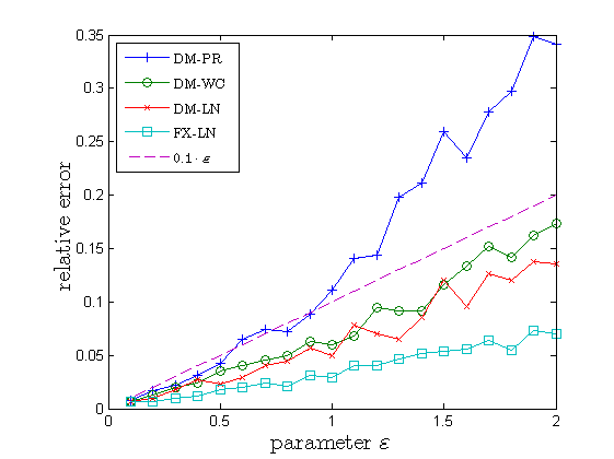
(a) Shapley computation

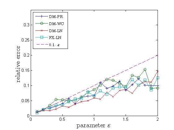
(b) SNI computation

Figure 2: Relative error of centrality computation when $\varepsilon$ setting increases.

We now investigate the impact of our ASV-RR/ASNI-RR parameters, to be applied to our tests on large datasets. Parameter $\ell$ is a simple parameter controlling the probability, $1-\frac{1}{n^{\ell}}$, that the accuracy guarantee holds. We set it to $1$, which is the same as in [34, 33]. For parameter $\varepsilon$, a smaller value improves accuracy at the cost of higher running time. Thus, we want to set $\varepsilon$ at a proper level to balance accuracy and efficiency.

We test different $\varepsilon$ values from $0.1$ to $2$, on both DM and FX datasets, for both algorithms. To evaluate the accuracy, we use the results from $\varepsilon^{*}=0.01$ as the benchmark: For $v\in V$, suppose $s^{*}_{v}$ and $s_{v}$ are the Shapley values computed for $\varepsilon^{*}=0.01$ and a larger $\varepsilon$ value, respectively. Then, we compute $|s_{v}-s^{*}_{v}|/s^{*}_{v}$ and use it as the relative error at $v$. Since the top rankers’ relative errors are more important, we take top 50 nodes from the two ranking results (using $\varepsilon^{*}$ and $\varepsilon$ respectively), and compute the average relative error over the union of these two sets of top 50 nodes. Accordingly, we set parameter $k=50$. We also apply the same relative error computation to SNI centrality.

Figure 2 reports our results on the three DM options and the FX dataset, for both Shapley and SNI computations. We can see clearly that when $\varepsilon\leq 0.5$, the relative errors of all datasets are within $0.05$. In general, the actual relative error is below one tenth of $\varepsilon$ in most cases, except for DM-PR dataset with $\varepsilon\geq 1$. Hence, for the tests on large datasets, we use $\varepsilon=0.5$ to provide reasonable accuracy for top values. Comparing to $\varepsilon=0.01$, this reduces the running time $2500$ fold, because the running time is proportional to $1/\varepsilon^{2}$.

Results on Large Networks.  We conduct experiments to evaluate both the effectiveness and the efficiency of our ASV-RR algorithm on large networks. For large networks, it is no longer easy to inspect rankings manually, especially when these datasets lack user profiles. For the effectiveness, we assess the effectiveness of Shapley and SNI centrality rankings through the lens of influence maximization. In particular, we use top rankers of Shapley/SNI centrality as seeds and measure their effectiveness for influence maximization. We compare the quality and performance of our algorithm with the state-of-the-art scalable algorithm IMM proposed in [33] for influence maximization. Note that the IMM algorithm is based on the RR set approach. For IMM, we set its parameters as $\varepsilon=0.5$, $\ell=1$, and $k=50$, matching the parameter settings we use for ASV-RR/ASNI-RR. We also choose a baseline algorithm Degree, which is based on degree centrality to select top degree nodes as seeds for influence maximization.

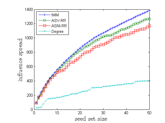
(a) Flixster-LN

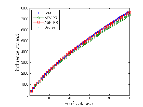
(b) DBLP-WC

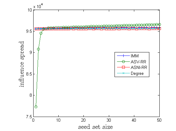
(c) DBLP-PR

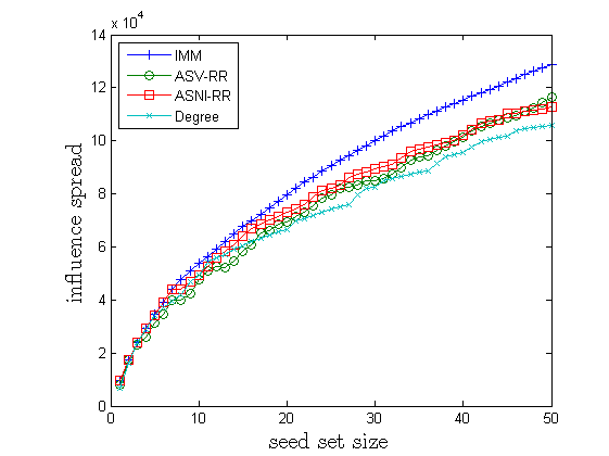
(d) LiveJournal-WC

Figure 3: Influence maximization test on IMM, ASV-RR, and Degree.

We run ASV-RR, ASNI-RR, IMM, and Degree on four influence instances: (1) the Flixster network with learned probability, (2) the DBLP network with WC parameters, (3) the DBLP network with PR parameters, and (4) the LiveJournal network with WC parameters. Figure 3 shows the results of these four tests whose objectives are to identify 50 influential seed nodes. The influence spread in each case is obtained by running 10K Monte Carlo simulations and taking the average value. The results on all datasets in general show that both Shapley and SNI centrality performs reasonably well for the influence maximization task, but in some cases IMM is still noticeably better. This is because IMM is specially designed for the influence maximization task while Shapley and SNI are two centrality measures related to influence but not specialized for the influence maximization task. For the FX-LN dataset, Shapley top rankers performs noticeably better than SNI top rankers (average $8.3\%$ improvement). This is perhaps due to that Shapley centrality accounts for more marginal influence, which is closer to what is needed for influence maximization. This is also the test where they both significantly outperform the baseline Degree heuristic, again indicating that influence learned from the real-world data may contain significantly more information than the graph structure, in which case degree centrality is not a good index for node importance.

The behavior of DBLP-PR needs a bit more attention. For ASNI-RR (as well as IMM and Degree), the first seed selected already generates influence spread of $95K$, but subsequent seeds only have very small marginal contribution to the influence spread. On the contrary, the first seed selected by ASV-RR only has influence spread of $77K$, and the spread reaches the level of ASNI-RR at the fourth seed. Looking more closely, the first seed selected by ASV-RR has Shapley centrality of $10.3$ but its influence spread of $77K$ is only ranked at around $68K$ on SNI ranking, while the first seed of ASNI-RR has Shapley centrality of $3.15$, with Shapley ranking beyond $2100$. This shows that when a large portion of nodes have high individual but overlapping influence (due to the emergence of the giant component in live-edge graphs), they all become more or less replaceable, and thus Shapley ranking, which focuses on marginal influence in a random order, would differs from SNI ranking significantly.

Finally, we evaluate the scalability of ASV-RR and ASNI-RR, and use IMM as a reference point, even though IMM is designed for a different task. We use the same setting of $\varepsilon=0.5$, $\ell=1$, and $k=50$. Table 3 reports the running time of the three algorithms on four large influence instances. For FX-LN, DB-WC, and LJ-WC, the general trend is that IMM is the fastest, followed by ASNI-RR, and then ASV-RR. This is expected, because the theoretical running time of IMM is $\Theta((k+\ell)(m+n)\log n\cdot\mathbb{E}[\sigma(\tilde{\boldsymbol{v}})]/(OPT_{k}\cdot\varepsilon^{2}))$, where $OPT_{k}$ is maximum influence spread with $k$ seeds. Thus comparing to the running time results in Theorems 3 and 4, typically $OPT_{k}$ is much larger than the $k$-th largest SNI centrality, which in turn is much larger than the $k$-th largest Shapley centrality, which leads to the observed running time result. Nevertheless, both ASNI-RR and ASV-RR could be considered efficient in these cases and they can scale to large graphs with tens of millions of nodes and edges.

DB-PR again is an out-lier, with ASNI-RR faster than IMM, and ASV-RR being too slow and inefficient. This is because a large portion of nodes have large individual but overlapping influence, so that $OPT_{50}=95.9K$ is almost the same as the $50$-th largest SNI value ($94.2K$), in which case the $(k+\ell)$ factor in the running time of IMM dominates and makes IMM slower than ASNI-RR. As for ASV-RR, due to the severe overlapping influence, the $50$-th largest Shapley value ($5.10$) is much smaller than the $50$-th largest SNI value or $OPT_{50}$, resulting in much slower running time for ASV-RR.

Table 3: Running time (in seconds).

Algorithm	FX-LN	DB-WC	DB-PR	LJ-WC
ASV-RR	24.83	838.27	594752	8295.57
ASNI-RR	1.36	61.41	28.42	267.50
IMM	0.62	18.08	336.63	54.88

In summary, our experimental results on small and large datasets demonstrate that (a) Shapley and SNI centrality behaves similarly in these networks, but with noticeable differences; (b) for the influence maximization task, they perform close to the specially designed IM algorithm, with Shapley centrality noticeably better than SNI in some case; and (c) both can scale to large graphs with tens of millions of edges, with ASNI-RR having better scalability. except that ASV-RR would not be efficient for graphs with a huge gap between individual influence and marginal influence. Finally, we remark that ASV-RR and ASNI-RR do not need to store RR sets, which eliminates a memory bottleneck that could be encountered by IMM on large datasets.

6 Conclusion and Future Work

Through an integrated mathematical, algorithmic, and empirical study of Shapley and SNI centralities in the context of network influence, we have shown that (a) both enjoy concise axiomatic characterizations, which precisely capture their similarity and differences; (b) both centrality measures can be efficiently approximated with guarantees under the same algorithmic structure, for a large class of influence models; and (c) Shapley centrality focuses on nodes’ marginal influence and their irreplaceability in group influence settings, while SNI centrality focuses on individual influence in isolation, and is not suitable in assessing nodes’ ability in group influence setting, such as threshold-based models.

There are several directions to extend this work and further explore the interplay between social influence and network centrality. One important direction is to formulate centrality measures that combine the advantages of Shapley and SNI centralities, by viewing Shapley and SNI centralities as two extremes in a centrality spectrum, one focusing on individual influence while the other focusing on marginal influence in groups of all sizes. Then, would there be some intermediate centrality measure that provides a better balance? Another direction is to incorporate other classical centralities into influence-based centralities. For example, SNI centrality may be viewed as a generalized version of degree centrality, because when we restrict the influence model to deterministic activation of only immediate neighbors, SNI centrality essentially becomes degree centrality. What about the general forms of closeness, betweenness, PageRank in the influence model? Algorithmically, efficient algorithms for other influence models such as general threshold models [18] is also interesting. In summary, this paper lays a foundation for the further development of the axiomatic and algorithmic theory for influence-based network centralities, which we hope will provide us with deeper insights into network structures and influence dynamics.

Appendix A Proofs on Axiomatic Characterization

A.1 Proof of Theorem 1

We use $\mathcal{A}$ to denote the set of Axioms 1-5.

Analysis of Sink Nodes

We first prove that the involvement of sink nodes in the influence process is what we have expected: (1) The marginal contribution of a sink node $v$ is equal to the probability that $v$ is not influenced by the seed set. (2) For any other node $u\in V$, $u$’s activation probability is the same whether or not $v$ is in the seed set.

Lemma 2

Suppose $v$ is a sink node in ${\mathcal{I}}=(V,E,P_{{\mathcal{I}}})$. Then, (a) for any $S\subseteq V\setminus\{v\}$:

$$\sigma_{\mathcal{I}}(S\cup\{v\})-\sigma_{\mathcal{I}}(S)=\Pr(v\not\in\boldsymbol{I}_{\mathcal{I}}(S)).$$

(b) for any $u\neq v$ and any $S\subseteq V\setminus\{u,v\}$:

$$\Pr(u\not\in\boldsymbol{I}_{\mathcal{I}}(S\cup\{v\}))=\Pr(u\not\in\boldsymbol{I}_{\mathcal{I}}(S)).$$

Proof A.5.

For (a), by the definitions of $\sigma_{\mathcal{I}}$ and sink nodes:

$$\sigma_{\mathcal{I}}(S\cup\{v\})$$

$$=\sum_{T\supseteq S\cup\{v\}}P_{{\mathcal{I}}}(S\cup\{v\},T)\cdot|T|$$

$$=\sum_{T\supseteq S\cup\{v\}}\left(P_{{\mathcal{I}}}(S,T\setminus\{v\})+P_{{\mathcal{I}}}(S,T)\right)\cdot|T|$$

$$=\sum_{T\supseteq S,T\subseteq V\setminus\{v\}}P_{{\mathcal{I}}}(S,T)(|T|+1)+\sum_{T\supseteq S\cup\{v\}}P_{{\mathcal{I}}}(S,T)\cdot|T|$$

$$=\sum_{T\supseteq S}P_{{\mathcal{I}}}(S,T)\cdot|T|+\sum_{T\supseteq S,T\subseteq V\setminus\{v\}}P_{{\mathcal{I}}}(S,T)$$

$$=\sigma_{\mathcal{I}}(S)+\Pr(v\not\in\boldsymbol{I}_{\mathcal{I}}(S)).$$

For (b),

$$\Pr(u\not\in\boldsymbol{I}_{\mathcal{I}}(S\cup\{v\}))$$

$$=\sum_{T\supseteq S\cup\{v\},T\subseteq V\setminus\{u\}}P_{{\mathcal{I}}}(S\cup\{v\},T)$$

$$=\sum_{T\supseteq S\cup\{v\},T\subseteq V\setminus\{u\}}\left(P_{{\mathcal{I}}}(S,T\setminus\{v\})+P_{{\mathcal{I}}}(S,T)\right)$$

$$=\sum_{T\supseteq S,T\subseteq V\setminus\{u\}}P_{{\mathcal{I}}}(S,T)=\Pr(u\not\in\boldsymbol{I}_{\mathcal{I}}(S)).$$

Lemma 2 immediately implies that for any two sink nodes $u$ and $v$, $u$’s marginal contribution to any $S\subseteq V\setminus\{u,v\}$ is the same as its marginal contribution to $S\cup\{v\}$:

Lemma A.6 (Independence between Sink Nodes).

If $u$ and $v$ are two sink nodes in ${\mathcal{I}}$, then for any $S\subseteq V\setminus\{u,v\}$, $\sigma_{\mathcal{I}}(S\cup\{v,u\})-\sigma_{\mathcal{I}}(S\cup\{v\})=\sigma_{\mathcal{I}}(S\cup\{u\})-\sigma_{\mathcal{I}}(S)$.

Proof A.7.

By Lemma 2 (a) and (b), both sides are equal to $\Pr(u\not\in\boldsymbol{I}_{\mathcal{I}}(S))$.

The next two lemmas connect the influence spreads in the original and projected instances.

Lemma A.8.

If $v$ is a sink in ${\mathcal{I}}$, then for any $S\subseteq V\setminus\{v\}$:

$$\sigma_{{\mathcal{I}}\setminus\{v\}}(S)=\sigma_{\mathcal{I}}(S)-\Pr(v\in\boldsymbol{I}_{\mathcal{I}}(S)).$$

Proof A.9.

By the definition of influence projection:

$$\sigma_{{\mathcal{I}}\setminus\{v\}}(S)$$

$$=\sum_{T\supseteq S,T\subseteq V\setminus\{v\}}P_{{\mathcal{I}}\setminus\{v\}}(S,T)\cdot|T|$$

$$=\sum_{T\supseteq S,T\subseteq V\setminus\{v\}}\left(P_{{\mathcal{I}}}(S,T)+P_{{\mathcal{I}}}(S,T\cup\{v\})\right)\cdot|T|$$

$$=\sum_{T\supseteq S,T\subseteq V\setminus\{v\}}P_{{\mathcal{I}}}(S,T)\cdot|T|+\sum_{T\supseteq S\cup\{v\}}P_{{\mathcal{I}}}(S,T)\cdot(|T|-1)$$

$$=\sum_{T\supseteq S}P_{{\mathcal{I}}}(S,T)\cdot|T|-\sum_{T\supseteq S\cup\{v\}}P_{{\mathcal{I}}}(S,T)$$

$$=\sigma_{\mathcal{I}}(S)-\Pr(v\in\boldsymbol{I}_{\mathcal{I}}(S)).$$

Lemma A.10.

For any two sink nodes $u$ and $v$ in ${\mathcal{I}}$:

$$\sigma_{{\mathcal{I}}\setminus\{v\}}(S\cup\{u\})-\sigma_{{\mathcal{I}}\setminus\{v\}}(S)=\sigma_{{\mathcal{I}}}(S\cup\{u\})-\sigma_{{\mathcal{I}}}(S).$$

Proof A.11.

By Lemmas A.8 and 2 (b), we have

$$\sigma_{{\mathcal{I}}\setminus\{v\}}(S\cup\{u\})-\sigma_{{\mathcal{I}}\setminus\{v\}}(S)$$

$$=\sigma_{\mathcal{I}}(S\cup\{u\})-\Pr(v\in\boldsymbol{I}_{\mathcal{I}}(S\cup\{u\}))$$

$$\quad\quad-\left(\sigma_{\mathcal{I}}(S)-\Pr(v\in\boldsymbol{I}_{\mathcal{I}}(S))\right)$$

$$=\sigma_{\mathcal{I}}(S\cup\{u\})-\Pr(v\in\boldsymbol{I}_{\mathcal{I}}(S))-\left(\sigma_{\mathcal{I}}(S)-\Pr(v\in\boldsymbol{I}_{\mathcal{I}}(S))\right)$$

$$=\sigma_{{\mathcal{I}}}(S\cup\{u\})-\sigma_{{\mathcal{I}}}(S).$$

Soundness

Lemma A.12.

The Shapley centrality satisfies all Axioms 1-5.

Proof A.13.

Axioms 1, 2, and 4 are trivially satisfied by $\psi^{\textit{Shapley}}$, or are direct implications from the original Shapley axiom set.

Next, we show that $\psi^{\textit{Shapley}}$ satisfies Axiom 3, the Axiom of Independence of Sink Nodes. Let $u$ and $v$ be two sink nodes. Let $\boldsymbol{\pi}$ be a random permutation on $V$. Let $\boldsymbol{\pi}^{\prime}$ be the random permutation on $V\setminus\{v\}$ derived from $\boldsymbol{\pi}$ by removing $v$ from the random order. Let $\{u\prec_{\boldsymbol{\pi}}v\}$ be the event that $u$ is ordered before $v$ in the permutation $\boldsymbol{\pi}$. Then we have

$$\psi^{\textit{Shapley}}_{u}({\mathcal{I}})=\mathbb{E}_{\boldsymbol{\pi}}[\sigma_{\mathcal{I}}(S_{\boldsymbol{\pi},u}\cup\{u\})-\sigma_{\mathcal{I}}(S_{\boldsymbol{\pi},u})]$$

$$=\Pr(u\prec_{\boldsymbol{\pi}}v)\mathbb{E}_{\boldsymbol{\pi}}[\sigma_{\mathcal{I}}(S_{\boldsymbol{\pi},u}\cup\{u\})-\sigma_{\mathcal{I}}(S_{\boldsymbol{\pi},u})\mid u\prec_{\boldsymbol{\pi}}v]+$$

$$\quad\Pr(v\prec_{\boldsymbol{\pi}}u)\mathbb{E}_{\boldsymbol{\pi}}[\sigma_{\mathcal{I}}(S_{\boldsymbol{\pi},u}\cup\{u\})-\sigma_{\mathcal{I}}(S_{\boldsymbol{\pi},u})\mid v\prec_{\boldsymbol{\pi}}u]$$

$$=\Pr(u\prec_{\boldsymbol{\pi}}v)\mathbb{E}_{\boldsymbol{\pi}^{\prime}}[\sigma_{\mathcal{I}}(S_{\boldsymbol{\pi}^{\prime},u}\cup\{u\})-\sigma_{\mathcal{I}}(S_{\boldsymbol{\pi}^{\prime},u})]+$$

$$\quad\Pr(v\prec_{\boldsymbol{\pi}}u)\mathbb{E}_{\boldsymbol{\pi}}[\sigma_{\mathcal{I}}(S_{\boldsymbol{\pi},u}\cup\{u\})-\sigma_{\mathcal{I}}(S_{\boldsymbol{\pi},u})\mid v\prec_{\boldsymbol{\pi}}u]$$

$$=\Pr(u\prec_{\boldsymbol{\pi}}v)\mathbb{E}_{\boldsymbol{\pi}^{\prime}}[\sigma_{\mathcal{I}}(S_{\boldsymbol{\pi}^{\prime},u}\cup\{u\})-\sigma_{\mathcal{I}}(S_{\boldsymbol{\pi}^{\prime},u})]+$$

$$\quad\Pr(v\prec_{\boldsymbol{\pi}}u)\cdot$$

$$\quad\mathbb{E}_{\boldsymbol{\pi}}[\sigma_{\mathcal{I}}(S_{\boldsymbol{\pi},u}\setminus\{v\}\cup\{u\})-\sigma_{\mathcal{I}}(S_{\boldsymbol{\pi},u}\setminus\{v\})\mid v\prec_{\boldsymbol{\pi}}u]$$ (6)

$$=\Pr(u\prec_{\boldsymbol{\pi}}v)\mathbb{E}_{\boldsymbol{\pi}^{\prime}}[\sigma_{\mathcal{I}}(S_{\boldsymbol{\pi}^{\prime},u}\cup\{u\})-\sigma_{\mathcal{I}}(S_{\boldsymbol{\pi}^{\prime},u})]+$$

$$\quad\Pr(v\prec_{\boldsymbol{\pi}}u)\mathbb{E}_{\boldsymbol{\pi}^{\prime}}[\sigma_{\mathcal{I}}(S_{\boldsymbol{\pi}^{\prime},u}\cup\{u\})-\sigma_{\mathcal{I}}(S_{\boldsymbol{\pi}^{\prime},u})]$$

$$=\mathbb{E}_{\boldsymbol{\pi}^{\prime}}[\sigma_{\mathcal{I}}(S_{\boldsymbol{\pi}^{\prime},u}\cup\{u\})-\sigma_{\mathcal{I}}(S_{\boldsymbol{\pi}^{\prime},u})]$$

$$=\mathbb{E}_{\boldsymbol{\pi}^{\prime}}[\sigma_{{\mathcal{I}}\setminus\{v\}}(S_{\boldsymbol{\pi}^{\prime},u}\cup\{u\})-\sigma_{{\mathcal{I}}\setminus\{v\}}(S_{\boldsymbol{\pi}^{\prime},u})]$$ (7)

$$=\psi^{\textit{Shapley}}_{u}({{\mathcal{I}}\setminus\{v\}}).$$

Eq.(6) above uses Lemma A.6, while Eq.(7) uses Lemma A.10.

Finally, we show that $\psi^{\textit{Shapley}}$ satisfies Axiom 5, the Critical Set Axiom. By the definition of the critical set instance, we know that if influence instance ${\mathcal{I}}$ has critical set $R$, then $\sigma_{\mathcal{I}}(S)=|V|$ if $S\supseteq R$, and $\sigma_{\mathcal{I}}(S)=|S|$ if $S\not\supseteq R$. Then for $v\not\in R$, for any $S\subseteq V\setminus\{v\}$, $\sigma_{\mathcal{I}}(S\cup\{v\})-\sigma_{\mathcal{I}}(S)=0$ if $S\supseteq R$, and $\sigma_{\mathcal{I}}(S\cup\{v\})-\sigma_{\mathcal{I}}(S)=1$ if $S\not\supseteq R$. For a random permutation $\boldsymbol{\pi}$, the event $R\subseteq S_{\boldsymbol{\pi},v}$ is the event that all nodes in $R$ are ordered before $v$ in $\boldsymbol{\pi}$, which has probability $1/(|R|+1)$. Then we have that for $v\not\in R$,

$$\psi^{\textit{Shapley}}_{v}({\mathcal{I}})=\mathbb{E}_{\boldsymbol{\pi}}[\sigma_{\mathcal{I}}(S_{\boldsymbol{\pi},v}\cup\{v\})-\sigma_{\mathcal{I}}(S_{\boldsymbol{\pi},v})]$$

$$=\Pr(R\subseteq S_{\boldsymbol{\pi},v})\mathbb{E}_{\boldsymbol{\pi}}[\sigma_{\mathcal{I}}(S_{\boldsymbol{\pi},v}\cup\{v\})-\sigma_{\mathcal{I}}(S_{\boldsymbol{\pi},v})\mid R\subseteq S_{\boldsymbol{\pi},v}]+$$

$$\quad\Pr(R\not\subseteq S_{\boldsymbol{\pi},v})\mathbb{E}_{\boldsymbol{\pi}}[\sigma_{\mathcal{I}}(S_{\boldsymbol{\pi},v}\cup\{v\})-\sigma_{\mathcal{I}}(S_{\boldsymbol{\pi},v})\mid R\not\subseteq S_{\boldsymbol{\pi},v}]$$

$$=\Pr(R\not\subseteq S_{\boldsymbol{\pi},v})=\frac{|R|}{|R|+1}.$$

Therefore, Shapley centrality $\psi^{\textit{Shapley}}$ is a solution consistent with Axioms 1-5.

Completeness (or Uniqueness)

We now prove the uniqueness of axiom set $\mathcal{A}$. Fix a set $V$. For any $R,U\subseteq V$ with $R\neq\emptyset$ and $R\subseteq U$, we define the critical set instance ${\mathcal{I}}_{R,U}$, an extension to the critical set instance ${\mathcal{I}}_{R,v}$ defined for Axiom 5.

Definition A.14 (General Critical Set Instances).

For any $R,U\subseteq V$ with $R\neq\emptyset$ and $R\subseteq U$, the critical set instance ${\mathcal{I}}_{R,U}=(V,E,P_{{\mathcal{I}}_{R,U}})$ is the following influence instance: (1) The network $G=(V,E)$ contains a complete directed bipartite sub-graph from $R$ to $U\setminus R$, together with isolated nodes $V\setminus U$. (2) For all $S\supseteq R$, $P_{{\mathcal{I}}_{R,U}}(S,U\cup S)=1$, and (3) For all $S\not\supseteq R$, $P_{{\mathcal{I}}_{R,U}}(S,S)=1$. For this instance, $R$ is called the critical set, and $U$ is called the target set.

Intuitively, in the critical set instance ${\mathcal{I}}_{R,U}$, once the seed set contains the critical set $R$, it guarantees to activate target set $U$ together with other nodes in $S$; but as long as some nodes in $R$ is not included in the seed set $S$, only nodes in $S$ can be activated. These critical set instances play an important role in the uniqueness proof. Thus, we first study their properties.

To study the properties of the critical set instances, it is helpful for us to introduce a special type of sink nodes called isolated nodes. We say $v\in V$ is an isolated node in ${\mathcal{I}}=(V,E,P_{{\mathcal{I}}})$, if $\forall S,T\subseteq V\setminus\{v\}$ with $S\subseteq T$, $P_{{\mathcal{I}}}(S\cup\{v\},T\cup\{v\})=P_{{\mathcal{I}}}(S,T)$. In the extreme case, $P_{{\mathcal{I}}}(\{v\},\{v\})=P_{{\mathcal{I}}}(\emptyset,\emptyset)=1$, meaning that $v$ only activates itself, No seed set can influence $v$ unless it contains $v$: For any $S,T\subseteq V\setminus\{v\}$ with $S\subseteq T$, $P_{{\mathcal{I}}}(S,T\cup\{v\})\leq 1-\sum_{T^{\prime}\supseteq S,T^{\prime}\subseteq V\setminus\{v\}}P_{{\mathcal{I}}}(S,T^{\prime})=1-\sum_{T^{\prime}\supseteq S,T^{\prime}\subseteq V\setminus\{v\}}P_{{\mathcal{I}}}(S\cup\{v\},T^{\prime}\cup\{v\})=0$. The role of $v$ in any seed set is just to activate itself: The probability of activating other nodes is unchanged if $v$ is removed from the seed set. It is easy to see that by definition an isolated node is a sink node.

Lemma A.15 (Sinks and Isolated Nodes).

In the critical set instance ${\mathcal{I}}_{R,U}$, every node in $V\setminus U$ is an isolated node, and every node in $V\setminus R$ is a sink node.

Proof A.16.

We first prove that every node $v\in V\setminus U$ is an isolated node. Consider any two subsets $S,T\subseteq V\setminus\{v\}$ with $S\subseteq T$. We first analyze the case when $S\supseteq R$. By Definition A.14, $P_{{\mathcal{I}}}(S\cup\{v\},T\cup\{v\})=1$ iff $T\cup\{v\}=U\cup S\cup\{v\}$, which is equivalent to $T=U\cup S$ since $v\not\in U$. This implies that $P_{{\mathcal{I}}}(S\cup\{v\},T\cup\{v\})=P_{{\mathcal{I}}}(S,T)$. We now analyze the case when $S\not\supseteq R$. By Definition A.14, $P_{{\mathcal{I}}}(S\cup\{v\},T\cup\{v\})=1$ iff $T\cup\{v\}=S\cup\{v\}$, which is equivalent to $T=S$. This again implies that $P_{{\mathcal{I}}}(S\cup\{v\},T\cup\{v\})=P_{{\mathcal{I}}}(S,T)$. Therefore, $v$ is an isolated node.

Next we show that every node $v\not\in R$ is a sink node. Consider any two subsets $S,T\subseteq T\setminus\{v\}$ with $S\subseteq T$. In the case when $S\supseteq R$, $P_{{\mathcal{I}}}(S\cup\{v\},T\cup\{v\})=1$ iff $T\cup\{v\}=U\cup S\cup\{v\}$, which is equivalent to $T=U\cup S\setminus\{v\}$. Depending on whether $v\in U$, $T=U\cup S\setminus\{v\}$ is equivalent to exactly one of $T=U\cup S$ or $T\cup\{v\}=U\cup S$ being true. This implies that $P_{{\mathcal{I}}}(S\cup\{v\},T\cup\{v\})=P_{{\mathcal{I}}}(S,T)+P_{{\mathcal{I}}}(S,T\cup\{v\})$. In the case when $S\not\supseteq R$, $P_{{\mathcal{I}}}(S\cup\{v\},T\cup\{v\})=1$ iff $T\cup\{v\}=S\cup\{v\}$, which is equivalent to $T=S$. This also implies that $P_{{\mathcal{I}}}(S\cup\{v\},T\cup\{v\}=P_{{\mathcal{I}}}(S,T)+P_{{\mathcal{I}}}(S,T\cup\{v\})$. Therefore, $v$ is a sink node by definition.

Lemma A.17 (Projection).

In the critical set instance ${\mathcal{I}}_{R,U}$, for any node $v\in V\setminus U$, the projected influence instance of ${\mathcal{I}}_{R,U}$ on $V\setminus\{v\}$, ${\mathcal{I}}_{R,U}\setminus\{v\}$, is a critical set instance with critical set $R$ and target $U$, in the projected graph $G\setminus\{v\}=(V\setminus\{v\},E\setminus\{v\})$. For any node $v\in U\setminus R$, the projected influence instance of ${\mathcal{I}}_{R,U}$ on $V\setminus\{v\}$, ${\mathcal{I}}_{R,U}\setminus\{v\}$, is a critical set instance with critical set $R$ and target $U\setminus\{v\}$, in the projected graph $G\setminus\{v\}=(V\setminus\{v\},E\setminus\{v\})$.

Proof A.18.

First let $v\in V\setminus U$ and consider the projected instance ${\mathcal{I}}_{R,U}\setminus\{v\}$. If $S\subseteq V\setminus\{v\}$ is a subset with $S\supseteq R$, then by the definition of projection and critical sets:

$$P_{{\mathcal{I}}_{R,U}\setminus\{v\}}(S,S\cup U)$$

$$=P_{{\mathcal{I}}_{R,U}}(S,S\cup U)+P_{{\mathcal{I}}_{R,U}}(S,S\cup U\cup\{v\})$$

$$=1+0=1.$$

If $S\subseteq V\setminus\{v\}$ is a subset with $S\not\supseteq R$, similarly, we have:

$$P_{{\mathcal{I}}_{R,U}\setminus\{v\}}(S,S)$$

$$=P_{{\mathcal{I}}_{R,U}}(S,S)+P_{{\mathcal{I}}_{R,U}}(S,S\cup\{v\})=1+0=1.$$

Thus by Definition A.14, ${\mathcal{I}}_{R,U}\setminus\{v\}$ is still a critical set instance with $R$ as the critical set and $U$ as the target set.

Next let $v\in U\setminus R$ and consider the projected instance ${\mathcal{I}}_{R,U}\setminus\{v\}$. If $S\subseteq V\setminus\{v\}$ is a subset with $S\supseteq R$, then by the definition of projection and critical sets:

$$P_{{\mathcal{I}}_{R,U}\setminus\{v\}}(S,S\cup(U\setminus\{v\}))$$

$$=P_{{\mathcal{I}}_{R,U}}(S,S\cup(U\setminus\{v\}))+P_{{\mathcal{I}}_{R,U}}(S,S\cup(U\setminus\{v\})\cup\{v\})$$

$$=0+1=1.$$

If $S\subseteq V\setminus\{v\}$ is a subset with $S\not\supseteq R$, similarly, we have:

$$P_{{\mathcal{I}}_{R,U}\setminus\{v\}}(S,S)$$

$$=P_{{\mathcal{I}}_{R,U}}(S,S)+P_{{\mathcal{I}}_{R,U}}(S,S\cup\{v\})=1+0=1.$$

Thus by Definition A.14, ${\mathcal{I}}_{R,U}\setminus\{v\}$ is still a critical set instance with $R$ as the critical set and $U\setminus\{v\}$ as the target set.

Lemma A.19 (Uniqueness in Critical Set Instances).

Fix a set $V$. Let $\psi$ be a centrality measure that satisfies axiom set $\mathcal{A}$. For any $R,U\subseteq V$ with $R\neq\emptyset$ and $R\subseteq U$, the centrality $\psi({\mathcal{I}}_{R,U})$ of the critical set instance ${\mathcal{I}}_{R,U}$ must be unique.

Proof A.20.

Consider the critical set instance ${\mathcal{I}}_{R,U}$. First, it is easy to check that all nodes in $R$ are symmetric to one another, all nodes in $U\setminus R$ are symmetric to one another, and all nodes in $V\setminus U$ are symmetric to one another. Thus, by the Anonymity Axiom (Axiom 1), all nodes in $R$ have the same centrality measure, say $a_{R,U}$, all nodes in $U\setminus R$ have the same centrality measure, say $b_{R,U}$, and all nodes in $V\setminus U$ have the same centrality measure, say $c_{R,U}$. By the Normalization Axiom (Axiom 2), we have

$$a_{R,U}\cdot|R|+b_{R,U}\cdot(|U|-|R|)+c_{R,U}\cdot(|V|-|U|)=|V|.$$ (8)

Second, we consider any node $v\in V\setminus U$. By Lemma A.15, $v$ is an isolated node, which is also a sink node. By Lemma A.17, we can iteratively remove all sink nodes in $U\setminus R$, which would not change the centrality measure of $v$ by the Independence of Sink Nodes Axiom (Axiom 3). Moreover, after removing all nodes in $U\setminus R$, the projected instance ${\mathcal{I}}^{\prime}$ is on set $R\cup(V\setminus U)$, with $R$ as both the critical set and the target set. In this projected instance ${\mathcal{I}}^{\prime}$, it is straightforward to check that for every $S\subseteq R\cup(V\setminus U)$, $P_{{\mathcal{I}}^{\prime}}(S,S)=1$, which implies that every node in $R\cup(V\setminus U)$ is an isolated node. Then we can apply the Anonymity Axiom to know that every node in ${\mathcal{I}}^{\prime}$ has the same centrality, and together with the Normalization Axiom, we know that every node in ${\mathcal{I}}^{\prime}$ has centrality $1$. Since by the Independence of Sink Nodes Axiom removing nodes in $U\setminus R$ does not change the centrality of nodes in $V\setminus U$, we know that $c_{R,U}=1$.

Third, if $U=R$, then we do not have parameter $b_{R,U}$ and $a_{R,U}$ is determined by Eq. (8). If $U\neq R$, then by Lemma A.15, any node $v\in V\setminus R$ is a sink node. Then we can apply the Sink Node Axiom (Axiom 3) to iteratively remove all nodes in $V\setminus(R\cup\{v\})$ (which are all sink nodes), such that the centrality measure of $v$ does not change after the removal. By Lemma A.17, the remaining instance with node set $R\cup\{v\}$ is still a critical set instance with critical set $R$ and target set $R\cup\{v\}$. Thus we can apply the Critical Set Axiom (Axiom 5) to this remaining influence instance, and know that the centrality measure of $v$ is $|R|/(|R|+1)$, that is, $b_{R,U}=|R|/(|R|+1)$. Therefore, $a_{R,U}$ is also uniquely determined, which means that the centrality measure $\psi({\mathcal{I}}_{R,U})$ for instance ${\mathcal{I}}_{R,U}$ is unique, for every nonempty subset $R$ and its superset $U$.

The influence probability profile, $(P_{\mathcal{I}}(S,T))_{S\subseteq T\subseteq V}$, of each social-influence instance ${\mathcal{I}}$ can be viewed as a high-dimensional vector. Note that in the boundary cases: (1) when $S=\emptyset$, we have $P_{\mathcal{I}}(S,T)=1$ iff $T=\emptyset$; and (2) when $S=V$, $P_{\mathcal{I}}(S,T)=1$ iff $T=V$. Thus, the influence-profile vector does not need to include $S=\emptyset$ and $S=V$. Moreover, for any $S$, $\sum_{T\supseteq S}P_{\mathcal{I}}(S,T)=1$. Thus, we can omit the entry associated with one $T\supseteq S$ from influence-profile vector. In our proof, we canonically remove the entry associated with $T=S$ from the vector. With a bit of overloading on the notation, we also use $P_{\mathcal{I}}$ to denote this influence-profile vector for ${\mathcal{I}}$, and thus $P_{\mathcal{I}}(S,T)$ is the value of the specific dimension of the vector corresponding to $S,T$. We let $M$ denote the dimension of space of the influence-profile vectors. $M$ is equal to the number of pairs $(S,T)$ satisfying (1) $S\subset T\subseteq V$, and (2) $S\not\in\{\emptyset,V\}$. $S\subset T$ means $S\subseteq T$ but $S\neq T$. We stress that when we use $P_{\mathcal{I}}$ as a vector and use linear combinations of such vectors, the vectors have no dimension corresponding to $(S,T)$ with $S\in\{\emptyset,V\}$ or $S=T$.

For each $R$ and $U$ with $R\subset U$ and $R\not\in\{\emptyset,V\}$, we consider the critical set instance ${\mathcal{I}}_{R,U}$ and its corresponding vector $P_{{\mathcal{I}}_{R,U}}$. Let $\mathcal{V}$ be the set of these vectors.

Lemma A.21 (Linear Independence).

Vectors in $\mathcal{V}$ are linearly independent in the space $\mathbb{R}^{M}$.

Proof A.22.

Suppose, for a contradiction, that vectors in $\mathcal{V}$ are not linearly independent. Then for each such $R$ and $U$, we have a number $\alpha_{R,U}\in\mathbb{R}$, such that $\sum_{R\not\in\{\emptyset,V\},R\subset U}\alpha_{R,U}\cdot P_{{\mathcal{I}}_{R,U}}=\vec{0}$, and at least some $\alpha_{R,U}\neq 0$. Let $S$ be the smallest set with $\alpha_{S,U}\neq 0$ for some $U\supset S$, and let $T$ be any superset of $S$ with $\alpha_{S,T}\neq 0$. By the critical set instance definition, we have $P_{{\mathcal{I}}_{S,T}}(S,T)=1$. Also since the vector does not contain any dimension corresponding to $P_{\mathcal{I}}(S,S)$, we know that $T\supset S$. Then by the minimality of $S$, we have

$$0=\sum_{R,U:R\not\in\{\emptyset,V\},R\subset U}\alpha_{R,U}\cdot P_{{\mathcal{I}}_{R,U}}(S,T)$$

$$=\alpha_{S,T}\cdot P_{{\mathcal{I}}_{S,T}}(S,T)+\sum_{U:U\supset S,U\neq T}\alpha_{S,U}\cdot P_{{\mathcal{I}}_{S,U}}(S,T)+$$

$$\quad\quad\sum_{R,U:|R|\geq|S|,R\neq S,U\supset R}\alpha_{R,U}\cdot P_{{\mathcal{I}}_{R,U}}(S,T)$$

$$=\alpha_{S,T}+\sum_{U:U\supset S,U\neq T}\alpha_{S,U}\cdot P_{{\mathcal{I}}_{S,U}}(S,T)+$$

$$\quad\quad\sum_{R,U:|R|\geq|S|,R\neq S,U\supset R}\alpha_{R,U}\cdot P_{{\mathcal{I}}_{R,U}}(S,T).$$ (9)

For the third term in Eq.(9), consider any set $R$ with $|R|\geq|S|$ and $R\neq S$. We have that $S\not\supseteq R$, and thus by the critical set instance definition, for any $U\supset R$, $P_{{\mathcal{I}}_{R,U}}(S,S)=1$. Since $T\supset S$, we have $T\neq S$, and thus $P_{{\mathcal{I}}_{R,U}}(S,T)=0$. This means that the third term in Eq.(9) is $0$.

For the second term in Eq.(9), consider any $U\supset S$ with $U\neq T$. By the critical set instance definition, we have $P_{{\mathcal{I}}_{S,U}}(S,U)=1$ (since $S$ is the critical set and $U$ is the target set). Then $P_{{\mathcal{I}}_{S,U}}(S,T)=0$ since $T\neq U$. This means that the second term in Eq.(9) is also $0$.

Then we conclude that $\alpha_{S,T}=0$, which is a contradiction. Therefore, vectors in $\mathcal{V}$ are linearly independent.

The following basic lemma is useful for our uniqueness proof.

Lemma A.23.

Let $\psi$ be a mapping from a convex set $D\subseteq\mathbb{R}^{M}$ to $\mathbb{R}^{n}$ satisfying that for any vectors $\vec{v}_{1},\vec{v}_{2},\ldots,\vec{v}_{s}\in D$, for any $\alpha_{1},\alpha_{2},\ldots,\alpha_{s}\geq 0$ and $\sum_{i=1}^{s}\alpha_{i}=1$, $\psi(\sum_{i=1}^{s}\alpha_{i}\cdot\vec{v}_{i})=\sum_{i=1}^{s}\alpha_{i}\cdot\psi(\vec{v}_{i})$. Suppose that $D$ contains a set of linearly independent basis vectors of $\mathbb{R}^{M}$, $\{\vec{b}_{1},\vec{b}_{2},\ldots,\vec{b}_{M}\}$ and also vector $\vec{0}$. Then for any $\vec{v}\in D$, which can be represented as $\vec{v}=\sum_{i=1}^{M}\lambda_{i}\cdot\vec{b}_{i}$ for some $\lambda_{1},\lambda_{2},\ldots,\lambda_{M}\in\mathbb{R}$, we have

$$\psi(\vec{v})=\psi\left(\sum_{i=1}^{M}\lambda_{i}\cdot\vec{b}_{i}\right)=\sum_{i=1}^{M}\lambda_{i}\cdot\psi(\vec{b}_{i})+\left(1-\sum_{i=1}^{M}\lambda_{i}\right)\cdot\psi(\vec{0}).$$

Proof A.24.

We consider the convex hull formed by $\{\vec{b}_{1},\vec{b}_{2},\ldots,\vec{b}_{M}\}$ together with $\vec{0}$. Let $\vec{v}^{(0)}=\frac{1}{M+1}(\sum_{i=1}^{M}\vec{b}_{i}+\vec{0})$, which is an interior point in the convex hull. For any $\vec{v}\in D$, since $\{\vec{b}_{1},\vec{b}_{2},\ldots,\vec{b}_{M}\}$ is a set of basis, we have $\vec{v}=\sum_{i=1}^{M}\lambda_{i}\cdot\vec{b}_{i}$ for some $\lambda_{1},\lambda_{2},\ldots,\lambda_{M}\in\mathbb{R}$. Let $\vec{v}^{(1)}=\rho\vec{v}^{(0)}+(1-\rho)\vec{v}$ with $\rho\in(0,1)$ be a convex combination of $\vec{v}^{(0)}$ and $\vec{v}$. Then we have $\psi(\vec{v}^{(1)})=\rho\psi(\vec{v}^{(0)})+(1-\rho)\psi(\vec{v})$, or equivalently

$$\psi(\vec{v})=\frac{1}{1-\rho}\psi(\vec{v}^{(1)})-\frac{\rho}{1-\rho}\psi(\vec{v}^{(0)}).$$ (10)

We select a $\rho$ close enough to $1$ such that for all $i\in[M]$, $\frac{\rho}{M+1}+(1-\rho)\lambda_{i}\geq 0$, and $\frac{\rho}{M+1}+(1-\rho)(1-\sum_{i=1}^{M}\lambda_{i})\geq 0$. Then $\vec{v}^{(1)}=\sum_{i=1}^{M}(\frac{\rho}{M+1}+(1-\rho)\lambda_{i})\vec{b}_{i}+(\frac{\rho}{M+1}+(1-\rho)(1-\sum_{i=1}^{M}\lambda_{i}))\vec{0}$ is in the convex hull of $\{\vec{b}_{1},\vec{b}_{2},\ldots,\vec{b}_{M},\vec{0}\}$. Then from Eq.(10), we have

$$\psi(\vec{v})= \psi\left(\sum_{i=1}^{M}\lambda_{i}\cdot\vec{b}_{i}\right)$$

$$= \frac{1}{1-\rho}\psi\left(\sum_{i=1}^{M}\left(\frac{\rho}{M+1}+(1-\rho)\lambda_{i}\right)\vec{b}_{i}+\right.$$

$$\quad\left.\left(\frac{\rho}{M+1}+(1-\rho)\left(1-\sum_{i=1}^{M}\lambda_{i}\right)\right)\vec{0}\right)-$$

$$\quad\frac{\rho}{1-\rho}\psi\left(\frac{1}{M+1}\left(\sum_{i=1}^{M}\vec{b}_{i}+\vec{0}\right)\right)$$

$$= \frac{1}{1-\rho}\left(\sum_{i=1}^{M}\left(\frac{\rho}{M+1}+(1-\rho)\lambda_{i}\right)\psi(\vec{b}_{i})+\right.$$

$$\quad\left.\left(\frac{\rho}{M+1}+(1-\rho)\left(1-\sum_{i=1}^{M}\lambda_{i}\right)\right)\psi(\vec{0})\right)-$$

$$\quad\frac{\rho}{1-\rho}\left(\frac{1}{M+1}\left(\sum_{i=1}^{M}\psi(\vec{b}_{i})+\psi(\vec{0})\right)\right)$$

$$= \sum_{i=1}^{M}\lambda_{i}\psi(\vec{b}_{i})+\left(1-\sum_{i=1}^{M}\lambda_{i}\right)\cdot\psi(\vec{0}).$$

Lemma A.25 (Completeness).

The centrality measure satisfying axiom set $\mathcal{A}$ is unique.

Proof A.26.

Let $\psi$ be a centrality measure that satisfies axiom set $\mathcal{A}$.

Fix a set $V$. Let the null influence instance ${\mathcal{I}}^{N}$ to be the instance in which no seed set has any influence except to itself, that is, For any $S\subseteq V$, $P_{{\mathcal{I}}^{N}}(S,S)=1$. It is straightforward to check that every node is an isolated node in the null instance, and thus by the Anonymity Axiom (Axiom 1) and the Normalization Axiom (Axiom 2), we have $\psi_{v}({\mathcal{I}}^{N})=1$ for all $v\in V$. That is, $\psi_{v}({\mathcal{I}}^{N})$ is uniquely determined. Note that, by our canonical convention of influence-profile vector space, $P_{{\mathcal{I}}^{N}}(S,S)$ is not in the vector representation of $P_{{\mathcal{I}}^{N}}$. Thus vector $P_{{\mathcal{I}}^{N}}$ is the all-$0$ vector in $\mathbb{R}^{M}$. By Lemma A.21, we know that $\mathcal{V}$ is a set of basis for $\mathbb{R}^{M}$. Then for any influence instance ${\mathcal{I}}$,

$$P_{\mathcal{I}}=\sum_{R\not\in\{\emptyset,V\},R\subset U}\lambda_{R,U}\cdot P_{{\mathcal{I}}_{R,U}},$$

where parameters $\lambda_{R,U}\in\mathbb{R}$. Because of the Bayesian Influence Axiom (Axiom 4), and the fact that the all-$0$ vector in $\mathbb{R}^{M}$ is the influence instance ${\mathcal{I}}^{N}$, we can apply Lemma A.23 and obtain:

$$\psi(P_{\mathcal{I}})=\sum_{R\not\in\{\emptyset,V\},R\subset U}\lambda_{R,U}\cdot\psi(P_{{\mathcal{I}}_{R,U}})$$

$$\quad\quad+\left(1-\sum_{R\not\in\{\emptyset,V\},R\subset U}\lambda_{R,U}\right)\psi(P_{{\mathcal{I}}^{N}}),$$ (11)

where the notation $\psi(P_{\mathcal{I}})$ is the same as $\psi({\mathcal{I}})$. By Lemma A.19 we know that all $\psi(P_{{\mathcal{I}}_{R,U}})$’s are uniquely determined. By the argument above, we also know that $\psi(P_{{\mathcal{I}}^{N}})$ is uniquely determined. Therefore, $\psi(P_{\mathcal{I}})$ must be unique.

Independence

An axiom is independent if it cannot be implied by other axioms in the axiom set. Thus, if an axiom is not independent, the centrality measure satisfying the rest axioms should still be unique by Lemma A.25. Therefore, to show the independence of an axiom, it is sufficient to show that there is a centrality measure different from the Shapley centrality that satisfies the rest axioms. We will show the independence of each axiom in $\mathcal{A}$ in the next series of lemmas.

Lemma A.27.

The Anonymity Axiom (Axiom 1) is independent.

Proof A.28.

We consider a centrality measure $\psi^{(1)}$ defined as follows. Let $\Pi^{\prime}$ be a nonuniform distribution on all permutations over set $V$, such that for any node $v\in V$, the probability that $v$ is ordered at the last position in a random permutation $\pi$ drawn from $\Pi^{\prime}$ is $1/|V|$, but the probabilities of $v$ in other positions may not be uniform. Such a nonuniform distribution can be achieved by uniformly pick $v\in V$ and put $v$ in the last position, and then apply an arbitrary nonuniform distribution for the rest $|V|-1$ positions. We then define $\psi^{(1)}$ as:

$$\psi^{(1)}_{v}({\mathcal{I}})=\mathbb{E}_{\boldsymbol{\pi}\sim\Pi^{\prime}}[\sigma_{{\mathcal{I}}}(S_{\boldsymbol{\pi},v}\cup\{v\})-\sigma_{{\mathcal{I}}}(S_{\boldsymbol{\pi},v})].$$

Since $\Pi^{\prime}$ is nonuniform, the above defined $\psi^{(1)}$ is not Shapley centrality, although it has the same form.

We now verify that $\psi^{(1)}$ satisfies Axioms 2–5. Actually, since $\psi^{(1)}$ follows the same form as $\psi^{\textit{Shapley}}$, one can easily check that it also satisfies Axioms 2, 3 and 4. In particular, for Axiom 3, one can check the proof of Lemma A.12 and see that the proof for Shapley centrality satisfying Axiom 3 does not rely on whether random permutation $\boldsymbol{\pi}$ is drawn from a uniform or nonuniform distribution of permutations. Thus the same proof works for the current $\psi^{(1)}$. For Axiom 5, following the same proof as in the proof of Lemma A.12, we have $\psi_{v}^{(1)}({\mathcal{I}}_{R,v})=\Pr_{\boldsymbol{\pi}\sim\Pi^{\prime}}(R\not\subseteq S_{\boldsymbol{\pi},v})=1-\Pr_{\boldsymbol{\pi}\sim\Pi^{\prime}}(R=S_{\boldsymbol{\pi},v})$. As we know, for distribution $\Pi^{\prime}$, node $v$ appearing as the last node in a random permutation $\boldsymbol{\pi}$ drawn from $\Pi^{\prime}$ is $1/|V|=1/(|R|+1)$, which is exactly $\Pr_{\boldsymbol{\pi}\sim\Pi^{\prime}}(R=S_{\boldsymbol{\pi},v})$. Therefore, we have $\psi_{v}^{(1)}({\mathcal{I}}_{R,v})=|R|/(|R|+1)$. Axiom 5 also holds.

As a remark, the Anonymity Axiom 1 does not hold for $\psi^{(1)}$: Consider the influence instance ${\mathcal{I}}$ where every subset deterministically influences all nodes. In this case, for any permutation $\pi$, $\pi({\mathcal{I}})$ is the same as ${\mathcal{I}}$, because every node is symmetric. Axiom 1 says in this case all nodes should have the same centrality. Notice that by our definition of $\psi^{(1)}$, $\psi_{v}^{(1)}$ is exactly $|V|$ times the probability of $v$ being ranked first in a random permutation $\boldsymbol{\pi}$ drawn from $\Pi^{\prime}$. But since $\Pi^{\prime}$ is nonuniform, some node $u$ would have higher probability to be ranked first than some other node $v$, and thus $\psi_{u}^{(1)}({\mathcal{I}})>\psi_{v}^{(1)}({\mathcal{I}})$, and Axiom 1 does not hold.

Lemma A.29.

The Normalization Axiom (Axiom 2) is independent.

Proof A.30.

For this axiom, we define $\psi^{(2)}$ first on the critical set instances in $\mathcal{V}$, and then use their linear independence to define $\psi^{(2)}$ on all instances.

For every instance ${\mathcal{I}}_{R,U}\in\mathcal{V}$, we define

$$\psi^{(2)}_{v}({\mathcal{I}}_{R,U})=\left\{\begin{array}[]{lr}a_{|R|,|U|,|V|}&v\in R,\\ \frac{|R|}{|R|+1}&v\in U\setminus R,\\ c&v\in V\setminus U.\end{array}\right.$$ (12)

We can show that by Axioms 1, 3 and 5, the above centrality assignments are the only possible assignments. In fact, for every $v\in V\setminus U$, we can repeatedly apply Axiom 3 to remove nodes in $U\setminus R$ first, and then remove all but $v$ to get a single node instance, which must have one centrality value, and we denote it $c$. For every $v\in U\setminus R$, we apply Axiom 3 again to remove all nodes in $V\setminus(R\cup\{v\})$. and then apply Axiom 5 to show that $v$ must have centrality $|R|/(|R|+1)$. For every node $v\in R$, by Anonymity Axiom, they must have the same centrality within the same instance ${\mathcal{I}}_{R,U}$, and then further apply Anonymity Axiom between two instances with the same size of $|V|$, $|R|$ and $|U|$, we know that they all have the same value, and thus we can use $a_{|R|,|U|,|V|}$ to denote it. Thus, for a fixed $|V|$, totally the degree of freedom for $\psi^{(2)}$ is $(|V|-2)(|V|-1)/2+1$.

For the null instance ${\mathcal{I}}^{N}$ defined in the proof of Lemma A.25 (where every node is an isolated node), applying Axiom 3 repeatedly we know that the centrality of every node in ${\mathcal{I}}^{N}$ must be $c$.

For an arbitrary instance ${\mathcal{I}}$, by Lemma A.21 we have

$$P_{\mathcal{I}}=\sum_{R\not\in\{\emptyset,V\},R\subset U}\lambda^{{\mathcal{I}}}_{R,U}\cdot P_{{\mathcal{I}}_{R,U}},$$ (13)

where $\lambda^{{\mathcal{I}}}_{R,U}\in\mathbb{R}$. Now we define $\psi^{(2)}({\mathcal{I}})$ as

$$\psi^{(2)}({\mathcal{I}})=\sum_{R\not\in\{\emptyset,V\},R\subset U}\lambda^{{\mathcal{I}}}_{R,U}\cdot\psi^{(2)}({{\mathcal{I}}_{R,U}})$$

$$\quad\quad+\left(1-\sum_{R\not\in\{\emptyset,V\},R\subset U}\lambda^{{\mathcal{I}}}_{R,U}\right)\psi^{(2)}({\mathcal{I}}^{N}).$$ (14)

It is obvious that the definition of $\psi^{(2)}$ does not depend on node labeling, and thus it satisfies Axiom 1. Since $\psi^{(2)}_{v}({\mathcal{I}}_{R,v})=|R|/(|R|+1)$, it satisfies Axiom 5. Since all construction is linear, it is not hard to see that it satisfies Axiom 4, and we provide the complete derivation below. For any Bayesian instance ${\mathcal{I}}_{\mathcal{B}(\{{\mathcal{I}}^{\eta}\},\lambda)}$, by definition we have $P_{{\mathcal{I}}_{\mathcal{B}(\{{\mathcal{I}}^{\eta}\},\lambda)}}(S,T)=\sum_{\eta=1}^{r}\lambda_{\eta}P_{{\mathcal{I}}^{\eta}}(S,T)$. Note that here $\lambda_{\eta}$’s and $\lambda^{{\mathcal{I}}}_{R,U}$’s are different sets of parameters. Thus we have

$$P_{{\mathcal{I}}_{\mathcal{B}(\{{\mathcal{I}}^{\eta}\},\lambda)}}=\sum_{\eta=1}^{r}\lambda_{\eta}P_{{\mathcal{I}}^{\eta}}$$

$$=\sum_{\eta=1}^{r}\lambda_{\eta}\sum_{R\not\in\{\emptyset,V\},R\subset U}\lambda^{{\mathcal{I}}^{\eta}}_{R,U}\cdot P_{{\mathcal{I}}_{R,U}}$$

$$=\sum_{R\not\in\{\emptyset,V\},R\subset U}\left(\sum_{\eta=1}^{r}\lambda_{\eta}\lambda^{{\mathcal{I}}^{\eta}}_{R,U}\right)\cdot P_{{\mathcal{I}}_{R,U}}.$$

Then by Eq. (14),

$$\psi^{(2)}({\mathcal{I}}_{\mathcal{B}(\{{\mathcal{I}}^{\eta}\},\lambda)})=\sum_{R\not\in\{\emptyset,V\},R\subset U}\sum_{\eta=1}^{r}\lambda_{\eta}\lambda^{{\mathcal{I}}^{\eta}}_{R,U}\cdot\psi^{(2)}({{\mathcal{I}}_{R,U}})$$

$$\quad\quad+\left(1-\sum_{R\not\in\{\emptyset,V\},R\subset U}\sum_{\eta=1}^{r}\lambda_{\eta}\lambda^{{\mathcal{I}}^{\eta}}_{R,U}\right)\psi^{(2)}({\mathcal{I}}^{N})$$

$$=\sum_{\eta=1}^{r}\lambda_{\eta}\cdot\left(\sum_{R\not\in\{\emptyset,V\},R\subset U}\lambda^{{\mathcal{I}}^{\eta}}_{R,U}\cdot\psi^{(2)}({{\mathcal{I}}_{R,U}})\right.$$

$$\quad\quad+\left.\left(1-\sum_{R\not\in\{\emptyset,V\},R\subset U}\lambda^{{\mathcal{I}}^{\eta}}_{R,U}\right)\psi^{(2)}({\mathcal{I}}^{N})\right)$$

$$=\sum_{\eta=1}^{r}\lambda_{\eta}\psi^{(2)}({\mathcal{I}}^{\eta}),$$

where the second equality uses the fact that $\sum_{\eta=1}^{r}\lambda_{\eta}=1$. Therefore, the Bayesian Axiom (Axiom 4) holds.

Finally, we verify that the Independence of Sink Node Axiom (Axiom 3) holds. Suppose $u$ and $v$ are two sink nodes of an instance ${\mathcal{I}}=(V,E,P_{{\mathcal{I}}})$. Since we need to work on projection, we clarify the notation and use ${{\mathcal{I}}}_{R,U}^{V}$ and ${\mathcal{I}}^{V,N}$ to represent the critical instance and the null instance, respectively, in set $V$. By the definition of projection and Eq. (13), we have for any $\emptyset\subset S\subset T\subseteq V\setminus\{v\}$,

$$P_{{\mathcal{I}}\setminus\{v\}}(S,T)=P_{{\mathcal{I}}}(S,T)+P_{{\mathcal{I}}}(S,T\cup\{v\})$$

$$=\sum_{\emptyset\subset R\subset U\subseteq V}\lambda^{{\mathcal{I}}}_{R,U}\cdot\left(P_{{\mathcal{I}}^{V}_{R,U}}(S,T)+P_{{\mathcal{I}}^{V}_{R,U}}(S,T\cup\{v\})\right).$$ (15)

For $v\in R$, by the definition of ${\mathcal{I}}^{V}_{R,U}$, we know that for $S\subset T\subseteq V\setminus\{v\}$, $P_{{\mathcal{I}}^{V}_{R,U}}(S,T)=P_{{\mathcal{I}}^{V}_{R,U}}(S,T\cup\{v\})=0$. For $v\not\in R$, $v$ is a sink node in ${\mathcal{I}}^{V}_{R,U}$, and thus $P_{{\mathcal{I}}^{V}_{R,U}}(S,T)+P_{{\mathcal{I}}^{V}_{R,U}}(S,T\cup\{v\})=P_{{\mathcal{I}}^{V}_{R,U}\setminus\{v\}}(S,T)$. From Lemma A.17, we know that the projection ${\mathcal{I}}^{V}_{R,U}\setminus\{v\}={\mathcal{I}}^{V\setminus\{v\}}_{R,U}$ when $v\in V\setminus U$, and ${\mathcal{I}}^{V}_{R,U}\setminus\{v\}={\mathcal{I}}^{V\setminus\{v\}}_{R,U\setminus\{v\}}$ when if $v\in U\setminus R$. In particular, if $U=R\cup\{v\}$, then ${\mathcal{I}}^{V\setminus\{v\}}_{R,U\setminus\{v\}}$ is the null instance where every node is an isolated node, in which case $P_{{\mathcal{I}}^{V\setminus\{v\}}_{R,U\setminus\{v\}}}(S,T)=0$ for any $S\subset T$. Combining the above, we continue Eq. (15) to have

$$P_{{\mathcal{I}}\setminus\{v\}}(S,T)$$

$$=\sum_{\emptyset\subset R\subset U\subseteq V,v\not\in U}\lambda^{{\mathcal{I}}}_{R,U}\cdot P_{{\mathcal{I}}^{V\setminus\{v\}}_{R,U}}(S,T)+$$

$$\quad\sum_{\emptyset\subset R\subset U\subseteq V,v\in U\setminus R}\lambda^{{\mathcal{I}}}_{R,U}\cdot P_{{\mathcal{I}}^{V\setminus\{v\}}_{R,U\setminus\{v\}}}(S,T)$$

$$=\sum_{\emptyset\subset R\subset U\subseteq V\setminus\{v\}}\lambda^{{\mathcal{I}}}_{R,U}\cdot P_{{\mathcal{I}}^{V\setminus\{v\}}_{R,U}}(S,T)+$$

$$\quad\sum_{\emptyset\subset R\subset U\subseteq V\setminus\{v\}}\lambda^{{\mathcal{I}}}_{R,U\cup\{v\}}\cdot P_{{\mathcal{I}}^{V\setminus\{v\}}_{R,U}}(S,T)$$

$$=\sum_{\emptyset\subset R\subset U\subseteq V\setminus\{v\}}\left(\lambda^{{\mathcal{I}}}_{R,U}+\lambda^{{\mathcal{I}}}_{R,U\cup\{v\}}\right)\cdot P_{{\mathcal{I}}^{V\setminus\{v\}}_{R,U}}(S,T).$$

Since $P_{{\mathcal{I}}\setminus\{v\}}$ has unique linear representation from $P_{{\mathcal{I}}^{V\setminus\{v\}}_{R,U}}$’s, for all $\emptyset\subset R\subset U\subseteq V\setminus\{v\}$ we have

$$\lambda^{{\mathcal{I}}\setminus\{v\}}_{R,U}=\lambda^{{\mathcal{I}}}_{R,U}+\lambda^{{\mathcal{I}}}_{R,U\cup\{v\}}.$$ (16)

We now derive the relation between $\psi^{(2)}_{u}({\mathcal{I}}\setminus\{v\})$ and $\psi^{(2)}_{u}({\mathcal{I}})$. By Eqs. (12), (14) and (16),

$$\psi^{(2)}_{u}({\mathcal{I}}\setminus\{v\})=\sum_{\emptyset\subset R\subset U\subseteq V\setminus\{v\}}\lambda^{{\mathcal{I}}\setminus\{v\}}_{R,U}\psi^{(2)}_{u}({\mathcal{I}}^{V\setminus\{v\}}_{R,U})$$

$$\quad+\left(1-\sum_{\emptyset\subset R\subset U\subseteq V\setminus\{v\}}\lambda^{{\mathcal{I}}\setminus\{v\}}_{R,U}\right)\psi^{(2)}_{u}({\mathcal{I}}^{V\setminus\{v\},N})$$

$$=\sum_{\emptyset\subset R\subset U\subseteq V\setminus\{v\},u\not\in U}\left(\lambda^{{\mathcal{I}}}_{R,U}+\lambda^{{\mathcal{I}}}_{R,U\cup\{v\}}\right)\cdot c$$

$$\quad+\sum_{\emptyset\subset R\subset U\subseteq V\setminus\{v\},u\in U\setminus R}\left(\lambda^{{\mathcal{I}}}_{R,U}+\lambda^{{\mathcal{I}}}_{R,U\cup\{v\}}\right)\cdot\frac{|R|}{|R|+1}$$

$$\quad+\sum_{\emptyset\subset R\subset U\subseteq V\setminus\{v\},u\in R}\left(\lambda^{{\mathcal{I}}}_{R,U}+\lambda^{{\mathcal{I}}}_{R,U\cup\{v\}}\right)\cdot a_{|R|,|U|,|V|-1}$$

$$\quad+\left(1-\sum_{\emptyset\subset R\subset U\subseteq V\setminus\{v\}}\left(\lambda^{{\mathcal{I}}}_{R,U}+\lambda^{{\mathcal{I}}}_{R,U\cup\{v\}}\right)\right)\cdot c$$

$$=\sum_{\emptyset\subset R\subset U\subseteq V\setminus\{v\},u\in U\setminus R}\left(\lambda^{{\mathcal{I}}}_{R,U}+\lambda^{{\mathcal{I}}}_{R,U\cup\{v\}}\right)\cdot\frac{|R|}{|R|+1}$$

$$\quad+\sum_{\emptyset\subset R\subset U\subseteq V\setminus\{v\},u\in R}\left(\lambda^{{\mathcal{I}}}_{R,U}+\lambda^{{\mathcal{I}}}_{R,U\cup\{v\}}\right)\cdot a_{|R|,|U|,|V|-1}$$

$$\quad+\left(1-\sum_{\emptyset\subset R\subset U\subseteq V\setminus\{v\},u\in U}\left(\lambda^{{\mathcal{I}}}_{R,U}+\lambda^{{\mathcal{I}}}_{R,U\cup\{v\}}\right)\right)\cdot c$$ (17)

Note that

$$\sum_{\emptyset\subset R\subset U\subseteq V\setminus\{v\},u\in U}\left(\lambda^{{\mathcal{I}}}_{R,U}+\lambda^{{\mathcal{I}}}_{R,U\cup\{v\}}\right)$$

$$=\sum_{\emptyset\subset R\subset U\subseteq V,u\in U,v\not\in U}\lambda^{{\mathcal{I}}}_{R,U}+\sum_{\emptyset\subset R\subset U\subseteq V,u\in U,v\in U\setminus R}\lambda^{{\mathcal{I}}}_{R,U}$$

$$=\sum_{\emptyset\subset R\subset U\subseteq V,u\in U,v\not\in R}\lambda^{{\mathcal{I}}}_{R,U}.$$

$$\sum_{\emptyset\subset R\subset U\subseteq V\setminus\{v\},u\in U\setminus R}\left(\lambda^{{\mathcal{I}}}_{R,U}+\lambda^{{\mathcal{I}}}_{R,U\cup\{v\}}\right)\cdot\frac{|R|}{|R|+1}$$

$$=\sum_{\emptyset\subset R\subset U\subseteq V,u\in U\setminus R,v\not\in U}\lambda^{{\mathcal{I}}}_{R,U}\cdot\frac{|R|}{|R|+1}$$

$$\quad+\sum_{\emptyset\subset R\subset U\subseteq V,u\in U\setminus R,v\in U\setminus R}\lambda^{{\mathcal{I}}}_{R,U}\cdot\frac{|R|}{|R|+1}$$

$$=\sum_{\emptyset\subset R\subset U\subseteq V,u\in U\setminus R,v\not\in R}\lambda^{{\mathcal{I}}}_{R,U}\cdot\frac{|R|}{|R|+1}.$$

$$\sum_{\emptyset\subset R\subset U\subseteq V\setminus\{v\},u\in R}\left(\lambda^{{\mathcal{I}}}_{R,U}+\lambda^{{\mathcal{I}}}_{R,U\cup\{v\}}\right)\cdot a_{|R|,|U|,|V|-1}$$

$$=\sum_{\emptyset\subset R\subset U\subseteq V,u\in R,v\not\in U}\lambda^{{\mathcal{I}}}_{R,U}\cdot a_{|R|,|U|,|V|-1}$$

$$\quad+\sum_{\emptyset\subset R\subset U\subseteq V,u\in R,v\in U\setminus R}\lambda^{{\mathcal{I}}}_{R,U}\cdot a_{|R|,|U|-1,|V|-1}$$

Plugging the above three results into Eq. (17), we have

$$\psi^{(2)}_{u}({\mathcal{I}}\setminus\{v\})=\sum_{\emptyset\subset R\subset U\subseteq V,u\in U\setminus R,v\not\in R}\lambda^{{\mathcal{I}}}_{R,U}\cdot\frac{|R|}{|R|+1}$$

$$\quad+\sum_{\emptyset\subset R\subset U\subseteq V,u\in R,v\not\in U}\lambda^{{\mathcal{I}}}_{R,U}\cdot a_{|R|,|U|,|V|-1}$$

$$\quad+\sum_{\emptyset\subset R\subset U\subseteq V,u\in R,v\in U\setminus R}\lambda^{{\mathcal{I}}}_{R,U}\cdot a_{|R|,|U|-1,|V|-1}$$

$$\quad+\left(1-\sum_{\emptyset\subset R\subset U\subseteq V,u\in U,v\not\in R}\lambda^{{\mathcal{I}}}_{R,U}\right)\cdot c$$ (18)

Similarly, we expand $\psi^{(2)}_{u}({\mathcal{I}})$:

$$\psi^{(2)}_{u}({\mathcal{I}})=\sum_{\emptyset\subset R\subset U\subseteq V}\lambda^{{\mathcal{I}}}_{R,U}\psi^{(2)}_{u}({\mathcal{I}}^{V}_{R,U})$$

$$\quad+\left(1-\sum_{\emptyset\subset R\subset U\subseteq V}\lambda^{{\mathcal{I}}}_{R,U}\right)\psi^{(2)}_{u}({\mathcal{I}}^{V,N})$$

$$=\sum_{\emptyset\subset R\subset U\subseteq V,u\not\in U}\lambda^{{\mathcal{I}}}_{R,U}\cdot c+\sum_{\emptyset\subset R\subset U\subseteq V,u\in U\setminus R}\lambda^{{\mathcal{I}}}_{R,U}\cdot\frac{|R|}{|R|+1}$$

$$\quad+\sum_{\emptyset\subset R\subset U\subseteq V,u\in R}\lambda^{{\mathcal{I}}}_{R,U}\cdot a_{|R|,|U|,|V|}+\left(1-\sum_{\emptyset\subset R\subset U\subseteq V}\lambda^{{\mathcal{I}}}_{R,U}\right)\cdot c$$

$$=\sum_{\emptyset\subset R\subset U\subseteq V,u\in U\setminus R}\lambda^{{\mathcal{I}}}_{R,U}\cdot\frac{|R|}{|R|+1}$$

$$\quad+\sum_{\emptyset\subset R\subset U\subseteq V,u\in R}\lambda^{{\mathcal{I}}}_{R,U}\cdot a_{|R|,|U|,|V|}$$

$$\quad+\left(1-\sum_{\emptyset\subset R\subset U\subseteq V,u\in U}\lambda^{{\mathcal{I}}}_{R,U}\right)\cdot c$$ (19)

Subtracing Eq. (18) from Eq. (19), we have

$$\psi^{(2)}_{u}({\mathcal{I}})-\psi^{(2)}_{u}({\mathcal{I}}\setminus\{v\})=\sum_{\emptyset\subset R\subset U\subseteq V,u\in U\setminus R,v\in R}\lambda^{{\mathcal{I}}}_{R,U}\cdot\frac{|R|}{|R|+1}$$

$$\quad+\sum_{\emptyset\subset R\subset U\subseteq V,u\in R}\lambda^{{\mathcal{I}}}_{R,U}\cdot a_{|R|,|U|,|V|}$$

$$\quad-\sum_{\emptyset\subset R\subset U\subseteq V,u\in R,v\not\in U}\lambda^{{\mathcal{I}}}_{R,U}\cdot a_{|R|,|U|,|V|-1}$$

$$\quad-\sum_{\emptyset\subset R\subset U\subseteq V,u\in R,v\in U\setminus R}\lambda^{{\mathcal{I}}}_{R,U}\cdot a_{|R|,|U|-1,|V|-1}$$

$$\quad-\sum_{\emptyset\subset R\subset U\subseteq V,u\in U,v\in R}\lambda^{{\mathcal{I}}}_{R,U}\cdot c.$$ (20)

We want the above difference to be zero, but so far we have not used the property that both $u$ and $v$ are sink nodes in ${\mathcal{I}}$ yet, except that the project ${\mathcal{I}}\setminus\{v\}$ is defined when $v$ is a sink node. Next, suppose that $v$ is a sink node in ${\mathcal{I}}$ and we would derive some properties on $\lambda^{{\mathcal{I}}}_{R,U}$ based on this fact. By the definition of sink nodes, we have for all $\emptyset\subseteq S\subset T\subseteq V\setminus\{v\}$,

$$\sum_{\emptyset\subset R\subset U\subseteq V}\lambda^{{\mathcal{I}}}_{R,U}P_{{\mathcal{I}}^{V}_{R,U}}(S\cup\{v\},T\cup\{v\})$$

$$=P_{{\mathcal{I}}}(S\cup\{v\},T\cup\{v\})$$

$$=P_{{\mathcal{I}}}(S,T)+P_{{\mathcal{I}}}(S,T\cup\{v\})$$

$$=\sum_{\emptyset\subset R\subset U\subseteq V}\lambda^{{\mathcal{I}}}_{R,U}\left(P_{{\mathcal{I}}^{V}_{R,U}}(S,T)+P_{{\mathcal{I}}^{V}_{R,U}}(S,T\cup\{v\})\right).$$

Note that when $v\not\in R$, $v$ is a sink node in ${\mathcal{I}}^{V}_{R,U}$, and so we have $P_{{\mathcal{I}}^{V}_{R,U}}(S,T)+P_{{\mathcal{I}}^{V}_{R,U}}(S,T\cup\{v\})=P_{{\mathcal{I}}^{V}_{R,U}}(S\cup\{v\},T\cup\{v\})$. When $v\in R$, since $v\not\in S$ and $S\subset T$, we have $P_{{\mathcal{I}}^{V}_{R,U}}(S,T)+P_{{\mathcal{I}}^{V}_{R,U}}(S,T\cup\{v\})=0$. Thus the above implies that

$$\sum_{\emptyset\subset R\subset U\subseteq V,v\in R}\lambda^{{\mathcal{I}}}_{R,U}P_{{\mathcal{I}}^{V}_{R,U}}(S\cup\{v\},T\cup\{v\})=0.$$

Note that if $R\not\subseteq S\cup\{v\}$, then $P_{{\mathcal{I}}^{V}_{R,U}}(S\cup\{v\},T\cup\{v\})=0$. When $R\subseteq S\cup\{v\}$, $P_{{\mathcal{I}}^{V}_{R,U}}(S\cup\{v\},T\cup\{v\})=1$ if and only if $T\cup\{v\}=S\cup\{v\}\cup U$; otherwise it is $0$. Thus the above is equivalent to

$$\sum_{R,U:\emptyset\subset R\subset U,v\in R,R\subseteq S\cup\{v\},T\cup\{v\}=S\cup\{v\}\cup U}\lambda^{{\mathcal{I}}}_{R,U}=0.$$ (21)

Set $S=\emptyset$ first. Then $R$ must be $\{v\}$. For any $T$ such that $S\subset T\subseteq V\setminus\{v\}$, we see that $U$ must be $T\cup\{v\}$ to satisfy the constraint in the above summation. Thus we have $\lambda^{{\mathcal{I}}}_{\{v\},U}=0$ for any $\{v\}\subset U\subseteq V$. Now, let $|S|=1$. In this case $R=\{v\}$ or $R=S\cup\{v\}$. We already know from above that if $R=\{v\}$, $\lambda^{{\mathcal{I}}}_{\{v\},U}=0$. Thus in Eq. (21), what are left are the terms with $R=S\cup\{v\}$. When $R=S\cup\{v\}$, we can see that $U$ must be $T\cup\{v\}$. Then we obtain that $\lambda^{{\mathcal{I}}}_{R,U}=0$ for every $|R|=2$, $v\in R$, and $R\subset U\subseteq V$. Repeating the above argument for $|R|=3,4,\ldots$ (or $|S|=2,3,\ldots,$), we eventually conclude that for every $R$ and $U$ such that $v\in R$ and $R\subset U\subseteq V$, $\lambda^{{\mathcal{I}}}_{R,U}=0$.

With the above important property, we look back at Eq. (20). Notice that in all the five summation terms, we have either $v\in R$ or $u\in R$, and both $u$ and $v$ are sink nodes. Therefore, all these five summation terms are $0$, and finally we conclude that $\psi^{(2)}_{u}({\mathcal{I}})=\psi^{(2)}_{u}({\mathcal{I}}\setminus\{v\})$ for an arbitrary instance ${\mathcal{I}}$. This means that the Independence of Sink Nodes Axiom (Axiom 3) always holds for the definition of $\psi^{(2)}$ (Eq. (12)) with any possible parameters $a_{|R|,|U|,|V|}$’s and $c$. Hence, we have many degree of freedom to chose these parameters other than the ones determined by the Shapley centrality, and thus the Normalization Axiom (Axiom 2) is independent.

Lemma A.31.

The Independence of Sink Nodes Axiom (Axiom 3) is independent.

Proof A.32.

Similar to the proof of Lemma A.29, we first define $\psi^{(3)}$ on critical set instances in $\mathcal{V}$, and then use their linear independence to extend the definition to all instances.

For every instance ${\mathcal{I}}_{R,U}\in\mathcal{V}$, we know that $R\subset U$ and $R\not\in\{\emptyset,V\}$. When $|R|=|V|-1$, we define $\psi^{(3)}_{v}({\mathcal{I}}_{R,U})=|R|/(|R|+1)$ for the unique $v\in V\setminus R$, and $\psi^{(3)}_{u}({\mathcal{I}}_{R,U})=(|V|-|R|/(|R|+1))/|R|$ for every $u\in R$. When $|R|\neq|V|-1$, we simply define $\psi^{(3)}_{v}({\mathcal{I}}_{R,U})=1$ for all $v\in V$. It is straightforward to see that for every ${\mathcal{I}}_{R,U}\in\mathcal{V}$, $\psi^{(3)}$ is anonymous (not depend on the label of a node), and normalized (centrality summed up to $|V|$), and for the critical set instance ${\mathcal{I}}_{R,v}$, it satisfies the requirement of Axiom 5. For the null instance ${\mathcal{I}}^{N}$ defined in the proof of Lemma A.25, we define $\psi^{(3)}_{v}({\mathcal{I}}^{N})=1$ for every $v\in V$. Thus for ${\mathcal{I}}^{N}$ $\psi^{(3)}$ is also anonymous and normalized.

Now for an arbitrary influence instance ${\mathcal{I}}$, by Lemma A.21 we have

$$P_{\mathcal{I}}=\sum_{R\not\in\{\emptyset,V\},R\subset U}\lambda^{{\mathcal{I}}}_{R,U}\cdot P_{{\mathcal{I}}_{R,U}},$$

where $\lambda^{{\mathcal{I}}}_{R,U}\in\mathbb{R}$. Then we define $\psi^{(3)}({\mathcal{I}})$ below patterned by Eq. (A.26):

$$\psi^{(3)}({\mathcal{I}})=\sum_{R\not\in\{\emptyset,V\},R\subset U}\lambda^{{\mathcal{I}}}_{R,U}\cdot\psi^{(3)}({{\mathcal{I}}_{R,U}})$$

$$\quad\quad+\left(1-\sum_{R\not\in\{\emptyset,V\},R\subset U}\lambda^{{\mathcal{I}}}_{R,U}\right)\psi^{(3)}({{\mathcal{I}}^{N}}).$$ (22)

It is straightforward to verify that when all ${\mathcal{I}}_{R,U}\in\mathcal{V}$ and ${\mathcal{I}}^{N}$ are anonymous and normalized, ${\mathcal{I}}$ is also anonymous and normalized, and thus $\psi^{(3)}$ satisfies Axioms 1 and 2. Moreover, $\psi^{(3)}$ also satisfies the Bayesian Axiom (Axiom 4), with the same proof as the one in the proof of Lemma A.29. By its definition, we already know that $\psi^{(3)}$ satisfies Axiom 5. Obviously, $\psi^{(3)}$ is different from $\psi^{\textit{Shapley}}$ and it does not satisfies the Independence of Sink Nodes Axiom (Axiom 3). Hence, Axiom 3 is independent.

Lemma A.33.

The Bayesian Axiom (Axiom 4) is independent.

Proof A.34.

We define a centrality measure $\psi^{(4)}$ as follows. Given an influence instance ${\mathcal{I}}=(V,E,P_{{\mathcal{I}}})$, for every sink node $v$ in ${\mathcal{I}}$, if there is a set $R\subseteq V\setminus\{v\}$, such that $\sum_{T:R\cup\{v\}\subseteq T}P_{{\mathcal{I}}}(R,T)=1$, we let $R_{v}$ be the smallest such set (tie is broken with some arbitrary deterministic rule); if such $R$ does not exists, then we let $R_{v}=\emptyset$. Intuitively, $R_{v}$ is the smallest set that can influence $v$ with probability $1$. Then, for every sink node $v$, we define $\psi^{(4)}_{v}({\mathcal{I}})=|R_{v}|/(|R_{v}|+1)$; for non-sink nodes, we let them equally devide the rest share so that the total centrality is $|V|$.

The definition of $\psi^{(4)}$ does not depend on node labeling, so Axiom 1 is clearly satisfied. The definition enforces that the sum of all centralities is $|V|$, so Axiom 2 is satisfied. For the critical set infance ${\mathcal{I}}_{R,v}$, $v$ is a sink node, and by definition $R$ is the smallest one such that $P_{{\mathcal{I}}_{R,v}}(R,R\cup\{v\})=1$, so by the definition of $\psi^{(4)}$, we have $\psi^{(4)}_{v}({\mathcal{I}}_{R,v})=|R|/(|R|+1)$, thus satisfying Axiom 5.

For the Independence of Sink Nodes Axiom (Axiom 3), consider an influence instance ${\mathcal{I}}$ and its two sink nodes $u$ and $v$. We claim that the projection ${\mathcal{I}}\setminus\{v\}$ does not change set $R_{u}$. In fact, suppose first that in ${\mathcal{I}}$ there is a set $R\subseteq V\setminus\{u\}$ $\sum_{T:R\cup\{u\}\subseteq T}P_{{\mathcal{I}}}(R,T)=1$. If $v\not\in R$, then by the definition of projection,

$$\sum_{T:R\cup\{u\}\subseteq T\subseteq V\setminus\{v\}}P_{{\mathcal{I}}\setminus\{v\}}(R,T)$$

$$=\sum_{T:R\cup\{u\}\subseteq T\subseteq V\setminus\{v\}}P_{{\mathcal{I}}}(R,T)+P_{{\mathcal{I}}}(R,T\cup\{v\})$$

$$=\sum_{T:R\cup\{u\}\subseteq T\subseteq V}P_{{\mathcal{I}}}(R,T)=1.$$

Thus $R$ is still a set in ${\mathcal{I}}\setminus\{v\}$ that influence $v$ with probability $1$. If $v\in R$, since $v$ is a sink node, we have

$$\sum_{T:R\setminus\{v\}\cup\{u\}\subseteq T\subseteq V}P_{{\mathcal{I}}}(R\setminus\{v\},T)$$

$$=\sum_{T:R\cup\{u\}\subseteq T\subseteq V}P_{{\mathcal{I}}}(R\setminus\{v\},T\setminus\{v\})+P_{{\mathcal{I}}}(R\setminus\{v\},T)$$

$$=\sum_{T:R\cup\{u\}\subseteq T\subseteq V}P_{{\mathcal{I}}}(R,T)=1,$$

where the second to last equality is by the definition of sink node. Thus, the above equation implies that $R\setminus\{v\}$ is a smaller set that influences $u$ with probability $1$. The cases of $v\in R$ and $v\not\in R$ together imply that $R_{u}$ for instance ${\mathcal{I}}$ still works for instance ${\mathcal{I}}\setminus\{v\}$.

Conversely, suppose $R$ is a set influencing $u$ with probability $1$ in ${\mathcal{I}}\setminus\{v\}$. Then we have

$$\sum_{T:R\cup\{u\}\subseteq T\subseteq V}P_{{\mathcal{I}}}(R,T)$$

$$=\sum_{T:R\cup\{u\}\subseteq T\subseteq V\setminus\{v\}}P_{{\mathcal{I}}}(R,T)+P_{{\mathcal{I}}}(R,T\cup\{v\})$$

$$=\sum_{T:R\cup\{u\}\subseteq T\subseteq V\setminus\{v\}}P_{{\mathcal{I}}\setminus\{v\}}(R,T)=1.$$

Therefore, $R$ is still a set influencing $u$ with probability $1$ in ${\mathcal{I}}$.

Hence, from the above argument from both sides, we know that, either there does not exists a set $R$ that influences $u$ with probability $1$ in ${\mathcal{I}}$ or ${\mathcal{I}}\setminus\{v\}$, or the smallest such sets in ${\mathcal{I}}$ and ${\mathcal{I}}\setminus\{v\}$ are the same. Therefore, we have $\psi^{(4)}_{u}({\mathcal{I}})=\psi^{(4)}_{u}({\mathcal{I}}\setminus\{v\})=|R_{v}|/(|R_{v}|+1)$, where $R_{v}$ is the smallest such set or $\emptyset$. This means, $\psi^{(4)}$ satisfies the Independence of Sink Nodes Axiom (Axiom 3). Since $\psi^{(4)}$ is clearly different from $\psi^{\textit{Shapley}}$, we know that Axiom 3 is independent.

Lemma A.35.

The Bargaining with Critical Sets Axiom (Axiom 5) is independent.

Proof A.36.

We construct $\psi^{(5)}$ by trivially assigning every node with centrality $1$. It is obvious that this constant $\psi^{(5)}$ satisfies Axioms 1–4, and it is different from $\psi^{\textit{Shapley}}$. Thus Axiom 5 is independent.

Lemmas A.27–A.35 together implies the following:

Lemma A.37 (Independence).

All axioms in the axiom set $\mathcal{A}$ are independent.

Proof A.38 (of Theorem 1).

The theorem is proved by combining Lemmas A.12, A.25 and A.37.

A.2 On Theorem 2

The proof of Theorem 2, the axiomatic characterization of SNI centrality, follows the same structure as the proof of Theorem 1. For soundness, it is easy to verify that SNI centrality satisfies Axioms 4, 6, and 7. In particular, for the Bayesian Influence Axiom (Axiom 4), we can verify that

$$\sigma_{{\mathcal{I}}_{\mathcal{B}(\{{\mathcal{I}}^{\eta}\},\lambda)}}(\{v\})=\sum_{T\subseteq V,v\in T}P_{{\mathcal{I}}_{\mathcal{B}(\{{\mathcal{I}}^{\eta}\},\lambda)}}(\{v\},T)\cdot|T|$$

$$=\sum_{T\subseteq V,v\in T}\sum_{\eta=1}^{r}\lambda_{\eta}P_{{\mathcal{I}}^{\eta}}(\{v\},T)=\sum_{\eta=1}^{r}\lambda_{\eta}\sum_{T\subseteq V,v\in T}P_{{\mathcal{I}}^{\eta}}(\{v\},T)$$

$$=\sum_{\eta=1}^{r}\lambda_{\eta}\sigma_{{\mathcal{I}}^{\eta}}(\{v\}),$$

and thus Bayesian Influence Axiom also holds for SNI centrality.

For completeness, since SNI centrality also satisfies the Bayesian Influence Axiom, we following the same proof structure as Lemma A.25, which utilizes the linear mapping lemma A.23. All we need to show is that for all critical set instances ${\mathcal{I}}_{R,U}$ as well as the null instance ${\mathcal{I}}^{N}$, Axioms 6, and 7 dictate that their centrality measure is unique. For the null instance, by the Uniform Sink Node Axiom (Axiom 6), we know that all nodes have centrality value of $1$. For the critical set instance ${\mathcal{I}}_{R,U}$, again by the Uniform Sink Node Axiom, we know that all nodes in $V\setminus R$ are sink nodes and thus have centrality value of $1$. Finally, Axiom 7 uniquely determines the centrality value of all critical nodes in $R$. Therefore, Axioms 4, 6, and 7 uniquely determines the centrality measure, which is SNI centrality. This proves Theorem 2.

For independence, the independence of Axiom 7 can be shown by considering the uniform centrality measure where every node is assigned centrality of $1$. We can see that the uniform centrality satisfies Axiom 4 and 6 but not 7. For the independence of Axiom 6, we can see that Axiom 7 only restricts the nodes in $R$ in the critical set instances ${\mathcal{I}}_{R,U}$. Then we can assign arbitrary values, for example $0$, to nodes not in $R$ in ${\mathcal{I}}_{R,U}$, and thus obtaining a centrality measure defined on the critical set instances that is consistent with Axiom 7 but different from $\psi^{\textit{SNI}}$. Next, we use the linearity (Eq. (A.26)) to extend the centrality measure to arbitrary instances. Bayesian Axiom (Axiom 4) holds because our way of linear extension. Finally, for the independence of Axiom 4, we notice that with Axioms 6 and 7, the centrality for all critical set instances are uniquely determined, but we have the freedom to define other instances, as long as the sink nodes always have centrality of $1$. This means we can easily find a centrality measure that is different from $\psi^{\textit{SNI}}$ but satisfies Axioms 6 and 7. Therefore, Axioms 4,  6 and 7 are all independent of one another.

Appendix B Shapley Symmetry of Symmetric IC Models

In this appendix section, we formally prove the Shapley symmetry of the symmetric IC model stated in Section 3. We restate it in the following theorem.

Theorem B.39 (Shapley Symmetry of Symmetric IC).

In any symmetric IC model, the Shapley centrality of every node is the same.

We first prove the following basic lemma.

Lemma B.40 (Deterministic Undirected Influence).

Consider an undirected graph $G=(V,E)$, and the IC instance ${\mathcal{I}}$ on $G$ in which for every undirected edge $(u,v)\in E$, $p_{u,v}=p_{v,u}=1$. Then, $\psi^{\textit{Shapley}}_{v}({{\mathcal{I}}})=1$, $\forall v\in V$,

Proof B.41.

Let $C$ be the connected component containing node $v$. For any fixed permutation $\pi$ of $V$, if some other node $u\in C$ appears before $v$ in $\pi$ — i.e. $u\in S_{\pi,v}$ — then because all edges have influence probability $1$ in both directions, $u$ influences every node in $C$. For this permutation, $v$ has no marginal influence: $\sigma_{{\mathcal{I}}}(S_{\pi,v}\cup\{v\})-\sigma_{{\mathcal{I}}}(S_{\pi,v})=0$. If $v$ is the first node in $C$ that appears in $\pi$, then $v$ activates every node in $C$, and its marginal spread is $|C|$. The probability that $v$ appears first among all nodes in $C$ in a random permutation $\boldsymbol{\pi}$ is exactly $1/|C|$. Therefore:

$$\psi^{\textit{Shapley}}_{v}({{\mathcal{I}}})=\mathbb{E}_{\boldsymbol{\pi}}[\sigma_{{\mathcal{I}}}(S_{\boldsymbol{\pi},v}\cup\{v\})-\sigma_{{\mathcal{I}}}(S_{\boldsymbol{\pi},v})]=1/|C|\cdot|C|=1.$$

Proof B.42 (of Theorem B.39).

We will use the following well-known but important observation about symmetric IC models: We can use the following undirected live-edge graph model to represent its influence spread. For every edge $(u,v)\in E$, since we have $p_{u,v}=p_{v,u}$, we sample an undirected edge $(u,v)$ with success probability $p_{u,v}$. The resulting undirected random live-edge graph is denoted as $\bar{\boldsymbol{L}}$. For any seed set $S$, the propagation from the seed set can only pass through each edge $(u,v)$ at most once, either from $u$ to $v$ or from $v$ to $u$, but never in both directions. Therefore, we can apply the Principle of Deferred Decision and only decide the direction of the live edge $(u,v)$ when the influence process does need to pass the edge. Hence, the set of nodes reachable from $S$ in the undirected graph $\bar{\boldsymbol{L}}$, namely $\Gamma(\bar{\boldsymbol{L}},S)$, is the set of activated nodes. Thus, $\sigma_{{\mathcal{I}}}(S)=\mathbb{E}_{\bar{\boldsymbol{L}}}[|\Gamma(\bar{\boldsymbol{L}},S)|]$.

For each “deferred” realization $\bar{L}$ of $\bar{\boldsymbol{L}}$, the propagation on $\bar{L}$ is the same as treating every edge in $\bar{L}$ having influence probability $1$ in both directions. Then, by Lemma B.40, the Shapley centrality of every node on the fixed $\bar{L}$ is the same. Finally, by taking expectation over the distribution of $\bar{\boldsymbol{L}}$, we have:

$$\psi^{\textit{Shapley}}_{v}({{\mathcal{I}}})= \mathbb{E}_{\boldsymbol{\pi}}[\sigma_{{\mathcal{I}}}(S_{\boldsymbol{\pi},v}\cup\{v\})-\sigma_{{\mathcal{I}}}(S_{\boldsymbol{\pi},v})]$$

$$= \mathbb{E}_{\boldsymbol{\pi}}[\mathbb{E}_{\bar{\boldsymbol{L}}}[|\Gamma(\bar{\boldsymbol{L}},S_{\boldsymbol{\pi},v}\cup\{v\})|-|\Gamma(\bar{\boldsymbol{L}},S_{\boldsymbol{\pi},v})|]]$$

$$= \mathbb{E}_{\bar{\boldsymbol{L}}}[\mathbb{E}_{\boldsymbol{\pi}}[|\Gamma(\bar{\boldsymbol{L}},S_{\boldsymbol{\pi},v}\cup\{v\})|-|\Gamma(\bar{\boldsymbol{L}},S_{\boldsymbol{\pi},v})|]]$$

$$= \mathbb{E}_{\bar{\boldsymbol{L}}}[1]=1.$$

Appendix C Analysis of ASV-RR

In this appendix, we provide a complete proof of Theorem 3, and briefly extend the discussion to the proof of Theorem C.75. In the discussion below, we will use $\boldsymbol{v}\sim V$ to denote that $\boldsymbol{v}$ is drawn uniformly at random from $V$. We will use $\boldsymbol{\pi}\sim\Pi(V)$ to denote that $\boldsymbol{\pi}$ is a uniform random permutation of $V$. Let $\mathbb{I}\{\mathcal{E}\}$ be the indicator function for event $\mathcal{E}$. Let $m=|E|$ and $n=|V|$.

C.1 Unbiasedness and Absolute Normalization of the Shapley Estimator of ASV-RR

We first build connections between random RR sets and the Shapley value computation. The following is a straightforward proposition to verify:

Proposition C.43.

Fix a subset $R\subseteq V$. For any $v\in R$, $\Pr(R\cap S_{\boldsymbol{\pi},v}=\emptyset)=1/|R|$, where $\boldsymbol{\pi}\sim\Pi(V)$ and $S_{\boldsymbol{\pi},v}$ is the subset of nodes preceding $v$ in $\boldsymbol{\pi}$.

Proof C.44.

The event $R\cap S_{\boldsymbol{\pi},v}=\emptyset$ is equivalent to $\boldsymbol{\pi}$ placing $v$ ahead of other nodes in $R$. Because $\boldsymbol{\pi}\sim\Pi(V)$, this event happens with probability exactly $1/|R|$.

Proposition C.45.

A random RR set $\boldsymbol{R}$ is equivalently generated by first (a) generating a random live-edge graph $\boldsymbol{L}$, and (b) selecting $\boldsymbol{v}\sim V$. Then, $\boldsymbol{R}$ is the set of nodes that can reach $\boldsymbol{v}$ in $\boldsymbol{L}$.

Lemma C.46 (Marginal Contribution).

Let $\boldsymbol{R}$ be a random RR set. For any $S\subseteq V$ and $v\in V\setminus S$:

$$\sigma(S) = n\cdot\Pr(S\cap\boldsymbol{R}\neq\emptyset),$$ (23)

$$\sigma(S\cup\{v\})-\sigma(S) = n\cdot\Pr(v\in\boldsymbol{R}\wedge S\cap\boldsymbol{R}=\emptyset).$$ (24)

Proof C.47.

Let $\boldsymbol{L}$ be a random live-edge graph generated by the triggering model (see Section 2.1). Recall that $\Gamma(L,S)$ denote the set of nodes in graph $L$ reachable from set $S$. Then:

$$\sigma(S)= \mathbb{E}_{\boldsymbol{L}}[|\Gamma(\boldsymbol{L},S)|]$$

$$= \mathbb{E}_{\boldsymbol{L}}\left[\sum_{u\in V}\mathbb{I}\{u\in\Gamma(\boldsymbol{L},S)\}\right]$$

$$= n\cdot\mathbb{E}_{\boldsymbol{L}}\left[\sum_{u\in V}\frac{1}{n}\cdot\mathbb{I}\{u\in\Gamma(\boldsymbol{L},S)\}\right]$$

$$= n\cdot\mathbb{E}_{\boldsymbol{L}}\left[\mathbb{E}_{\boldsymbol{u}\sim V}[\mathbb{I}\{\boldsymbol{u}\in\Gamma(\boldsymbol{L},S)\}]\right]$$

$$= n\cdot\Pr_{\boldsymbol{L},\boldsymbol{u}\sim V}\{\boldsymbol{u}\in\Gamma(\boldsymbol{L},S)\},$$

Note that for any function $f$, and random variables $\boldsymbol{x},\boldsymbol{y}$:

$$\mathbb{E}_{\boldsymbol{x}}\left[\mathbb{E}_{\boldsymbol{y}}[f(\boldsymbol{x},\boldsymbol{y})]\right]=\mathbb{E}\left[\mathbb{E}[f(\boldsymbol{x},\boldsymbol{y})\mid\boldsymbol{x}=x]\right].$$

In other words, we can evaluate the expectation as the following: (1) fix the value of random variable $\boldsymbol{x}$ to $x$ first, then (2) take the conditional expectation of $f(\boldsymbol{x},\boldsymbol{y})$ conditioned upon $\boldsymbol{x}=x$, and finally (3) take the expectation according to $\boldsymbol{x}$’s distribution.

By Proposition C.45, event $\boldsymbol{u}\in\Gamma(\boldsymbol{L},S)$ is the same as the event $S\cap\boldsymbol{R}\neq\emptyset$. Hence we have $\sigma(S)=n\cdot\Pr(S\cap\boldsymbol{R}\neq\emptyset)$.

Similarly,

$$\sigma(S\cup\{v\})-\sigma(S)$$

$$\quad=\mathbb{E}_{\boldsymbol{L}}[|\Gamma(\boldsymbol{L},S\cup\{v\})\setminus\Gamma(\boldsymbol{L},S)|]$$

$$\quad=\mathbb{E}_{\boldsymbol{L}}\left[\sum_{u\in V}\mathbb{I}\{u\in\Gamma(\boldsymbol{L},S\cup\{v\})\setminus\Gamma(\boldsymbol{L},S)\}\right]$$

$$\quad=n\cdot\mathbb{E}_{\boldsymbol{L}}\left[\sum_{u\in V}\frac{1}{n}\cdot\mathbb{I}\{u\in\Gamma(\boldsymbol{L},S\cup\{v\})\setminus\Gamma(\boldsymbol{L},S)\}\right]$$

$$\quad=n\cdot\mathbb{E}_{\boldsymbol{L}}\left[\mathbb{E}_{\boldsymbol{u}\sim V}[\mathbb{I}\{\boldsymbol{u}\in\Gamma(\boldsymbol{L},S\cup\{v\})\setminus\Gamma(\boldsymbol{L},S)\}]\right]$$

$$\quad=n\cdot\Pr_{\boldsymbol{L},\boldsymbol{u}\sim V}\{\boldsymbol{u}\in\Gamma(\boldsymbol{L},S\cup\{v\})\setminus\Gamma(\boldsymbol{L},S)\}.$$

By a similar argument, event $\boldsymbol{u}\in\Gamma(\boldsymbol{L},S\cup\{v\})\setminus\Gamma(\boldsymbol{L},S)$ is the same as the event $v\in\boldsymbol{R}\wedge S\cap\boldsymbol{R}=\emptyset$. Hence we have $\sigma(S\cup\{v\})-\sigma(S)=n\cdot\Pr(v\in\boldsymbol{R}\wedge S\cap\boldsymbol{R}=\emptyset)$.

For a fixed subset $R\subseteq V$ and a node $v\in V$, define:

$$X_{R}(v)=\left\{\begin{array}[]{lr}0&\mbox{if $v\not\in R$;}\\ \frac{1}{|R|}&\mbox{if $v\in R$.}\end{array}\right.$$

If $\boldsymbol{R}$ is a random RR set, then $X_{\boldsymbol{R}}(v)$ is a random variable. The following is a restatement of Lemma 1 using the $X_{\boldsymbol{R}}(v)$ random variable.

Lemma C.48 (Shapley Value Identity).

Let $\boldsymbol{R}$ be a random RR set. Then, for all $v\in V$, the Shapley centrality of $v$ is $\psi_{v}=n\cdot\mathbb{E}_{\boldsymbol{R}}[X_{\boldsymbol{R}}(v)]$.

Proof C.49.

Let $\boldsymbol{R}$ be a random RR set. We have

$$\psi_{v}= \mathbb{E}_{\boldsymbol{\pi}}[\sigma(S_{\boldsymbol{\pi},v}\cup\{v\})-\sigma(S_{\boldsymbol{\pi},v})]$$ {by Eq. (2)}

$$= \mathbb{E}_{\boldsymbol{\pi}}[n\cdot\Pr(v\in\boldsymbol{R}\wedge S_{\boldsymbol{\pi},v}\cap\boldsymbol{R}=\emptyset)]$$ {by Lemma C.46}

$$= n\cdot\mathbb{E}_{\boldsymbol{\pi}}[\mathbb{E}_{\boldsymbol{R}}[\mathbb{I}\{v\in\boldsymbol{R}\wedge S_{\boldsymbol{\pi},v}\cap\boldsymbol{R}=\emptyset\}]]$$

$$= n\cdot\mathbb{E}_{\boldsymbol{R}}[\mathbb{E}_{\boldsymbol{\pi}}[\mathbb{I}\{v\in\boldsymbol{R}\wedge S_{\boldsymbol{\pi},v}\cap\boldsymbol{R}=\emptyset\}]].$$

By Proposition C.43, for any realization of $\boldsymbol{R}$:

$$\mathbb{E}_{\boldsymbol{\pi}\sim\Pi(V)}[\mathbb{I}\{v\in\boldsymbol{R}\wedge S_{\boldsymbol{\pi},v}\cap\boldsymbol{R}=\emptyset\}]=\left\{\begin{array}[]{lr}0&\mbox{if $v\not\in\boldsymbol{R}$, }\\ \frac{1}{|\boldsymbol{R}|}&\mbox{if $v\in\boldsymbol{R}$.}\end{array}\right.$$

This means that $\mathbb{E}_{\boldsymbol{\pi}\sim\Pi(V)}[\mathbb{I}\{v\in\boldsymbol{R}\wedge S_{\boldsymbol{\pi},v}\cap\boldsymbol{R}=\emptyset\}]=X_{\boldsymbol{R}}(v)$. Therefore, $\psi_{v}=n\cdot\mathbb{E}_{\boldsymbol{R}}[X_{\boldsymbol{R}}(v)]$.

After the above preparation, we are ready to show the unbiasedness of our Shapley estimator.

Lemma C.50 (Unbiased Estimator).

For any $v\in V$, the estimated value $\hat{\boldsymbol{\psi}}_{v}$ returned by Algorithm 1 satisfies $\mathbb{E}[\hat{\boldsymbol{\psi}}_{v}]=\psi_{v}$, where the expectation is taken over all randomness used in Algorithm ASV-RR.

Proof C.51.

In Phase 2 of Algorithm ASV-RR, when $\boldsymbol{\theta}$ is fixed to $\theta$, the algorithm generates $\theta$ independent random RR sets $\boldsymbol{R}_{1},\ldots,\boldsymbol{R}_{\theta}$. Let $\boldsymbol{\it est}^{\theta}_{v}$ be the value of $\boldsymbol{\it est}_{v}$ at the end of the for-loop in Phase 2, when $\boldsymbol{\theta}=\theta$. It is straightforward to see that $\boldsymbol{\it est}^{\theta}_{v}=\sum_{i=1}^{\theta}X_{\boldsymbol{R}_{i}}(v)$. Therefore, by Lemma C.48:

$$\mathbb{E}[\hat{\boldsymbol{\psi}}_{v}\mid\boldsymbol{\theta}=\theta]=\mathbb{E}[n\cdot\boldsymbol{\it est}^{\theta}_{v}/\theta]=\mathbb{E}[n\cdot\sum_{i=1}^{\theta}X_{\boldsymbol{R}_{i}}(v)/\theta]=\psi_{v}.$$

Since this is true for every fixed $\theta$, we have $\mathbb{E}[\hat{\boldsymbol{\psi}}_{v}]=\psi_{v}$.

Lemma C.52 (Absolute Normalization).

In every run of ASV-RR, we have $\sum_{v\in V}\hat{\boldsymbol{\psi}}_{v}=n$.

Proof C.53.

According to line 22 of the algorithm, for every RR set $\boldsymbol{R}$ generated in Phase 2, each node $\boldsymbol{u}\in\boldsymbol{R}$ increases its estimate $\boldsymbol{\it est}_{\boldsymbol{u}}$ by $1/|\boldsymbol{R}|$ and no other nodes increase their estimates. Thus the total increase in the estimates of all nodes for each $\boldsymbol{R}$ is exactly $1$. Then after generating $\boldsymbol{\theta}$ RR sets, the sum of estimates is $\boldsymbol{\theta}$. According to line 24, we conclude that $\sum_{v\in V}\hat{\boldsymbol{\psi}}_{v}=n$.

C.2 Robustness of the Shapley Estimator of ASV-RR

The analysis on the robustness and time complexity is similar to that of IMM in [33], but since we are working on Shapley values while IMM is for influence maximization, there are also a number of differences. In what follows, we provide an indepdent and complete proof for our algorithm, borrowing some ideas from [33].

We will use the following basic Chernoff bounds [20, 13] in our analysis.

Fact 1 (Chernoff Bounds).

Let $\boldsymbol{Y}$ be the sum of $t$ i.i.d. random variables with mean $\mu$ and value range $[0,1]$. For any $\delta>0$, we have:

$$\Pr\{\boldsymbol{Y}-t\mu\geq\delta\cdot t\mu\} \leq\exp\left(-\frac{\delta^{2}}{2+\frac{2}{3}\delta}t\mu\right).$$

For any $0<\delta<1$, we have

$$\Pr\{\boldsymbol{Y}-t\mu\leq-\delta\cdot t\mu\} \leq\exp\left(-\frac{\delta^{2}}{2}t\mu\right).$$

Let $\psi^{(k)}$ be the $k$-th largest value among all shapley values in $\{\psi_{v}\}_{v\in V}$, as defined in Theorem 3. The following lemma provides a condition for robust Shapley value estimation.

Lemma C.54.

At the end of Phase 2 of Algorithm ASV-RR,

$$\left\{\begin{array}[]{lr}|\hat{\boldsymbol{\psi}}_{v}-\psi_{v}|\leq\varepsilon\psi_{v}&\forall v\in V\mbox{ with }\psi_{v}>\psi^{(k)},\\ |\hat{\boldsymbol{\psi}}_{v}-\psi_{v}|\leq\varepsilon\psi^{(k)}&\forall v\in V\mbox{ with }\psi_{v}\leq\psi^{(k)}.\end{array}\right.$$

holds with probability at least $1-\frac{1}{2n^{\ell}}$, provided that the realization $\theta$ of $\boldsymbol{\theta}$ satisfies:

$$\theta\geq\frac{n((\ell+1)\ln n+\ln 4)(2+\frac{2}{3}\varepsilon)}{\varepsilon^{2}\psi^{(k)}}.$$ (25)

Proof C.55.

Let $\boldsymbol{R}_{1},\boldsymbol{R}_{2},\ldots,\boldsymbol{R}_{\theta}$ be the $\theta$ independent and random RR sets generated in Phase 2. Let $\boldsymbol{\it est}^{\theta}_{v}$ be the value of $\boldsymbol{\it est}_{v}$ at the end of the for-loop in Phase 2, when $\boldsymbol{\theta}=\theta$. Then, $\boldsymbol{\it est}^{\theta}_{v}=\sum_{i=1}^{\theta}X_{\boldsymbol{R}_{i}}(v)$, $\forall v\in V$. By Lemma C.48, $\mathbb{E}[X_{\boldsymbol{R}_{i}}(v)]=\psi_{v}/n$.

For every $v\in V$ with $\psi_{v}>\psi^{(k)}$, we apply the Chernoff bounds (Fact 1) and have:

$$\Pr\{|\hat{\boldsymbol{\psi}}_{v}-\psi_{v}|\geq\varepsilon\psi_{v}\}$$

$$\quad=\Pr\{|n\cdot\boldsymbol{\it est}^{\theta}_{v}/\theta-\psi_{v}|\geq\varepsilon\psi_{v}\}$$

$$\quad=\Pr\{|\boldsymbol{\it est}^{\theta}_{v}-\theta\cdot\psi_{v}/n|\geq\varepsilon\cdot(\theta\cdot\psi_{v}/n)\}$$

$$\quad\leq 2\exp\left(-\frac{\varepsilon^{2}}{2+\frac{2}{3}\varepsilon}\cdot\theta\cdot\psi_{v}/n\right)$$

$$\quad\leq 2\exp\left(-\frac{\varepsilon^{2}\cdot\psi_{v}}{(2+\frac{2}{3}\varepsilon)\cdot n}\cdot\frac{n((\ell+1)\ln n+\ln 4)(2+\frac{2}{3}\varepsilon)}{\varepsilon^{2}\psi^{(k)}}\right)$$

$$\quad\leq 2\exp\left(-(\ell+1)\ln n+\ln 4\right)\qquad\qquad\quad\mbox{\{since $\psi_{v}>\psi^{(k)}$\}}$$

$$\quad\leq\frac{1}{2n^{\ell+1}}.$$

For every $v\in V$ with $\psi_{v}\leq\psi^{(k)}$, we also apply the Chernoff bound and have:

$$\Pr\{|\hat{\boldsymbol{\psi}}_{v}-\psi_{v}|\geq\varepsilon\psi^{(k)}\}$$

$$\quad=\Pr\{|n\cdot\boldsymbol{\it est}^{\theta}_{v}/\theta-\psi_{v}|\geq\varepsilon\psi^{(k)}\}$$

$$\quad=\Pr\{|\boldsymbol{\it est}^{\theta}_{v}-\theta\cdot\psi_{v}/n|\geq(\varepsilon\psi^{(k)}/\psi_{v})\cdot(\theta\cdot\psi_{v}/n)\}$$

$$\quad\leq 2\exp\left(-\frac{(\varepsilon\psi^{(k)}/\psi_{v})^{2}}{2+\frac{2}{3}(\varepsilon\psi^{(k)}/\psi_{v})}\cdot\theta\cdot\psi_{v}/n\right)$$

$$\quad=2\exp\left(-\frac{\varepsilon^{2}(\psi^{(k)})^{2}}{n(2\psi_{v}+\frac{2}{3}\varepsilon\psi^{(k)})}\cdot\theta\right)$$

$$\quad\leq 2\exp\left(-\frac{\varepsilon^{2}\psi^{(k)}}{n(2+\frac{2}{3}\varepsilon)}\cdot\theta\right)\qquad\qquad\quad\mbox{\{since $\psi_{v}\leq\psi^{(k)}$\}}$$

$$\quad\leq\frac{1}{2n^{\ell+1}}.\qquad\qquad\qquad\qquad\qquad\qquad\ \mbox{\{use Eq.~{}\eqref{eq:thetabound}\}}$$

Finally, we take the union bound among all $n$ nodes in $V$ to obtain the result.

For Phase 1, we need to show that with high probability $\boldsymbol{\it LB}\leq\psi^{(k)}$, and thus Eq.(25) hold for the random $\boldsymbol{\theta}$ set in line 17 of the algorithm. The structure of the Phase 1 of ASV-RR follows the Sampling() algorithm in [33] (Algorithm 2, lines 1-13), with the difference that our Phase 1 is to estimate a lower bound for $\psi^{(k)}$, while their purpose is to estimate a lower bound for $OPT_{k}$, the maximum influence spread of any $k$ seed nodes. The probabilistic analysis follows the same approach, and for completeness, we provide an independent analysis for our algorithm.

Let $\boldsymbol{\theta}^{\prime}$ be the number of RR sets generated in Phase 1, and $\boldsymbol{R}^{(1)}_{1},\boldsymbol{R}^{(1)}_{2},\ldots,\boldsymbol{R}^{(1)}_{\boldsymbol{\theta}^{\prime}}$ be these RR sets. Note that these random RR sets are not mutually independent, because earlier generated RR sets are used to determine if more RR sets need to be generated (condition in line 12). However, once RR sets $\boldsymbol{R}^{(1)}_{1},\ldots,\boldsymbol{R}^{(1)}_{i-1}$ are generated, the generation of RR set $\boldsymbol{R}^{(1)}_{i}$ follows the same random behavior for each $i$, which means we could use martingale approach [20] to analyze these RR sets and Phase 1 of Algorithm ASV-RR.

Definition C.56 (Martingale).

A sequence of random variables $\boldsymbol{Y}_{1},\boldsymbol{Y}_{2},\boldsymbol{Y}_{3},\ldots$ is a martingale, if and only if $\mathbb{E}[|\boldsymbol{Y}_{i}|]<+\infty$ and $\mathbb{E}[\boldsymbol{Y}_{i+1}\mid\boldsymbol{Y}_{1},\boldsymbol{Y}_{2},\ldots,\boldsymbol{Y}_{i}]=\boldsymbol{Y}_{i}$ for any $i\geq 1$.

In our case, let $\boldsymbol{Y}_{i}(v)=\sum_{j=1}^{i}(X_{\boldsymbol{R}^{(1)}_{j}}(v)-\psi_{v}/n)$, for any $v\in V$ and any $i$.

Lemma C.57.

For every $v\in V$ and every $i\geq 1$, $\mathbb{E}[X_{\boldsymbol{R}^{(1)}_{i}}(v)\mid X_{\boldsymbol{R}^{(1)}_{1}}(v),\ldots,X_{\boldsymbol{R}^{(1)}_{i-1}}(v)]=\psi_{v}/n$. As a consequence, for every $v\in V$, the sequence of random variables $\{\boldsymbol{Y}_{i}(v),i\geq 1\}$ is a martingale.

Proof C.58.

Consider a node $v$ and an index $i\geq 1$. Note that RR sets $\boldsymbol{R}^{(1)}_{1},\ldots,\boldsymbol{R}^{(1)}_{i}$ determines whether $\boldsymbol{R}^{(1)}_{i+1}$ should be generated, but the actual random generation process of $\boldsymbol{R}^{(1)}_{i+1}$, i.e. selecting the random root and the random live edge graph, is independent of $\boldsymbol{R}^{(1)}_{1},\ldots,\boldsymbol{R}^{(1)}_{i}$. Therefore, by Lemma C.48 we have

$$\mathbb{E}\left[X_{\boldsymbol{R}^{(1)}_{i}}(v)\left\lvert X_{\boldsymbol{R}^{(1)}_{1}}(v),\ldots,X_{\boldsymbol{R}^{(1)}_{i-1}}(v)\right.\right]=\psi_{v}/n.$$ (26)

From the definition of $\boldsymbol{Y}_{i}(v)$, it is straightforward to see that the value range of $\boldsymbol{Y}_{i}(v)$ is $[-i,i]$, and thus $\mathbb{E}(|\boldsymbol{Y}_{i}(v)|]<+\infty$. Second, by definition $\boldsymbol{Y}_{i+1}(v)=X_{\boldsymbol{R}^{(1)}_{i+1}}(v)-\psi_{v}/n+\boldsymbol{Y}_{i}(v)$. With the similar argument as for Eq. (26), we have

$$\mathbb{E}[\boldsymbol{Y}_{i+1}(v)\mid\boldsymbol{Y}_{1}(v),\ldots,\boldsymbol{Y}_{i}(v)]$$

$$=\mathbb{E}[X_{\boldsymbol{R}^{(1)}_{i+1}}(v)-\psi_{v}/n\mid\boldsymbol{Y}_{1}(v),\ldots,\boldsymbol{Y}_{i}(v)]$$

$$\quad+\mathbb{E}[\boldsymbol{Y}_{i}(v)\mid\boldsymbol{Y}_{1}(v),\ldots,\boldsymbol{Y}_{i}(v)]$$

$$=0+\boldsymbol{Y}_{i}(v)=\boldsymbol{Y}_{i}(v).$$

Therefore, $\{\boldsymbol{Y}_{i}(v),i\geq 1\}$ is a martingale.

Martingales have similar tail bounds as the Chernoff bound given in Fact 1, as we give below. For convenience, we did not explicitly refer to the sequence below as a martingale, but notice that if we define $\boldsymbol{Y}_{i}=\sum_{j=1}^{i}(\boldsymbol{X}_{i}-\mu)$, then $\{\boldsymbol{Y}_{1},\boldsymbol{Y}_{2},\ldots,\boldsymbol{Y}_{t}\}$ is indeed a martingale.

Fact 2 (Martingale Tail Bounds).

Let $\boldsymbol{X}_{1},\boldsymbol{X}_{2},\ldots,\boldsymbol{X}_{t}$ be random variables with range $[0,1]$, and for some $\mu\in[0,1]$, $\mathbb{E}[\boldsymbol{X}_{i}\mid\boldsymbol{X}_{1},\boldsymbol{X}_{2},\ldots,\boldsymbol{X}_{i-1}]=\mu$ for every $i\in[t]$. Let $\boldsymbol{Y}=\sum_{i=1}^{t}\boldsymbol{X}_{i}$. For any $\delta>0$, we have:

$$\Pr\{\boldsymbol{Y}-t\mu\geq\delta\cdot t\mu\} \leq\exp\left(-\frac{\delta^{2}}{2+\frac{2}{3}\delta}t\mu\right).$$

For any $0<\delta<1$, we have

$$\Pr\{\boldsymbol{Y}-t\mu\leq-\delta\cdot t\mu\} \leq\exp\left(-\frac{\delta^{2}}{2}t\mu\right).$$

Since there are numerous variants of Chernoff and martingale tail bounds in the literature, and the ones we found in [20, 13, 33] are all slightly different from the above, in Appendix E we provide a pair of general martingale tail bounds that cover Facts 1 and 2 we need in this paper, with a complete proof.

For each $i=1,2,\ldots,\lfloor\log_{2}n\rfloor-1$, let $x_{i}=n/2^{i}$, and let $\boldsymbol{\it est}^{(k)}_{i}$ be the value of $\boldsymbol{\it est}^{(k)}$ set in line 11 in the $i$-th iteration of the for-loop (lines 4–16) of Phase 1.

Lemma C.59.

For each $i=1,2,\ldots,\lfloor\log_{2}n\rfloor-1$,

• If $x_{i}=n/2^{i}>\psi^{(k)}$, then with probability at least $1-\frac{1}{2n^{\ell}\log_{2}n}$, $n\cdot\boldsymbol{\it est}^{(k)}_{i}/\theta_{i}<(1+\varepsilon^{\prime})\cdot x_{i}$.

• If $x_{i}=n/2^{i}\leq\psi^{(k)}$, then with probability at least $1-\frac{1}{2n^{\ell}\log_{2}n}$, $n\cdot\boldsymbol{\it est}^{(k)}_{i}/\theta_{i}<(1+\varepsilon^{\prime})\cdot\psi^{(k)}$.

Proof C.60.

Let $\boldsymbol{R}^{(1)}_{1},\boldsymbol{R}^{(1)}_{2},\ldots,\boldsymbol{R}^{(1)}_{\theta_{i}}$ be the $\theta_{i}$ generated RR sets by the end of the $i$-th iteration of the for-loop (lines 4–16) of Phase 1. For every $v\in V$, let $\boldsymbol{\it est}_{v,i}$ be the value of $\boldsymbol{\it est}_{v}$ at line 11 in the $i$-th iteration of the same for-loop. Then we have $\boldsymbol{\it est}_{v,i}=\sum_{j=1}^{\theta_{i}}X_{\boldsymbol{R}^{(1)}_{j}}(v)$.

By Lemma C.57, we have for every $1\leq j\leq\theta_{i}$, $\mathbb{E}[X_{\boldsymbol{R}^{(1)}_{i}}(v)\mid X_{\boldsymbol{R}^{(1)}_{1}}(v),\ldots,X_{\boldsymbol{R}^{(1)}_{i-1}}(v)]=\psi_{v}/n$. Then we can apply the martingale tail bound of Fact 2 on the sequence. For the Statement (1) of the lemma, we consider $x_{i}=n/2^{i}>\psi^{(k)}$, and for every $v\in V$ such that $\psi_{v}\leq\psi^{(k)}$, we obtain

$$\Pr\{n\cdot\boldsymbol{\it est}_{v,i}/\theta_{i}\geq(1+\varepsilon^{\prime})\cdot x_{i}\}$$

$$=\Pr\{\boldsymbol{\it est}_{v,i}\geq(1+\varepsilon^{\prime})\cdot\theta_{i}\cdot x_{i}/n\}$$

$$\leq\Pr\{\boldsymbol{\it est}_{v,i}-\theta_{i}\cdot\psi_{v}/n\geq(\varepsilon^{\prime}\cdot x_{i}/\psi_{v})\cdot\theta_{i}\cdot\psi_{v}/n\}$$

$$\leq\exp\left(-\frac{(\varepsilon^{\prime}\cdot x_{i}/\psi_{v})^{2}}{2+\frac{2}{3}(\varepsilon^{\prime}\cdot x_{i}/\psi_{v})}\cdot\theta_{i}\cdot\psi_{v}/n\right)$$

$$=\exp\left(-\frac{\varepsilon^{\prime 2}\cdot x_{i}^{2}}{2\psi_{v}+\frac{2}{3}\cdot\varepsilon^{\prime}\cdot x_{i}}\cdot\theta_{i}/n\right)$$

$$\leq\exp\left(-\frac{\varepsilon^{\prime 2}\cdot x_{i}}{2+\frac{2}{3}\varepsilon^{\prime}}\cdot\theta_{i}/n\right)\qquad\mbox{\{use $\psi_{v}\leq\psi^{(k)}<x_{i}$\}}$$

$$\leq\frac{1}{2n^{\ell+1}\log_{2}n}.$$ (27)

Note that $\boldsymbol{\it est}^{(k)}_{i}$ is the $k$-th largest among $\boldsymbol{\it est}_{v,i}$’s, while there are at most $k-1$ nodes $v$ with $\psi_{v}>\psi^{(k)}$. This means that there is at least one node $v$ with $\psi_{v}\leq\psi^{(k)}$ and $\boldsymbol{\it est}_{v,i}\geq\boldsymbol{\it est}^{(k)}_{i}$. Thus, by taking union bound on Eq. (27), we have

$$\Pr\{n\cdot\boldsymbol{\it est}^{(k)}_{i}/\theta_{i}\geq(1+\varepsilon^{\prime})\cdot x_{i}\}$$

$$\leq\Pr\{\exists v\in V,\psi_{v}\leq\psi^{(k)},n\cdot\boldsymbol{\it est}_{v,i}/\theta_{i}\geq(1+\varepsilon^{\prime})\cdot x_{i}\}$$

$$\leq\frac{1}{2n^{\ell}\log_{2}n}.$$

For the Statement (2) of the lemma, we consider $x_{i}=n/2^{i}\leq\psi^{(k)}$, and for every $v\in V$ with $\psi_{v}\leq\psi^{(k)}$, we have

$$\Pr\{n\cdot\boldsymbol{\it est}_{v,i}/\theta_{i}\geq(1+\varepsilon^{\prime})\cdot\psi^{(k)}\}$$

$$=\Pr\{\boldsymbol{\it est}_{v,i}\geq(1+\varepsilon^{\prime})\cdot\theta_{i}\cdot\psi^{(k)}/n\}$$

$$\leq\Pr\{\boldsymbol{\it est}_{v,i}-\theta_{i}\cdot\psi_{v}/n\geq(\varepsilon^{\prime}\cdot\psi^{(k)}/\psi_{v})\cdot\theta_{i}\cdot\psi_{v}/n\}$$

$$\leq\exp\left(-\frac{(\varepsilon^{\prime}\cdot\psi^{(k)}/\psi_{v})^{2}}{2+\frac{2}{3}(\varepsilon^{\prime}\cdot\psi^{(k)}/\psi_{v})}\cdot\theta_{i}\cdot\psi_{v}/n\right)$$

$$=\exp\left(-\frac{\varepsilon^{\prime 2}\cdot{\psi^{(k)}}^{2}}{2\psi_{v}+\frac{2}{3}\cdot\varepsilon^{\prime}\cdot\psi^{(k)}}\cdot\theta_{i}/n\right)$$

$$\leq\exp\left(-\frac{\varepsilon^{\prime 2}\cdot\psi^{(k)}}{2+\frac{2}{3}\varepsilon^{\prime}}\cdot\theta_{i}/n\right)\qquad\mbox{\{use $\psi_{v}\leq\psi^{(k)}$\}}$$

$$\leq\exp\left(-\frac{\varepsilon^{\prime 2}\cdot x_{i}}{2+\frac{2}{3}\varepsilon^{\prime}}\cdot\theta_{i}/n\right)\qquad\mbox{\{use $x_{i}\leq\psi^{(k)}$\}}$$

$$\leq\frac{1}{2n^{\ell+1}\log_{2}n}.$$

Similarly, by taking the union bound, we have

$$\Pr\{n\cdot\boldsymbol{\it est}^{(k)}_{i}/\theta_{i}\geq(1+\varepsilon^{\prime})\cdot\psi^{(k)}\}$$

$$\leq\Pr\{\exists v\in V,\psi_{v}\leq\psi^{(k)},n\cdot\boldsymbol{\it est}_{v,i}/\theta_{i}\geq(1+\varepsilon^{\prime})\cdot\psi^{(k)}\}$$

$$\leq\frac{1}{2n^{\ell}\log_{2}n}.$$

Thus the lemma holds.

Lemma C.61.

Suppose that $\psi^{(k)}\geq 1$. In the end of Phase 1, with probability at least $1-\frac{1}{2n^{\ell}}$, $\boldsymbol{\it LB}\leq\psi^{(k)}$.

Proof C.62.

Let $\boldsymbol{\it LB}_{i}=n\cdot\boldsymbol{\it est}^{(k)}_{i}/(\theta_{i}\cdot(1+\varepsilon^{\prime}))$. Suppose first that $\psi^{(k)}\geq x_{\lfloor\log_{2}n\rfloor-1}$, and let $i$ be the smallest index such that $\psi^{(k)}\geq x_{i}$. Thus, for each $i^{\prime}\leq i-1$, $\psi^{(k)}<x_{i^{\prime}}$. By Lemma C.59 (1), for each $i^{\prime}\leq i-1$, with probability at most $\frac{1}{2n^{\ell}\log_{2}n}$, $n\cdot\boldsymbol{\it est}^{(k)}_{i^{\prime}}/\theta_{i^{\prime}}\geq(1+\varepsilon^{\prime})\cdot x_{i^{\prime}}$. Taking union bound, we know that with probability at least $1-\frac{i-1}{2n^{\ell}\log_{2}n}$, for all $i^{\prime}\leq i-1$, $n\cdot\boldsymbol{\it est}^{(k)}_{i^{\prime}}/\theta_{i^{\prime}}<(1+\varepsilon^{\prime})\cdot x_{i^{\prime}}$. This means, with probability at least $1-\frac{i-1}{2n^{\ell}\log_{2}n}$, that the for-loop in Phase 1 would not break at the $i^{\prime}$-th iteration for $i^{\prime}\leq i-1$, and thus $\boldsymbol{\it LB}=\boldsymbol{\it LB}_{i^{\prime\prime}}$ for some $i^{\prime\prime}\geq i$, or $\boldsymbol{\it LB}=1$. Since for every $i^{\prime\prime}\geq i$, we have $x_{i^{\prime\prime}}\leq\psi^{(k)}$, by Lemma C.59 (2), for every such $i^{\prime\prime}$, with probability at most $\frac{1}{2n^{\ell}\log_{2}n}$, $\boldsymbol{\it LB}_{i^{\prime\prime}}>\psi^{(k)}$. Taking union bound again, we know that with probability at most $\frac{1}{2n^{\ell}}$, $\boldsymbol{\it LB}>\psi^{(k)}$.

Finally, if $\psi^{(k)}<x_{\lfloor\log_{2}n\rfloor-1}$, use the similar argument as the above, we can show that, with probability at least $1-\frac{1}{2n^{\ell}}$, the for-loop would not break at any iteration, which means $\boldsymbol{\it LB}=1$, which still implies that $\boldsymbol{\it LB}\leq\psi^{(k)}$ since $\psi^{(k)}\geq 1$.

Lemma C.63 (Robust Estimator).

Suppose that $\psi^{(k)}\geq 1$. With probability at least $1-\frac{1}{n^{\ell}}$, Algorithm ASV-RR returns $\{\hat{\boldsymbol{\psi}}_{v}\}_{v\in V}$ that satisfy:

$$\left\{\begin{array}[]{lr}|\hat{\boldsymbol{\psi}}_{v}-\psi_{v}|\leq\varepsilon\psi_{v}&\forall v\in V\mbox{ with }\psi_{v}>\psi^{(k)},\\ |\hat{\boldsymbol{\psi}}_{v}-\psi_{v}|\leq\varepsilon\psi^{(k)}&\forall v\in V\mbox{ with }\psi_{v}\leq\psi^{(k)}.\end{array}\right.$$

Proof C.64.

By Lemma C.61, we know that at the end of Phase 1, with probability at least $1-\frac{1}{2n^{\ell}}$, $\boldsymbol{\it LB}\leq\psi^{(k)}$.

Then by Lemma C.54, we know that when we fix $\boldsymbol{\it LB}$ to any fixed value $LB$ with $LB\leq\psi^{(k)}$, with probability at least $1-\frac{1}{2n^{\ell}}$, we have

$$\left\{\begin{array}[]{lr}|\hat{\boldsymbol{\psi}}_{v}-\psi_{v}|\leq\varepsilon\psi_{v}&\forall v\in V\mbox{ with }\psi_{v}>\psi^{(k)},\\ |\hat{\boldsymbol{\psi}}_{v}-\psi_{v}|\leq\varepsilon\psi^{(k)}&\forall v\in V\mbox{ with }\psi_{v}\leq\psi^{(k)}.\end{array}\right.$$

Taking the union bound, we know that with probability at least $1-\frac{1}{n^{\ell}}$, we have

$$\left\{\begin{array}[]{lr}|\hat{\boldsymbol{\psi}}_{v}-\psi_{v}|\leq\varepsilon\psi_{v}&\forall v\in V\mbox{ with }\psi_{v}>\psi^{(k)},\\ |\hat{\boldsymbol{\psi}}_{v}-\psi_{v}|\leq\varepsilon\psi^{(k)}&\forall v\in V\mbox{ with }\psi_{v}\leq\psi^{(k)}.\end{array}\right.$$

C.3 Time Complexity of ASV-RR

Finally, we argue about the time complexity of the algorithm. For this purpose, we need to refer to the martingale stopping theorem, explained below.

A random variable $\boldsymbol{\tau}$ is a stopping time for martingale $\{\boldsymbol{Y}_{i},i\geq 1\}$ if $\boldsymbol{\tau}$ takes positive integer values, and the event $\boldsymbol{\tau}=i$ depends only on the values of $\boldsymbol{Y}_{1},\boldsymbol{Y}_{2},\ldots,\boldsymbol{Y}_{i}$. The following martingale stopping theorem is an important fact for our analysis.

Fact 3 (Martingale Stopping Theorem [20]).

Suppose that $\{\boldsymbol{Y}_{i},i\geq 1\}$ is a martingale and $\boldsymbol{\tau}$ is a stopping time for $\{\boldsymbol{Y}_{i},i\geq 1\}$. If $\boldsymbol{\tau}\leq c$ for some constant $c$ independent of $\{\boldsymbol{Y}_{i},i\geq 1\}$, then $\mathbb{E}[\boldsymbol{Y}_{\boldsymbol{\tau}}]=\mathbb{E}[\boldsymbol{Y}_{1}]$.

Given a fixed set $R\subseteq V$, let the width of $R$, denoted $\omega(R)$, be the total in-degrees of nodes in $R$. By Assumption 1, the time complexity to generate the random RR set $\boldsymbol{R}$ is $\Theta(\omega(\boldsymbol{R})+1)$. We leave the constant $1$ in the above formula because $\omega(\boldsymbol{R})$ could be less than $1$ or even $o(1)$ when $m<n$, while $\Theta(1)$ time is needed just to select a random root. The expected time complexity to generate a random RR set is $\Theta(\mathbb{E}[\omega(\boldsymbol{R})]+1)$.

Let $EPT=\mathbb{E}[\omega(\boldsymbol{R})]$ be the expected width of a random RR set. Let $\boldsymbol{\theta}^{\prime}$ be the random variable denoting the number of RR sets generated in Phase 1.

Lemma C.65.

Under Assumption 1, the expected running time of ASV-RR is $\Theta((\mathbb{E}[\boldsymbol{\theta}^{\prime}]+\mathbb{E}[\boldsymbol{\theta}])\cdot(EPT+1))$.

Proof C.66.

Let $\boldsymbol{R}^{(1)}_{1},\boldsymbol{R}^{(1)}_{2},\ldots,\boldsymbol{R}^{(1)}_{\boldsymbol{\theta}^{\prime}}$ be the RR sets generated in Phase 1. Under Assumption 1, for each RR set $\boldsymbol{R}^{(1)}_{j}$, the time to generate $\boldsymbol{R}^{(1)}_{j}$ is $\Theta(\omega(\boldsymbol{R}^{(1)}_{j})+1)$, where the constant $\Theta(1)$ term is to accommodate the time just to select a random root node for the RR set, and it is not absorbed by $\Theta(\omega(\boldsymbol{R}^{(1)}_{j})$ because the width of an RR set could be less than $1$. After generating $\boldsymbol{R}^{(1)}_{j}$, ASV-RR also needs to go through all entries $\boldsymbol{u}\in\boldsymbol{R}^{(1)}_{j}$ to update $\boldsymbol{\it est}_{\boldsymbol{u}}$ (line 9), which takes $\Theta(|\boldsymbol{R}^{(1)}_{j}|)$ time. Note that for every random RR set $\boldsymbol{R}$, we have $|\boldsymbol{R}|\leq\omega(\boldsymbol{R})+1$, because the RR set generation process guarantees that the induced sub-graph of any RR set must be weakly connected. Thus, for each RR set $\boldsymbol{R}^{(1)}_{j}$, ASV-RR takes $\Theta(\omega(\boldsymbol{R}^{(1)}_{j})+1+|\boldsymbol{R}^{(1)}_{j}|)=\Theta(\omega(\boldsymbol{R}^{(1)}_{j})+1)$ time, and summing up for all $\boldsymbol{\theta}^{\prime}$ RR sets, the total running time of Phase 1 is $\Theta(\sum_{j=1}^{\boldsymbol{\theta}^{\prime}}(\omega(\boldsymbol{R}^{(1)}_{j})+1))$.

We define $\boldsymbol{W}_{i}=\sum_{j=1}^{i}(\omega(\boldsymbol{R}^{(1)}_{j})-EPT)$, for $i\geq 1$. By an argument similar to Lemma C.57, we know that $\{\boldsymbol{W}_{i},i\geq 1\}$ is a martingale. Moreover, $\boldsymbol{\theta}^{\prime}$ is a stopping time of $\{\boldsymbol{W}_{i},i\geq 1\}$ because its value is only determined by the RR sets already generated. The value of $\boldsymbol{\theta}^{\prime}$ is upper bounded by $\theta_{\lfloor\log_{2}n\rfloor-1}$, which is a constant set in line 6. Therefore, we can apply the martingale stopping theorem (Fact 3) and obtain

$$0 =\mathbb{E}[\boldsymbol{W}_{1}]=\mathbb{E}[\boldsymbol{W}_{\boldsymbol{\theta}^{\prime}}]=\mathbb{E}\left[\sum_{j=1}^{\boldsymbol{\theta}^{\prime}}\omega(\boldsymbol{R}^{(1)}_{j})-\boldsymbol{\theta}^{\prime}\cdot EPT\right]$$

$$=\mathbb{E}\left[\sum_{j=1}^{\boldsymbol{\theta}^{\prime}}\omega(\boldsymbol{R}^{(1)}_{j})\right]-\mathbb{E}[\boldsymbol{\theta}^{\prime}]\cdot EPT.$$

This implies that the expected running time of Phase 1 is $\Theta(\mathbb{E}[\boldsymbol{\theta}^{\prime}]\cdot(EPT+1))$.

For Phase 2, all $\boldsymbol{\theta}$ RR sets are independently generated, and thus the expected running time of Phase 2 is $\Theta(\mathbb{E}[\boldsymbol{\theta}]\cdot(EPT+1))$. Together, we know that the expected running time of ASV-RR is $\Theta((\mathbb{E}[\boldsymbol{\theta}^{\prime}]+\mathbb{E}[\boldsymbol{\theta}])\cdot(EPT+1))$.

We now connecting $EPT$ with the influence spread of a single node, first established in [34] (Lemma 7). For completeness, we include a proof here.

Lemma C.67 (Expected Width of Random RR Sets).

Let $\tilde{\boldsymbol{v}}$ be a random node drawn from $V$ with probability proportional to the in-degree of $\tilde{\boldsymbol{v}}$. Let $\boldsymbol{R}$ be a random RR set. Then:

$$EPT=\mathbb{E}_{\boldsymbol{R}}[\omega(\boldsymbol{R})]=\frac{m}{n}\mathbb{E}_{\tilde{\boldsymbol{v}}}[\sigma(\{\tilde{\boldsymbol{v}}\})].$$

Proof C.68.

For a fixed set $R\subseteq V$, let $p(R)$ be the probability that a randomly selected edge (from $E$) points to a node in $R$. Since $R$ has $\omega(R)$ edges pointing to nodes in $R$, we have $p(R)=\omega(R)/m$.

Let $d_{v}$ denotes the in-degree of node $v$. Let $\tilde{\boldsymbol{v}}$ be a random node drawn from $v$ with probability proportional to the in-degree of $\tilde{\boldsymbol{v}}$. We have:

$$p(R)= \sum_{(u,v)\in E}\frac{1}{m}\cdot\mathbb{I}\{v\in R\}$$

$$= \sum_{v\in V}\frac{d_{v}}{m}\cdot\mathbb{I}\{v\in R\}=\mathbb{E}_{\tilde{\boldsymbol{v}}}[\mathbb{I}\{\tilde{\boldsymbol{v}}\in R\}].$$

Let $\boldsymbol{R}$ be a random RR set. Then, we have:

$$\mathbb{E}_{\boldsymbol{R}}[\omega(\boldsymbol{R})]= m\cdot\mathbb{E}_{\boldsymbol{R}}[p(\boldsymbol{R})]$$

$$= m\cdot\mathbb{E}_{\boldsymbol{R}}[\mathbb{E}_{\tilde{\boldsymbol{v}}}[\mathbb{I}\{\tilde{\boldsymbol{v}}\in\boldsymbol{R}\}]]$$

$$= m\cdot\mathbb{E}_{\tilde{\boldsymbol{v}}}[\mathbb{E}_{\boldsymbol{R}}[\mathbb{I}\{\tilde{\boldsymbol{v}}\in\boldsymbol{R}\}]]$$

$$= m\cdot\mathbb{E}_{\tilde{\boldsymbol{v}}}[\Pr_{\boldsymbol{R}}(\tilde{\boldsymbol{v}}\in\boldsymbol{R})]$$

$$= m\cdot\mathbb{E}_{\tilde{\boldsymbol{v}}}[\sigma(\{\tilde{\boldsymbol{v}}\})/n],$$

where the last equality is by Lemma C.46.

Next we need to bound $\mathbb{E}[\boldsymbol{\theta}^{\prime}]$ and $\mathbb{E}[\boldsymbol{\theta}]$.

Lemma C.69.

For each $i=1,2,\ldots,\lfloor\log_{2}n\rfloor-1$, if $\psi^{(k)}\geq(1+\varepsilon^{\prime})^{2}\cdot x_{i}$, then with probability at least $1-\frac{k}{2n^{\ell+1}\log_{2}n}$, $n\cdot\boldsymbol{\it est}^{(k)}_{i}/\theta_{i}>\psi^{(k)}/(1+\varepsilon^{\prime})$, and $n\cdot\boldsymbol{\it est}^{(k)}_{i}/\theta_{i}>(1+\varepsilon^{\prime})\cdot x_{i}$.

Proof C.70.

Let $\boldsymbol{R}^{(1)}_{1},\boldsymbol{R}^{(1)}_{2},\ldots,\boldsymbol{R}^{(1)}_{\theta_{i}}$ be the $\theta_{i}$ generated RR sets by the end of the $i$-th iteration of the for-loop (lines 4–16) of Phase 1. For every $v\in V$, let $\boldsymbol{\it est}_{v,i}$ be the value of $\boldsymbol{\it est}_{v}$ at line 11 in the $i$-th iteration of the same for-loop. Then we have $\boldsymbol{\it est}_{v,i}=\sum_{j=1}^{\theta_{i}}X_{\boldsymbol{R}^{(1)}_{j}}(v)$.

Suppose that $\psi^{(k)}\geq(1+\varepsilon^{\prime})^{2}\cdot x_{i}$. For every node $v\in V$ with $\psi_{v}\geq\psi^{(k)}$, we apply the lower tail of the martingale tail bound (Fact 2) and obtain

$$\Pr\{n\cdot\boldsymbol{\it est}_{v,i}/\theta_{i}\leq\psi_{v}/(1+\varepsilon^{\prime})\}$$

$$\leq\Pr\{\boldsymbol{\it est}_{v,i}\leq\frac{1}{1+\varepsilon^{\prime}}\cdot\theta_{i}\cdot\psi_{v}/n\}$$

$$=\Pr\{\boldsymbol{\it est}_{v,i}-\theta_{i}\cdot\psi_{v}/n\leq-\frac{\varepsilon^{\prime}}{1+\varepsilon^{\prime}}\cdot\theta_{i}\cdot\psi_{v}/n\}$$

$$\leq\exp\left(-\frac{\varepsilon^{\prime 2}}{2(1+\varepsilon^{\prime})^{2}}\cdot\theta_{i}\cdot\psi_{v}/n\right)$$

$$\leq\exp\left(-\frac{\varepsilon^{\prime 2}\cdot x_{i}}{2n}\cdot\theta_{i}\right)\quad\qquad\mbox{\{use $x_{i}\leq\frac{\psi^{(k)}}{(1+\varepsilon^{\prime})^{2}}\leq\frac{\psi_{v}}{(1+\varepsilon^{\prime})^{2}}$\} }$$

$$\leq\frac{1}{2n^{\ell+1}\log_{2}n}.$$

Note that $\boldsymbol{\it est}_{i}^{(k)}$ is the $k$-th largest value among $\{\boldsymbol{\it est}_{v,i}\}_{v\in V}$, or equivalently $(n-k+1)$-th smallest among $\{\boldsymbol{\it est}_{v,i}\}_{v\in V}$. But there are at most $n-k$ nodes $v$ with $\psi_{v}<\psi^{(k)}$, which means that there is at least one node $v$ with $\psi_{v}\geq\psi^{(k)}$ and $\boldsymbol{\it est}_{v,i}\leq\boldsymbol{\it est}_{i}^{(k)}$. To be precise, such a $v$ has $\psi_{v}$ ranked before or the same as $\psi^{(k)}$, and thus there are at most $k$ such nodes. Then we have

$$\Pr\{n\cdot\boldsymbol{\it est}^{(k)}_{i}/\theta_{i}\leq\psi^{(k)}/(1+\varepsilon^{\prime})\}$$

$$\leq\Pr\{\exists v\in V,\psi_{v}\geq\psi^{(k)},n\cdot\boldsymbol{\it est}_{v,i}/\theta_{i}\leq\psi_{v}/(1+\varepsilon^{\prime})\}$$

$$\leq k\Pr\{n\cdot\boldsymbol{\it est}_{v,i}/\theta_{i}\leq\psi_{v}/(1+\varepsilon^{\prime})\}$$

$$\leq\frac{k}{2n^{\ell+1}\log_{2}n}.$$

Since $\psi^{(k)}\geq(1+\varepsilon^{\prime})^{2}\cdot x_{i}$, we have that $n\cdot\boldsymbol{\it est}^{(k)}_{i}/\theta_{i}>\psi^{(k)}/(1+\varepsilon^{\prime})$ implies that $n\cdot\boldsymbol{\it est}^{(k)}_{i}/\theta_{i}>(1+\varepsilon^{\prime})\cdot x_{i}$.

Lemma C.71.

For both $\boldsymbol{\theta}^{\prime}$ and $\boldsymbol{\theta}$, we have $\mathbb{E}[\boldsymbol{\theta}^{\prime}]=O(\ell n\log n/(\psi^{(k)}\varepsilon^{2}))$ and $\mathbb{E}[\boldsymbol{\theta}^{\prime}]=O(\ell n\log n/(\psi^{(k)}\varepsilon^{2}))$, when $\ell\geq(\log_{2}k-\log_{2}\log_{2}n)/\log_{2}n$.

Proof C.72.

If $\psi^{(k)}<(1+\varepsilon^{\prime})^{2}\cdot x_{\lfloor\log_{2}n\rfloor-1}$, then $\psi^{(k)}<4(1+\varepsilon^{\prime})^{2}$. In this case, in the worst case,

$$\boldsymbol{\theta}^{\prime}=\theta_{\lfloor\log_{2}n\rfloor-1}$$

$$\leq\left\lceil\frac{n\cdot((\ell+1)\ln n+\ln\log_{2}n+\ln 2)\cdot(2+\frac{2}{3}\varepsilon^{\prime})}{\varepsilon^{\prime 2}}\right\rceil$$

$$\leq\left\lceil\frac{n\cdot((\ell+1)\ln n+\ln\log_{2}n+\ln 2)\cdot(2+\frac{2}{3}\varepsilon^{\prime})\cdot 4(1+\varepsilon^{\prime})^{2}}{\varepsilon^{\prime 2}\cdot\psi^{(k)}}\right\rceil$$

$$=O(\ell n\log n/(\psi^{(k)}\varepsilon^{2})),$$

where the last equality uses the fact that $\varepsilon^{\prime}=\sqrt{2}\cdot\varepsilon$, and the big O notation is for sufficiently small $\varepsilon$. Similarly, for $\boldsymbol{\theta}$, since $\boldsymbol{\it LB}\geq 1$, we have

$$\boldsymbol{\theta}\leq\left\lceil\frac{n((\ell+1)\ln n+\ln 4)(2+\frac{2}{3}\varepsilon)}{\varepsilon^{2}}\right\rceil$$

$$\leq\left\lceil\frac{n((\ell+1)\ln n+\ln 4)(2+\frac{2}{3}\varepsilon)\cdot 4(1+\varepsilon^{\prime})^{2}}{\varepsilon^{2}\cdot\psi^{(k)}}\right\rceil$$

$$=O(\ell n\log n/(\psi^{(k)}\varepsilon^{2})).$$

Therefore, the lemma holds when $\psi^{(k)}<(1+\varepsilon^{\prime})^{2}\cdot x_{\lfloor\log_{2}n\rfloor-1}$.

Now suppose that $\psi^{(k)}\geq(1+\varepsilon^{\prime})^{2}\cdot x_{\lfloor\log_{2}n\rfloor-1}$. Let $i$ be the smallest index such that $\psi^{(k)}\geq(1+\varepsilon^{\prime})^{2}\cdot x_{i}$. Thus $\psi^{(k)}<(1+\varepsilon^{\prime})^{2}\cdot x_{i-1}=2(1+\varepsilon^{\prime})^{2}x_{i}$ (denote $x_{0}=n$).

For $\mathbb{E}[\boldsymbol{\theta}^{\prime}]$, by Lemma C.69, with probability at least $1-\frac{k}{2n^{\ell+1}\log_{2}n}$, $n\cdot\boldsymbol{\it est}^{(k)}_{i}/\theta_{i}>(1+\varepsilon^{\prime})\cdot x_{i}$, which means that Phase 1 would stop in the $i$-th iteration, and thus

$$\boldsymbol{\theta}^{\prime}=\theta_{i}=\left\lceil\frac{n\cdot((\ell+1)\ln n+\ln\log_{2}n+\ln 2)\cdot(2+\frac{2}{3}\varepsilon^{\prime})}{\varepsilon^{\prime 2}\cdot x_{i}}\right\rceil$$

$$\leq\left\lceil\frac{n\cdot((\ell+1)\ln n+\ln\log_{2}n+\ln 2)\cdot(2+\frac{2}{3}\varepsilon^{\prime})\cdot 2(1+\varepsilon^{\prime})^{2}}{\varepsilon^{\prime 2}\cdot\psi^{(k)}}\right\rceil$$

$$=O(\ell n\log n/(\psi^{(k)}\varepsilon^{2})),$$ (28)

where the last equality uses the fact that $\varepsilon^{\prime}=\sqrt{2}\cdot\varepsilon$.

When Phase 1 stops at the $i$-th iteration, we know that $\boldsymbol{\it LB}=n\cdot\boldsymbol{\it est}^{(k)}_{i}/(\theta_{i}\cdot(1+\varepsilon^{\prime}))\geq\psi^{(k)}/(1+\varepsilon^{\prime})^{2}$, again by Lemma C.69. Then, for Phase 2 we have

$$\boldsymbol{\theta}\leq\left\lceil\frac{n((\ell+1)\ln n+\ln 4)(2+\frac{2}{3}\varepsilon)\cdot(1+\varepsilon^{\prime})^{2}}{\varepsilon^{2}\cdot\psi^{(k)}}\right\rceil$$

$$=O(\ell n\log n/(\psi^{(k)}\varepsilon^{2})).$$ (29)

With probability at most $\frac{k}{2n^{\ell+1}\log_{2}n}$, Phase 1 does not stop at the $i$-th iteration and continues to iterations $i^{\prime}>i$. In the worst case, it continues to iteration $\lfloor\log_{2}n\rfloor-1$, and $\boldsymbol{\theta}^{\prime}=O(\ell n\log n/\varepsilon^{2})$. Combining with Eq. (28), we have

$$\mathbb{E}[\boldsymbol{\theta}^{\prime}] =O(\ell n\log n/(\psi^{(k)}\varepsilon^{2}))+\frac{k}{2n^{\ell+1}\log_{2}n}\cdot O(\ell n\log n/\varepsilon^{2})$$

$$=O(\ell n\log n/(\psi^{(k)}\varepsilon^{2})),$$

where the last equality uses the fact that $\psi^{(k)}\leq n$, and the condition that $\ell\geq(\log_{2}k-\log_{2}\log_{2}n)/\log_{2}n$. Similarly, for Phase 2, in the worst case $\boldsymbol{\it LB}=1$ and we have $\boldsymbol{\theta}=O(\ell n\log n/\varepsilon^{2})$. Combining with Eq. (29), we have

$$\mathbb{E}[\boldsymbol{\theta}] =O(\ell n\log n/(\psi^{(k)}\varepsilon^{2}))+\frac{1}{2n^{\ell+1}\log_{2}n}\cdot O(\ell n\log n/\varepsilon^{2})$$

$$=O(\ell n\log n/(\psi^{(k)}\varepsilon^{2})).$$

This concludes the lemma.

We remark that, the setting of $\varepsilon^{\prime}=\sqrt{2}\cdot\varepsilon$ is to balance the complicated terms appearing in the upper bound of $\mathbb{E}[\boldsymbol{\theta}^{\prime}]+\mathbb{E}[\boldsymbol{\theta}]$, as suggested in [33].

Lemma C.73 (Shapley Value Estimators: Scalability).

Under Assumption 1 and the condition $\ell\geq(\log_{2}k-\log_{2}\log_{2}n)/\log_{2}n$, the expected running time of ASV-RR is $O(\ell n\log n\cdot(EPT+1)/(\psi^{(k)}\varepsilon^{2}))=O(\ell(m+n)\log n\cdot\mathbb{E}[\sigma(\tilde{\boldsymbol{v}})]/(\psi^{(k)}\varepsilon^{2})),$ where $EPT=\mathbb{E}[\omega(\boldsymbol{R})]$ is the expected width of a random RR set, and $\tilde{\boldsymbol{v}}$ is a random node drawn from $V$ with probability proportional to the in-degree of $\tilde{\boldsymbol{v}}$.

Proof C.74.

The result is immediate from Lemmas C.65, C.67, and C.71.

Together, Lemmas C.50, C.52, C.63 and C.73 establish Theorem 3.

C.4 On Theorem 4

The proof of Theorem 4 follows the same proof structure as the proof of Theorem 3. The only difference is to replace the definition $X_{R}(v)$ with the following $X^{\prime}_{R}(v)$:

$$X^{\prime}_{R}(v)=\left\{\begin{array}[]{lr}0&\mbox{if $v\not\in R$; }\\ 1&\mbox{if $v\in R$.}\end{array}\right.$$

Then, by Eq. (23) in Lemma C.46, we know that the SNI centrality of node $v$ is: $\psi^{\textit{SNI}}_{v}({\mathcal{I}})=\sigma_{{\mathcal{I}}}(\{v\})=n\cdot\mathbb{E}_{\boldsymbol{R}}[X_{\boldsymbol{R}}(v)]$. This replaces the corresponding Lemma C.48 for Shapley centrality. In the rest of the proof of Theorem 3, we replace every occurrence of $X_{R}(v)$ with $X^{\prime}_{R}(v)$ and keep in mind that now $\psi$ refers to the SNI centrality, then all the analysis went through without change for SNI centrality, and thus Theorem 4 holds (Lemma C.52 for absolute normalization does not apply to SNI centrality and no other result depends on this lemma).

C.5 Adaptation to Near-Linear-Time Algorithm

We remark that, if we want a near-linear time algorithm for Shapley or SNI centrality with some relaxation in robustness, we can make an easy change to Algorithm ASV-RR or ASNI-RR as follows. In line 9, replace $\boldsymbol{\it est}_{\boldsymbol{u}}=\boldsymbol{\it est}_{\boldsymbol{u}}+1/|\boldsymbol{R}|$ with $\boldsymbol{\it est}_{\boldsymbol{u}}=\boldsymbol{\it est}_{\boldsymbol{u}}+1$, and use parameter $k=1$. What this does is to estimate a lower bound $\boldsymbol{\it LB}$ of the largest single node influence $\sigma^{*}_{1}=\max_{v\in V}\sigma(\{v\})$. Note that for line 22, it is still the case that, for ASV-RR we use $\boldsymbol{\it est}_{\boldsymbol{u}}=\boldsymbol{\it est}_{\boldsymbol{u}}+1/|\boldsymbol{R}|$ while for ASNI-RR we use $\boldsymbol{\it est}_{\boldsymbol{u}}=\boldsymbol{\it est}_{\boldsymbol{u}}+1$. Then we have this alternative result:

Theorem C.75.

If we use $k=1$ and replace $\boldsymbol{\it est}_{\boldsymbol{u}}=\boldsymbol{\it est}_{\boldsymbol{u}}+1/|\boldsymbol{R}|$ in line 9 of Algorithm 1 with $\boldsymbol{\it est}_{\boldsymbol{u}}=\boldsymbol{\it est}_{\boldsymbol{u}}+1$, while keeping the rest the same for ASV-RR and ASNI-RR respectively, then the revised algorithm guarantees that with probability at least $1-\frac{1}{n^{\ell}}$;

$$|\hat{\boldsymbol{\psi}}_{v}-\psi_{v}|\leq\varepsilon\sigma^{*}_{1},\forall v\in V,$$

with expected running time $O(\ell(m+n)\log n/\varepsilon^{2})$. Note that $\psi_{v}$ above represents Shapley centrality of $v$ for ASV-RR and SNI centrality of $v$ for ASNI-RR, and $\hat{\boldsymbol{\psi}}_{v}$ is the algorithm output for the corresponding estimated centrality of $v$.

The proof of Theorem C.75 would follow exactly the same structure as the proof of Theorem 3. To complete the proof, one only needs to observe that by Lemma C.46, $\sigma(\{u\})=n\cdot\mathbb{E}[\mathbb{I}\{u\in\boldsymbol{R}\}]$ with a random RR set $\boldsymbol{R}$, and thus after changing to $\boldsymbol{\it est}_{u}=\boldsymbol{\it est}_{u}+1$ in line 9, $n\cdot\boldsymbol{\it est}_{u}/\theta_{i}$ provides an estimate of $\sigma(\{u\})$ at the end of the $i$-th iteration of Phase 1. This means that $\boldsymbol{\it LB}$ obtained in Phase 1 is an estimate of the lower bound of the largest single node influence $\sigma^{*}_{1}$. Thus, essentially we only need to replace $\psi^{(k)}$ with $\sigma^{*}_{1}$ everywhere in the proof and the theorem statement. Finally, because $\mathbb{E}[\sigma(\tilde{\boldsymbol{v}})]\leq\sigma^{*}_{1}$, the time complexity no longer has the extra ratio term $\mathbb{E}[\sigma(\tilde{\boldsymbol{v}})]/\sigma^{*}_{1}$. The detailed proof is thus omitted.

Appendix D Extension to Weighted Influence Models

In this section, we extend our results to models with weighted influence-spread functions. We focus on the extension of Shapley centrality, and results on SNI centrality can be similarly derived. The extended model uses node weights to capture the practical “nodes are not equal when activated” in network influence. Let $w:V\rightarrow\mathbb{R}$ be a non-negative weight function over $V$, i.e., $w(v)\geq 0$, $\forall v\in V$. For any subset $S\subseteq V$, let $w(S)=\sum_{v\in S}w(v)$. We can extend the cardinality-based influence spread $\sigma(S)$ to weighted influence spread: $\sigma^{w}(S)=\mathbb{E}[w(\boldsymbol{I}(S))]$. Here, the influence spread is weighted based on the value of activated nodes in $\boldsymbol{I}(S)$. Note that, in the equivalent live-edge graph model for the triggering model, we have: $\sigma^{w}(S)=\mathbb{E}_{\boldsymbol{L}}[w(\Gamma(\boldsymbol{L},S))]$. Note also that set function $\sigma^{w}(S)$ is still monotone and submodular. The influence instance ${\mathcal{I}}$ is extended to include weight $w$.

D.1 Algorithm ASV-RR-W

Our Algorithm ASV-RR can be extended to the triggering model with weighted influence spreads. Algorithm ASV-RR-W follows essentially the same steps of ASV-RR. The only exception is that, when generating a random RR set $\boldsymbol{R}$ rooted at a random node $\boldsymbol{v}$ (either in Phase 1 or Phase 2), we select the root $\boldsymbol{v}$ with probability proportional to the weights of nodes. To differentiate from random $\boldsymbol{v}\sim V$, we use $\boldsymbol{v}^{w}\sim_{w}V$ to denote a random node $\boldsymbol{v}^{w}$ selected from $V$ according to node weights. The random RR set generated from root $\boldsymbol{v}^{w}$ is denoted as $\boldsymbol{R}(\boldsymbol{v}^{w})$. All the other aspects of the algorithm remains exactly the same. In particular, the statement of Theorem 3 remains essentially the same, except that $\psi$ is now the Shapley centrality of the weighted influence instance ${\mathcal{I}}=(G,E,P_{{\mathcal{I}}},w)$.

The proof of Lemma C.46 is changed accordingly to:

$$\sigma^{w}(S)= n\cdot\mathbb{E}_{\boldsymbol{L}}\left[\mathbb{E}_{\boldsymbol{u}^{w}}[\mathbb{I}\{\boldsymbol{u}^{w}\in\Gamma(\boldsymbol{L},S)\}]\right]$$

$$= n\cdot\mathbb{E}_{\boldsymbol{L},\boldsymbol{u}^{w}}[\mathbb{I}\{\Gamma^{-}(\boldsymbol{L},\boldsymbol{u}^{w})\cap S\neq\emptyset\}],$$

where $\Gamma^{-}(L,u)$ is the set of nodes in graph $L$ that can reach $u$, and $\boldsymbol{u}^{w}$ is a random node drawn proportionally according to weight function $w$. With random live-edge graph $\boldsymbol{L}$, $\Gamma^{-}(\boldsymbol{L},u)$ is the same as the RR set generated from root $u$, which is denoted as $\boldsymbol{R}(u)$. Thus, we have:

$$\sigma^{w}(S)= n\cdot\mathbb{E}_{\boldsymbol{R}(),\boldsymbol{u}^{w}}[\mathbb{I}\{\boldsymbol{R}(\boldsymbol{u}^{w})\cap S\neq\emptyset\}]$$

$$= n\cdot\Pr_{\boldsymbol{R}(),\boldsymbol{u}^{w}}(\boldsymbol{R}(\boldsymbol{u}^{w})\cap S\neq\emptyset),$$

where the notation $\boldsymbol{R}()$ means the randomness is only on the random generation of reversed reachable set, but not on the random choice of the root node. We use $\boldsymbol{R}()$ to distinguish it from $\boldsymbol{R}$, which include the randomness of selecting the root node. Weighted marginal spread $\sigma^{w}(S\cup\{v\})-\sigma^{w}(S)$ can be similarly argued.

The rest of the proof, including the proof on robustness and time complexity, essentially remains the same as given in Appendix C.

D.2 Centrality Axioms for Weighted Influence Models

In this section, we presented our axiomatic analysis for weighted influence models.

Weighted Social-Influence Instances

Mathematically, a weighted social-influence instance is a $4$-tuple ${\mathcal{I}}^{W}=(V,E,P_{{\mathcal{I}}},W)$, where (1) the influence instance ${\mathcal{I}}=(V,E,P_{{\mathcal{I}}})$ characterizes the probabilistic profile of the influence model. (2) $W$ is a non-negative weight function over $V$, i.e., $W(v)\geq 0,\forall v\in V$. Although $W$ does not impact the influence process, it defines the value of the activated set, and hence impacts the influence-spread profile of the model: The weighted influence spread $\sigma_{{\mathcal{I}}^{W}}$ is then given by:

$$\sigma_{{\mathcal{I}}^{W}}(S)=\mathbb{E}[W(\boldsymbol{I}_{{\mathcal{I}}}(S))]=\sum_{T\supseteq S}P_{{\mathcal{I}}}(S,T)W(T).$$

Note that here we use the capital letter $W$ as the weight function that is integrated into the weighted influence instance ${\mathcal{I}}^{W}=(V,E,P_{{\mathcal{I}}},W)$. The capital letter $W$ is used to differentiate from the small letter $w$ used later as the parametrized weight function outside the influence instance.

Because ${\mathcal{I}}$ and $W$ address different aspects of the weighted influence model, ${\mathcal{I}}^{W}=(V,E,P_{{\mathcal{I}}},W)$, we assume they are independent of each other. We also extend the definition of centrality measure (Definition 1) to weighted centrality measure, which is a mapping from a weighted influence instance ${\mathcal{I}}^{W}=(V,E,P_{{\mathcal{I}}},W)$ to a real vector in $\mathbb{R}^{|V|}$. We use $\psi^{W}$ to denote such a mapping.

Extension of Axioms 1-5

• Axiom 1 (Anonymity) has a natural extension, if when we permute the influence-distribution-profile ${\mathcal{I}}$ with a $\pi$, we also permute weight function $W$ by $\pi$. We will come back to this if-condition shortly.

• Axiom 2 (Normalization) is slightly changed such that the sum of the centrality measures is the total weights of all nodes:

  Axiom 4 (Weighted Normalization).

  For every weighted influence instance ${\mathcal{I}}^{W}=(V,E,P_{{\mathcal{I}}},W)$, $\sum_{v\in V}\psi_{v}({\mathcal{I}})=W(V)$.

• Axiom 3 (Independence of Sink Nodes) remains the same.

• Axiom 4 (Bayesian Influence) remains the same.

• Axiom 5 (Bargaining with Critical Sets) is replaced by the following natural weighted version:

  Axiom 5.

  (Weighted Bargaining with Critical Sets) For the weighted critical set instance ${\mathcal{I}}^{W}_{R,v}=(R\cup\{v\},E,P_{{\mathcal{I}}_{R,v}},W)$, the weighted centrality measure of $v$ is $\frac{|R|W(v)}{|R|+1}$, i.e. $\psi^{W}_{v}({\mathcal{I}}^{W}_{R,v})=\frac{|R|W(v)}{|R|+1}$.

  The justification of the above axiom follows the same Nash bargaining argument for the non-weighted case. Now the threat point is $(W(R),0)$ and the slack is $W(v)$. The solution of

  $$(x_{1},x_{2})\in\operatornamewithlimits{argmax}_{x_{1}\geq r,x_{2}\geq 0,x_{1}+x_{2}=r+1}(x_{1}-W(R))^{1/r}\cdot x_{2}$$

  gives the fair share of $v$ as $\frac{|R|W(v)}{|R|+1}$.

Characterization of Weighted Social Influence Model

Let $\mathcal{A}^{W}$ denote the set of Axioms 1, 3, 4, , 4 and 5. Let weighted Shapley centrality, denoted as $\psi^{W,Shapley}$, be the Shapley value of the weighted influence spread $\sigma_{{\mathcal{I}}^{W}}$, i.e., $\psi^{W,Shapley}({\mathcal{I}}^{W})=\phi^{\textit{Shapley}}(\sigma_{{\mathcal{I}}^{W}})$. We now prove the following characterization theorem for weighted influence models:

Theorem D.76.

(Shapley Centrality of Weighted Social Influence) Among all weighted centrality measures, the weighted Shapley centrality $\psi^{W,Shapley}$ is the unique weighted centrality measure that satisfies axiom set $\mathcal{A}^{W}$ (Axioms 1, 3, 4, 4, and 5).

The proof of Theorem D.76 follows the same proof structure of Theorem 1, and the main extension is on building a new full-rank basis for the space of weighted influence instances $\{{\mathcal{I}}^{W}\}$, since this space has higher dimension than the unweighted influence instances $\{{\mathcal{I}}\}$.

Lemma D.77 (Weighted Soundness).

The weighted Shapley centrality $\psi^{W,Shapley}$ satisfies all Axioms in $\mathcal{A}^{W}$.

Proof D.78 (Sketch).

The proof essentially follows the same proof of Lemma A.12, after replacing unweighted influence spread $\sigma_{\mathcal{I}}$ with weighted influence spread $\sigma_{{\mathcal{I}}^{W}}$. Note that the proof of Lemma A.12 relies on earlier lemmas on the properties of sink nodes, which would be extended to the weighted version. In particular, the result of Lemma 2 (a) is extended to:

$$\sigma_{{\mathcal{I}}^{W}}(S\cup\{v\})-\sigma_{{\mathcal{I}}^{W}}(S)=\Pr(v\not\in\boldsymbol{I}_{\mathcal{I}}(S))\cdot W(v).$$

Lemma A.8 is extended to:

$$\sigma_{{\mathcal{I}}\setminus\{v\}^{W}}(S)=\sigma_{{\mathcal{I}}^{W}}(S)-\Pr(v\in\boldsymbol{I}_{\mathcal{I}}(S))\cdot W(v).$$

All other results in Lemmas 2–A.10 are either the same, or extended by replacing $\sigma_{{\mathcal{I}}}$ and $\sigma_{{\mathcal{I}}\setminus\{v\}}$ to $\sigma_{{\mathcal{I}}^{W}}$ and $\sigma_{{\mathcal{I}}\setminus\{v\}^{W}}$, respectively. With the above extension, the proof of Lemma D.77 follows in the same way as the proof of Lemma A.12.

To prove the uniqueness, consider the profile of a weighted influence instance ${\mathcal{I}}^{W}=(V,E,P_{{\mathcal{I}}},W)$. Comparing to the corresponding unweighted influence instance ${\mathcal{I}}=(V,E,P_{{\mathcal{I}}})$, ${\mathcal{I}}^{W}$ has $n=|V|$ additional dimensions for the weights of the nodes, and thus we need $n$ additional parameters to specify node weights. Recall that in the proof of Theorem 1, we overload the notation $P_{{\mathcal{I}}}$ as a vector of $M$ dimensions to represent the influence probability profile of unweighted influence instance ${\mathcal{I}}=(V,E,P_{{\mathcal{I}}})$. Similarly, we overload $W$ to represent a vector of $n$ dimensions for the weights of $n$ nodes. Together, we use vector $(P_{{\mathcal{I}}},W)$ to represent a vector of $M^{\prime}=M+n$ dimensions that fully determines a weighted influence instance ${\mathcal{I}}$.

We now need to construct a set of basis vectors in $\mathbb{R}^{M^{\prime}}$, each of which corresponds to a weighted influence instance. The construction is still based on the critical set instance defined in Definition A.14. For every $R\subseteq V$ with $R\not\in\{\emptyset,V\}$ and every $U\supset R$, we consider the critical set instance ${\mathcal{I}}_{R,U}$ with uniform weights (i.e. all nodes have weight $1$). We use $\vec{1}$ to denote the uniform weight vector. Then vector $(P_{{\mathcal{I}}_{R,U}},\vec{1})\in\mathbb{R}^{M^{\prime}}$ is the vector specifying the corresponding weighted critical set influence instance, denoted as ${\mathcal{I}}_{R,U}^{\vec{1}}$. Let $\vec{e}_{i}\in\mathbb{R}^{n}$ be the unit vector with $i$-th entry being $1$ and all other entries being $0$, for $i\in[n]$. Then $\vec{e}_{i}$ corresponds to a weight assignment where the $i$-th node has weight $1$, and all other nodes have weight $0$. Consider the null influence instance ${\mathcal{I}}^{N}$, in which every node is an isolated node, same as defined in Lemma A.25. We add weight vector $\vec{e}_{i}$ to the null instance ${\mathcal{I}}^{N}$, to construct a unit-weight null instance ${\mathcal{I}}^{N,\vec{e}_{i}}$, where every node is an isolated node, the $i$-th node has weight $1$, and the rest have weight $0$, for every $i\in[n]$. The vector representation of ${\mathcal{I}}^{N,\vec{e}_{i}}$ is $(P_{{\mathcal{I}}^{N}},\vec{e}_{i})$. Note that, as already argued in the proof of Lemma A.25, vector $P_{{\mathcal{I}}^{N}}$ is the all-$0$ vector in $\mathbb{R}^{M}$.

Given the above preparation, we now define $\mathcal{V}^{\prime}$ as the set containing all the above vectors, that is:

$$\mathcal{V}^{\prime}= \{(P_{{\mathcal{I}}_{R,U}},\vec{1})\mid R,U\subseteq V,R\notin\{\emptyset,V\},R\subset U\}$$

$$\quad\cup\{(P_{{\mathcal{I}}^{N}},\vec{e}_{i})\mid i\in[n]\}.$$

We prove the following lemma:

Lemma D.79 (Independence of Weighted Influence).

Vectors in $\mathcal{V}^{\prime}$ are linearly independent in the space $\mathbb{R}^{M^{\prime}}$.

Proof D.80.

Our proof extends the proof of Lemma A.21. Suppose, for a contradiction, that vectors in $\mathcal{V}^{\prime}$ are not linearly independent. Then for each $R$ and $U$ with $R,U\subseteq V,R\notin\{\emptyset,V\},R\subset U$, we have a number $\alpha_{R,U}\in\mathbb{R}$, and for each $i$ we have a number $\alpha_{i}\in\mathbb{R}$, such that:

$$\sum_{R\not\in\{\emptyset,V\},R\subset U}\alpha_{R,U}\cdot(P_{{\mathcal{I}}_{R,U}},\vec{1})+\sum_{i\in[n]}\alpha_{i}\cdot(P_{{\mathcal{I}}^{N}},\vec{e}_{i})=\vec{0},$$ (30)

and at least some $\alpha_{R,U}\neq 0$ or some $\alpha_{i}\neq 0$. Suppose first that some $\alpha_{R,U}\neq 0$. Let $S$ be the smallest set with $\alpha_{S,U}\neq 0$ for some $U\supset S$, and let $T$ be any superset of $S$ with $\alpha_{S,T}\neq 0$. By the critical set instance definition, we have $P_{{\mathcal{I}}_{S,T}}(S,T)=1$. Since the vector does not contain any dimension corresponding to $P_{\mathcal{I}}(S,S)$, we know that $T\supset S$. Moreover, since $P_{{\mathcal{I}}^{N}}$ is an all-$0$ vector, we know that $P_{{\mathcal{I}}^{N}}(S,T)=0$.

Then by the minimality of $S$, we have:

$$0=\sum_{R,U:R\not\in\{\emptyset,V\},R\subset U}\alpha_{R,U}\cdot P_{{\mathcal{I}}_{R,U}}(S,T)$$

$$=\alpha_{S,T}\cdot P_{{\mathcal{I}}_{S,T}}(S,T)+\sum_{U:U\supset S,U\neq T}\alpha_{S,U}\cdot P_{{\mathcal{I}}_{S,U}}(S,T)+$$

$$\quad\quad\sum_{R,U:|R|\geq|S|,R\neq S,U\supset R}\alpha_{R,U}\cdot P_{{\mathcal{I}}_{R,U}}(S,T)$$

$$=\alpha_{S,T}+\sum_{U:U\supset S,U\neq T}\alpha_{S,U}\cdot P_{{\mathcal{I}}_{S,U}}(S,T)+$$

$$\quad\quad\sum_{R,U:|R|\geq|S|,R\neq S,U\supset R}\alpha_{R,U}\cdot P_{{\mathcal{I}}_{R,U}}(S,T).$$

Following the same argument as in the proof of Lemma A.21, we have $\alpha_{S,T}=0$, which is a contradiction.

Therefore, we know that $\alpha_{R,U}=0$ for all $R,U$ pairs, and there must be some $i$ with $\alpha_{i}\neq 0$. However, when all $\alpha_{R,U}$’s are $0$, what left in Eq. (30) is $\sum_{i\in[n]}\alpha_{i}\cdot\vec{e}_{i}=\vec{0}$. But since vectors $\vec{e}_{i}$’s are obviously linearly independent, the above cannot be true unless all $\alpha_{i}$’s are $0$, another contradiction.

Therefore, vectors in $\mathcal{V}^{\prime}$ are linearly independent.

Lemma D.81 (Centrality Uniqueness of the Basis).

Fix a set $V$. Let $\psi^{W}$ be a weighted centrality measure that satisfies axiom set $\mathcal{A}^{W}$. For any instance ${\mathcal{I}}^{W}$ that corresponds to a vector in $\mathcal{V}^{\prime}$, the centrality $\psi({\mathcal{I}}^{W})$ is unique.

Proof D.82.

Suppose first that ${\mathcal{I}}^{W}$ is a weighted critical set instance ${\mathcal{I}}_{R,U}^{\vec{1}}$. Since ${\mathcal{I}}_{R,U}^{\vec{1}}$ has the same weight for all nodes, its weighted centrality uniqueness can be argued in the exact same way as in the proof of Lemma A.19 (except that the unweighted Axioms 2 and 5 are replaced by the corresponding weighted Axioms 4 and 5).

Now suppose that ${\mathcal{I}}^{W}$ is one of the instances ${\mathcal{I}}^{N,\vec{e}_{i}}$, for some $i\in[n]$. Since in instance ${\mathcal{I}}^{N,\vec{e}_{i}}$ all nodes are isolated nodes, and thus sink nodes, for each node $v$, we can repeatedly apply the Sink Node Axiom (Axiom 3) to remove all other nodes until $v$ is the only node in the graph, and this repeated projection will not change the centrality of $v$. When $v$ is the only node in the graph, by the Weighted Normalization Axiom (Axiom 4), we know that $v$’s weighted centrality measure is $W(v)$. Since the weights of all nodes are determined by the vector $\vec{e}_{i}$, the weighted centrality of ${\mathcal{I}}^{N,\vec{e}_{i}}$ is fully determined and is unique.

Lemma D.83 (Weighted Completeness).

The weighted centrality measure satisfying axiom set $\mathcal{A}^{W}$ is unique.

Proof D.84 (Sketch).

The proof follows the proof structure of Lemma A.25. Lemma D.79 already show that $\mathcal{V}^{\prime}$ is a set of basis vectors in the space $\mathbb{R}^{M^{\prime}}$, and Lemma D.81 further shows that instances corresponding to these basis vectors have unique weighted centrality measures. In addition, we define the $0$-weight null instance ${\mathcal{I}}^{N,\vec{0}}$ to be an instance in which all nodes are isolated nodes, and all nodes have weight $0$. Then the vector corresponding to ${\mathcal{I}}^{N,\vec{0}}$ is the all-$0$ vector in $\mathbb{R}^{M^{\prime}}$. Moreover, similar to ${\mathcal{I}}^{N,\vec{e}_{i}}$, the weighted centrality of ${\mathcal{I}}^{N,\vec{0}}$ satisfying axiom set $\mathcal{A}^{W}$ is also uniquely determined.

With the above preparation, the rest of the proof follows exactly the same logic as the one in the proof of Lemma A.25.

Proof D.85 (of Theorem D.76).

Theorem D.76 follows from Lemmas D.77 and D.83.

Axiom Set Parametrized by Node Weights

The above axiomatic characterization is based on the direct axiomatic extension from unweighted influence models to the weighted influence models, where node weight function $W$ is directly added as part of the influence instance. One may further ask the question: “What if we treat node weights as parameters outside the influence instance? Is it possible to have an axiomatic characterization on such parametrized influence models, for every weight function?”

The answer to the above question would further highlight the impact of the weight function to the influence model. Since our goal is to achieve axiomatization that works for every weight function, we may need to seek for stronger axioms.

To achieve the above goal, for a given set $V$, we assume that the node weight function cannot be permuted. To differentiate parametrized weight function from the integrated weight function $W$ discussed before, we use small letter $w$ to represent the parametrized weight function: $w:V\rightarrow\mathbb{R}^{+}\cup\{0\}$. The weight parameter $w$ appearing on the superscripts of notations such as influence instance ${\mathcal{I}}$ and influence spread $\sigma$ denotes that these quantities are parametrized by weight function $w$. The influence spread $\sigma^{w}_{{\mathcal{I}}}$ in influence instance ${\mathcal{I}}=(V,E,P_{{\mathcal{I}}})$ parametrized by weight $w$ is defined as:

$$\sigma^{w}_{{\mathcal{I}}}(S)=\mathbb{E}[w(\boldsymbol{I}_{{\mathcal{I}}}(S))]=\sum_{T\supseteq S}P_{{\mathcal{I}}}(S,T)w(T).$$

We would like to provide a natural axiom set $\mathcal{A}^{w}$ parametrized by $w:V\rightarrow\mathbb{R}^{+}\cup\{0\}$, such that the Shapley value for the weighted influence spread $\sigma^{w}$, denoted as $\psi^{w,\textit{Shapley}}({\mathcal{I}})=\phi^{\textit{Shapley}}(\sigma^{w}_{\mathcal{I}})$, is the unique weighted centrality measure satisfying the axiom set $\mathcal{A}^{w}$, for every such weight function $w$. Recall that the weight function $w$ satisfies that $w(v)\geq 0$ for all $v\in V$. Let $\psi^{w}$ denote a centrality measure satisfying the axiom set $\mathcal{A}^{w}$.

Our Axiom set $\mathcal{A}^{w}$ contains the weighted version of Axioms 2–5, namely Axioms 3, 4, 4, and 5 (of course, notation $W(v)$ is replaced by $w(v)$). But it also needs an replacement of the Anonymity Axiom (Axiom 1).

By making $w$ “independent” of the distribution profile of the influence model ${\mathcal{I}}=(V,E,P_{\mathcal{I}})$, the extension of Axiom Anonymity does not seem to have a direct weighted version. Conceptually, Axiom Anonymity is about node symmetry in the influence model. However, when influence instance is parametrized by node weights, which cannot be permuted and may not be uniform, even if the influence instance ${\mathcal{I}}$ has node symmetry, it does not imply that their weighted centrality is still the same. This is precisely the reason we assume $w$ can not be permuted.

Therefore, we are seeking a new property about node symmetry in the influence model parametrized by node weights to replace Axiom Anonymity. We first define node pair symmetry as follows. We denote $\pi_{uv}$ as the permutation in which $u$ and $v$ are mapped to each other while other nodes are mapped to themselves.

Definition D.86.

A node pair $u,v\in V$ is symmetric in the influence instance ${\mathcal{I}}$ if for every $S,T\subseteq V$, $P_{\mathcal{I}}(S,T)=P_{\mathcal{I}}(\pi_{uv}(S),\pi_{uv}(T))$, where $\pi_{uv}(S)=\{\pi_{uv}(v^{\prime})\mid v^{\prime}\in S\}$.

We now give the axiom about node symmetry in the weighted case, related to sink nodes and social influence projections.

Axiom 6 (Weighted Node Symmetry).

In an influence instance ${\mathcal{I}}=(V,E,P_{{\mathcal{I}}})$, let $S$ be the set of sink nodes. If every pair of none-sink nodes are symmetric, then for any $v\in S$ and any $u\not\in S$, $\psi^{w}_{u}({\mathcal{I}})=\psi^{w}_{u}({\mathcal{I}}\setminus\{v\})+\frac{1}{|V\setminus S|}(w(v)-\psi^{w}_{v}({\mathcal{I}}))$.

We justify the above axiom as follows. Consider a sink node $v\in S$. $\psi^{w}_{v}({\mathcal{I}})$ is its fair share to the influence game. Since $v$ cannot influence other nodes but may be influenced by others, its fair share is at most its weight $w(v)$ (can be formally proved). Thus the leftover share of $v$, $w(v)-\psi^{w}_{v}({\mathcal{I}})$, is divided among the rest nodes. Since sink nodes do not influence others, they should have no contribution for the above leftover share from $v$. Thus, the leftover share should be divided only among the rest non-sink nodes. By the assumption of the axiom, all non-sink nodes are symmetric to one another, therefore they equally divide $w(v)-\psi^{w}_{v}({\mathcal{I}})$, leading to $\frac{1}{|V\setminus S|}(w(v)-\psi^{w}_{v}({\mathcal{I}}))$ contribution from each non-sink node. Here an important remark is that, the weights of the non-sink nodes do not play a role in dividing the leftover share form $v$. This is because, the weight of a node is an indication of the node’s importance when it is influenced, but not its power in influencing others. In other words, the influence power is determined by the influence instance ${\mathcal{I}}$, in particular $P_{\mathcal{I}}$, and it is unrelated to node weights. Therefore, the above equal division of the leftover share is reasonable. After this division, we can apply the influence projection to remove sink node $v$, and the remaining share of a non-sink node $u$ is simply the share of $u$ in the projected instance.

The parametrized weighted axiom set $\mathcal{A}^{w}$ is formed by Axioms 2, 3, 4, 4, 5, and 6 (after replacing the weight notation $W()$ with $w()$ in the corresponding axioms). We define the weighted Shapley centrality $\psi^{w,\textit{Shapley}}({\mathcal{I}})$ as the Shapley value of the weighted influence spread $\phi^{\textit{Shapley}}(\sigma^{w})$. Note that this definition coincides with the definition of $\psi^{W,Shapley}({\mathcal{I}}^{W})$, that is, whether or not we treat the weight function as an outside parameter or integrated into the influence instance, the weighted version of Shapley centrality is the same. The following theorem summarizes the axiomatic characterization for the case of parametrized weighted influence model.

Theorem D.87.

(Parametrized Weighted Shapley Centrality of Social Influence) Fix a node set $V$. For any normalized and non-negative node weight function $w:V\rightarrow R^{+}\cup\{0\}$, the weighted Shapley centrality $\psi^{w,\textit{Shapley}}$ is the unique weighted centrality measure that satisfies axiom set $\mathcal{A}^{w}$ (Axioms 2, 3, 4, 4, 5, and 6).

Lemma D.88.

If $v$ is a sink node in ${\mathcal{I}}$, then for any $S\subseteq V\setminus\{v\}$, (a) $\sigma^{w}_{\mathcal{I}}(S\cup\{v\})-\sigma^{w}_{\mathcal{I}}(S)=w(v)\Pr(v\not\in\boldsymbol{I}_{\mathcal{I}}(S))$; and (b) $\sigma^{w}_{{\mathcal{I}}\setminus\{v\}}(S)=\sigma^{w}_{\mathcal{I}}(S)-w(v)\Pr(v\in\boldsymbol{I}_{\mathcal{I}}(S))$.

Proof D.89.

The proof follows the proofs of Lemma 2 (a) and Lemma A.8, except replacing $1$ with weight $w(v)$.

Lemma D.90.

If node pair $u,u^{\prime}$ are symmetric in ${\mathcal{I}}$, then for any $v\in V\setminus\{u,u^{\prime}\}$, (a) for any $S\subseteq V$, $\Pr(v\in\boldsymbol{I}_{{\mathcal{I}}}(S))=\Pr(v\in\boldsymbol{I}_{{\mathcal{I}}}(\pi_{uu^{\prime}}(S)))$’ (b) for any random permutation $\boldsymbol{\pi}^{\prime}$ on $V\setminus\{v\}$, $\mathbb{E}_{\boldsymbol{\pi}^{\prime}}[\Pr(v\in\boldsymbol{I}_{{\mathcal{I}}}(S_{\boldsymbol{\pi}^{\prime},u}))]=\mathbb{E}_{\boldsymbol{\pi}^{\prime}}[\Pr(v\in\boldsymbol{I}_{{\mathcal{I}}}(S_{\boldsymbol{\pi}^{\prime},u^{\prime}}))]$, and $\mathbb{E}_{\boldsymbol{\pi}^{\prime}}[\Pr(v\in\boldsymbol{I}_{{\mathcal{I}}}(S_{\boldsymbol{\pi}^{\prime},u}\cup\{u\}))]=\mathbb{E}_{\boldsymbol{\pi}^{\prime}}[\Pr(v\in\boldsymbol{I}_{{\mathcal{I}}}(S_{\boldsymbol{\pi}^{\prime},u^{\prime}}\cup\{u^{\prime}\}))]$.

Proof D.91.

For (a), by the definition of symmetric node pair (Definition D.86), we have

$$\Pr(v\in\boldsymbol{I}_{{\mathcal{I}}}(S))=\sum_{T\supseteq S\cup\{v\}}P_{{\mathcal{I}}}(S,T)$$

$$=\sum_{T\supseteq S\cup\{v\}}P_{{\mathcal{I}}}(\pi_{uu^{\prime}}(S),\pi_{uu^{\prime}}(T))$$

$$=\sum_{\pi^{-1}_{uu^{\prime}}(T)\supseteq S\cup\{v\}}P_{{\mathcal{I}}}(\pi_{uu^{\prime}}(S),T)$$

$$=\sum_{T\supseteq\pi_{uu^{\prime}}(S)\cup\{v\}}P_{{\mathcal{I}}}(\pi_{uu^{\prime}}(S),T)=\Pr(v\in\boldsymbol{I}_{{\mathcal{I}}}(\pi_{uu^{\prime}}(S))).$$

For (b), we use (a) and obtain

$$\mathbb{E}_{\boldsymbol{\pi}^{\prime}}[\Pr(v\in\boldsymbol{I}_{{\mathcal{I}}}(S_{\boldsymbol{\pi}^{\prime},u}))]=\mathbb{E}_{\boldsymbol{\pi}^{\prime}}[\Pr(v\in\boldsymbol{I}_{{\mathcal{I}}}(\pi_{uu^{\prime}}(S_{\boldsymbol{\pi}^{\prime},u})))].$$

Note that $\pi_{uu^{\prime}}(S_{\boldsymbol{\pi}^{\prime},u})$ is a random set obtained by first generating a random permutation $\boldsymbol{\pi}^{\prime}$, then selecting the prefix node set $S_{\boldsymbol{\pi}^{\prime},u}$ before node $u$ in $\boldsymbol{\pi}^{\prime}$, and finally replacing the possible occurrence of $u^{\prime}$ in $S_{\boldsymbol{\pi}^{\prime},u}$ with $u$ ($u$ cannot occur in $S_{\boldsymbol{\pi}^{\prime},u}$ so there is no replacement of $u$ with $u^{\prime}$). This random set can be equivalently obtained by first generating the random permutation $\boldsymbol{\pi}^{\prime}$, then switching the position of $u$ and $u^{\prime}$ (denote the new random permutation $\pi_{uu^{\prime}}(\boldsymbol{\pi}^{\prime})$), and finally selecting the prefix node set $S_{\pi_{uu^{\prime}}(\boldsymbol{\pi}^{\prime}),u^{\prime}}$ before $u^{\prime}$ in $\pi_{uu^{\prime}}(\boldsymbol{\pi}^{\prime})$. We note that random permutations $\boldsymbol{\pi}^{\prime}$ and $\pi_{uu^{\prime}}(\boldsymbol{\pi}^{\prime})$ follow the same distribution, and thus we have

$$\mathbb{E}_{\boldsymbol{\pi}^{\prime}}[\Pr(v\in\boldsymbol{I}_{{\mathcal{I}}}(S_{\boldsymbol{\pi}^{\prime},u}))]=\mathbb{E}_{\boldsymbol{\pi}^{\prime}}[\Pr(v\in\boldsymbol{I}_{{\mathcal{I}}}(S_{\boldsymbol{\pi}^{\prime},u^{\prime}}))].$$

The equality $\mathbb{E}_{\boldsymbol{\pi}^{\prime}}[\Pr(v\in\boldsymbol{I}_{{\mathcal{I}}}(S_{\boldsymbol{\pi}^{\prime},u}\cup\{u\}))]=\mathbb{E}_{\boldsymbol{\pi}^{\prime}}[\Pr(v\in\boldsymbol{I}_{{\mathcal{I}}}(S_{\boldsymbol{\pi}^{\prime},u^{\prime}}\cup\{u^{\prime}\}))]$ can be argued in the same way.

Lemma D.92 (Weighted Soundness).

Weighted Shapley centrality $\psi^{w,\textit{Shapley}}({\mathcal{I}})$ satisfies all axioms in $\mathcal{A}^{w}$.

Proof D.93.

Satisfaction of Axioms 2, 3, 4, 4 and 5 can be similarly verified as in the proof of Lemma D.77. We now verify Axiom 6.

Let $v$ be a sink node and $u$ be a non-sink node. Let $\boldsymbol{\pi}^{\prime}$ be a random permutation on node set $V\setminus\{v\}$. We have

$$\psi^{w,\textit{Shapley}}_{u}({\mathcal{I}})=\mathbb{E}_{\boldsymbol{\pi}}[\sigma^{w}_{\mathcal{I}}(S_{\boldsymbol{\pi},u}\cup\{u\})-\sigma^{w}_{\mathcal{I}}(S_{\boldsymbol{\pi},u})]$$

$$=\Pr(u\prec_{\boldsymbol{\pi}}v)\mathbb{E}_{\boldsymbol{\pi}}[\sigma^{w}_{\mathcal{I}}(S_{\boldsymbol{\pi},u}\cup\{u\})-\sigma^{w}_{\mathcal{I}}(S_{\boldsymbol{\pi},u})\mid u\prec_{\boldsymbol{\pi}}v]+$$

$$\quad\Pr(v\prec_{\boldsymbol{\pi}}u)\mathbb{E}_{\boldsymbol{\pi}}[\sigma^{w}_{\mathcal{I}}(S_{\boldsymbol{\pi},u}\cup\{u\})-\sigma^{w}_{\mathcal{I}}(S_{\boldsymbol{\pi},u})\mid v\prec_{\boldsymbol{\pi}}u]$$

$$=\mathbb{E}_{\boldsymbol{\pi}^{\prime}}[\sigma^{w}_{\mathcal{I}}(S_{\boldsymbol{\pi}^{\prime},u}\cup\{u\})-\sigma^{w}_{\mathcal{I}}(S_{\boldsymbol{\pi}^{\prime},u})]/2+$$

$$\quad\mathbb{E}_{\boldsymbol{\pi}}[\sigma^{w}_{\mathcal{I}}(S_{\boldsymbol{\pi},u}\cup\{u\})-\sigma^{w}_{\mathcal{I}}(S_{\boldsymbol{\pi},u})\mid v\prec_{\boldsymbol{\pi}}u]/2$$

$$=\mathbb{E}_{\boldsymbol{\pi}^{\prime}}[\sigma^{w}_{\mathcal{I}}(S_{\boldsymbol{\pi}^{\prime},u}\cup\{u\})-\sigma^{w}_{\mathcal{I}}(S_{\boldsymbol{\pi}^{\prime},u})]/2+$$

$$\quad\mathbb{E}_{\boldsymbol{\pi}}[\sigma^{w}_{\mathcal{I}}(S_{\boldsymbol{\pi},u}\setminus\{v\}\cup\{u\})-\sigma^{w}_{\mathcal{I}}(S_{\boldsymbol{\pi},u}\setminus\{v\})\mid v\prec_{\boldsymbol{\pi}}u]/2$$

$$\quad+w(v)\mathbb{E}_{\boldsymbol{\pi}}[\Pr(v\not\in\boldsymbol{I}_{\mathcal{I}}(S_{\boldsymbol{\pi},u}\setminus\{v\}\cup\{u\}))-$$

$$\quad\quad\Pr(v\not\in\boldsymbol{I}_{\mathcal{I}}(S_{\boldsymbol{\pi},u}\setminus\{v\}))\mid v\prec_{\boldsymbol{\pi}}u]/2$$ (31)

$$=\mathbb{E}_{\boldsymbol{\pi}^{\prime}}[\sigma^{w}_{\mathcal{I}}(S_{\boldsymbol{\pi}^{\prime},u}\cup\{u\})-\sigma^{w}_{\mathcal{I}}(S_{\boldsymbol{\pi}^{\prime},u})]$$

$$\quad+w(v)\mathbb{E}_{\boldsymbol{\pi}^{\prime}}[\Pr(v\not\in\boldsymbol{I}_{\mathcal{I}}(S_{\boldsymbol{\pi}^{\prime},u}\cup\{u\}))-$$

$$\quad\quad\Pr(v\not\in\boldsymbol{I}_{\mathcal{I}}(S_{\boldsymbol{\pi}^{\prime},u}))]/2$$

$$=\mathbb{E}_{\boldsymbol{\pi}^{\prime}}[\sigma^{w}_{{\mathcal{I}}\setminus\{v\}}(S_{\boldsymbol{\pi}^{\prime},u}\cup\{u\})-\sigma^{w}_{{\mathcal{I}}\setminus\{v\}}(S_{\boldsymbol{\pi}^{\prime},u})]$$

$$\quad+w(v)\mathbb{E}_{\boldsymbol{\pi}^{\prime}}[\Pr(v\in\boldsymbol{I}_{\mathcal{I}}(S_{\boldsymbol{\pi}^{\prime},u}\cup\{u\}))-$$

$$\quad\quad\Pr(v\in\boldsymbol{I}_{\mathcal{I}}(S_{\boldsymbol{\pi}^{\prime},u}))]$$

$$\quad+w(v)\mathbb{E}_{\boldsymbol{\pi}^{\prime}}[\Pr(v\not\in\boldsymbol{I}_{\mathcal{I}}(S_{\boldsymbol{\pi}^{\prime},u}\cup\{u\}))-$$

$$\quad\quad\Pr(v\not\in\boldsymbol{I}_{\mathcal{I}}(S_{\boldsymbol{\pi}^{\prime},u}))]/2$$ (32)

$$=\psi^{w,\textit{Shapley}}_{u}({{\mathcal{I}}\setminus\{v\}})$$

$$\quad+w(v)\mathbb{E}_{\boldsymbol{\pi}^{\prime}}[\Pr(v\in\boldsymbol{I}_{\mathcal{I}}(S_{\boldsymbol{\pi}^{\prime},u}\cup\{u\}))-$$

$$\quad\quad\Pr(v\in\boldsymbol{I}_{\mathcal{I}}(S_{\boldsymbol{\pi}^{\prime},u}))]/2.$$ (33)

Eq.(31) is by Lemma D.88 (a), and Eq.(32) is by Lemma D.88 (b). For $v$’s weighted Shapley centrality, we have

$$\psi^{w,\textit{Shapley}}_{v}({\mathcal{I}})=\mathbb{E}_{\boldsymbol{\pi}}[\sigma^{w}_{\mathcal{I}}(S_{\boldsymbol{\pi},v}\cup\{v\})-\sigma^{w}_{\mathcal{I}}(S_{\boldsymbol{\pi},v})]$$

$$\quad=w(v)\mathbb{E}_{\boldsymbol{\pi}}[\Pr(v\not\in\boldsymbol{I}_{\mathcal{I}}(S_{\boldsymbol{\pi},v}))],$$ (34)

where the last equality above is also by Lemma D.88 (a).

Recall that in Axiom 6 $S$ is the set of sink nodes and $u\in V\setminus S$ is a non-sink node. Then we have

$$1=\mathbb{E}_{\boldsymbol{\pi}}[\Pr(v\in\boldsymbol{I}_{{\mathcal{I}}}(V))]$$

$$=\mathbb{E}_{\boldsymbol{\pi}}[\sum_{u^{\prime}\in V}(\Pr(v\in\boldsymbol{I}_{{\mathcal{I}}}(S_{\boldsymbol{\pi},u^{\prime}}\cup\{u^{\prime}\}))-\Pr(v\in\boldsymbol{I}_{{\mathcal{I}}}(S_{\boldsymbol{\pi},u^{\prime}})))]$$ (35)

$$=\sum_{u^{\prime}\in V\setminus\{v\}}\Pr(u^{\prime}\prec_{\boldsymbol{\pi}}v)\mathbb{E}_{\boldsymbol{\pi}}[\Pr(v\in\boldsymbol{I}_{{\mathcal{I}}}(S_{\boldsymbol{\pi},u^{\prime}}\cup\{u^{\prime}\}))-$$

$$\quad\Pr(v\in\boldsymbol{I}_{{\mathcal{I}}}(S_{\boldsymbol{\pi},u^{\prime}}))\mid u^{\prime}\prec_{\boldsymbol{\pi}}v]+$$

$$\quad\mathbb{E}_{\boldsymbol{\pi}}[\Pr(v\in\boldsymbol{I}_{{\mathcal{I}}}(S_{\boldsymbol{\pi},v}\cup\{v\}))-\Pr(v\in\boldsymbol{I}_{{\mathcal{I}}}(S_{\boldsymbol{\pi},v}))]$$ (36)

$$=\sum_{u^{\prime}\in V\setminus\{v\}}\mathbb{E}_{\boldsymbol{\pi}^{\prime}}[\Pr(v\in\boldsymbol{I}_{{\mathcal{I}}}(S_{\boldsymbol{\pi}^{\prime},u^{\prime}}\cup\{u^{\prime}\}))-$$

$$\quad\quad\Pr(v\in\boldsymbol{I}_{{\mathcal{I}}}(S_{\boldsymbol{\pi}^{\prime},u^{\prime}}))]/2+\mathbb{E}_{\boldsymbol{\pi}}[\Pr(v\not\in\boldsymbol{I}_{{\mathcal{I}}}(S_{\boldsymbol{\pi},v}))]$$

$$=\sum_{u^{\prime}\in V\setminus S}\mathbb{E}_{\boldsymbol{\pi}^{\prime}}[\Pr(v\in\boldsymbol{I}_{{\mathcal{I}}}(S_{\boldsymbol{\pi}^{\prime},u^{\prime}}\cup\{u^{\prime}\}))-$$

$$\quad\quad\Pr(v\in\boldsymbol{I}_{{\mathcal{I}}}(S_{\boldsymbol{\pi}^{\prime},u^{\prime}}))]/2+\mathbb{E}_{\boldsymbol{\pi}}[\Pr(v\not\in\boldsymbol{I}_{{\mathcal{I}}}(S_{\boldsymbol{\pi},v}))]$$ (37)

$$=|V\setminus S|\cdot\mathbb{E}_{\boldsymbol{\pi}^{\prime}}[\Pr(v\in\boldsymbol{I}_{{\mathcal{I}}}(S_{\boldsymbol{\pi}^{\prime},u}\cup\{u\}))-$$

$$\quad\quad\Pr(v\in\boldsymbol{I}_{{\mathcal{I}}}(S_{\boldsymbol{\pi}^{\prime},u}))]/2+\mathbb{E}_{\boldsymbol{\pi}}[\Pr(v\not\in\boldsymbol{I}_{{\mathcal{I}}}(S_{\boldsymbol{\pi},v}))]$$ (38)

Eq. (35) is a telescoping series where all middle terms are canceled out. Eq. (36) is because when $v\prec_{\boldsymbol{\pi}}u^{\prime}$, $v\in S_{\boldsymbol{\pi},u^{\prime}}$ and thus $\Pr(v\in\boldsymbol{I}_{{\mathcal{I}}}(S_{\boldsymbol{\pi},u^{\prime}}\cup\{u^{\prime}\}))=\Pr(v\in\boldsymbol{I}_{{\mathcal{I}}}(S_{\boldsymbol{\pi},u^{\prime}})))=1$. Eq. (37) is by Lemma 2 (b), and Eq. (38) is by Lemma D.90 (b). Therefore, from Eq. (38), we have

$$\mathbb{E}_{\boldsymbol{\pi}^{\prime}}[\Pr(v\in\boldsymbol{I}_{{\mathcal{I}}}(S_{\boldsymbol{\pi}^{\prime},u}\cup\{u\}))-\Pr(v\in\boldsymbol{I}_{{\mathcal{I}}}(S_{\boldsymbol{\pi}^{\prime},u}))]/2$$

$$\quad=\frac{1}{|V\setminus S|}(1-\mathbb{E}_{\boldsymbol{\pi}}[\Pr(v\not\in\boldsymbol{I}_{{\mathcal{I}}}(S_{\boldsymbol{\pi},v}))]).$$

Plugging the above equality into Eq. (33), we obtain

$$\psi^{w,\textit{Shapley}}_{u}({\mathcal{I}})$$

$$\quad=\psi^{w,\textit{Shapley}}_{u}({{\mathcal{I}}\setminus\{v\}})+\frac{w(v)(1-\mathbb{E}_{\boldsymbol{\pi}}[\Pr(v\not\in\boldsymbol{I}_{{\mathcal{I}}}(S_{\boldsymbol{\pi},v}))])}{|V\setminus S|}$$

$$\quad=\psi^{w,\textit{Shapley}}_{u}({{\mathcal{I}}\setminus\{v\}})+\frac{1}{|V\setminus S|}(w(v)-\psi^{w,\textit{Shapley}}_{v}({\mathcal{I}})),$$

where the last equality above uses Eq. (34). The above equality is exactly the one in Axiom 6.

For the uniqueness of the parametrized axiom set $\mathcal{A}^{w}$, the proof follows the same structure as the proof for $\mathcal{A}$. The only change is in the proof of Lemma A.19, which we provide the new version for the weighted case below.

Lemma D.94 (Weighted Critical Set Instances).

Fix a $V$. For any normalized and non-negative node weight function $w:V\rightarrow R^{+}\cup\{0\}$, let $\psi^{w}$ be a weighted centrality measure that satisfies axiom set $\mathcal{A}^{w}$. For any $R,U\subseteq V$ with $R\neq\emptyset$ and $R\subseteq U$, and the critical set instance ${\mathcal{I}}_{R,U}$ as defined in Definition A.14, its weighted centrality $\psi^{w}({\mathcal{I}}_{R,U})$ must be unique.

Proof D.95.

Consider the critical set instance ${\mathcal{I}}_{R,U}$. We first consider a node $v\in V\setminus U$. By Lemma A.15, every node $u\in V\setminus R$ is a sink node. Then we can apply the Sink Node Axiom (Axiom 3) to iteratively remove all nodes in $U\setminus R$ without changing $v$’s centrality measure. After removing nodes in $U\setminus R$, we know that in the remaining projected instance, every node becomes an isolated node. Then we can further remove all other nodes and only leave $v$ in the graph, still not changing $v$’s centrality measure. When $v$ is the only node left in the graph, we then apply the Weighted Normalization Axiom (Axiom 4) and obtain that $\psi^{w}_{v}({\mathcal{I}}_{R,U})=w(v)$. Thus, every node $v\in V\setminus U$ has uniquely determined centrality measure $w(v)$.

Next, we consider a node $v\in U\setminus R$. By Lemma A.15, every node $v\in V\setminus R$ is a sink node. Then we can apply the Sink Node Axiom (Axiom 3) to iteratively remove all these sink nodes except $v$, such that the centrality measure of $v$ does not change after the removal. By Lemma A.17, the remaining instance with node set $R\cup\{v\}$ is still a critical set instance with critical set $R$ and target set $R\cup\{v\}$. Thus we can apply the Weighted Bargaining with Critical Set Axiom (Axiom 5) to this remaining influence instance, and know $\psi^{w}_{v}({\mathcal{I}}_{R,U})=|R|w(v)/(|R|+1)$, for every node $v\in U\setminus R$.

Finally, we consider a node $v\in R$. Again we can remove all sink nodes in $V\setminus R$ iteratively by influence projection until we only have nodes in $R$ left, which is the instance ${\mathcal{I}}_{R,R}$ in the graph with node set $R$. It is straightforward to verify that every pair of nodes in $R$ are symmetric. Therefore, we can apply the Weighted Node Symmetry Axiom (Axiom 6) to node $v\in R$. In particular, for every isolated node $u\in V\setminus U$, since we have $\psi^{w}_{u}({\mathcal{I}}_{R,U})=w(u)$, there is no leftover share from $u$ that $v$ could claim. For every node $u^{\prime}\in U\setminus R$, we have $\psi^{w}_{u^{\prime}}({\mathcal{I}}_{R,U})=|R|w(u^{\prime})/(|R|+1)$, and thus the leftover share from $u^{\prime}$ is $w(u^{\prime})/(|R|+1)$. By Axiom 6, node $v\in R$ would obtain $w(u^{\prime})/(|R|(|R|+1))$ from $u^{\prime}$. In the final projected instance ${\mathcal{I}}_{R,R}$ with node set $R$, it is easy to check that every node is an isolated node. Thus by a similar argument of removing all other nodes and applying Weighted Normalization Axiom, we know that in this final projected instance $v$’s weighted centrality is $w(v)$. Summing them up by Axiom 6, we have $\psi^{w}_{v}({\mathcal{I}}_{R,U})=w(v)+\frac{w(U\setminus R)}{|R|(|R|+1)}$.

Therefore, the weighted centrality measure for instance $\psi^{w}({\mathcal{I}}_{R,U})$ is uniquely determined.

Once we set up the uniqueness for the critical set instances in the above lemma, the rest proof follows the proof for the unweighted axiom set $\mathcal{A}$. In particular, the linear independence lemma (Lemma A.21) remains the same, since it only concerns about influence instances and is not related to node weights. Lemma A.25 also follows, excepted that when arguing the centrality uniqueness for the null influence instance ${\mathcal{I}}^{N}$, we again use repeated projection and apply the Weighted Normalization Axiom (Axiom 4) to show that each node $v$ in the null instance has the unique centrality measure of $w(v)$. Therefore, Theorem D.87 holds.

Appendix E Martingale Tail Bounds

There are numerous variants of Chernoff bounds and the more general martingale tail bounds in the literature (e.g. [20, 13, 33]). However, they either cover the case of independent variables, or Bernoulli variables, or a bit looser bounds, or some general cases with different conditions. In this section, for completeness, we state the general martingale tail bounds that we need for this paper, and provide a complete proof. The proof structure follows that of [20] for Chernoff bounds, but the result is more general.

Theorem E.96 (Martingale Tail Bounds).

Let $\boldsymbol{X}_{1},\boldsymbol{X}_{2},\ldots,\boldsymbol{X}_{t}$ be random variables with range $[0,1]$.

1. Suppose that $\mathbb{E}[\boldsymbol{X}_{i}\mid\boldsymbol{X}_{1},\boldsymbol{X}_{2},\ldots,\boldsymbol{X}_{i-1}]\leq\mu_{i}$ for every $i\in[t]$. Let $\boldsymbol{Y}=\sum_{i=1}^{t}\boldsymbol{X}_{i}$, and $\mu=\sum_{i=1}^{t}\mu_{i}$. For any $\delta>0$, we have:

   $$\Pr\{\boldsymbol{Y}-\mu\geq\delta\cdot\mu\} \leq\exp\left(-\frac{\delta^{2}}{2+\frac{2}{3}\delta}\mu\right).$$

2. Suppose that $\mathbb{E}[\boldsymbol{X}_{i}\mid\boldsymbol{X}_{1},\boldsymbol{X}_{2},\ldots,\boldsymbol{X}_{i-1}]\geq\mu_{i}$, $\mu_{i}\geq 0$, for every $i\in[t]$. Let $\boldsymbol{Y}=\sum_{i=1}^{t}\boldsymbol{X}_{i}$, and $\mu=\sum_{i=1}^{t}\mu_{i}$. For any $0<\delta<1$, we have:

   $$\Pr\{\boldsymbol{Y}-\mu\leq-\delta\cdot\mu\} \leq\exp\left(-\frac{\delta^{2}}{2}\mu\right).$$

Lemma E.97.

Let $\boldsymbol{X}_{1},\boldsymbol{X}_{2},\ldots,\boldsymbol{X}_{t}$ be Bernoulli random variables with range $\{0,1\}$.

1. Suppose that $\mathbb{E}[\boldsymbol{X}_{i}\mid\boldsymbol{X}_{1},\boldsymbol{X}_{2},\ldots,\boldsymbol{X}_{i-1}]\leq\mu_{i}$ for every $i\in[t]$. Let $\boldsymbol{Y}=\sum_{i=1}^{t}\boldsymbol{X}_{i}$, and $\mu=\sum_{i=1}^{t}\mu_{i}$. For any $\delta>0$, we have:

   $$\Pr\{\boldsymbol{Y}-\mu\geq\delta\cdot\mu\} \leq\left(\frac{e^{\delta}}{(1+\delta)^{(1+\delta)}}\right)^{\mu}.$$ (39)

2. Suppose that $\mathbb{E}[\boldsymbol{X}_{i}\mid\boldsymbol{X}_{1},\boldsymbol{X}_{2},\ldots,\boldsymbol{X}_{i-1}]\geq\mu_{i}$, $\mu_{i}\geq 0$, for every $i\in[t]$. Let $\boldsymbol{Y}=\sum_{i=1}^{t}\boldsymbol{X}_{i}$, and $\mu=\sum_{i=1}^{t}\mu_{i}$. For any $0<\delta<1$, we have:

   $$\Pr\{\boldsymbol{Y}-\mu\leq-\delta\cdot\mu\} \leq\left(\frac{e^{-\delta}}{(1-\delta)^{(1-\delta)}}\right)^{\mu}.$$ (40)

Proof E.98.

Let $\boldsymbol{Y}_{i}=\sum_{j=1}^{i}\boldsymbol{X}_{j}$, for $i\in[t]$. For (1), applying Markov’s inequality, for any $\alpha>0$, we have

$$\Pr\{\boldsymbol{Y}-\mu\geq\delta\cdot\mu\}$$

$$=\Pr\{e^{\alpha\boldsymbol{Y}}\geq e^{\alpha(1+\delta)\mu}\}$$

$$\leq\frac{\mathbb{E}[e^{\alpha\boldsymbol{Y}}]}{e^{\alpha(1+\delta)\mu}}$$ (41)

$$=\frac{\mathbb{E}[e^{\alpha(\boldsymbol{X}_{t}+\boldsymbol{Y}_{t-1})}]}{e^{\alpha(1+\delta)\mu}}$$

$$=\frac{\mathbb{E}[\mathbb{E}[e^{\alpha(\boldsymbol{X}_{t}+\boldsymbol{Y}_{t-1})}\mid\boldsymbol{X}_{1},\ldots,\boldsymbol{X}_{t-1}]]}{e^{\alpha(1+\delta)\mu}}$$

$$=\frac{\mathbb{E}[e^{\alpha\boldsymbol{Y}_{t-1}}\mathbb{E}[e^{\alpha\boldsymbol{X}_{t}}\mid\boldsymbol{X}_{1},\ldots,\boldsymbol{X}_{t-1}]]}{e^{\alpha(1+\delta)\mu}},$$ (42)

where Inequality (41) is by the Markov’s inequality. Next, for the term $\mathbb{E}[e^{\alpha\boldsymbol{X}_{t}}\mid\boldsymbol{X}_{1},\ldots,\boldsymbol{X}_{t-1}]$, we utilize the fact that $X_{t}$ is a Bernoulli random variable and have

$$\mathbb{E}[e^{\alpha\boldsymbol{X}_{t}}\mid\boldsymbol{X}_{1},\ldots,\boldsymbol{X}_{t-1}]$$

$$=\Pr\{\boldsymbol{X}_{t}=0\mid\boldsymbol{X}_{1},\ldots,\boldsymbol{X}_{t-1}\}\mathbb{E}[1\mid\boldsymbol{X}_{1},\ldots,\boldsymbol{X}_{t-1}]$$

$$\quad+\Pr\{\boldsymbol{X}_{t}=1\mid\boldsymbol{X}_{1},\ldots,\boldsymbol{X}_{t-1}\}\mathbb{E}[e^{\alpha}\mid\boldsymbol{X}_{1},\ldots,\boldsymbol{X}_{t-1}]$$

$$=(e^{\alpha}-1)\mathbb{E}[\boldsymbol{X}_{t}\mid\boldsymbol{X}_{1},\ldots,\boldsymbol{X}_{t-1}]+1$$

$$\leq(e^{\alpha}-1)\mu_{t}+1$$

$$\leq e^{(e^{\alpha}-1)\mu_{t}},$$

where the last inequality uses the fact that $1+z\leq e^{z}$ for any $z$. Plugging the above inequality into Eq.(42), we have

$$\Pr\{\boldsymbol{Y}-\mu\geq\delta\cdot\mu\}$$

$$\leq\frac{e^{(e^{\alpha}-1)\mu_{t}}\mathbb{E}[e^{\alpha\boldsymbol{Y}_{t-1}}]}{e^{\alpha(1+\delta)\mu}}$$

$$\leq\frac{e^{(e^{\alpha}-1)(\mu_{t-1}+\mu_{t})}\mathbb{E}[e^{\alpha\boldsymbol{Y}_{t-2}}]}{e^{\alpha(1+\delta)\mu}}$$

$$\leq\cdots\leq\frac{e^{(e^{\alpha}-1)\mu}}{e^{\alpha(1+\delta)\mu}}.$$

Finally, by setting $\alpha=\ln(\delta+1)$, we obtain Inequality (39).

For (2), the analysis follows the same strategy: for any $\alpha>0$, we have

$$\Pr\{\boldsymbol{Y}-\mu\leq-\delta\cdot\mu\}$$

$$=\Pr\{e^{-\alpha\boldsymbol{Y}}\geq e^{-\alpha(1-\delta)\mu}\}$$

$$\leq\frac{\mathbb{E}[e^{-\alpha\boldsymbol{Y}}]}{e^{-\alpha(1-\delta)\mu}}$$

$$=\frac{\mathbb{E}[e^{-\alpha\boldsymbol{Y}_{t-1}}\mathbb{E}[e^{-\alpha\boldsymbol{X}_{t}}\mid\boldsymbol{X}_{1},\ldots,\boldsymbol{X}_{t-1}]]}{e^{-\alpha(1-\delta)\mu}}$$

$$\leq\frac{e^{(e^{-\alpha}-1)\mu_{t}}\mathbb{E}[e^{\alpha\boldsymbol{Y}_{t-1}}]}{e^{-\alpha(1-\delta)\mu}}$$

$$\leq\frac{e^{(e^{-\alpha}-1)\mu}}{e^{-\alpha(1-\delta)\mu}}.$$

Finally, by setting $\alpha=-\ln(1-\delta)$, we obtain Inequality (40).

Recall that a function $f$ is convex if for any $x_{1}$ and $x_{2}$ and for any $0\leq\lambda\leq 1$,

$$f(\lambda x_{1}+(1-\lambda)x_{2})\leq\lambda f(x_{1})+(1-\lambda)f(x_{2}).$$

Lemma E.99.

Let $\boldsymbol{X}$ be a random variable with range $[0,1]$, and let $p=\mathbb{E}[\boldsymbol{X}]$. Let $\boldsymbol{Z}$ be the Bernoulli random variable with $\Pr(\boldsymbol{Z}=1)=p$. For any convex function $f$, we have $\mathbb{E}[f(\boldsymbol{X})]\leq\mathbb{E}[f(\boldsymbol{Z})]$.

Proof E.100.

Let $\boldsymbol{X}$ be a random variable defined on the probability space $(\Omega,\Sigma,P)$, then we have

$$p=\mathbb{E}[\boldsymbol{X}]=\int_{\Omega}\boldsymbol{X}(\omega)P({\rm d}\omega),$$

and

$$\mathbb{E}[f(\boldsymbol{X})]=\int_{\Omega}f(\boldsymbol{X}(\omega))P({\rm d}\omega).$$

Applying the convexity of $f$, together with the assumption that the range of $\boldsymbol{X}$ is $[0,1]$, we have

$$\mathbb{E}[f(\boldsymbol{X})] =\int_{\Omega}f(\boldsymbol{X}(\omega))P({\rm d}\omega)$$

$$\leq\int_{\Omega}((1-\boldsymbol{X}(\omega))f(0)+\boldsymbol{X}(\omega)f(1))P({\rm d}\omega)$$

$$=\left(1-\int_{\Omega}\boldsymbol{X}(\omega)P({\rm d}\omega)\right)f(0)$$

$$\quad+\left(\int_{\Omega}\boldsymbol{X}(\omega)P({\rm d}\omega)\right)\cdot f(1)$$

$$=(1-p)f(0)+pf(1)=\mathbb{E}[f(\boldsymbol{Z})].$$

Lemma E.101.

Let $\boldsymbol{X}_{1},\boldsymbol{X}_{2},\ldots,\boldsymbol{X}_{t}$ be random variables with range $[0,1]$. Items (1) and (2) in Lemma E.97 still hold.

Proof E.102.

For item (1), following the proof of Lemma E.97, we can still obtain Inequality (42). For the term $\mathbb{E}[e^{\alpha\boldsymbol{X}_{t}}\mid\boldsymbol{X}_{1},\ldots,\boldsymbol{X}_{t-1}]$, notice that function $f(x)=e^{\alpha x}$ is convex for any $\alpha>0$. Therefore, we can apply Lemma E.99. In particular, let $\boldsymbol{Z}_{t}$ be a Bernoulli random variable with $\mathbb{E}[\boldsymbol{Z}_{t}]=\mathbb{E}[\boldsymbol{X}_{t}\mid\boldsymbol{X}_{1},\ldots,\boldsymbol{X}_{t-1}]$. By Lemma E.99, we have

$$\mathbb{E}[e^{\alpha\boldsymbol{X}_{t}}\mid\boldsymbol{X}_{1},\ldots,\boldsymbol{X}_{t-1}]$$

$$\leq\mathbb{E}[e^{\alpha\boldsymbol{Z}_{t}}]$$

$$=\Pr\{\boldsymbol{Z}_{t}=0\}\cdot 1+\Pr\{\boldsymbol{Z}_{t}=1\}\cdot e^{\alpha}$$

$$=(e^{\alpha}-1)\mathbb{E}[\boldsymbol{Z}_{t}]+1$$

$$\leq(e^{\alpha}-1)\mu_{t}+1$$

$$\leq e^{(e^{\alpha}-1)\mu_{t}}.$$

The rest of the proof of item (1) is the same.

For item (2), the treatment is the same, as long as we notice that function $g(x)=e^{-\alpha x}$ is also convex for any $\alpha>0$.

Lemma E.103.

For $\delta>0$, we have

$$\frac{e^{\delta}}{(1+\delta)^{(1+\delta)}}\leq\exp\left(-\frac{\delta^{2}}{2+\frac{2}{3}\delta}\right).$$ (43)

For $0<\delta<1$, we have

$$\frac{e^{-\delta}}{(1-\delta)^{(1-\delta)}}\leq\exp\left(-\frac{\delta^{2}}{2}\right).$$ (44)

Proof E.104.

For Inequality (43), we take logarithm of both sides, and obtain the following equivalent inequality:

$$f(\delta)=\delta-(1+\delta)\ln(1+\delta)+\frac{\delta^{2}}{2+\frac{2}{3}\delta}\leq 0.$$

Taking the derivatives of $f(\delta)$, we have:

$$f^{\prime}(\delta) =1-\frac{1+\delta}{1+\delta}-\ln(1+\delta)+\frac{2\delta}{2+\frac{2}{3}\delta}-\frac{\frac{2}{3}\delta^{2}}{(2+\frac{2}{3}\delta)^{2}}$$

$$=-\ln(1+\delta)+\frac{18\delta+3\delta^{2}}{2\cdot(3+\delta)^{2}}$$

$$=-\ln(1+\delta)+\frac{3\cdot((3+\delta)^{2}-9)}{2\cdot(3+\delta)^{2}}$$

$$=-\ln(1+\delta)+\frac{3}{2}-\frac{27}{2\cdot(3+\delta)^{2}};$$

$$f^{\prime\prime}(\delta) =-\frac{1}{1+\delta}+\frac{27}{(3+\delta)^{3}};$$

$$f^{\prime\prime\prime}(\delta) =\frac{1}{(1+\delta)^{2}}-\frac{81}{(3+\delta)^{4}}.$$

When $\delta\geq 0$, $f^{\prime\prime\prime}(\delta)=0$ has exactly two solutions at $\delta_{1}=0$ and $\delta_{2}=3$. When $\delta\in(0,3)$, $f^{\prime\prime\prime}(\delta)<0$, and when $\delta>3$, $f^{\prime\prime\prime}(\delta)>0$.

Looking at $f^{\prime\prime}(\delta)$, we have $f^{\prime\prime}(0)=0$ and $\lim_{\delta\rightarrow+\infty}f^{\prime\prime}(\delta)=0$. When $\delta$ increases from $0$ to $3$, since $f^{\prime\prime\prime}(\delta)<0$, $f^{\prime\prime}(\delta)$ decreases, which means $f^{\prime\prime}(\delta)<0$; when $\delta$ increases from $3$, since $f^{\prime\prime\prime}(\delta)>0$, $f^{\prime\prime}(\delta)$ keeps increasing, but never increases above $0$. Thus, for all $\delta\geq 0$, $f^{\prime\prime}(\delta)\leq 0$.

Looking at $f^{\prime}(\delta)$, we have $f^{\prime}(0)=0$. Since $f^{\prime\prime}(\delta)\leq 0$ for all $\delta\geq 0$, $f^{\prime}(\delta)$ is monotonically non-increasing, and thus $f^{\prime}(\delta)\leq 0$ for all $\delta\geq 0$.

Finally, looking at $f(\delta)$, we have $f(0)=0$. Since $f^{\prime}(\delta)\leq 0$ for all $\delta\geq 0$, $f(\delta)$ is monotonically non-increasing, and thus $f(\delta)\leq 0$ for all $\delta\geq 0$.

For Inequality (44), we take logarithm of both sides, and obtain the following equivalent inequality:

$$g(\delta)=-\delta-(1-\delta)\ln(1-\delta)+\frac{\delta^{2}}{2}\leq 0.$$

Taking the derivatives of $g(\delta)$, we have:

$$g^{\prime}(\delta) =-1+\ln(1-\delta)+\frac{1-\delta}{1-\delta}+\delta$$

$$=\ln(1-\delta)+\delta;$$

$$g^{\prime\prime}(\delta) =-\frac{1}{1-\delta}+1.$$

Looking at $g^{\prime\prime}(\delta)$, it is clear that $g^{\prime\prime}(\delta)<0$ for $\delta\in(0,1)$, and $g^{\prime\prime}(0)=0$. This implies that $g^{\prime}(\delta)$ is monotonically decreasing in $(0,1)$. Since $g^{\prime}(0)=0$, we have $g^{\prime}(\delta)\leq 0$ for $\delta\in(0,1)$. This implies that $g(\delta)$ is monotonically increasing in $(0,1)$. Finally, since $g(0)=0$, we have $g(\delta)\leq 0$ for all $\delta\in(0,1)$.

References

• [1] Stanford network analysis project. https://snap.stanford.edu/data/.
• [2] A. Altman and M. Tennenholtz. Ranking systems: The pagerank axioms. In ACM, EC ’05, pages 1–8, 2005.
• [3] K. J. Arrow. Social Choice and Individual Values. Wiley, New York, 2nd edition, 1963.
• [4] N. Barbieri, F. Bonchi, and G. Manco. Topic-aware social influence propagation models. In ICDM, 2012.
• [5] P. Boldi and S. Vigna. Axioms for centrality. Internet Mathematics, 10:222–262, 2014.
• [6] P. Bonacich. Factoring and weighting approaches to status scores and clique identification,. Journal of Mathematical Sociology, 2:113–120, 1972.
• [7] P. Bonacich. Power and centrality: A family of measures. American Journal of Sociology, 92(5):1170–1182, 1987.
• [8] S. P. Borgatti. Centrality and network flow. Social Networks, 27(1):55–71, 2005.
• [9] S. P. Borgatti. Identifying sets of key players in a social network. Computational and Mathematical Organizational Theory, 12:21–34, 2006.
• [10] C. Borgs, M. Brautbar, J. Chayes, and B. Lucier. Maximizing social influence in nearly optimal time. In ACM-SIAM, SODA ’14, pages 946–957, 2014.
• [11] S. Brin and L. Page. The anatomy of a large-scale hypertextual web search engine. Computer Networks, 30(1-7):107–117, 1998.
• [12] W. Chen, Y. Yuan, and L. Zhang. Scalable influence maximization in social networks under the linear threshold model. In IEEE, ICDM ’10, pages 88–97, 2010.
• [13] F. R. K. Chung and L. Lu. Concentration inequalities and martingale inequalities: A survey. Internet Mathematics, 3(1):79–127, 2006.
• [14] P. Domingos and M. Richardson. Mining the network value of customers. In ACM, KDD ’01, pages 57–66, 2001.
• [15] R. Ghosh and K. Lerman. Rethinking centrality: The role of dynamical processes in social network analysis. Discrete and Continuous Dynamical Systems Series B, pages 1355–1372, 2014.
• [16] R. Ghosh, S.-H. Teng, K. Lerman, and X. Yan. The interplay between dynamics and networks: centrality, communities, and cheeger inequality. In ACM, KDD ’14, pages 1406–1415, 2014.
• [17] L. Katz. A new status index derived from sociometric analysis. Psychometrika, 18(1):39–43, March 1953.
• [18] D. Kempe, J. M. Kleinberg, and É. Tardos. Maximizing the spread of influence through a social network. In KDD, pages 137–146, 2003.
• [19] T. P. Michalak, K. V. Aadithya, P. L. Szczepanski, B. Ravindran, and N. R. Jennings. Efficient computation of the shapley value for game-theoretic network centrality. J. Artif. Int. Res., 46(1):607–650, Jan. 2013.
• [20] M. Mitzenmacher and E. Upfal. Probability and Computing. Cambridge University Press, 2005.
• [21] R. B. Myerson. Game Theory : Analysis of Conflict. Harvard University Press, 1997.
• [22] J. Nash. The bargaining problem. Econometrica, 18(2):155–162, April 1950.
• [23] M. Newman. Networks: An Introduction. Oxford University Press, Inc., New York, NY, USA, 2010.
• [24] U. Nieminen. On the centrality in a directed graph. Social Science Research, 2(4):371–378, 1973.
• [25] L. Page, S. Brin, R. Motwani, and T. Winograd. The pagerank citation ranking: Bringing order to the web. In Proceedings of the 7th International World Wide Web Conference, pages 161–172, 1998.
• [26] I. Palacios-Huerta and O. Volij. The measurement of intellectual influence. Econometrica, 72:963–977, 2004.
• [27] M. Piraveenan, M. Prokopenko, and L. Hossain. Percolation centrality: Quantifying graph-theoretic impact of nodes during percolation in networks. PLoS ONE, 8(1), 2013.
• [28] M. Richardson and P. Domingos. Mining knowledge-sharing sites for viral marketing. In ACM, KDD ’02, pages 61–70, 2002.
• [29] G. Sabidussi. The centrality index of a graph. Psychometrika, 31(4):581–603, 1966.
• [30] D. Schoch and U. Brandes. Re-conceptualizing centrality in social networks. European Journal of Applied Mathematics, 27:971–985, 2016.
• [31] L. S. Shapley. A value for $n$-person games. In H. Kuhn and A. Tucker, editors, Contributions to the Theory of Games, Volume II, pages 307–317. Princeton University Press, 1953.
• [32] J. Tang, J. Sun, C. Wang, and Z. Yang. Social influence analysis in large-scale networks. In KDD, 2009.
• [33] Y. Tang, Y. Shi, and X. Xiao. Influence maximization in near-linear time: a martingale approach. In SIGMOD, pages 1539–1554, 2015.
• [34] Y. Tang, X. Xiao, and Y. Shi. Influence maximization: near-optimal time complexity meets practical efficiency. In SIGMOD, pages 75–86, 2014.
• [35] S.-H. Teng. Scalable algorithms for data and network analysis. Foundations and Trends in Theoretical Computer Science, 12(1-2):1–261, 2016.
• [36] S.-H. Teng. Network essence: Pagerank completion and centrality-conforming markov chains. In J. N. Martin Loebl and R. Thomas, editors, A Journey through Discrete Mathematics. A Tribute to Jiří Matoušek. Springer Berlin / Heidelberg, 2017.
• [37] C. Wang, W. Chen, and Y. Wang. Scalable influence maximization for independent cascade model in large-scale social networks. DMKD, 25(3):545–576, 2012.