Implementing a search for gravitational waves from non-precessing, spinning binary black holes

Abstract

Searching for gravitational waves (GWs) from binary black holes (BBHs) with LIGO and Virgo involves matched-filtering data against a set of representative signal waveforms — a template bank — chosen to cover the full signal space of interest with as few template waveforms as possible. Although the component black holes may have significant angular momenta (spin), previous searches for BBHs have filtered LIGO and Virgo data using only waveforms where both component spins are zero. This leads to a loss of signal-to-noise ratio for signals where this is not the case. Combining the best available template placement techniques and waveform models, we construct a template bank of GW signals from BBHs with component spins $\chi_{1,2}\in[-0.99,0.99]$ aligned with the orbital angular momentum, component masses $m_{1,2}\in[2,48]\,\mathrm{M}_{\odot}$, and total mass $M_{\mathrm{total}}\leq 50\,\mathrm{M}_{\odot}$. Using effective-one-body waveforms with spin effects, we show that less than $3\%$ of the maximum signal-to-noise ratio (SNR) of these signals is lost due to the discreetness of the bank, using the early advanced LIGO noise curve. We use simulated advanced LIGO noise to compare the sensitivity of this bank to a non-spinning bank covering the same parameter space. In doing so, we consider the competing effects between improved SNR and signal-based vetoes, and the increase in the rate of false alarms of the aligned-spin bank due to covering a larger parameter space. We find that the aligned-spin bank can be a factor of $1.3$ – $5$ more sensitive than a non-spinning bank to BBHs with dimensionless spins $>+0.6$ and component masses $\gtrsim 20\,\mathrm{M}_{\odot}$. Even larger gains are obtained for systems with equally high spins but smaller component masses.

I Introduction

On September 14, 2015 the advanced LIGO (aLIGO) detectors made the first detection of gravitational waves from two coalescing black holes, GW150914 Abbott et al. (2016a). Two types of searches found this event: an unmodeled search designed to look for coherent “bursts” of power in both LIGO detectors Abbott et al. (2016b) and a modeled search, designed to search for gravitational waves (GWs) from coalescing binary neutron stars (BNS), neutron-star black hole binaries (NSBH), and binary black holes (BBH) Abbott et al. (2016c). The primary difference between these searches is that the modeled search uses a bank of template waveforms of expected signals to match filter the data, obtaining a signal-to-noise ratio (SNR) for candidate events. Using the morphology of the template, additional signal-based vetoes are applied to better separate candidate events from background noise Allen (2005). This can lead to a more sensitive search than what can be obtained from unmodeled searches. For instance, the modeled search found GW150914 with significance $>5.1\,\sigma$, while in the unmodeled search the event had a significance of $4.4\,\sigma$ Abbott et al. (2016a).

Key to maximizing the sensitivity of the modeled search is that the parameters of the template waveforms are sufficiently close to sources’ parameters such that the morphology of waveforms matches that of signals. Any mismatch between signal and template leads to a loss in SNR, and down-weighting by the signal-based vetoes. Some source parameters, such as the coalescence time and phase, can be analytically maximized over, resulting in essentially no SNR loss. The remaining parameters, however, are traditionally covered by some gridding of the parameter space, in which a small but non-zero amount of SNR is lost to signals from systems not lying exactly on the grid.

Sufficiently covering the space of possible signals is challenging, particularly for BBHs, for which there is a large range of possible masses and spins. These systems are thought to form predominantly through the co-evolution of massive ($\gtrsim 15\,\mathrm{M}_{\odot}$) stars in field binaries Belczynski et al. (2011); Dominik et al. (2012); Ferdman et al. (2014); Bulik et al. (2011), or by the dynamical capture of two independently formed black holes (BHs) living in dense stellar environments, such as globular clusters or galactic cores Joshi et al. (2000); Fregeau et al. (2004); Pooley et al. (2003); Ivanova et al. (2008); Clausen et al. (2013); Belczynski et al. (2014); Rodriguez et al. (2015). Prior to the discovery of GW150914, stellar-mass BHs were known from observations of X-ray binaries, in which a black hole accretes matter from a stellar companion. The mass of the black hole in these binaries, most of which are in the galaxy, are between $5$ – $20\,\mathrm{M}_{\odot}$. The BHs in two extra galactic binaries, IC10 X-1 and NGC300 X-1, were estimated to have masses between $21$-$35\,\mathrm{M}_{\odot}$ Prestwich et al. (2007); Silverman and Filippenko (2008) and $12$-$24\,\mathrm{M}_{\odot}$ Crowther et al. (2010), respectively, but these estimates were later questioned Laycock et al. (2015). Even so, population synthesis models have predicted that isolated BHs formed from stellar evolution could have masses exceeding $30\,\mathrm{M}_{\odot}$ depending largely on the metallicity of the progenitor stars Dominik et al. (2012); Belczynski et al. (2010). This prediction was confirmed with the detection of GW150914: its component masses were determined to be $36^{+5}_{-4}\,\mathrm{M}_{\odot}$ and $29^{+4}_{-4}\,\mathrm{M}_{\odot}$ Abbott et al. (2016d).

The mutual interactions between the two components as they evolve and collapse into BHs in a field binary affects their masses. Population synthesis models predict BBHs with total masses up to $\sim 100\,\mathrm{M}_{\odot}$ Dominik et al. (2013). It may be possible to form even more massive binaries from the dynamical capture of two BHs that formed independently in a low (less than solar) metallicity environment. GW150914 was consistent with both of these formation channels Abbott et al. (2016e). This leaves a large parameter space for BBH searches to cover. Previous searches have cast as wide a net as possible, probing for GWs from BBHs as light as $M_{\mathrm{total}}=0.4M_{\odot}$ Abbott et al. (2005, 2008a) and as heavy as $M_{\mathrm{total}}=400\mathrm{M}_{\odot}$ Aasi et al. (2014); Mohapatra et al. (2014), above which the signal is entirely out of band.

Efficient coverings of the mass parameter space have been available for quite some time Owen and Sathyaprakash (1999); Cokelaer (2007). These consist of two basic flavors: lattice-based Brown et al. (2012); Harry et al. (2014) and stochastic-based Babak (2008); Harry et al. (2009); Ajith et al. (2014); Privitera et al. (2014). Lattice-based techniques are most profitably applied to low-mass systems, for which the merger and ringdown occur out of band and only the inspiral portion of the waveform contributes to the SNR. In this case, one can construct a special set of coordinates in which a regular lattice is the optimal placement strategy. Stochastic-based techniques, by contrast, are completely generic, but are not guaranteed to be optimal and quickly become computationally limited as the required template bank size increases, as with increasing parameter space dimension or improved detector bandwidth.

A substantially harder problem is how to cover the remaining six-dimensional spin parameter space for BBHs, where lattice-based techniques do not directly apply, and stochastic-based techniques approach computational limitations. However, building a template bank with spin effects may be crucial to optimizing the detection rate in these searches. Electromagnetic observations of BHs in X-ray binaries  McClintock et al. (2006); Gou et al. (2011, 2010, 2009); Miller et al. (2009); Valtonen et al. (2010); Martocchia et al. (2002), as well as population synthesis models for BBH formation Belczynski et al. (2008), indicate the potential for a range of BH spins, possibly spanning the entire theoretically-allowed range given by the Kerr limit $|c\mathbf{S}/Gm^{2}|\leq 1$, where $\mathbf{S}$ is the spin angular momentum of the BH and $m$ is its mass. These spin effects are apparent in the waveform templates, and using non-spinning templates to search for spinning signals is sub-optimal, as we quantify below.

Nonetheless, most previous compact-object binary searches with LIGO and Virgo have used non-spinning templates to filter the data Abadie et al. (2011); Aasi et al. (2013a); Abadie et al. (2012); Aasi et al. (2013a). Although non-optimal, templates without spin effects still have some overlap with spinning signals; searches with non-spinning templates can still detect signals from spinning systems, just at a lower rate. Furthermore, the only LIGO search that included spin effects in the search templates Abbott et al. (2008b) found that the increase in the search background due to the increased number of templates—required to cover the larger spin space—offsets the gain in signal-to-noise ratio achieved by using them over non-spin templates Van Den Broeck et al. (2009). In order for spinning templates to be effective in a search, further methods for distinguishing between noise and signal, such as data-based consistency tests Allen (2005); Hanna (2008); Harry and Fairhurst (2011), would have to be developed for spinning templates.

Here, we revisit the question of searching for BBHs using spinning templates. Recent studies Privitera et al. (2014); Dal Canton et al. (2014) have demonstrated methods for searching with (aligned) spinning templates that outperform the best non-spinning template search in most regions of parameter space. In Ref. Privitera et al. (2014), they considered a search for BBHs in the mass range $M_{\mathrm{total}}\in[10,35]\mathrm{M}_{\odot}$ and mass ratio $1\leq m_{1}/m_{2}\leq 4$. The spin effects were modeled with an inspiral-merger-ringdown phenomenological template family Ajith et al. (2011) that uses a single effective-spin parameter $\chi_{\mathrm{eff}}={(m_{1}\chi_{1}+m_{2}\chi_{2})}/{(m_{1}+m_{2})}$ where

$$\chi_{1,2}=\frac{c\mathbf{S}_{1,2}\cdot\mathbf{\hat{L}}}{Gm_{1,2}^{2}}$$ (1)

are the dimensionless spin parameters of the BHs that are aligned with the direction of the orbital angular momentum $\mathbf{\hat{L}}$. Due to limitations in the regime of validity of the waveform model, the study in Ref. Privitera et al. (2014) restricted the templates to span only $\chi_{\mathrm{eff}}\in[-0.5,0.85]$. Analysing real initial LIGO detector noise with simulated spinning signals added, the authors found that the spinning template search improved the non-spinning one by 45% for systems with $M_{\mathrm{total}}\in[15,25]\mathrm{M}_{\odot}$ and $\chi_{\mathrm{eff}}\in[0.2,0.85]$. The study in Ref. Dal Canton et al. (2014) considered spin effects in searches for neutron-star–black-hole binaries, which we do not consider here.

We extend the work in Ref. Privitera et al. (2014) in several significant ways. Firstly, we describe inspiral-merger-ringdown signals using effective-one-body (EOB) waveforms tuned to numerical-relativity simulations Taracchini et al. (2014). Those waveforms describe double-spin BBHs and cover mass ratios $1\leq m_{1}/m_{2}\leq 100$ and spins $\chi_{1,2}\in[-0.99,0.99]$. Thus, we can explore a larger BBH mass-parameter space, spanning $M_{\mathrm{total}}\in[4,50]\,\mathrm{M}_{\odot}$. Secondly, we demonstrate the applicability of these methods to realistic aLIGO noise, filtering from $f_{\mathrm{low}}=30$Hz, making the conclusions immediately applicable to ongoing searches. We systematically and quantitatively map out the regions of this extended parameter space in which including spin effects in templates improve the search sensitivity. We continue to consider only aligned spin templates here, as a search using spin misaligned (precessing) templates is significantly more challenging. We explore the question of precessing templates in a companion work Harry et al. (2016).

In arriving at our results, we combine and improve upon two recent implementations of the two template placement strategies mentioned above; these implementations are described in Refs. Brown et al. (2012); Harry et al. (2014); Ajith et al. (2014); Privitera et al. (2014). In Sec. II, we review these two template placement methods. Applying these methods along with some additional computational enhancements, we demonstrate a procedure for template bank placement that efficiently covers the four-dimensional mass and (aligned) spin parameter space. In Sec. III, we demonstrate the application of this aligned-spin template bank in an end-to-end search pipeline on simulated aLIGO noise, and quantify the gains of using the aligned-spin bank in this pipeline relative to a template bank without spin as function of the source parameters. In doing so, we address directly the interplay between the offsetting effects of increased SNR recovery and increased false alarm rates, both of which contribute to the overall sensitivity of a search. We demonstrate the pipeline both on Gaussian noise and initial LIGO noise recolored to the early aLIGO spectrum. In Sec. IV we consider the implications of these results.

This study was completed prior to the start of the first observing run of aLIGO (O1), which began on September 12, 2015 Abbott et al. (2016a). Based on the results of this study, the template-placement strategy described here was used for creating the template bank used in the modeled search that found GW150914 Abbott et al. (2016c). Prior to the discovery of GW150914, the existence of BBHs with component masses $\gtrsim 25\,\mathrm{M}_{\odot}$ were only theorized from population synthesis models, as described above. As such, the highest-priority target for stellar-mass BBH modeled searches was systems with total mass $\lesssim 50\,\mathrm{M}_{\odot}$ leading up to the start of aLIGO LIGO Scientific Collaboration and the Virgo Collaboration (2014). Higher-mass systems were to be searched for on a longer time scale, as it was thought that more sophisticated search techniques might be required to mitigate non-Gaussian transients that adversely affect high mass templates. For this reason, in this study we consider BBHs with total masses $M_{\mathrm{total}}\in[4,50]\,\mathrm{M}_{\odot}$ and component masses $\geq 2\,\mathrm{M}_{\odot}$. However, the methods described here can be extended to higher masses. Indeed, in the engineering runs leading up to the start of aLIGO it was found that standard search techniques could sufficiently mitigate non-Gaussian transients for templates with total masses up to $100\,\mathrm{M}_{\odot}$. The methods described here were therefore used to place a bank spanning component masses $1$–$97\,\mathrm{M}_{\odot}$ and $M_{\mathrm{total}}<100\,\mathrm{M}_{\odot}$, with dimensionless spins between $\pm 0.985$ for component masses $>2\,\mathrm{M}_{\odot}$ Abbott et al. (2016c).

II Template bank generation

In this section we describe a method to place an effectual template bank of aligned-spin template waveforms to search for BBH signals with component masses between 2 and 48 $M_{\odot}$, a maximum total mass of 50 $M_{\odot}$, both component spins $\in[-0.99,0.99]$ and using the predicted 2015-16 advanced LIGO noise curve Aasi et al. (2013b). Our bank generation process relies on combining two existing algorithms, a geometric-based aligned-spin algorithm, as described in Refs. Brown et al. (2012); Harry et al. (2014) and a “stochastic” algorithm, as described in Refs. Ajith et al. (2014); Privitera et al. (2014). We begin by briefly reviewing the criteria that a template bank should fulfill to be useful for gravitational-wave astronomy. We then describe the methods used to place banks of non-spinning waveform filters in previous LIGO and Virgo searches and demonstrate that these non-spinning banks are sub-optimal for our aligned-spin parameter space. We then describe both the stochastic and geometric methods for placing banks of aligned-spin waveforms and demonstrate the performance of template banks using each of these methods. Finally, we introduce our new method of combining these approaches and demonstrate that this combined approach generates a suitable, efficient template bank of aligned-spin BBH template waveforms.

II.1 Background

Binary black hole mergers are described by 17 parameters; the component masses ($m_{1}$, $m_{2}$), the component spin vectors ($\mathbf{S}_{1}$, $\mathbf{S}_{2}$), the eccentricity $e$ and phase of perihelion $\gamma$, the right ascension and declination of the source ($\alpha$, $\delta$), the distance $r$, the inclination angle $\iota$, the polarization phase $\psi$, the orbital phase at coalescence $\varphi_{c}$ and the time at coalescence $t_{c}$. Denote the set of these parameters $\mathbf{\Lambda}$. If $\mathbf{\Lambda}$ of a signal $h^{\dagger}$ are known a-priori, then the likelihood ratio between the signal-in-noise hypothesis $p(s|h^{\dagger})$ and the noise-alone hypothesis $p(s|0)$ in a detector with stationary Gaussian noise is Finn (1992):

$$\mathcal{L}(h^{\dagger}(\mathbf{\Lambda}))=\frac{p(s|h^{\dagger}(\mathbf{\Lambda}))}{p(s|0)}=\exp\left[\left<h^{\dagger},s\right>-\frac{\left<h^{\dagger},h^{\dagger}\right>}{2}\right],$$ (2)

where the inner product $\left<\cdot,\cdot\right>$ is defined as

$$\left<a,b\right>\equiv 4\Re\int^{\infty}_{0}\frac{\tilde{a}^{*}(f)\tilde{b}(f)}{S_{n}(f)}df.$$ (3)

We use $\tilde{a}$ to represent the Fourier transform of a time series $a$ and $S_{n}(f)$ denotes the one-sided noise power-spectral density of the data.

In reality, the parameters of astrophysical systems will not be known a-priori, and searches must therefore be sensitive to signals at any location in the 17-dimensional parameter space. Performing the matched-filter calculation at every point in the full parameter space would be extremely computationally prohibitive, and therefore a number of analytic approximations are used to reduce the size of the parameter space.

The unknown distance $r$ to a signal simply scales the amplitude of the waveform observed in the detector. We can therefore maximize over the distance by writing the waveform as $h^{\dagger}=Ah$, where $h$ is the waveform at some fiducial distance, and maximizing the likelihood over the amplitude $A$. Since the likelihood ratio changes rapidly around the maximum, it is common practice to instead maximize the log of the likelihood ratio. Doing so yields:

$$\max_{r}\left[\log\mathcal{L}(h^{\dagger})\right]=\frac{\left<h,s\right>^{2}}{\left<h,h\right>}.$$ (4)

As in previous searches Abbott et al. (2009); Abadie et al. (2012); Babak et al. (2013), we restrict ourselves to only considering non-precessing binaries on circular orbits, and consider only the dominant spin-weighted spherical-harmonic mode, the $(2,\pm 2)$ mode. Making these assumptions will reduce detection efficiency to systems with precession, eccentric orbits, or in which sub-dominant waveform harmonics are important. These effects have been investigated in Ajith et al. (2014); Harry et al. (2014); Huerta and Brown (2013); Capano et al. (2014); Harry et al. (2016), and may be important for a small number of astrophysical systems. However, the first searches of Advanced LIGO and Advanced Virgo data will make these assumptions and consider only dominant-mode, aligned-spin non-eccentric waveform templates Dal Canton et al. (2014), and we restrict ourselves similarly here.

With these assumptions we have restricted to an 11-dimensional parameter space. The remaining extrinsic parameters — inclination, polarization, sky location, coalescence phase and coalescence time; collectively denoted $\mathbf{\Xi}$—now enter the gravitational waveform only as a constant time, phase or amplitude shift Babak et al. (2013). The constant amplitude shift cancels in the maximized log likelihood of Eq. (4). The constant phase shift $\phi$ and the coalescence time $t_{c}$ can be maximized over by re-defining the inner product such that it is complex and has a time dependence Allen et al. (2012):

$$\left<a,b\right>(t_{c}-t_{0})\equiv\int^{\infty}_{0}\frac{\tilde{a}^{*}(f)\tilde{b}(f,t_{0})}{S_{n}(f)}e^{-2\pi ift_{c}}df.$$ (5)

Here, $t_{0}$ is an arbitrary epoch. Taking the quadrature sum of the real and imaginary parts of this complex inner product maximizes the likelihood ratio over the unknown phase shift. We therefore define the matched-filter SNR $\rho$ as:

$$\rho(t_{c};\mathbf{\Upsilon}|s)\equiv\frac{\left|\left<h(t_{c};\mathbf{\Upsilon}),s\right>\right|}{\sqrt{\left<h,h\right>}}.$$ (6)

This can then be evaluated for all $t_{c}$ using a fast Fourier transform routine Allen et al. (2012); FFT and numerically maximized over quickly. The remaining intrinsic parameters, $\mathbf{\Upsilon}=\{m_{1},m_{2},\chi_{1},\chi_{2}\}$, cannot be analytically maximized over. Instead, we create a set of waveforms with varying values of these parameters — a template bank — and filter all of the waveforms in the bank against the data. This template bank should be constructed to have sensitivity over all of the parameter space of interest.

When creating a template bank to use in searches for compact binary coalescences we require some quantity that is a measure of the “completeness” of the bank. This is used to judge if a bank adequately covers the parameter space of interest. For a single template with parameters $\mathbf{\Upsilon}^{\prime}$ this can be expressed in terms of the overlap between the template $h(\mathbf{\Upsilon}^{\prime})$, and a putative point with parameters $\mathbf{\Upsilon}$ somewhere in the parameter space of interest. The overlap is defined as:

$$\mathcal{O}(\mathbf{\Upsilon}^{\prime}|\mathbf{\Upsilon})\equiv\frac{\rho(\mathbf{\Upsilon}^{\prime}|\mathbf{\Upsilon})}{\rho_{\textrm{opt}}(\mathbf{\Upsilon})},$$ (7)

where $\rho(\mathbf{\Upsilon}^{\prime}|\mathbf{\Upsilon})$ is the SNR with $s=h(\mathbf{\Upsilon})$ and

$$\rho_{\textrm{opt}}(\mathbf{\Upsilon})\equiv\sqrt{\left<h(\mathbf{\Upsilon}),h(\mathbf{\Upsilon})\right>}$$ (8)

is the optimal SNR, which is the SNR when $\mathbf{\Upsilon}^{\prime}=\mathbf{\Upsilon}$. The overlap can take values $\in[0,1]$; we refer to $1-\mathcal{O}(\mathbf{\Upsilon}^{\prime}|\mathbf{\Upsilon})$ as the mismatch. The effectualness for a putative signal $h(\mathbf{\Upsilon})$ is defined as the largest overlap between that signal and all templates in the template bank:

$$\mathcal{E}(\mathbf{\Upsilon})=\max_{\mathbf{\Upsilon}^{\prime}}\mathcal{O}(\mathbf{\Upsilon}^{\prime}|\mathbf{\Upsilon}).$$ (9)

There are a few possibilities for assessing the completeness of a template bank. Traditionally the minimal match criterion has been used Babak et al. (2006). The minimal match simply requires that a template bank is constructed such that no putative signal anywhere in the parameter space has an effectualness less than the minimal match. When a bank fulfills this minimal match criterion we refer to it as effectual. The minimal match has traditionally been set to a value of 0.97 for previous LIGO and Virgo searches Babak et al. (2013); Abbott et al. (2009); Abadie et al. (2012) and we follow that approach here. This number is chosen such that the signal loss due to the discreteness of the template bank is not more than $\sim$10%. This 10% is obtained by assuming every signal is recovered with a effectualness equal to the minimal match and translating that into a loss of detection volume. In reality, signals will be linearly distributed in effectualness Keppel (2013), and in fact will tend to cluster towards higher values of $\mathcal{E}$ when the templates have some overlap, as is inevitable in lattices in more than 1 dimension Conway and Sloane (1993). Therefore the loss in signal rate for an effectualness of 0.97 is smaller even than 5%. We note though that other errors, for example waveform modeling uncertainties and data calibration uncertainty can also reduce the effectualness beyond the minimal match criterion Abadie et al. (2010a).

Before constructing template banks to cover the region of parameter space we are interested in, we first define exactly how we will compute the completeness of the banks. We will compute the effectualness between a large set of signal points, drawn from all areas of the parameter space. This tests that the bank is effectual for all mass and spin values being considered. We use $500\,000$ points drawn from a distribution that is uniform in the spin magnitudes and log in the component masses. We use a log distribution in mass because the mismatch between waveforms changes more rapidly at low masses than at high masses.

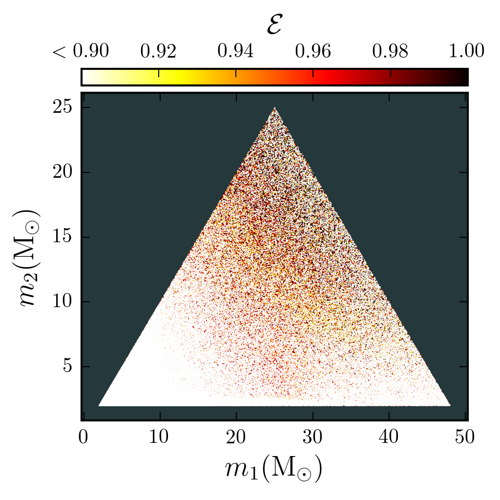
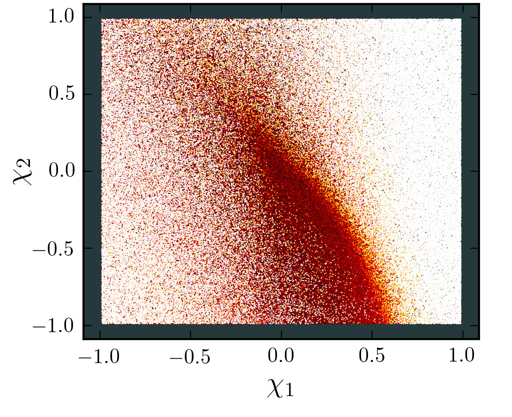
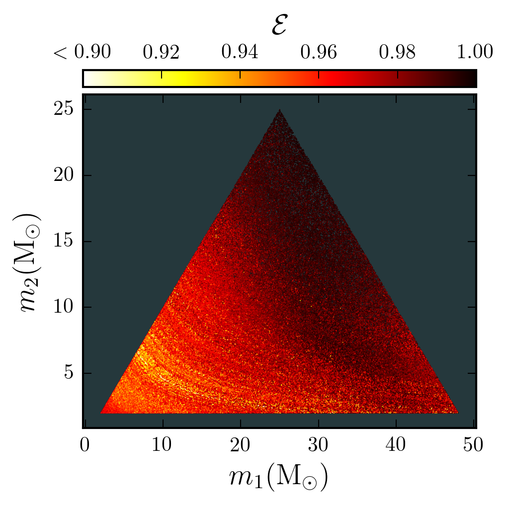
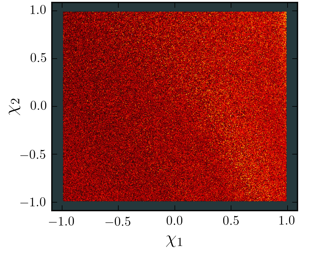
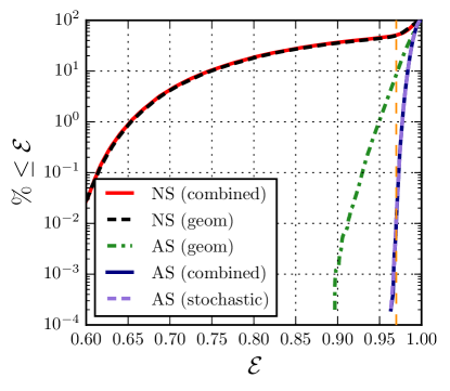
We plot the distribution of the effectualness over the set of simulated signals in Fig. 2. While the effectualness $\mathcal{E}$ of each simulated signal is useful for identifying areas of parameters space where a bank is not performing well, we wish to have a single value that describes the performance of the entire bank. For that, we do two additional comparisons. First, we find the percentage of signals that have $\mathcal{E}<0.97$, which is reported in Table 1. Second, we compute a weighted mean effectualness. Previous studies have used an “effective fitting factor” to assess the relative sensitivity of a bank, defined as Buonanno et al. (2003) $\left<\mathcal{E}^{3}\rho_{\textrm{opt}}^{3}\right>/\left<\rho_{\textrm{opt}}^{3}\right>$, where the mean is taken over the set of simulated signals. The effective fitting factor gives an approximate estimate of the fraction of signals that are detected by a bank assuming that signals are distributed uniform in volume. However, we have found that when considering a large range in masses, as we do in this study, a few high-mass signals can dominate the effective fitting factor, even when using a simulated signal that is log distributed in the component masses. This is because the amplitude of a signal scales approximately by $\mathcal{M}^{5/6}$, where $\mathcal{M}=M_{\mathrm{total}}(m_{1}m_{2}/M^{2}_{\mathrm{total}})^{3/5}$ is the chirp mass of the signal. Thus, the larger the chirp mass of a signal, the larger its optimal SNR. To give equal weight to lower-mass signals, we define the weighted mean effectualness $\left<\mathcal{E}_{w}\right>$ as:

$$\left<\mathcal{E}_{w}\right>=\frac{\left<(\mathcal{E}\mathcal{M}^{-5/6}\rho_{\textrm{opt}})^{3}\right>}{\left<(\mathcal{M}^{-5/6}\rho_{\textrm{opt}})^{3}\right>}.$$ (10)

These values are also reported in Table 1.

We use waveform models from double-spin BBH mergers built within the effective-one-body formalism, notably the non-precessing (or “aligned”) spin templates developed in Ref. Taracchini et al. (2014). The waveforms describe the full coalescence process, i.e., inspiral, merger and ringdown, but include only the main spin-weighted spherical-harmonic mode, i.e., the $(2,2)$ mode. Henceforth, we shall refer to those waveforms as SEOBNRv2 templates.

II.2 Non-spinning template banks

Template bank	Size	$\%$ of signals with $\mathcal{E}<0.97$	$\left<\mathcal{E}_{w}\right>$
Non-spinning geometric	7 734	50	0.738
Non-spinning combined	8 935	51	0.737
Aligned-spin geometric	57 177	8.5	0.954
Aligned-spin stochastic	64 318	0.01	0.970
Aligned-spin combined	60 766	0.01	0.970

Table 1: The sizes of the various template banks constructed in Sec. II. The non-spinning and aligned-spin combined banks refer to banks constructed using both the geometric and stochastic algorithms, as discussed in Sec. II.5.

The template placement algorithms that were used for creating banks of non-spinning signals for previous compact-object binary searches in LIGO and Virgo data are described in Refs. Sathyaprakash and Dhurandhar (1991); Poisson and Will (1995); Balasubramanian et al. (1996); Owen (1996); Owen and Sathyaprakash (1999); Babak et al. (2006); Cokelaer (2007). This method requires an analytical prediction of the mismatch between two nearby waveforms to create a parameter-space metric describing how far apart two points must be in the parameter space of the two masses before their overlap drops to a specified value. This approximation is only valid for overlaps close to 1, but has been found to be a very useful tool when creating banks with a minimal-match of 0.97. For bank construction the parameter space metric must be constant—or almost constant—over the whole parameter space. Currently such a metric only exists for the inspiral-only “TaylorF2” waveform approximant and requires the assumption that the termination frequency of the waveform will be constant over the parameter space Babak et al. (2006); Brown et al. (2012); Keppel et al. (2013). With this TaylorF2 parameter space metric it is possible to place a regular hexagonal lattice in the two-dimensional, non-spinning parameter space that covers the entire space at a desired minimal match Cokelaer (2007).

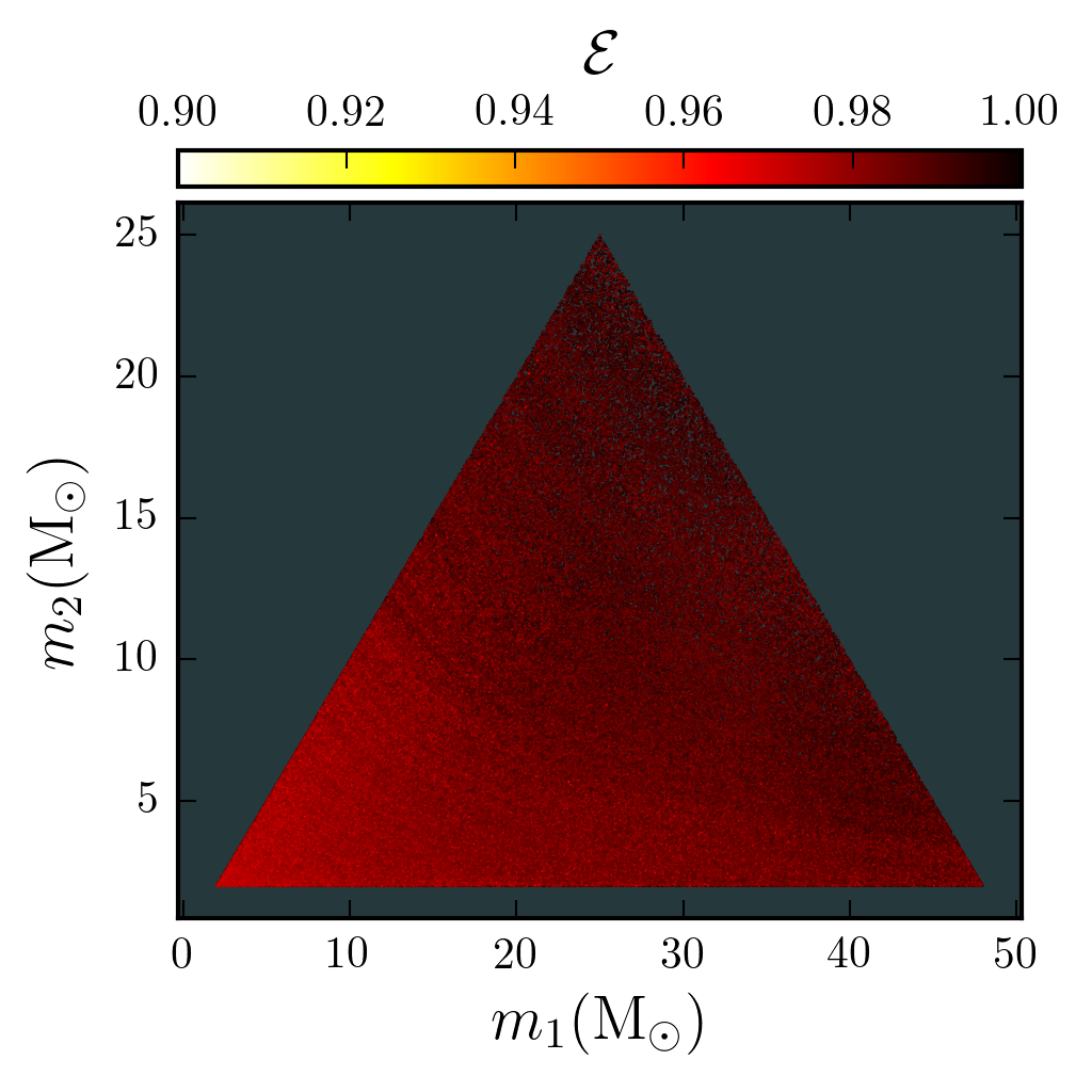
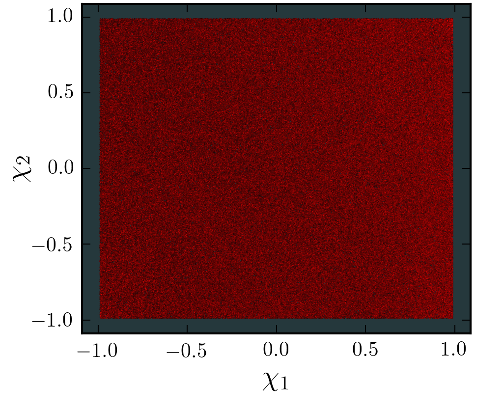
Using this traditional non-spinning template bank construction algorithm with the TaylorF2 parameter space metric, we generate a template bank of waveforms within the mass range described above and neglecting spin effects. Then, modelling all of the templates with the SEOBNRv2 waveform model, we compute the effectualness of this non-spinning template bank to SEOBNRv2 aligned-spin signals. The result of this is plotted in Figs. 1 and 2. The number of templates in this bank—7 734—and all other banks described in this section are listed in Tab. 1. It can clearly be seen from Fig. 2 that a large number of signals were recovered with the non-spinning bank with effectualness less than 0.97. Indeed, roughly 30% of signals have $\mathcal{E}<0.9$. We translate this into detection volume, compare this with our aligned-spin banks and assess performance in different regions of the mass-spin parameter space later in the work. However, this plot indicates that an aligned-spin bank could offer a significant improvement in detection rate.

II.3 Geometric algorithm

In Refs. Brown et al. (2012); Harry et al. (2014) the authors extended the non-spinning geometric approach to include aligned-spin signals for binary neutron star and neutron-star black-hole template bank placement, allowing for the higher dimensionality of the aligned-spin parameter space. However, geometric placement requires a parameter space that is globally flat. Efficient lattice algorithms are not known for general, intrinsically curved, parameter spaces Conway and Sloane (1993). To obtain a parameter space metric that is constant over the whole parameter space, we must use the inspiral-only TaylorF2 parameter space metric, and assume that all waveforms terminate at the same fixed frequency Brown et al. (2012). For binary neutron-star signals this is a valid approach as the merger occurs at a frequency outside of the range of sensitivity for ground-based interferometers Brown et al. (2012). However, for BBH signals, the parameter space is large and these assumptions are not valid for template bank placement, as we will demonstrate. For non-spinning bank placement this approach is equally invalid, but generally it produces template over-coverage in the high-mass parameter space. As the template density is low anyway in the high-mass parameter space, this results in effectual template banks with only a small amount more template waveforms than are needed. However, when considering aligned-spin systems there is a strong degeneracy between mass ratio and the spins, which can be broken when waveforms terminate at different frequencies. As the geometric approach cannot take this into account it can create template banks that are not effectual, as we will show below.

We construct a geometric aligned-spin bank to cover the parameter space using the TaylorF2 aligned-spin metric and choosing a fixed value for the waveform cut-off frequency of 1100Hz. We then test effectualness using the same set of points as for the non-spinning bank and again modelling the aligned spin templates and signal waveforms using the SEOBNRv2 waveform model. The results of this are also shown in Figs. 1 and 2. This bank contains 57 177 templates. We can see that the effectualness for this aligned-spin bank is much closer to the desired minimal-match criterion of $>0.97$, however there are regions of parameter space where the minimal match can be as low as 0.9. The geometric approach offers us an efficient way of covering the low-mass parameter space, but is not effectual everywhere when considering broad parameter spaces.

(a) Non-spinning: geometric-only

(b) Aligned-spin: geometric-only

(c) Aligned-spin: combined

Figure 1: Effectualness ($\mathcal{E}$) as a function of $m_{1},m_{2}$ (top) and $\chi_{1},\chi_{2}$ (bottom) of the non-spinning bank, the aligned-spin geometric-only bank, and the aligned-spin with geometric and stochastic placement bank. Each point represents a simulated signal.

Figure 2: Cumulative histogram of the effectualness ($\mathcal{E}$) of each bank. The y-axis shows the percentage of simulated signals that have $\mathcal{E}\leq$ the value given on the x-axis. The vertical orange line shows the desired minimal-match of the banks ($=0.97$).

II.4 Stochastic algorithm

An alternative method for placing banks of aligned-spin systems is the stochastic algorithm. In this method one randomly places a large set of points in the parameter space and then iterates over these points accepting each point into the template bank only if its overlap with all points already accepted to the template bank is less than the minimal match. This method was first proposed in the context of the LISA space-based detector Harry et al. (2009); Babak (2008), and has been adapted to the problem of aligned-spin template placement for LIGO and Virgo searches in Refs. Ajith et al. (2014); Privitera et al. (2014). This method can only guarantee that all points of the parameter space are covered to the minimal-match criterion if an infinite number of seed points are used. Therefore some approximation to the minimal-match criterion must be used, such as limiting the total number of seed points, or terminating the iterative process after a specific number of points have been rejected in succession. The stochastic algorithm uses more templates to cover a parameter space than the geometric approach, and can be computationally expensive when the overlaps are computed explicitly. However, this method offers a general approach that can be used to place a template bank for any parameter space.

Applying the stochastic method directly to our aligned-spin parameter space is computationally expensive. In order to optimize this process and speed up the generation of an aligned-spin template bank in this parameter space we make use of two new optimizations, in addition to the methods described in Refs. Ajith et al. (2014); Privitera et al. (2014).

The value of the frequency spacing used in the matched-filter integral ($df$) is normally chosen to be $1/L$, where $L$ is the closest power-of-2 that is greater than the length of the waveform (in seconds). This is sufficient to measure the overlap between two waveforms in a time window of $L$ seconds. However, for bank generation we are only interested in the maximum overlap between two waveforms. If the two waveforms are aligned so that their peak amplitudes occur at the same time, the maximum overlap is near to the time point corresponding to 0 displacement between the two waveforms. Therefore, we can increase the value of $df$, which reduces the cost of the inverse Fourier transform used to obtain the overlap as a function of time. To be sure that the value of $df$ is not set so large that an incorrect overlap is obtained we compute the overlap using some initial value of the frequency spacing ($df_{0}$) and also compute a second overlap using $df_{0}/2$. If both overlaps agree to within 1%, or if either overlap is less than four times the difference between the minimal match and unity—0.88 in this case—we use that value. Otherwise the overlap is computed again at $df_{0}/4$ and compared to the value obtained at $df_{0}/2$. This process continues iteratively until the value of the overlap converges. In our testing we found that $df_{0}=4$Hz was a suitable choice and that is used in the numbers and results quoted below. In this manner, we reduce the cost of computing overlaps, and can quickly assess cases where the overlap between two waveforms is small. This significantly reduces the computational cost of the stochastic bank. A similar approach has also been employed in the context of parameter estimation to achieve a similar speedup in computational time Pürrer et al. (2015).

In the approach described in Refs. Ajith et al. (2014); Privitera et al. (2014) the stochastic step must be parallelized due to computational cost. This is done by splitting the parameter space into a number of non-overlapping chirp-mass bins and running the stochastic bank generator individually on each chirp-mass region. Each individual job places points until a specified number of points, 100 000 in our case, were rejected while accepting the last 10 templates into the bank. This parallelization results in some over coverage along the chirp-mass boundaries and so the number of chirp-mass bins must be chosen to balance this over coverage against the computational cost of generating the bank. We investigated using varying numbers of non-overlapping chirp-mass regions and found that in this case 25 regions provided the best balance between these two factors. However, we note that the majority of the computational cost associated with the stochastic algorithm is spent accepting the final small number of templates Harry et al. (2009). We therefore organize the stochastic placement in two steps. First, we run a single instance of the stochastic generator, covering the full parameter space, but have it terminate when only 2500 points have been rejected in accepting the last 10 templates. Then this semi-complete stochastic bank can be used as a seed to the parallel generation to ensure completeness while minimizing double coverage along the boundaries of the chirp-mass bins.

We construct an aligned-spin stochastic template bank using these methods and again test the effectualness of this bank using the same set of test points as before. This bank contains 64 318 templates, which can be compared with the 57 177 templates that the geometric algorithm placed. However, in Fig. 2 we can see that the stochastic bank more completely covers the parameter space, with only 0.01% of points in the parameter space having an effectualness less than 0.97.

II.5 A combined geometric-stochastic approach

The geometric and stochastic placement methods both offer their own advantages and disadvantages when applied to bank placement for BBH signals for aLIGO and advanced Virgo. Previous works have always focused on using one method or the other Harry et al. (2014); Privitera et al. (2014). Here we propose that the best results are found if we combine the two methods together. Specifically we propose that template banks for BBH searches in aLIGO and advanced Virgo take the following approach. First, generate a bank using the aligned-spin geometrical lattice up to some total mass for which the placement is valid. For the early aLIGO noise curve that we consider here, we have empirically determined that a boundary on the total mass of 6 $M_{\odot}$ provides a suitable boundary at which to stop the geometric approach. Second, we use the stochastic algorithm, except, instead of starting with an empty template bank, we start with the aligned-spin geometric bank and test points in parameter space against this “seed” bank. No mass limits are given to the stochastic algorithm and it ensures that the full parameter space is covered, including any “holes” that might have been left in the original geometric template bank.

As with the other banks in this section we compute effectualness using the set of test points described at the top of this section. This bank contains 60 766 points and the distribution of effectualness can be seen in Figs. 1 and 2. We can see that in this case only 0.01% of the test points have a $\mathcal{E}<0.97$; the lowest value in our set of 500 000 points is at a minimal match of 0.964. As mentioned above this is consistent with the stochastic algorithm, which cannot guarantee that 100% of points has minimal match greater than some threshold. As a balance between template number and signal recovery we recommend that this combined method be used for producing banks of aligned-spin BBH template waveforms.

Finally, for completeness, we also generate a non-spinning bank combining both geometric and stochastic placement as described above. This allows us to make direct comparisons between the non-spinning and aligned-spin banks, generated using the same combination of the geometric and stochastic algorithms in the remainder of the paper. This bank contains 8 935 templates and is also plotted in Fig. 2. The performance of this bank when searching for aligned-spin signals is largely indistinguishable from the non-spinning bank generated using the traditional, geometric, method.

III Relative gain over non-spinning bank

Having arrived at an effectual aligned-spin template bank, we can now investigate the gain in sensitivity by using this bank in place of a non-spinning bank. To do this we estimate the sensitive volume, $\mathcal{V}$, for a search using each bank. The sensitive volume can be thought of as the mass-averaged volume in which a signal would be detected above a specific value of some ranking statistic $\hat{\rho}$. This can be written explicitly as

$$\mathcal{V}(\hat{\rho})=\int\epsilon(\hat{\rho};\mathbf{\Upsilon},\mathbf{\Xi},\mathbf{x})q(\mathbf{\Upsilon},\mathbf{\Xi},\mathbf{x})\mathrm{d}\mathbf{x}\mathrm{d}\mathbf{\Upsilon}\mathrm{d}\mathbf{\Xi}.$$ (11)

Here, $\mathbf{x}$ is the three-volume of space. For compactness, we let $\mathbf{\Lambda}=(\mathbf{\Upsilon},\mathbf{\Xi})$. The function $q(\mathbf{\Lambda},\mathbf{x})$ is the distribution of signals in the universe; i.e., it is the number of signals that exist in the universe per unit time. The efficiency $\epsilon(\hat{\rho};\mathbf{\Lambda},\mathbf{x})$ is the fraction of those signals that can be detected by the search at the given $\hat{\rho}$. For comparing pipelines, we will find it convenient to normalize $q$ such that if we integrate it over some fiducial spatial volume $V_{\max}$, we have:

$$\iint\int\limits_{V_{\max}}q(\mathbf{\Lambda},\mathbf{x})\mathrm{d}\mathbf{x}\mathrm{d}\mathbf{\Lambda}=V_{\max}.$$

We choose $V_{\max}$ such that the efficiency of the search is $0$ to any signal outside of $V_{\max}$.

The sensitive volume is dependent on the distribution of signals in the universe, $q$. For BBHs with total masses $\leq 50\,\mathrm{M}_{\odot}$, the detectors are sensitive out to a maximum distance of $\sim 1\,\mathrm{Gpc}$ assuming the early advanced LIGO PSD. Over these distances we can assume an isotropic distribution of signals Abadie et al. (2010b); i.e., we assume that signals are distributed uniformly in inclination, sky-location and orientation. The detection of GW150914 confirmed that BBHs with $M_{\mathrm{total}}\approx 65\,\mathrm{M}_{\odot}$ exist Abbott et al. (2016d), but beyond that, the mass and spin distribution of BBHs is largely unknown. For simplicity, in this study we assume an astrophysical prior that is uniform in component mass between $2$ and $25\,\mathrm{M}_{\odot}$ and uniform in aligned-spin magnitude. However, in the following sections we also produce sensitive volumes as a function component mass and spin, to mitigate the effects of choosing an inaccurate prior.

With these assumptions of the distribution of signals, we show in the appendix that the sensitive volume is approximately [see Eq. (24)]:

$$\mathcal{V}(\hat{\rho})\approx 4\pi\sum_{i}^{N}\tilde{w}_{i}\left[r_{\min,i}^{3}+3\Theta(\hat{\rho}_{i})\Delta r_{i}r_{i}^{2}\right],$$ (12)

where the sum is over the same simulated signals we used in Sec. II to assess the effectualness of each bank. The function $\Theta(\hat{\rho})$ equals one if a simulated signal has a ranking statistic $\geq\hat{\rho}$ and zero otherwise; the normalized weights $\tilde{w}_{i}$ are needed to convert from the simulated signals’ mass distribution ($\log$ in the component masses) to our assumed astrophysical distribution (uniform in the component masses) [see Eq. (25)]. Each signal’s distance $r_{i}$ is drawn uniformly between distance bounds $r_{\max,i}-r_{\min,i}\equiv\Delta r_{i}$.

The ranking statistic $\hat{\rho}$ is used to determine the likelihood that candidate events are GWs. We choose a threshold $\hat{\rho}^{\dagger}$ such that the probability of mis-identifying noise as a detection—the false alarm probability—is small. For larger template banks, searching larger regions of parameter space, the rate of background triggers above a given value of detection threshold increases. Therefore a template bank covering the aligned-spin parameter space has a larger false alarm probability $\mathcal{F}$ at fixed value of detection threshold than a non-spinning template bank. To keep the false alarm probability fixed, the threshold at which a detection could be claimed must therefore increase for the aligned-spin bank.

If the detector data were stationary Gaussian noise, the optimal (in the Neyman-Pearson sense) ranking statistic would be SNR. Real gravitational-wave detector data is not Gaussian. Due to the presence of non-Gaussian transients (glitches), signal-based vetoes are needed to separate glitches from real signal candidates Aasi et al. (2012, 2015). Several signal-based vetoes have been proposed Allen (2005); Hanna (2008); Harry and Fairhurst (2011). The signal-based veto used in the most recent searches for compact-object binary mergers Abadie et al. (2012); Aasi et al. (2013a), and the one we adopt here, is the $\chi^{2}$ test first proposed in Ref. Allen (2005). This statistic splits the template $h$ into $p$ non-overlapping frequency bins such that each sub-template $h_{i}$ contributes an equal amount to the SNR if the data exactly matches the template. Filtering each $h_{i}$ with the data, we can test how well the frequency evolution of the SNR matches the expected evolution with the statistic:

$$\chi^{2}=\frac{p}{\left<h,h\right>}\sum_{i=1}^{p}\left|\left<h_{i},s\right>-\frac{\left<h,s\right>}{p}\right|^{2}.$$ (13)

In Gaussian noise, this statistic is $\chi^{2}$ distributed with $2p-2$ degrees of freedom. The greater the mismatch between the data and the template the larger the $\chi^{2}$. This $\chi^{2}$ statistic as well as the SNR is then used to compute a detection statistic Abadie et al. (2012)

$$\tilde{\rho}=\left\{\begin{array}[]{cl}\rho&\text{for $\chi_{r}^{2}\leq 1$},\\ \rho\left[\frac{1}{2}\left(1+\left(\chi_{r}^{2}\right)^{\!3}\right)\right]^{-1/6}&\text{for $\chi_{r}^{2}>1$,}\end{array}\right.$$ (14)

where $\chi^{2}_{r}=\chi^{2}/(2p-2)$ is the reduced $\chi^{2}$. In this study we use $p=16$, as used in the search for compact-object binary mergers with total mass less than 25 $M_{\odot}$ in initial LIGO and initial Virgo’s last observing runs Abadie et al. (2012). We note that another choice for the number of $\chi^{2}$ bins can produce better sensitivity. In the search over the initial LIGO and Virgo data for binaries with total mass greater than $25\,\mathrm{M}_{\odot}$ $p=10$ was used Aasi et al. (2013a). However, further tuning of this parameter is outside the scope of this paper.

It has been shown Babak et al. (2013) that re-weighting the SNR via Eq. (14) down-weights glitches sufficiently such that the distribution of $\tilde{\rho}$ in noise is close to that of SNR in Gaussian noise. Conversely, $\tilde{\rho}\approx\rho$ for signals, as long as the mismatch between signals and templates is small. Therefore, the re-weighted SNR allows searches for compact-object mergers to reach comparable sensitivities to the ideal case where the detectors’ data is Gaussian. However, if templates do not match signals well, as in the case of the non-spinning bank searching for spinning signals, then the $\tilde{\rho}$ of those signals will be less than the raw SNR $\rho$. This reduces the sensitive volume of the non-spinning bank compared to what would be obtained if only $\rho$ was considered, as has been done in many other studies Brown et al. (2012); Privitera et al. (2014); Harry et al. (2014).

Searches for BBHs also require that candidate gravitational wave triggers occur in multiple detectors with the same mass and spins within the light-travel time between the detectors. In that case, the network re-weighted SNR for the search is computed from the quadrature sum of the single-detector $\tilde{\rho}$. The network re-weighted SNR is the ranking statistic $\hat{\rho}$ we use to compute the sensitive volume.

In the following section we compare the sensitive volumes of the aligned-spin bank to the non-spinning banks. In Sec. III.1 we use simulated Gaussian noise for each detector. In Sec. III.2 we run the full modern search pipeline described in Ref. Dal Canton et al. (2014) on a subset of the simulated signals using data from initial LIGO’s sixth science run (S6) recolored to resemble the predicted sensitivity of aLIGO’s first observing run.

III.1 Gaussian noise

As we will show below, the sensitive volume is strongly dependent on our choice of astrophysical prior. Higher-mass systems tend to dominate the sensitive volume estimate because they emit more power in gravitational waves. This is particularly true when assuming a prior that is uniform in component mass, as we have done here. We will obtain misleading results if our prior is wrong, which is likely given the large uncertainty in the mass and spin distribution of BBHs.

To mitigate the effect of our choice of prior, we wish to explore how the sensitive volume changes across masses and spins. Doing so requires a large number of simulated signals, as the variance in the volume estimate increases the more we sub-divide the parameter space. However, adding more than a few thousand simulated signals to real detector data and analyzing with the full search pipeline is computationally expensive, as it requires finding the overlap between every template and every simulated signal to find the best matching template in a particular realization of noise.

Instead, in this section we use Gaussian noise to approximate the average sensitive volume. By definition, the most effectual template to a signal will be the template that has the largest SNR when averaged over several realizations of Gaussian noise. We therefore do the following: we only filter each simulated signal with its most effectual template in $16$ realizations of simulated Gaussian noise in each LIGO detector. We find the network re-weighted SNR $\hat{\rho}$ in each realization, then average over the realizations to get a measurement of the expectation value of $\hat{\rho}$, $\left<\hat{\rho}\right>$. We use this to compute the sensitive volume. This allows us to use all $500\,000$ simulated signals from the previous section for computing sensitive volume.

Another advantage of using Gaussian noise is we can analytically estimate the increase in false alarm probability at fixed $\hat{\rho}$ of the aligned-spin bank as compared to the non-spinning bank. In real data the distribution of re-weighted SNR is not the same for all templates. The shorter the bandwidth of a template in the frequency domain, the larger its overlap with non-Gaussian transients. This causes shorter-bandwidth templates to produce triggers with large values of $\hat{\rho}$ at a higher rate than larger-bandwidth templates Babak et al. (2013). To account for this, searches have binned results by various parameters when estimating false alarm rate, then combined results over the bins Abadie et al. (2012); Aasi et al. (2013a). The choice of parameter to use and the size of bins adds an additional complication when comparing sensitivity, and is dependent on the noise.

However, in Gaussian noise, the SNR of every template is $\chi$ distributed with two degrees of freedom. We therefore do not need to worry about binning results by parameters. Furthermore, in Gaussian noise we can analytically estimate the increase in false alarm probability due to the larger parameter space covered by the aligned-spin bank. Let us assume that every template is independent of each other. With this assumption, if we have $N_{t}$ templates in a bank, the probability of getting one or more single-detector triggers with an SNR $\geq\rho$ is:

$$P(\rho|N_{t})=1-C_{\chi}(\rho)^{N_{t}},$$ (15)

where $C_{\chi}(\rho)=1-e^{-\rho^{2}/2}$ is the cumulative distribution function of the $\chi$ distribution with two degrees of freedom. In Gaussian noise with no signals, $\tilde{\rho}\approx\rho$; with two detectors, $\hat{\rho}\approx\sqrt{2}\tilde{\rho}$. We therefore model the false alarm probability as $\mathcal{F}(\hat{\rho})\approx P(\rho/\sqrt{2}|N_{t})$. If we have a bank with $N_{0}$ templates in which the threshold for detection is $\hat{\rho}_{0}$, then to keep the false alarm probability fixed in a bank with $N_{t}$ templates, $\hat{\rho}$ must increase to:

$$\hat{\rho}^{2}=-4\log\left[1-\left(1-e^{-\hat{\rho}_{0}^{2}/4}\right)^{N_{0}/N_{t}}\right]$$ (16)

Since templates are not actually independent this model does not give an accurate absolute value of $\mathcal{F}(\tilde{\rho})$. However, the model is adequate for comparing the relative false alarm probabilities of two banks that cover different size parameter spaces.

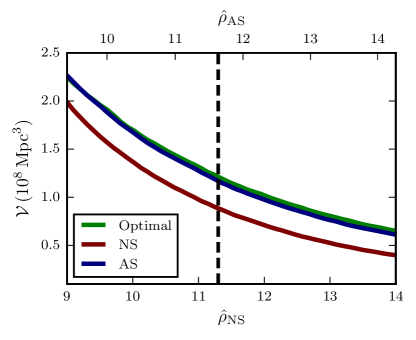
Figure 3 shows the sensitive volume versus network re-weighted SNR for each bank assuming an astrophysical prior that is uniform in component masses and spin-magnitude. The re-weighted SNR of the aligned-spin bank is offset with respect to the non-spinning bank via Eq. (16) to account for the increase in false alarm probability. Even so, we see that the aligned-spin bank is more sensitive than the non-spinning bank for all thresholds considered in the plot. Also plotted is the “optimal” sensitive volume, which is the sensitivity if every template matched every signal exactly, and the detection statistic was SNR. We see that the sensitivity of the aligned-spin bank with re-weighted SNR as the ranking statistic is close to optimal, as expected from the effectualness study in the prior section.

A single-detector SNR threshold of $\rho=8$ is typically assumed to be large enough to confidently claim a detection. For two detectors, this corresponds to $\hat{\rho}=\sqrt{N_{d}}\rho\approx 11.3$. We use this as the detection threshold for the non-spinning bank. By Eq. (16), this corresponds to a threshold of $\approx 11.7$ for the aligned-spin bank. We find that the aligned-spin bank is $1.30\pm 0.01$ more sensitive than the non-spinning bank at this threshold (dashed line in Fig. 3).

Figure 3: Sensitive volume versus re-weighted SNR $\hat{\rho}$ of the non-spinning (NS) and aligned-spin (AS) bank. The bottom axis shows $\hat{\rho}$ for the non-spinning bank; the top axis shows $\hat{\rho}$ scaled to account for the increase in false alarm rate of the aligned-spin bank. The “Optimal” volume shows the sensitive volume using the optimal SNR of each simulated signal as the detection statistic. The dashed line shows a threshold re-weighted SNR equivalent to a single-detector SNR threshold of $8$ in the non-spinning search ($\sim 11.3$ for NS; $\sim 11.7$ for AS).

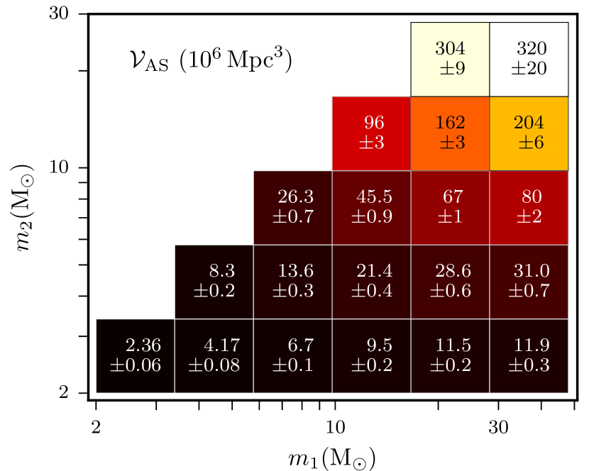
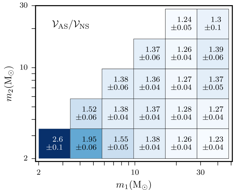
As stated above, the relative sensitivity of the two banks is strongly dependent on the astrophysical prior chosen. Indeed, because we have chosen a prior that is uniform in component masses, the average volume is dominated by high-mass signals. This can be seen in the left plot of Fig. 4, which shows the sensitive volume of the aligned-spin search sub-divided into bins in component mass. The sensitive volume of the highest mass tile is over two-orders of magnitude larger than the lowest-mass tile ($\sim 300\times 10^{6}\,\mathrm{Mpc}^{3}$ versus $\sim 2\times 10^{6}\,\mathrm{Mpc}^{3}$). Taking the ratio of the sensitive volumes of the aligned-spin bank to the non-spinning bank in each mass bin (right plot of Fig. 4), we find that the aligned-spin bank has a larger gain as we go to lower masses.

Figure 4: Left: Sensitive volume of the aligned-spin bank ($\mathcal{V}_{\mathrm{AS}}$) as a function of component mass. Right: Ratio of sensitive volumes of the aligned-spin bank to the non-spinning bank ($\mathcal{V}_{\mathrm{NS}}$) as a function of component mass. The threshold $\hat{\rho}$ used to compute sensitive volumes in these plots is 11.3 for the non-spinning bank and 11.69 for the aligned-spin bank (dashed line, Fig. 3).

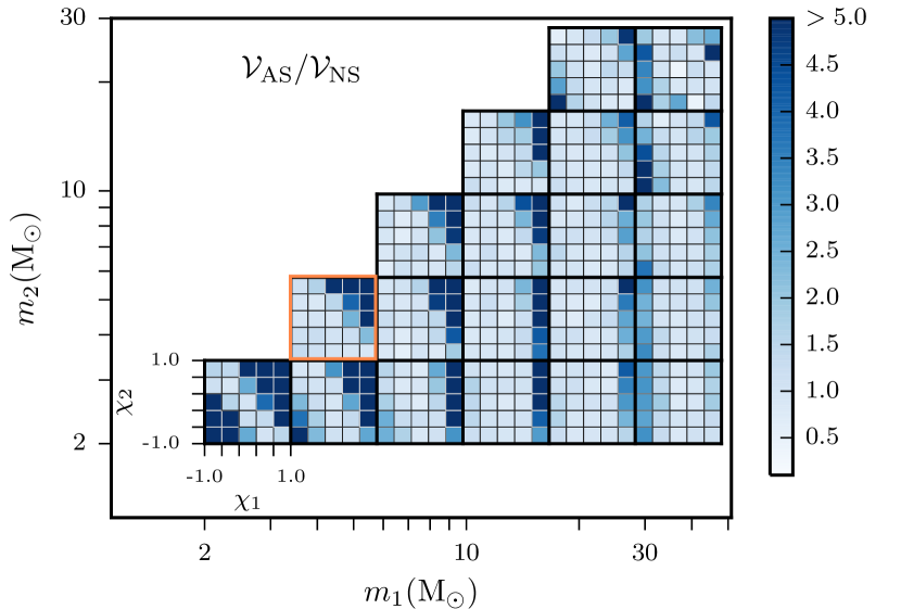
In Fig. 5 (left) we further sub-divide each mass tile into $25$ bins in $\chi_{1}$ and $\chi_{2}$, with the color bar indicating the relative sensitivity of the two banks. In the lowest-mass tile (bottom left corner), we see that the gain in sensitivity can be $>5$ when both spins are either $<-0.2$ (anti-aligned) or $>0.2$. As we move to higher mass tiles, however, the gain in the anti-aligned region approaches one, particularly for tiles that are close to the equal-mass line. This is likely due to the degeneracy between spin and the symmetric mass ratio $\eta=(m_{1}m_{2})/M_{\mathrm{total}}^{2}$. Namely, at lower masses for which the inspiral dominates the waveform, negative (positive) spins are degenerate with smaller (larger) $\eta$ Ohme et al. (2013). Signals with negative spins can therefore be recovered by the non-spinning bank by templates with smaller $\eta$, which corresponds to larger mass ratio. In the lowest-mass corner of the bank, the range in mass ratio is limited by our minimum component mass boundary of $2\,\mathrm{M}_{\odot}$. We expect that if we extended the component mass to lower masses, the resulting larger range in mass ratio would mitigate the non-spinning bank’s loss in sensitivity to anti-aligned spins. Indeed, in the full search a minimum component mass of $1\,\mathrm{M}_{\odot}$ is used to incorporate BNS and NSBH systems Abbott et al. (2016c).

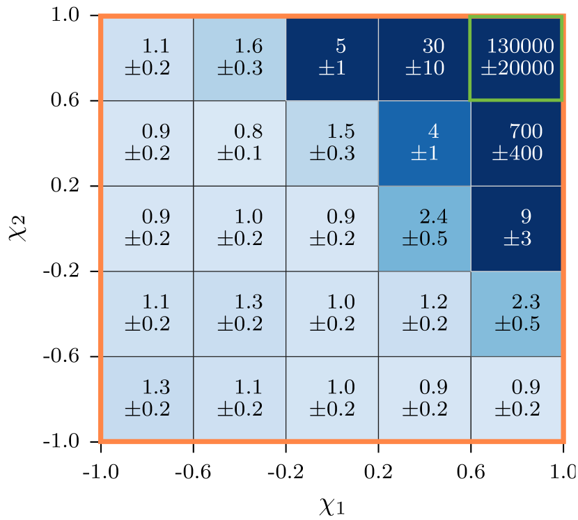
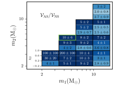
While the non-spinning bank’s loss in sensitivity to low-mass, anti-aligned signals can be mitigated by extending the bank’s boundaries to lower $\eta$, the same is not true for positive aligned-spins. This is because the symmetric mass ratio reaches a maximum at $0.25$, which corresponds to equal-mass systems. To extend the non-spinning bank to larger $\eta$ would require non-physical component masses. This is evident in Fig. 5: the gain in sensitivity remains $\gtrsim 5$ for component spins $\gtrsim 0.2$ and component masses $\lesssim 20\,\mathrm{M}_{\odot}$ even as the range in mass ratios spanned by the bank increases. This gain can be more than an order-of-magnitude when the component spins are $>0.6$. Indeed, if we zoom in on one of these low-mass tiles, $m_{1,2}\in[3.4,5.8)\,\mathrm{M}_{\odot}$ (highlighted box in the left plot), we find that aligned-spin bank is up to $O(10^{5})$ times more sensitive than the non-spinning bank for $\chi_{1,2}>0.6$ (highlighted tile in the right plot of Fig. 5). This is much larger than what is expected from SNR loss alone. The effectualness of the non-spinning bank is between $\sim 0.7$ and $\sim 0.6$ for this region of parameter space, indicating an SNR loss of $30$ – $40\,\%$. That would translate to a loss in sensitive volume of $66$ – $78\,\%$.

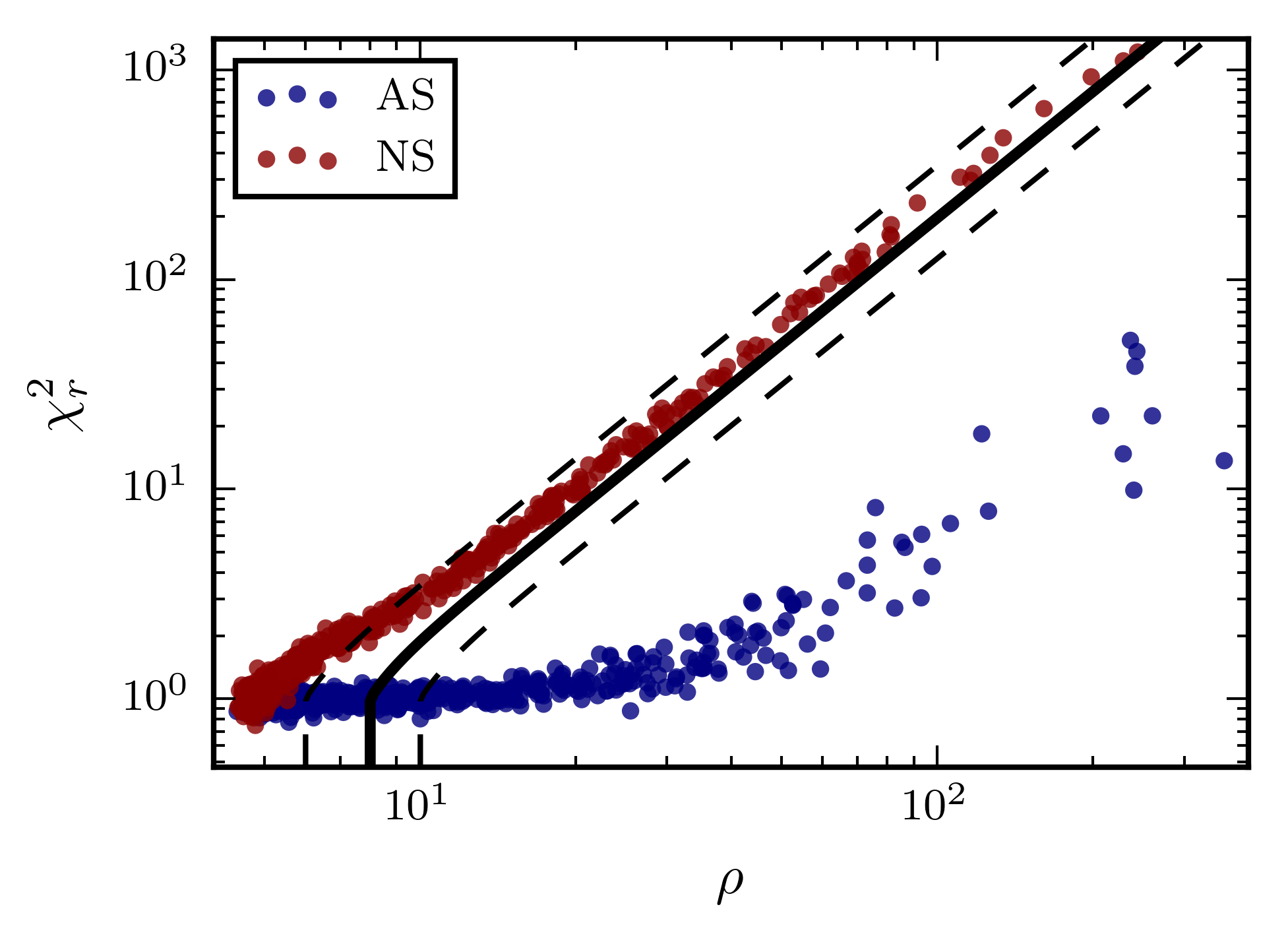
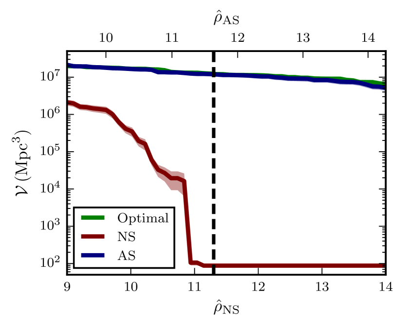
The reason for the large increase in sensitivity can be seen in the top plot of Fig. 6, which shows the reduced $\chi^{2}$ versus SNR in a single detector for this region of parameter space. We see that the $\chi_{r}^{2}$ of the signals when recovered by the non-spinning bank are quite large. In fact, the $\chi_{r}^{2}$ statistic asymptotes such that the re-weighted SNR of the signals is always $<8$ (solid black line in the figure). Thus, even when the optimal SNR of a signal is $400$ (and the recovered SNR by the non-spinning bank is $200$), the re-weighted SNR is still less than 8, which is the threshold for detection. This is strongly dependent on the threshold for detection: if the single-detector threshold was 6 (top dashed-line), these high-SNR events would be detected. This can be seen in the bottom plot of Fig. 6, which shows the volume versus threshold network re-weighted SNR for just this region of parameter space. We see that as the threshold decreases below 11.3 (corresponding to a single-detector SNR $=8$), the sensitivity of the non-spinning bank rapidly improves. For instance, at a threshold of $\tilde{\rho}=8$ (which corresponds to a single-detector SNR $\sim 5.6$), the gain is $\sim 3$, closer to that predicted by the loss in SNR.

The non-spinning sensitivity levels off at $\tilde{\rho}_{\mathrm{NS}}\sim 11$ in the bottom plot of Fig. 6 due to the minimum distance bound we used for the simulated signals. If we had chosen smaller bounds, the $\mathcal{V}_{\mathrm{NS}}$ would continue to drop, indicating that the non-spinning bank has zero sensitivity to these signals. We find similar characteristics for tiles in which the component masses are $<17\,\mathrm{M}_{\odot}$, $\chi_{1}\geq 0.6$, and $\chi_{2}\geq-0.2$.

By only filtering the most effectual template, we have made the assumption that $\left<\mathcal{V}(\hat{\rho})\right>\approx\mathcal{V}(\left<\hat{\rho}\right>)$. Figure 6 indicates that we are in a regime where small changes in $\chi_{r}^{2}$ have large effects on the sensitive volume. We expect that the approximation breaks down in this regime. The $\chi_{r}^{2}$ values of signals will fluctuate about the mean in different realizations of noise, which will cause small fluctuations in $\hat{\rho}$. For these low-mass, high-spin areas of parameter space, we expect these small fluctuations to be enough to occasionally bring $\hat{\rho}$ above threshold. Thus we do not expect the sensitive volume of the non-spinning bank to be exactly zero. In the next section we filter these low-mass, high-spin signals with the full template bank and pipeline to get a better estimate of the gain between the non-spinning bank and the aligned-spin bank in these regions of parameter space.

Figure 5: Left: Ratio of sensitive volumes of the aligned-spin bank ($\mathcal{V}_{\mathrm{AS}}$) to the non-spinning bank ($\mathcal{V}_{\mathrm{NS}}$) as a function of component mass and spin. Each mass tile is subdivided into $25$ tiles of the dimensionless spin of each component ($\chi_{1,2}$, inset axes). Dark blue tiles indicate regions in which the gain is $>5$. Right: The relative gain as a function of $\chi_{1}$ and $\chi_{2}$ for the mass bin $m_{1,2}\in[3.4,5.8)\,\mathrm{M}_{\odot}$ (highlighted mass tile in the left plot). The threshold re-weighted SNR used to compute sensitive volume in these plots is 11.3 for the non-spinning bank and 11.7 for the aligned-spin bank (dashed line, Fig. 3).

Figure 6: Single-detector SNR ($\rho$) versus reduced $\chi^{2}$ (top), and sensitive volume versus threshold $\hat{\rho}$ (bottom) for signals with $m_{1,2}\in[3.4,5.8)\,\mathrm{M}_{\odot}$ and $\chi_{1,2}\geq 0.6$ (the highlighted tile in the bottom plot of Fig. 5). The dashed lines in the top plot show lines of constant single-detector re-weighted SNR; the thick solid line shows a re-weighted SNR $=8$, which is the threshold we used for the non-spinning bank.

III.2 Recolored noise

To get a better estimate of the gain in sensitivity we can expect between the aligned-spin and non-spinning banks, we add simulated signals to S6 data recolored to resemble early advanced LIGO data. We analyze that data using the search algorithm described in Refs. Dal Canton et al. (2014); Usman et al. (2015). That is, we filter each signal with all templates, find coincidence, maximize over the bank using network re-weighted SNR, and estimate the background to find $\mathcal{F}(\hat{\rho})$. Since this is computationally expensive to perform on all $500\,000$ simulated signals, we limit this study to areas of parameter space where the gain in sensitive volume was $\gg 5$ in the previous section. Namely, we restrict to signals with $m_{1,2}<17$, $\chi_{1}>0.6$, and $\chi_{2}>-0.2$, of which there are $\sim 10\,000$.

As discussed in the last section, due to the presence of glitches, the distribution of $\hat{\rho}$ is not the same for all templates in real noise, as it is in Gaussian noise. Results are typically binned by some parameter Abadie et al. (2012); Aasi et al. (2013a) when estimating false alarm probability for this reason. For example, in Ref. Abadie et al. (2012), three bins in chirp mass were used. We do not try to do any binning here. This means that our results may not be as optimal, but we expect such binning to have a small effect on the relative gain in sensitivity between the non-spinning and aligned-spin bank.

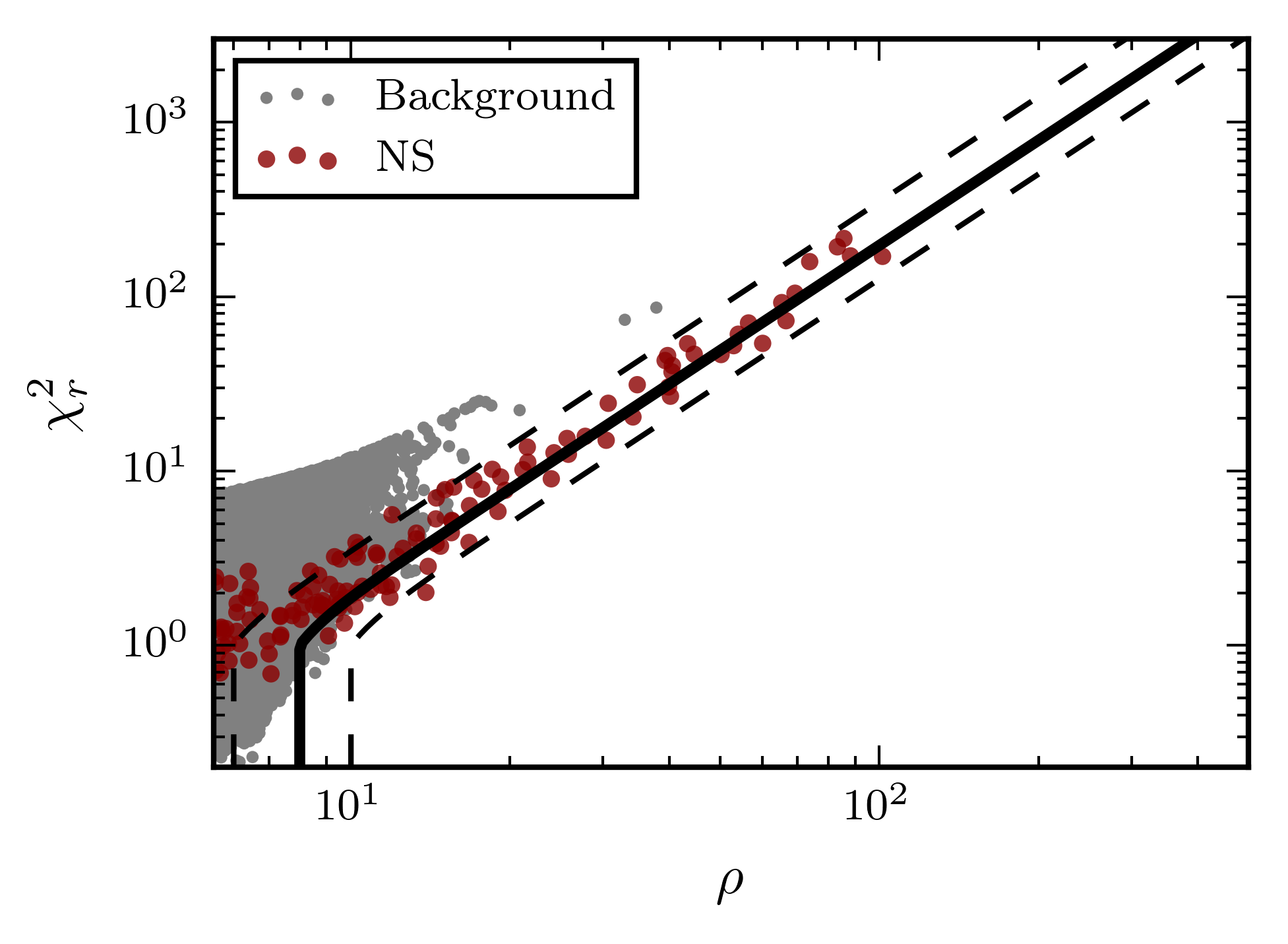
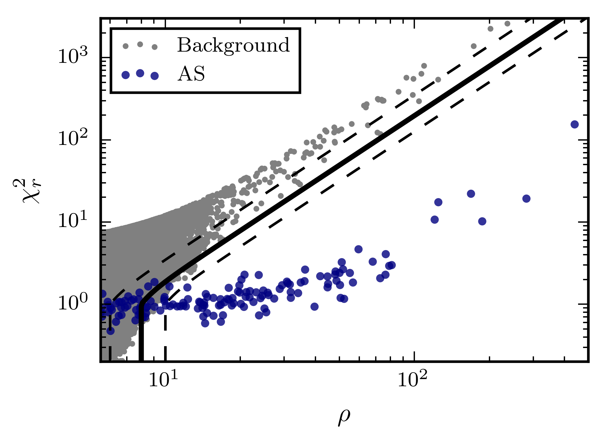
Figure 7 shows the relative gain between the non-spinning bank and the aligned-spin bank in the recolored noise. As expected, the gain is not as large as we found in the previous section. For example, focusing on the same region of parameter space that we highlighted in the prior section ($m_{1,2}\in[3.4,5.8)\,\mathrm{M}_{\odot}$ and $\chi_{1,2}\geq 0.6$) the gain is $10\pm 6$ (highlighted tile in Fig. 7). The reason for this can be seen in Fig. 8, which shows reduced $\chi^{2}$ versus SNR in a single detector for these signals when recovered by the non-spinning bank (top) and the aligned-spin bank (bottom) in the recolored noise. We find similar behavior as in the Gaussian noise results (Fig. 6): the $\chi^{2}$ of the signals when recovered by the non-spinning bank is large, causing the signals to asymptote to lines of constant re-weighted SNR. Even so, the variance of the reduced $\chi^{2}$ causes some signals to have re-weighted SNRs greater than the threshold of 8. The result is the non-spinning bank does recover at least some of the signals, yielding a non-zero sensitive volume. However, the sensitive volume of the aligned-spin bank in these areas of parameter space can still be an order-of-magnitude or larger than the non-spinning bank, which is larger than one might expect from SNR loss alone.

Triggers caused by noise are also shown in Fig. 8 (gray dots in both plots). These triggers form the background with which false alarm probability is measured. To improve the sensitivity of the non-spinning bank, one might consider changing the exact form of the $\chi^{2}$ re-weighting of the SNR used in Eq. (14). However, this would be difficult to do without also promoting noise triggers to higher significance. The large mismatch between the non-spinning templates and the spinning signals makes it difficult to separate glitches from signals. Contrast this to the aligned-spin bank. Although the number of noise triggers has increased, there continues to be good separation between the aligned-spin signals and noise. We conclude that the aligned-spin bank can be implemented using the same form of the re-weighted SNR given in Eq. (14).

Figure 7: Ratio of sensitive volumes of the aligned-spin bank ($\mathcal{V}_{\mathrm{AS}}$) to the non-spinning bank ($\mathcal{V}_{\mathrm{NS}}$) as a function of component mass and spin in the recolored noise. Tiles are only shown for the simulated signals that were selected for this test ( $\chi_{1}>0.6,~{}\chi_{2}\in[-0.2,0.99),m_{1,2}<16.6\,\mathrm{M}_{\odot}$). The highlighted tile corresponds to the same region of parameter space as the highlighted tile in the right plot of Fig. 5.

Figure 8: Single-detector SNR ($\rho$) versus reduced $\chi^{2}$ for the non-spinning (top) and aligned-spin (bottom) banks in recolored noise for signals with $m_{1,2}\in[3.4,5.8)\,\mathrm{M}_{\odot}$ and $\chi_{1,2}\geq 0.6$ (the highlighted tile in the right plot of Fig. 5) Also shown are the false alarms from each search (gray dots).

IV Conclusions

We have demonstrated here a complete method for conducting a search for GWs from BBH using an aligned-spin template bank in advanced LIGO. We have covered the parameter space combining two previously proposed methods for template placement: geometric and stochastic. We have shown that combining these methods yields a more effectual template bank than the geometric method alone, while also using $\sim 5\%$ fewer templates than the stochastic method alone. We expect that the savings will only increase as the lower-frequency performance of the LIGO detectors improves in future observing runs.

Applying the template bank to an analysis of simulated advanced LIGO data, we have characterized the improvement in sensitivity of the pipeline towards aligned-spin signals. We have found that the aligned-spin bank is significantly more sensitive than the non-spinning bank to signals with $\chi_{1}\gtrsim 0.6$ and component masses $m_{1,2}\lesssim 20\,\mathrm{M}_{\odot}$. From mismatch alone, we would expect the aligned-spin bank to have a sensitive volume that is $20$ to $30\%$ larger than the non-spinning bank in this region of parameter space. However, when the effects of $\chi^{2}$ re-weighting of SNR are included, we find that the aligned-spin bank can be one to two orders-of-magnitude more sensitive to these signals. Although less pronounced, the aligned-spin bank is also more sensitive to higher-mass systems with non-zero spins, with gains of $30-500\%$.

Due to the increase in false alarm rate, adding the aligned spin templates does reduce the sensitivity to non-spinning systems by $\sim 10\%$. However, this would only lead to a loss in detection rate if nearly all systems in the universe were non-spinning. Based on observations of X-ray binaries  McClintock et al. (2006); Gou et al. (2011, 2010, 2009); Miller et al. (2009); Valtonen et al. (2010); Martocchia et al. (2002) and population synthesis models Belczynski et al. (2008) we expect many systems to have spin. The significant gain in sensitivity to spinning systems therefore compensates for the relatively small loss in sensitivity to non-spinning systems.

Although we only considered BBHs with total mass $\leq 50\,\mathrm{M}_{\odot}$ in this study, the template-placement methods discussed here can be applied to a larger range of masses. We expect the gain in sensitivity to become less dramatic for signals with total masses $>50\,\mathrm{M}_{\odot}$, even if $\chi_{1}\gtrsim 0.6$. This is because $\chi^{2}$ becomes less effective at higher masses, in which the bandwidth of templates is short.

In order to arrive at these results we used the same tuning as was used in the search for CBCs in the sixth science run of initial LIGO Abadie et al. (2012). Namely, we used $16$ bins when computing $\chi^{2}$, and we used Eq. (14) to re-weight SNR. Due to the large $\chi^{2}$ values, we found that the sensitivity of the non-spinning bank can vary dramatically with small changes in the threshold $\hat{\rho}$ used to detect signals. Although another choice of $\chi^{2}$ bins and re-weighting is possible, it would be difficult to improve the sensitivity of the non-spinning bank without decreasing the ability of the search to separate signals from glitches. This is due to the large mismatches involved between non-spinning templates and spinning signals. The simplest, safest approach is to simply use aligned-spin templates in the search.

An aligned-spin template bank was used in the modeled search that found GW150915 Abbott et al. (2016a, c) that used the combined geometric and stochastic placement method discussed here. While GW150914 did not have very large spin — its effective spin was estimated to be $-0.06\pm 0.18$ Abbott et al. (2016d) — future detections may yield black holes with significant spin.

V Acknowledgements

We are grateful to Sukanta Bose, Thomas Dent, Chad Hanna, Andrew Lundgren, Alex Nielsen, and Alex Nitz for providing insightful discussions. The authors would also like to thank the Max Planck Gesellschaft for support. All calculations were carried out on the ATLAS and VULCAN clusters at the Albert Einstein Institute in Hannover and Potsdam, Germany, respectively.

Appendix A Derivation of sensitive volume

The integrand of Eq. (11) is a complicated function of the integration variables; the efficiency, for example, depends on the characteristics of the data and how well the ranking statistic $\hat{\rho}$ separates noise from signal, which is not known a priori. We therefore find the sensitive volume by Monte Carlo integration, as follows.

First, note that the efficiency function serves to determine what fraction of the total number of signals are detected. For example, if the universe contained $N$ signals within volume $V_{\max}$ (i.e., $q$ was a series of $N$ delta functions), $n$ of which are detected by a pipeline at some threshold $\hat{\rho}$, then the sensitive volume would be $nV_{\max}/N$. Assume then that we have $N$ random simulated signals drawn from the same distribution as $q$, which we filter through the pipeline to acquire a ranking stat value $\hat{\rho}_{i}$ for each. We can replace $\epsilon$ with a step function $\Theta$ such that $\Theta(\hat{\rho})=1$ if $\hat{\rho}\geq\hat{\rho}_{i}$, and 0 otherwise. The sensitive volume is then:

$$\mathcal{V}(\hat{\rho})\approx V_{\max}\frac{1}{N}\sum_{i}^{N}\Theta(\hat{\rho})=V_{\max}\left<\Theta(\hat{\rho})\right>,$$ (17)

The error in this estimate is given by the square root of the variance:

$$\delta\mathcal{V}=V_{\max}\sqrt{\frac{\left<\Theta^{2}\right>-\left<\Theta\right>^{2}}{N}}.$$ (18)

As discussed in the main text, for BBHs with total masses $\leq 50\,\mathrm{M}_{\odot}$, the LIGO detectors are sensitive out to a maximum distance of $\sim 1\,\mathrm{Gpc}$ assuming the early advanced LIGO PSD. Over these distances we assume an isotropic distribution of signals. Thus for Eq. (17) to be correct, we have to draw our simulated signals from a spatial distribution that is uniform in volume. However, due to the antenna pattern of the detectors, we have found that using a distribution uniform in volume causes most of the signals to be too weak to be detected by the pipeline. This leads to a large variance in the volume estimate. A more efficient approach is to do importance sampling, i.e., to draw the simulated signals from a distribution $q^{\prime}$ such that the majority of the signals closely straddle the boundary between being detected (found) and not being detected (missed).

In general, any Monte Carlo integral of a function $f$ over some volume $V$ can be written Press et al. (2007):

$$I=\int\limits_{V}f(\mathbf{x})q(\mathbf{x})\mathrm{d}\mathbf{x}=\int\limits_{V}g(\mathbf{x})q^{\prime}(\mathbf{x})\mathrm{d}\mathbf{x},$$ (19)

where $g(\mathbf{x})=f(\mathbf{x})q(\mathbf{x})/q^{\prime}(\mathbf{x})$. Here, $q$ is the distribution that is uniform in $V$ and $q^{\prime}$ is any other distribution from which we would prefer to draw samples. In order to approximate this as an average over $N$ random points sampled from $q^{\prime}$ we need to transform to the coordinate system $\mathbf{x}^{\prime}$ in which $q^{\prime}$ is uniform. Let $s^{-1}$ be the transformation from $\mathbf{x}^{\prime}$ to $\mathbf{x}$, such that $s(\mathbf{x}^{\prime})=\mathbf{x}$, and $|\mathbf{J}|$ be the Jacobian determinant of the transformation (i.e., $J_{ij}=\partial x^{\prime}_{i}/\partial x_{j}$). The integral is then the weighted average:

$$I =\int g\left(s[\mathbf{x}^{\prime}]\right)q\left(s[\mathbf{x}^{\prime}]\right)|\mathbf{J}|\mathrm{d}\mathbf{x}^{\prime}$$

$$\approx\sum_{i=1}^{N}\tilde{w}_{i}f\left(s[\mathbf{x}^{\prime}_{i}]\right)\equiv\left<f\right>_{w}$$ (20)

where:

$$\tilde{w}_{i}=\frac{w_{i}}{\sum_{j=1}^{N}w_{j}};\quad w_{i}=\frac{q\left(s[\mathbf{x}^{\prime}]\right)|\mathbf{J}|}{q^{\prime}\left(s[\mathbf{x}^{\prime}]\right)}.$$ (21)

This has error $\sqrt{(\left<f^{2}\right>_{w}-\left<f\right>_{w}^{2})/N}$ Gatz and Smith (1995).

We apply this to the spatial part of the sensitive volume integral as follows. First, we assume that within some minimum distance $r_{\min}$ nearly all signals will be detected by the pipeline at our detection threshold $\hat{\rho}^{\dagger}$. Likewise, due to noise, we know that all signals beyond some maximum distance $r_{\max}$ will not be detected by the pipeline. We determine these bounds based on the optimal network SNR. The optimal network SNR $\rho_{\mathrm{opt}}$ of a signal with some intrinsic and extrinsic parameters $\mathbf{\Lambda}^{*}$ is related to its physical distance $r$ via:

$$r=\frac{\sqrt{\sum_{i}\left<h_{i}(\mathbf{\Lambda}^{*}),h_{i}(\mathbf{\Lambda}^{*})\right>}}{\rho_{\mathrm{opt}}},$$ (22)

where $h_{i}$ is the strain caused by the signal at a fiducial distance of $1\,$Mpc in the $i$th detector, and the sum is over the number of detectors. If $\hat{\rho}=\rho_{\mathrm{opt}}$, then we know that the signal would be missed (found) at distances greater (less) than the distance corresponding to $\rho_{\mathrm{opt}}=\hat{\rho}^{\dagger}$. However, due to the mismatch between signal and template, $\chi^{2}$ re-weighting, and the presence of noise, $\hat{\rho}$ is not exactly equal to $\rho_{\mathrm{opt}}$. We therefore choose a maximum and minimum $\rho_{\mathrm{opt}}$ that we are confident bounds $\hat{\rho}^{\dagger}$. We then obtain a minimum and maximum distance bound for each simulated signal via Eq. (22). In this study, our detection threshold is $\hat{\rho}^{*}=8\sqrt{2}$; we conservatively choose a maximum (minimum) $\rho_{\mathrm{opt}}/\sqrt{2}$ of 400 (4) to obtain the distance bounds. Note that this means that $r_{\min}$ and $r_{\max}$ depend on the intrinsic and extrinsic parameters of the signal.

Given the distance bounds, we next choose a distribution to draw the distances from, $q^{\prime}$. This choice is informed by our assumed distribution of signals $q$. As discussed in the main text, for this study we assume an isotropic distribution of signals in the universe; i.e., we assume that $q$ is independent of $\mathbf{x}$. Given this distribution of signals and our choice of distance bounds, we have found that using a distribution $q^{\prime}$ uniform in the solid angle $\Omega$ and uniform in distance yields volume estimates with reasonably small variance. Thus for $r\in[r_{min}(\mathbf{\Lambda}),r_{\max}(\mathbf{\Lambda}))$,

$$q^{\prime}(\mathbf{\Lambda},r)=[r_{\max}(\mathbf{\Lambda})-r_{\min}(\mathbf{\Lambda})]^{-1}\equiv\Delta r(\mathbf{\Lambda}).$$

Since $q^{\prime}$ is uniform in $r$ and $\Omega$, the Jacobian determinant $|\mathbf{J}|=r^{2}$. With these choices, the sensitive volume is:

$$\mathcal{V}(\hat{\rho}) =\int\mathrm{d}\Omega\int\mathrm{d}\mathbf{\Lambda}q(\mathbf{\Lambda})\left[\int_{0}^{r_{\min}(\mathbf{\Lambda})}r^{2}\mathrm{d}r\right.$$

$$\left.\quad\quad+\int_{r_{\min}(\mathbf{\Lambda})}^{r_{\max}(\mathbf{\Lambda})}\Theta(\hat{\rho};r,\mathbf{\Lambda})\Delta r(\mathbf{\Lambda})r^{2}\mathrm{d}r\right]$$

$$\approx 4\pi\frac{1}{N}\sum_{i=1}^{N}\left[\frac{1}{3}r_{\min,i}^{3}+\Theta_{i}(\hat{\rho})\Delta r_{i}r^{2}_{i}\right].$$ (23)

The sum is over the simulated signals, the intrinsic and extrinsic parameters of which are drawn from $q(\mathbf{\Lambda})$, and sky locations drawn uniform in the solid angle $\Omega$.

Equation (A) assumes that the distribution of signals in the universe over $\mathbf{\Lambda}$ is the same as the distribution of the simulated signals. That is, we have applied a weight of $1/N$ to all of the injections. We can also use Eqs. (19) - (21) to weight the simulated distribution to any other astrophysical distribution that we believe to be plausible. This allows us to test different distributions (about which we are uncertain) while still using the same set of simulated signals. This saves on computational costs, though it does result in a larger variance in the sensitive volume estimate.

The most compuationally expensive step in the Monte Carlo simulation is filtering the simulated signals to find the largest SNR over the bank. We already have these results from the effectualness studies in Sec. II. However, in those studies we use a simulation distribution $q^{\prime}(\mathbf{\Lambda})$ that is $\log$ in the component masses, while our assumed astrophysical distribution $q(\mathbf{\Lambda})$ is uniform in the component masses. To account for this, we reverse the prescription we used above; i.e., we determine the weight needed to convert from the simulated distribution $q^{\prime}(\mathbf{\Lambda})$ to the assumed distribution $q(\mathbf{\Lambda})$. The Jacobian determinant for this transformation is $m_{1}m_{2}$. The sensitive volume estimate is thus:

$$\mathcal{V}(\hat{\rho})\approx 4\pi\sum_{i=1}^{N}\tilde{w}_{i}\left[\frac{1}{3}r^{3}_{\min,i}+\Theta_{i}(\hat{\rho})\Delta r_{i}r^{2}_{i}\right],$$ (24)

where

$$\tilde{w}_{i}=\frac{m_{1i}m_{2i}}{\sum_{j=1}^{N}m_{1j}m_{2j}},$$ (25)

are the normalized weights needed to convert between the mass distributions.

References

- Abbott et al. (2016a) B. P. Abbott et al. (Virgo, LIGO Scientific), Phys. Rev. Lett. 116, 061102 (2016a), arXiv:1602.03837 [gr-qc] .
- Abbott et al. (2016b) B. P. Abbott et al. (Virgo, LIGO Scientific), (2016b), arXiv:1602.03843 [gr-qc] .
- Abbott et al. (2016c) B. P. Abbott et al. (Virgo, LIGO Scientific), (2016c), arXiv:1602.03839 [gr-qc] .
- Allen (2005) B. Allen, Phys. Rev. D71, 062001 (2005), arXiv:gr-qc/0405045 [gr-qc] .
- Belczynski et al. (2011) K. Belczynski, T. Bulik, and C. Bailyn, Astrophys.J. 742, L2 (2011), arXiv:1107.4106 [astro-ph.GA] .
- Dominik et al. (2012) M. Dominik, K. Belczynski, C. Fryer, D. Holz, E. Berti, et al., Astrophys.J. 759, 52 (2012), arXiv:1202.4901 [astro-ph.HE] .
- Ferdman et al. (2014) R. D. Ferdman, I. H. Stairs, M. Kramer, G. H. Janssen, C. G. Bassa, et al., Mon.Not.Roy.Astron.Soc. 443, 2183 (2014), arXiv:1406.5507 [astro-ph.SR] .
- Bulik et al. (2011) T. Bulik, K. Belczynski, and A. Prestwich, Astrophys. J. 730, 140 (2011), arXiv:0803.3516 [astro-ph] .
- Joshi et al. (2000) K. Joshi, F. Rasio, and S. F. Portegies Zwart, Astrophys. J. 540, 969 (2000), arXiv:astro-ph/9909115 [astro-ph] .
- Fregeau et al. (2004) J. M. Fregeau, P. Cheung, S. F. Portegies Zwart, and F. A. Rasio, Mon. Not. Roy. Astron. Soc. 352, 1 (2004), arXiv:astro-ph/0401004 [astro-ph] .
- Pooley et al. (2003) D. Pooley, W. Lewin, S. Anderson, H. Baumgardt, A. Filippenko, et al., Astrophys.J. 591, L131 (2003), arXiv:astro-ph/0305003 [astro-ph] .
- Ivanova et al. (2008) N. Ivanova, C. Heinke, F. Rasio, K. Belczynski, and J. Fregeau, Mon.Not.Roy.Astron.Soc. 386, 553 (2008), arXiv:0706.4096 [astro-ph] .
- Clausen et al. (2013) D. Clausen, S. Sigurdsson, and D. F. Chernoff, Mon.Not.Roy.Astron.Soc. 428, 3618 (2013), arXiv:1210.8153 [astro-ph.HE] .
- Belczynski et al. (2014) K. Belczynski, A. Buonanno, M. Cantiello, C. L. Fryer, D. E. Holz, et al., Astrophys.J. 789, 120 (2014), arXiv:1403.0677 [astro-ph.HE] .
- Rodriguez et al. (2015) C. L. Rodriguez, M. Morscher, B. Pattabiraman, S. Chatterjee, C.-J. Haster, et al., (2015), arXiv:1505.00792 [astro-ph.HE] .
- Prestwich et al. (2007) A. H. Prestwich, R. Kilgard, P. A. Crowther, S. Carpano, A. M. T. Pollock, A. Zezas, S. H. Saar, T. P. Roberts, and M. J. Ward, Astrophys. J. 669, L21 (2007), arXiv:0709.2892 [astro-ph] .
- Silverman and Filippenko (2008) J. M. Silverman and A. V. Filippenko, Astrophys. J. 678, L17 (2008), arXiv:0802.2716 [astro-ph] .
- Crowther et al. (2010) P. A. Crowther, R. Barnard, S. Carpano, J. S. Clark, V. S. Dhillon, and A. M. T. Pollock, Mon. Not. Roy. Astron. Soc. , L11+ (2010), arXiv:1001.4616 .
- Laycock et al. (2015) S. G. T. Laycock, T. J. Maccarone, and D. M. Christodoulou, Mon. Not. Roy. Astron. Soc. 452, L31 (2015), arXiv:1506.03882 [astro-ph.HE] .
- Belczynski et al. (2010) K. Belczynski, T. Bulik, C. L. Fryer, A. Ruiter, J. S. Vink, and J. R. Hurley, Astrophys. J. 714, 1217 (2010), arXiv:0904.2784 [astro-ph.SR] .
- Abbott et al. (2016d) B. P. Abbott et al. (Virgo, LIGO Scientific), (2016d), arXiv:1602.03840 [gr-qc] .
- Dominik et al. (2013) M. Dominik, K. Belczynski, C. Fryer, D. E. Holz, E. Berti, T. Bulik, I. Mandel, and R. O’Shaughnessy, Astrophys. J. 779, 72 (2013), arXiv:1308.1546 [astro-ph.HE] .
- Abbott et al. (2016e) B. P. Abbott et al. (Virgo, LIGO Scientific), Astrophys. J. 818, L22 (2016e), arXiv:1602.03846 [astro-ph.HE] .
- Abbott et al. (2005) B. Abbott et al. (LIGO Scientific), Phys. Rev. D72, 082002 (2005), arXiv:gr-qc/0505042 [gr-qc] .
- Abbott et al. (2008a) B. Abbott et al. (LIGO Scientific), Phys. Rev. D77, 062002 (2008a), arXiv:0704.3368 [gr-qc] .
- Aasi et al. (2014) J. Aasi et al. (VIRGO, LIGO Scientific), Phys. Rev. D89, 102006 (2014), arXiv:1403.5306 [gr-qc] .
- Mohapatra et al. (2014) S. Mohapatra, L. Cadonati, S. Caudill, J. Clark, C. Hanna, S. Klimenko, C. Pankow, R. Vaulin, G. Vedovato, and S. Vitale, Phys. Rev. D90, 022001 (2014), arXiv:1405.6589 [gr-qc] .
- Owen and Sathyaprakash (1999) B. J. Owen and B. S. Sathyaprakash, Phys. Rev. D60, 022002 (1999), arXiv:gr-qc/9808076 [gr-qc] .
- Cokelaer (2007) T. Cokelaer, Phys. Rev. D76, 102004 (2007), arXiv:0706.4437 [gr-qc] .
- Brown et al. (2012) D. A. Brown, I. Harry, A. Lundgren, and A. H. Nitz, Phys. Rev. D86, 084017 (2012), arXiv:1207.6406 [gr-qc] .
- Harry et al. (2014) I. Harry, A. Nitz, D. A. Brown, A. Lundgren, E. Ochsner, et al., Phys.Rev. D89, 024010 (2014), arXiv:1307.3562 [gr-qc] .
- Babak (2008) S. Babak, Class. Quant. Grav. 25, 195011 (2008), arXiv:0801.4070 [gr-qc] .
- Harry et al. (2009) I. W. Harry, B. Allen, and B. S. Sathyaprakash, Phys. Rev. D80, 104014 (2009), arXiv:0908.2090 [gr-qc] .
- Ajith et al. (2014) P. Ajith, N. Fotopoulos, S. Privitera, A. Neunzert, and A. J. Weinstein, Phys. Rev. D89, 084041 (2014), arXiv:1210.6666 [gr-qc] .
- Privitera et al. (2014) S. Privitera, S. R. P. Mohapatra, P. Ajith, K. Cannon, N. Fotopoulos, M. A. Frei, C. Hanna, A. J. Weinstein, and J. T. Whelan, Phys. Rev. D89, 024003 (2014), arXiv:1310.5633 [gr-qc] .
- McClintock et al. (2006) J. E. McClintock, R. Shafee, R. Narayan, R. A. Remillard, S. W. Davis, and L.-X. Li, Astrophys. J. 652, 518 (2006), arXiv:astro-ph/0606076 [astro-ph] .
- Gou et al. (2011) L. Gou, J. E. McClintock, M. J. Reid, J. A. Orosz, J. F. Steiner, R. Narayan, J. Xiang, R. A. Remillard, K. A. Arnaud, and S. W. Davis, Astrophys. J. 742, 85 (2011), arXiv:1106.3690 [astro-ph.HE] .
- Gou et al. (2010) L. Gou, J. E. McClintock, J. F. Steiner, R. Narayan, A. G. Cantrell, C. D. Bailyn, and J. A. Orosz, Astrophys. J. 718, L122 (2010), arXiv:1002.2211 [astro-ph.HE] .
- Gou et al. (2009) L. Gou, J. E. McClintock, J. Liu, R. Narayan, J. F. Steiner, R. A. Remillard, J. A. Orosz, and S. W. Davis, Astrophys. J. 701, 1076 (2009), arXiv:0901.0920 [astro-ph.HE] .
- Miller et al. (2009) J. M. Miller, C. S. Reynolds, A. C. Fabian, G. Miniutti, and L. C. Gallo, Astrophys. J. 697, 900 (2009), arXiv:0902.2840 [astro-ph.HE] .
- Valtonen et al. (2010) M. Valtonen et al., Celestial Mech. 106, 235 (2010), arXiv:1001.1284 [astro-ph.CO] .
- Martocchia et al. (2002) A. Martocchia, G. Matt, V. Karas, T. Belloni, and M. Feroci, Astron. Astrophys. 387, 215 (2002), arXiv:astro-ph/0203185 [astro-ph] .
- Belczynski et al. (2008) K. Belczynski, R. E. Taam, E. Rantsiou, and M. van der Sluys, Astrophys. J. 682, 474 (2008), arXiv:astro-ph/0703131 [ASTRO-PH] .
- Abadie et al. (2011) J. Abadie et al. (VIRGO, LIGO Scientific), Phys. Rev. D83, 122005 (2011), [Erratum: Phys. Rev.D86,069903(2012)], arXiv:1102.3781 [gr-qc] .
- Aasi et al. (2013a) J. Aasi et al. (VIRGO, LIGO Scientific), Phys. Rev. D87, 022002 (2013a), arXiv:1209.6533 [gr-qc] .
- Abadie et al. (2012) J. Abadie et al. (VIRGO, LIGO), Phys. Rev. D85, 082002 (2012), arXiv:1111.7314 [gr-qc] .
- Abbott et al. (2008b) B. Abbott et al. (LIGO Scientific), Phys. Rev. D78, 042002 (2008b), arXiv:0712.2050 [gr-qc] .
- Van Den Broeck et al. (2009) C. Van Den Broeck, D. A. Brown, T. Cokelaer, I. Harry, G. Jones, B. S. Sathyaprakash, H. Tagoshi, and H. Takahashi, Phys. Rev. D80, 024009 (2009), arXiv:0904.1715 [gr-qc] .
- Hanna (2008) C. Hanna, Searching for gravitational waves from binary systems in non-stationary data, Ph.D. thesis, Louisiana State University (2008).
- Harry and Fairhurst (2011) I. W. Harry and S. Fairhurst, Phys. Rev. D83, 084002 (2011), arXiv:1012.4939 [gr-qc] .
- Dal Canton et al. (2014) T. Dal Canton et al., Phys. Rev. D90, 082004 (2014), arXiv:1405.6731 [gr-qc] .
- Ajith et al. (2011) P. Ajith et al., Phys. Rev. Lett. 106, 241101 (2011), arXiv:0909.2867 [gr-qc] .
- Taracchini et al. (2014) A. Taracchini et al., Phys. Rev. D89, 061502 (2014), arXiv:1311.2544 [gr-qc] .
- Harry et al. (2016) I. Harry, S. Privitera, A. Bohé, and A. Buonanno, (2016), arXiv:1603.02444 [gr-qc] .
- LIGO Scientific Collaboration and the Virgo Collaboration (2014) T. LIGO Scientific Collaboration and the Virgo Collaboration, “The lsc-virgo white paper on gravitational wave searches and astrophysics,” (2014), lIGO-DCC-T1400054.
- Aasi et al. (2013b) J. Aasi et al. (VIRGO, LIGO Scientific), (2013b), arXiv:1304.0670 [gr-qc] .
- Finn (1992) L. S. Finn, Phys. Rev. D46, 5236 (1992), arXiv:gr-qc/9209010 [gr-qc] .
- Abbott et al. (2009) B. P. Abbott et al. (LIGO Scientific), Phys. Rev. D79, 122001 (2009), arXiv:0901.0302 [gr-qc] .
- Babak et al. (2013) S. Babak et al., Phys. Rev. D87, 024033 (2013), arXiv:1208.3491 [gr-qc] .
- Huerta and Brown (2013) E. A. Huerta and D. A. Brown, Phys. Rev. D87, 127501 (2013), arXiv:1301.1895 [gr-qc] .
- Capano et al. (2014) C. Capano, Y. Pan, and A. Buonanno, Phys. Rev. D89, 102003 (2014), arXiv:1311.1286 [gr-qc] .
- Allen et al. (2012) B. Allen, W. G. Anderson, P. R. Brady, D. A. Brown, and J. D. E. Creighton, Phys. Rev. D85, 122006 (2012), arXiv:gr-qc/0509116 [gr-qc] .
- (63) “FFTW - Fastest Fourier Transform in the West,” http://www.fftw.org/.
- Babak et al. (2006) S. Babak, R. Balasubramanian, D. Churches, T. Cokelaer, and B. S. Sathyaprakash, Class. Quant. Grav. 23, 5477 (2006), arXiv:gr-qc/0604037 [gr-qc] .
- Keppel (2013) D. Keppel, Phys. Rev. D87, 124003 (2013), arXiv:1303.2005 [physics.data-an] .
- Conway and Sloane (1993) J. Conway and N. Sloane, Sphere Packings, Lattices and Groups, 2nd ed. (Springer-Verlag, New York, 1993).
- Abadie et al. (2010a) J. Abadie et al. (LIGO Scientific), Nucl. Instrum. Meth. A624, 223 (2010a), arXiv:1007.3973 [gr-qc] .
- Buonanno et al. (2003) A. Buonanno, Y.-b. Chen, and M. Vallisneri, Phys. Rev. D67, 104025 (2003), [Erratum: Phys. Rev.D74,029904(2006)], arXiv:gr-qc/0211087 [gr-qc] .
- Sathyaprakash and Dhurandhar (1991) B. S. Sathyaprakash and S. V. Dhurandhar, Phys. Rev. D44, 3819 (1991).
- Poisson and Will (1995) E. Poisson and C. M. Will, Phys. Rev. D52, 848 (1995), arXiv:gr-qc/9502040 [gr-qc] .
- Balasubramanian et al. (1996) R. Balasubramanian, B. S. Sathyaprakash, and S. V. Dhurandhar, Phys. Rev. D53, 3033 (1996), [Erratum: Phys. Rev.D54,1860(1996)], arXiv:gr-qc/9508011 [gr-qc] .
- Owen (1996) B. J. Owen, Phys. Rev. D53, 6749 (1996), arXiv:gr-qc/9511032 [gr-qc] .
- Keppel et al. (2013) D. Keppel, A. P. Lundgren, B. J. Owen, and H. Zhu, Phys. Rev. D88, 063002 (2013), arXiv:1305.5381 [gr-qc] .
- Pürrer et al. (2015) M. Pürrer, M. Hannam, and F. Ohme, (2015), arXiv:1512.04955 [gr-qc] .
- Abadie et al. (2010b) J. Abadie et al. (LIGO Scientific, VIRGO), Class.Quant.Grav. 27, 173001 (2010b), arXiv:1003.2480 [astro-ph.HE] .
- Aasi et al. (2012) J. Aasi et al. (VIRGO), Class. Quant. Grav. 29, 155002 (2012), arXiv:1203.5613 [gr-qc] .
- Aasi et al. (2015) J. Aasi et al. (VIRGO, LIGO Scientific), Class. Quant. Grav. 32, 115012 (2015), arXiv:1410.7764 [gr-qc] .
- Ohme et al. (2013) F. Ohme, A. B. Nielsen, D. Keppel, and A. Lundgren, Phys. Rev. D88, 042002 (2013), arXiv:1304.7017 [gr-qc] .
- Usman et al. (2015) S. A. Usman et al., (2015), arXiv:1508.02357 [gr-qc] .
- Press et al. (2007) W. H. Press, S. A. Teukolsky, W. T. Vetterling, and B. P. Flannery, Numerical Recipies, Third ed. (Cambridge University Press, 2007).
- Gatz and Smith (1995) D. F. Gatz and L. Smith, Atmospheric Environment 29, 1185 (1995).