Transverse-momentum resummation of colorless final states at the NNLL+NNLO

Abstract:

We present a general framework that allows to compute the resummed transverse-momentum distribution of a system of colorless particles. The implementation is fully differential in the degrees of freedom of the final-state system. As a first application, we consider the transverse-momentum spectrum of $ZZ$ and $W^{+}W^{-}$ boson pairs produced in hadron collisions, where we resum the logarithmically enhanced contributions due to multiple soft-gluon emission at small transverse momenta to all orders in perturbation theory. We exploit the most advanced perturbative information for the $ZZ$ and $W^{+}W^{-}$ production processes that is available at present by combining next-to-next-to-leading order QCD corrections with next-to-next-to-leading logarithmic resummation.

1 Introduction

Data collected in Run 1 and the first part of Run 2 of the Large Hadron Collider (LHC) is in good agreement with the Standard Model (SM) predictions so far. The discovery [1, 2] of a scalar resonance with a mass of $125$ GeV appears to be fully consistent with the Higgs boson predicted by the SM. This suggests that Beyond the Standard Model (BSM) physics may appear only as small deviations from the SM picture, which demands highly-accurate theoretical predictions.

Vector-boson pair production is an important class of processes at hadron colliders. They are sensitive to modifications of the vector-boson trilinear couplings which arise in a large set of BSM theories; they constitute an irreducible background to Higgs studies as well as new-physics searches. In particular Higgs measurements, e.g., the $H\rightarrow W^{+}W^{-}{}$ channel, employ categories based on the Higgs transverse momentum or jet rates in order to reduce the background. Such analyses strongly rely on an accurate modeling of such observables for both signal and backgrounds.

In this article we report on a general framework to perform precision computations for the transverse-momentum spectrum of a system of colorless final-state particles implemented in the numerical code Matrix [14]. The predictions involve next-to-next-leading order (NNLO) accuracy in QCD combined with small-$p_{T}$ resummation at next-to-next-to-leading logarithmic (NNLL) accuracy. Besides the inclusive transverse-momentum spectrum, the framework allows for fiducial cuts on the colorless final states, owing to the fact that the implementation is fully-differential in the degrees of freedom of the colorless final-state system. This implies also the possibility to include off-shell effects and spin correlations when leptonic decays of any color-neutral boson are involved at the amplitude level. The resummation method is unitary [15], so that after integration over $p_{T}$ the known NNLO rate is recovered.

As a first application of the resummation framework implemented in Matrix, the transverse-momentum distributions of on-shell $ZZ$ and $W^{+}W^{-}$ pairs at NNLL+NNLO have been studied in Ref.[16], which is recapitulated in this report. The $ZZ$ $p_{T}$ spectrum has already been measured [17] at the LHC. The resummed transverse-momentum distributions in $ZZ$ and $W^{+}W^{-}$ production have been studied before at lower perturbative and logarithmic accuracy in Refs.[18, 19, 20, 21, 22].

2 Automation of transverse-momentum resummation in the Matrix framework

The general transverse-momentum resummation procedure was developed already in the eighties [23, 24, 25, 26, 27, 28, 29, 30, 31]. For more details on the specific transverse-momentum resummation formalism that we implemented in the Matrix framework, we refer the reader to Refs. [15, 32, 33].

Consider a general hard-scattering process (inclusive in all parton radiation)

$$h_{1}(P_{1})+h_{2}(P_{2})\to\mathcal{F}(p_{T},y,\href{http://www-spires.slac.stanford.edu/spires/find/hep/www?j=INVMB\%2C)\%2CX}{{\it Invent.\ Math.\ }{\bf)} (+) X}\,,$$ (1)

where $\mathcal{F}$ denotes the system of an arbitrary combination of colorless particles produced in the collision of the two hadrons $h_{1}$ and $h_{2}$ with momenta $P_{1}$ and $P_{2}$, respectively. In the center-of-mass frame the momentum $q=\sum_{i}p_{i}$ of the system $\mathcal{F}$, with the sum running over all particles in $\mathcal{F}$, is fully determined by the invariant mass $M^{2}=(\sum_{i}p_{i})^{2}$, the rapidity $y=\frac{1}{2}\ln\frac{q\cdot P_{1}}{q\cdot P_{2}}$, and the transverse-momentum $p_{T}$. We shall further describe the full kinematics of each particle $i$ inside $\mathcal{F}$ by the system momentum $q^{\mu}=\sum_{i}p^{\mu}_{i}$ (with $p_{i}^{2}=m_{i}$) and additional phase-space variables $\Omega$. The latter do not affect the $p_{T}$-resummation procedure, but allow for a fully-differential description regarding the Born-level phase space, which becomes particularly relevant when considering leptonic final states.

With the QCD factorization theorem we can write the differential cross section as follows:

$$\frac{{\rm d}\sigma^{\mathcal{F}}}{{\rm d}M^{2}\,{\rm d}p_{T}^{2}{\rm d}y\,{\rm d}\Omega}(y,p_{T},M,\Omega,s) =\sum_{a_{1},a_{2}}\int_{0}^{1}{\rm d}x_{1}\,\int_{0}^{1}{\rm d}x_{2}\,f_{a_{1}/h_{1}}(x_{1},\mu_{F}^{2})\,f_{a_{2}/h_{2}}(x_{2},\mu_{F}^{2})$$

$$\times\frac{{\rm d}{\hat{\sigma}}^{\mathcal{F}}_{a_{1}a_{2}}}{{\rm d}M^{2}{\rm d}p_{T}^{2}\,{\rm d}{\hat{y}}\,{\rm d}\Omega}({\hat{y}},p_{T},M,\Omega,{\hat{s}},\alpha_{\mathrm{S}}(\mu_{R}^{2}),\mu_{R}^{2},\mu_{F}^{2})\,,$$ (2)

where $f_{a/h}(x,\mu_{F}^{2})$ ($a=q,{\bar{q}},g$) denotes the density functions of parton $a$ in hadron $h$. $\mu_{F}$ and $\mu_{R}$ are the factorization and renormalization scales, respectively, and $d{\hat{\sigma}}^{\mathcal{F}}_{a_{1}a_{2}}$ denotes the partonic cross section. The rapidity ${\hat{y}}$ and the center-of-mass energy ${\hat{s}}$ of the partonic scattering process are given by ${\hat{y}}=y-\frac{1}{2}\ln\frac{x_{1}}{x_{2}}$ and ${\hat{s}}=x_{1}x_{2}s$, where $y$ and $s$ are their hadronic counterparts.

The transverse-momentum distribution for $p_{T}\gtrsim\href{http://www-spires.slac.stanford.edu/spires/find/hep/www?j=INVMB\%2C$\%2Cs}{{\it Invent.\ Math.\ }{\bf$} (i) s}consistentlydescribedbyfixed-orderperturbationtheoryinthe{QCD}{}strongcouplingconstant($$\alpha_{s}$$).When$$p_{T}$≪Invent. Math. $ (t) he presence of logarithmically-enhanced contributions $\alpha_{\mathrm{S}}^{n}\ln^{m}(M^{2}/p_{T}^{2})$ spoil the perturbative expansion in $\alpha_{s}$. These terms arise due to an incomplete cancellation of soft and collinear terms order by order in perturbation theory; only their all-order resummation allows for a physical prediction at small $p_{T}$.

We decompose resummation and fixed-order expansion at the level of the partonic cross section

$$\frac{{\rm d}{\hat{\sigma}}^{\mathcal{F}}_{a_{1}a_{2}}}{{\rm d}M^{2}\,{\rm d}p_{T}^{2}\,{\rm d}{\hat{y}}\,{\rm d}\Omega}=\frac{{\rm d}{\hat{\sigma}}^{\mathcal{F},\rm(res.)}_{a_{1}a_{2}}}{{\rm d}M^{2}\,{\rm d}p_{T}^{2}\,{\rm d}{\hat{y}}\,{\rm d}\Omega}+\frac{{\rm d}{\hat{\sigma}}^{\mathcal{F},\rm(fin.)}_{a_{1}a_{2}}}{{\rm d}M^{2}\,{\rm d}p_{T}^{2}\,{\rm d}{\hat{y}}\,{\rm d}\Omega}\,.$$ (3)

The first term on the r.h.s. of Eq. (3) resums logarithmically-enhanced contributions at small $p_{T}$ to all orders. The second term instead contains no such contributions and thus remains finite as $p_{T}\rightarrow 0$ when computed in fixed-order perturbation theory.

Small-$p_{T}$ resummation is done in impact-parameter ($b$) space to consistently account for both momentum conservation and factorization of the phase space. The resummed cross section is thus expressed by a Bessel transformation from $b$ to $p_{T}$ space

$$\frac{{\rm d}{\hat{\sigma}}_{a_{1}a_{2}}^{\mathcal{F},(\rm res.)}}{{\rm d}M^{2}\,{\rm d}p_{T}^{2}\,{\rm d}{\hat{y}}\,{\rm d}\Omega}=\frac{M^{2}}{\hat{s}}\;\int_{0}^{\infty}{\rm d}b\;\frac{b}{2}\;J_{0}(bp_{T})\;{\cal W}^{\;\mathcal{F}}_{a_{1}a_{2}}(b,{\hat{y}},M,\Omega,\hat{s};\alpha_{\mathrm{S}},\mu_{R}^{2},\mu_{F}^{2})\;,$$ (4)

with the $0$-order Bessel function $J_{0}(x)$. For simplicity we use Mellin moments of ${\cal W}^{\mathcal{F}}$. To retain the rapidity dependence, however, we must apply ‘double’ $(N_{1},N_{2})$ Mellin moments with respect to $z_{1,2}=e^{\pm\hat{y}}M/{\sqrt{\hat{s}}}$ as defined in Ref.[32]. This allows us to cast ${\cal W}^{\mathcal{F}}$ in the following factorized form

$${\cal W}^{\mathcal{F}}_{(N_{1},N_{2})}(b,M,\Omega;\alpha_{\mathrm{S}},\mu_{R}^{2},\mu_{F}^{2})=\sigma^{\mathcal{F},(0)}(\alpha_{\mathrm{S}},M,\Omega)$$ (5)

$$\quad\times\Bigr{[}1+\frac{\alpha_{\mathrm{S}}}{\pi}\,{\cal H}^{\mathcal{F},(1)}_{(N_{1},N_{2})}(M^{2}/\mu^{2}_{R},M^{2}/\mu^{2}_{F},M^{2}/Q^{2})\Bigr{.}+\Bigl{.}\left(\frac{\alpha_{\mathrm{S}}}{\pi}\right)^{2}\,{\cal H}^{\mathcal{F},(2)}_{(N_{1},N_{2})}(M^{2}/\mu^{2}_{R},M^{2}/\mu^{2}_{F},M^{2}/Q^{2})+\dots\Bigr{]}$$

$$\quad\times\exp\left\{Lg^{(1)}(\alpha_{\mathrm{S}}L)+g^{(2)}_{(N_{1},N_{2})}(\alpha_{\mathrm{S}}L;M^{2}/\mu_{R}^{2},M^{2}/Q^{2})+\frac{\alpha_{\mathrm{S}}}{\pi}g^{(3)}_{(N_{1},N_{2})}(\alpha_{\mathrm{S}}L,M^{2}/\mu_{R}^{2},M^{2}/Q^{2})+\dots\right\}\,,$$

where $\sigma^{\mathcal{F},(0)}$ is the partonic leading-order (LO) cross section. The coefficient functions ${\cal H}^{\mathcal{F},(i)}_{(N_{1},N_{2})}$ of the $\alpha_{s}$ expansion determine all perturbative higher-order terms that behave as constants as $b\to\infty$, while the exponential Sudakov contains the complete dependence on $b$ and resums order-by-order all logarithmically-divergent $b$-dependent terms. Eq. (5) includes explicitly all terms for NNLL accuracy: $L\,g^{(1)}$ collects the LL contributions, the function $g^{(2)}_{(N_{1},N_{2})}$ in combination with ${\cal H}^{\mathcal{F},(1)}_{(N_{1},N_{2})}$ controls the NLL terms, and $g^{(3)}_{(N_{1},N_{2})}$ and ${\cal H}^{\mathcal{F},(2)}_{(N_{1},N_{2})}$ are relevant for NNLL precision. The explicit form of the resummed logarithms is given by

$$L=\ln\left(\frac{Q^{2}b^{2}}{b_{0}^{2}}+1\right)\,,$$ (6)

with $b_{0}=2e^{-\gamma_{E}}$ (and the Euler number $\gamma_{E}=0.5772...$). The scale $Q$ is termed resummation scale. It parameterizes the ambiguities in the resummation procedure and must be chosen of the order of the hard scale $M$. Its variations can be exploited as an uncertainty estimate of yet uncalculated higher-order logarithmic corrections.

Let us turn now to the finite component of the cross section (second term on the r.h.s of Eq. (3)), which is computed by removing all logarithmic terms, given by the $\alpha_{s}$ expansion of the resummed cross section in Eq. (4), from the customary perturbative truncation of the partonic cross section at a fixed-order (f.o.):

$$\Biggl{[}\frac{d{\hat{\sigma}}^{\mathcal{F},\rm(fin.)}_{a_{1}a_{2}}}{dM^{2}dp_{T}^{2}d{\hat{y}}}\Biggr{]}_{\rm f.o.}=\Biggl{[}\frac{d{\hat{\sigma}}^{\mathcal{F}}_{a_{1}a_{2}}}{dM^{2}dp_{T}^{2}d{\hat{y}}}\Biggr{]}_{\rm f.o.}-\Biggl{[}\frac{d{\hat{\sigma}}^{\mathcal{F},\rm(res.)}_{a_{1}a_{2}}}{dM^{2}dp_{T}^{2}d{\hat{y}}}\Biggr{]}_{\rm f.o.}\,.$$ (7)

It gives the dominant contribution to the $p_{T}$ spectrum for $p_{T}\gtrsim M$, where the fixed-order result is perfectly viable and any resummation effect is necessarily artificial. Indeed, the choice of the logarithms made in Eq. (6) reduces the impact of resummation at large $p_{T}$. Moreover, for the given choice of the logarithms the argument of the Sudakov form factor vanishes at $b=0$, which allows us to enforce a unitarity constraint in Eq. (3) such that the integration over all $p_{T}$ reproduces the differential fixed-order rate ${\rm d}{\sigma}/{({\rm d}M^{2}\,{\rm d}y\,{\rm d}\Omega)}$.

Finally, let us give some details on how the practical implementation and computation of Eq. (3) in the Matrix framework [14] is actually performed. We start from the NLO calculation of $\mathcal{F}$+jet production for the fixed-order component (first term on r.h.s.) of Eq. (7), computed with the fully-automated NLO generator Munich [12], which applies Catani–Seymour dipole subtraction [35] and OpenLoops [36] to obtain all required tree-level and one-loop amplitudes. The Munich code is already combined with an automated implementation of the $q_{T}$-subtraction formalism [13] in the Matrix framework to obtain NNLO accuracy, as applied in the NNLO computations of Refs.[43, 44, 45, 46]. In fact, the finite component of Eq. (7) is identical in the $q_{T}$-subtraction formalism and can thus simply be taken from the NNLO implementation in the Matrix framework. To obtain the $p_{T}$-resummed cross section in Eq. (3), we must only replace all hard-collinear terms (contributing at $p_{T}=0$) in the NNLO computation by the proper all-order resummation formula of Eq. (4).

We have implemented Eq. (4) by extending the numerical program used for gluon-induced Higgs production [6] such that it covers also the case of quark-initiated processes. One complication was the implementation of the collinear coefficients in Mellin space, which were already available in the code for gluon-initiated processes [6, 47], while the ones relevant to quark-initiated processes, given in $x$ space in Ref.[48], we converted ourselves.

The completely general and largely automated implementation of $p_{T}$ resummation in the Matrix framework allows us to compute the resummed transverse-momentum spectrum for any system $\mathcal{F}$ of colorless particles produced in hadron collisions up to NNLL+NNLO, provided that the two-loop virtuals are available for that process. This is possible thanks to the fact that all the relevant resummation coefficients are known at sufficiently high order, and, in particular, a general relation between the virtual amplitudes at one and two loop and the hard function has been worked out up to ${\cal O}(\alpha_{\mathrm{S}}^{2})$ in Ref.[33]. In fact, the latter encodes all the process dependence, while the other coefficients only had to be determined separately for gluon- and quark-initiated processes: The collinear coefficients can be deduced from the ones computed for Higgs production [47] and Drell-Yan [48]; the universal $g^{(i)}$ functions in Eq. (5) have been expressed up to $i=3$ in Ref.[15] in terms of the perturbative coefficients $A^{(1)}$, $A^{(2)}$ [49, 27], $A^{(3)}$ [50], ${\tilde{B}}_{N}^{(1)}$ [27], ${\tilde{B}}_{N}^{(2)}$ [30, 51, 52].

We stress again that our setup is fully differential in the momentum of all particles inside $\mathcal{F}$. Besides the possibility to study the $p_{T}$ spectrum of $\mathcal{F}$ with kinematic cuts on its constituents, this implies that leptonic decays of color-neutral bosons can be performed at the amplitude level including off-shell effects and spin correlations, whenever the two-loop helicity amplitudes are known for a process, which in turn allows to apply general fiducial cuts as long as they are not imposed on the associated jets.

3 Results: Application to $W^{+}W^{-}$ and $ZZ$ production

This Section contains the numerical results for the resummed transverse-momentum spectra of $VV^{\prime}$ pairs with $VV^{\prime}{}\in\{W^{+}W^{-},ZZ\}$ at the $\sqrt{s}=8$ TeV LHC. The only perturbative information we had to supplement to our framework presented in Section 2 are the virtual amplitudes for the production of on-shell $W^{+}W^{-}$ and $ZZ$ pairs [44, 45].

Our setup uses the $G_{\mu}$ scheme with $G_{F}=1.16639\times 10^{-5}$ GeV^-2, $m_{W}=80.399$ GeV and $m_{Z}=91.1876$ GeV. The parton densities are taken from NNPDF3.0 [54]. We consider $N_{f}=5$ massless quarks/antiquarks for $ZZ$ production, while we employ the 4-flavor scheme for $W^{+}W^{-}$ to split off bottom-quark contributions in order to eliminate the contamination from $t\bar{t}$ and $Wt$ production. Our central scale choices are $\mu_{F}=\mu_{R}=\mu_{0}=2\,m_{V}$ for the factorization and renormalization scales, and the resummation scale is set to a fixed value of $Q=m_{V}$ as argued in Ref.[16].

3.1 Inclusive transverse-momentum spectrum

(a)	(b)

Figure 1: NNLL+NNLO $p_{T}$ spectrum (blue, solid) of the $W^{+}W^{-}$ pair at (a) small and (b) large $p_{T}$ is compared to NNLO (black, dotted) and the finite component of Eq. (3) (magenta, dash-double dotted). The lower insets show the NNLL+NNLO to NNLO ratio.

(a)	(b)

Figure 2: $p_{T}$ spectrum of (a) the $W^{+}W^{-}$ pair and (b) the $ZZ$ pair at NLL+NLO (red, dashed) and NNLL+NNLO (blue, solid); thick lines: central prediction; bands: $\mu_{F}{}$, $\mu_{R}{}$ and $Q$ uncertainties computed as described in the text; thin lines: borders of bands. The lower insets show the ratio to NNLL+NNLO.

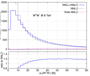
We start by comparing the resummed NNLL+NNLO prediction (blue, solid) for the inclusive $W^{+}W^{-}$ transverse-momentum distribution to the NNLO result (black, dotted) in Fig. 1. As expected, the fixed-order curve diverges at small $p_{T}$ and provides no physical prediction in that region. The resummed result, on the other hand, has a well behaved spectrum down to vanishing transverse momenta. Its spectrum features a kinematical peak at $p_{T}\sim 5$ GeV. At low transverse momenta ($p_{T}\leq 80$ GeV) in Fig. 1 (a), we also study the impact of the finite component (cf. Eq. (3)) to the resummed distribution (magenta, dash-double dotted), which contributes below $1\%$ in the peak region and $\sim 19\%$ at $p_{T}=50$ GeV.

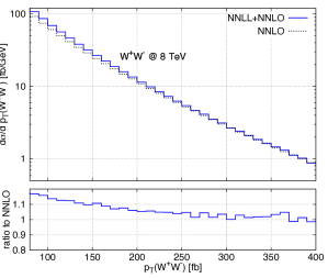
Looking at the ratio of fixed-order and resummed predictions at large transverse momenta ($80$ GeV$\leq p_{T}\leq 400$ GeV) in the lower inset of Fig. 1 (b), we see that the NNLL+NNLO distribution smoothly merges into the NNLO result. We checked that this behaviour is indeed preserved up to very large transverse momenta, which, in fact, renders a hard switching [55] to the fixed-order result feasible. Therefore, the NNLL+NNLO computation provides a uniform prediction which consistently combines low- and high-$p_{T}$ results.

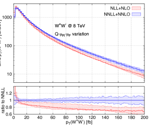
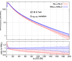
We now turn to our best prediction for $W^{+}W^{-}$ and $ZZ$ transverse-momentum spectra including scale uncertainties that are shown in Figs. 2 (a) and (b), respectively. We compare the resummed NNLL+NNLO result (blue, solid) to NLL+NLO (red, dashed). The uncertainty bands reflect the combined uncertainty from independent $\mu_{F}$, $\mu_{R}$ and $Q$ variations in the ranges $m_{V}\leq\{\mu_{F},\mu_{R}\}\leq 4m_{V}$ and $m_{V}/2\leq Q\leq 2m_{V}$, while constraining $0.5\leq\mu_{F}/\mu_{R}\leq 2$ and $0.5\leq Q/\mu_{R}\leq 2$. By and large we find a consistent reduction of the residual uncertainties: For $W^{+}W^{-}$ the uncertainty at NNLL+NNLO (NLL+NLO) amounts to about $\pm 8\%$ ($\pm 12\%$) at the peak, $\pm 3\%$ ($\pm 5\%$) at $p_{T}=20$ GeV and $\pm 10\%$ ($\pm 15\%$) at $p_{T}=200$ GeV; in case of $ZZ$ the pattern of the uncertainties in the small- and intermediate-$p_{T}$ region is very similar; only at large transverse momenta they are larger than for $W^{+}W^{-}$ reaching up to about $\pm 17\%$ at NNLL+NNLO for $p_{T}=200$ GeV.

The behaviour in the large-$p_{T}$ region is driven by the fixed-order distribution. Let us recall that for $W^{+}W^{-}$ the NNLO corrections [56, 57, 58] for $p_{T}\lesssim 200$ GeV with respect to NLO are quite large ($\sim 40\%)$ and that at least the NLO scale variations underestimate considerably the theoretical uncertainty, given the fact the NLO and NNLO bands do not overlap in that region [16]. Therefore, it is not surprising that we find non-overlapping and hardly-overlapping bands at large transverse momenta for $W^{+}W^{-}$ and $ZZ$, respectively.

3.2 Rapidity dependence of the transverse-momentum spectrum

(a)	(b)

Figure 3: (a) $W^{+}W^{-}$ transverse-momentum shapes at NNLL+NNLO with cuts on the rapidity of the $W^{+}W^{-}$ pair: $|y|<0.5$ (red, solid), $0.5<|y|<1$ (blue, dashed), $1<|y|<2$ (black, dotted), $2<|y|<3$ (magenta, dash-dotted) and $3<|y|$ (orange, double-dash dotted); (b) shape-ratio with respect to the inclusive spectrum.

As described in Section 2 our implementation of the general resummation formalism is fully differential in the $VV^{\prime}$ phase space, i.e., it allows for arbitrary cuts on the kinematics of the $VV^{\prime}$ pair (and even on any of its decay products, once we include the leptonic $VV^{\prime}$ decays by applying the helicity amplitudes of Refs.[59, 60]). A natural double-differential observable concerns the $VV^{\prime}$ $p_{T}$ distribution with an additional cut on the rapidity of the vector-boson pair.

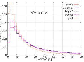
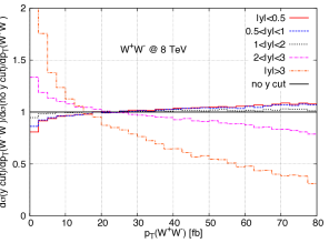
Fig. 3 (a) shows the shape, i.e., normalized such that its integral yields one, of NNLL+NNLO $p_{T}$ distributions of $W^{+}W^{-}$ pairs in various rapidity ranges: $|y|<0.5$ (red, solid), $0.5<|y|<1$ (blue, dashed), $1<|y|<2$ (black, dotted), $2<|y|<3$ (magenta, dash-dotted) and $3<|y|$ (orange, dash-double dotted). In Fig. 3 (b) these curves are normalized to the shape of the inclusive $p_{T}$ distribution. The general observations are the following:

• The $p_{T}$ shapes are hardest at central rapidities and become softer as the rapidity increases.

• In the central region ($|y|<2$) the shape of the $W^{+}W^{-}$ transverse momentum spectrum is rather insensitive to the specific rapidity value. Indeed, the curves become only slightly harder than in the inclusive case.

• In the forward rapidity region the curves feature a significant distortion towards a softer spectrum with respect to the inclusive shape; with deviations of more than a factor of two in the shape-ratio. These effects, however, are strongly phase-space suppressed.

The observed pattern can be understood in the following way: rapidity and transverse momentum are two not completely independent phase-space variables. Indeed, they affect their mutual upper integration bounds. At higher rapidities the kinematically allowed range of transverse momenta is reduced: this squeezes the $p_{T}$ spectrum which consequently becomes softer. This effect has been observed also in previous studies in the case of Higgs boson production [32].

3.3 $p_{T}$-veto efficiencies for $W^{+}W^{-}$ production

Figure 4: $p_{T}$-veto efficiency of the $W^{+}W^{-}$ pair at various orders: NLL+NLO (red, dashed), NNLL+NNLO (blue, solid), NLO (grey, dash-dotted), NNLO (black, dotted), approximate NNLL+NLO (magenta, dash-double dotted); thick lines: central prediction; bands: uncertainty due to combined scale variations; thin lines: borders of bands.

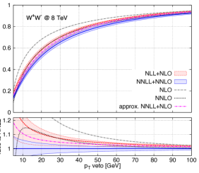
In this section we study efficiencies of the transverse-momentum of the $W^{+}W^{-}$ pair, defined as

$$\epsilon(p_{T}^{\text{veto}})=\sigma(p_{T}<p_{T}^{\text{veto}}{})/\sigma_{\text{tot}}\,,$$ (8)

at various orders in resummed and fixed-order perturbation theory. Fig. 4 shows predictions for $\epsilon(p_{T}^{\text{veto}})$ at the NNLL+NNLO (blue, solid), approximate NNLL+NLO (magenta, dash-double dotted), NLL+NLO (red, dashed), NNLO (black, dotted) and NLO (grey, dash-dotted) as a function of $p_{T}^{\text{veto}}$. In the lower inset the results are normalized to the reference NNLL+NNLO prediction. Approximate NNLL+NLO denotes NLL+NLO, but adding the $g^{(3)}$ function in the Sudakov exponent in Eq. (5), and corresponds to the approximation considered in Refs.[19, 22]. The uncertainty bands involve the independent variations of $\mu_{F}$, $\mu_{R}$ and, where applicable, $Q$, as described in Section 3.1.

The general observation is that both resummation and perturbative higher-order effects yield a sizable reduction of the $p_{T}$-veto efficiency and therefore are vital for a precise theoretical prediction of that quantity. Indeed, the approximated NNLL+NLO result gives some improvement over the NLL+NLO one, but is still roughly $5\%$ above the reference prediction at NNLL+NNLO for $p_{T}^{\text{veto}}\sim 25-30$ GeV. This suggests that the jet-veto efficiency obtained from the reweighting of POWHEG [61] plus Pythia6 [62] with the approximate NNLL+NLO result of the inclusive $W^{+}W^{-}$ $p_{T}$ spectrum in Ref.[22], which was used in the $W^{+}W^{-}$ measurement by CMS [63], might decrease when using the full NNLL+NNLO prediction.

3.4 Comparison to data of the $ZZ$ spectrum

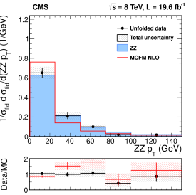
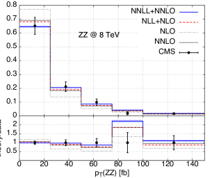
In Fig. 5 we compare the experimental measurement of the $ZZ$ $p_{T}$ distribution by CMS presented in Ref.[17] to predictions at various orders in resummed and fixed-order perturbation theory. Let us stress that the comparison is done at the level of shapes, more precisely the bins add up to one, and that the comparison is not completely consistent, since the experimental $p_{T}$ shape is measured in the fiducial volume, while our predictions are for the fully-inclusive spectrum. Fiducial cuts are not expected to change the picture dramatically though.

That being said, we observe a remarkable agreement between our best NNLL+NNLO prediction (blue, solid curve) and the data points (black dots), except for the single bin ($75$ GeV$\leq p_{T}\leq 100$ GeV) where the experimental uncertainties are largest. Even in this bin the deviation is still below the two sigma level though. We note that also the NNLO (black, dotted) and NLL+NLO (red, dashed) results are in reasonable agreement with the data, the NNLL+NNLO result, however, being always closer to the data points in the low-$p_{T}$ region where resummation effects are relevant; the NLO central prediction (grey, dash-dotted), on the other hand, is quite off in that region.

(a)	(b)

Figure 5: (a) Experimental measurement of the $ZZ$ $p_{T}$ shape in the fiducial region from Ref.[17] and (b) comparison of the data with various predictions at higher orders.

4 Conclusions and outlook

We presented a general implementation of small-$p_{T}$ resummation in the Matrix framework. Logarithmically enhanced contributions are resummed through NNLL accuracy and consistently combined with the NNLO cross section for any process with colorless final states, as long as the respective two-loop amplitude is known.

In this proceedings article we further reviewed the first application of this framework to on-shell $W^{+}W^{-}$ and $ZZ$ production [16], showing results for both the inclusive $p_{T}$ distribution of the pair and within cuts on its momentum. We also reported on results for the $p_{T}$-vetoed cross section and a comparison to experimental data of the $ZZ$ $p_{T}$ spectrum.

Exploiting the helicity amplitudes of Refs.[59, 60] to include the leptonic decays of the vector bosons with off-shell effects and spin correlations as well as the application to further processes is left to future work.

References

- [1] ATLAS Collaboration, Phys.Lett. B716, 1 (2012).
- [2] CMS Collaboration, Phys.Lett. B716, 30 (2012).
- [3] E. Bagnaschi, G. Degrassi, P. Slavich, A. Vicini, JHEP 02, 088 (2012).
- [4] R. V. Harlander, T. Neumann, K. J. Ozeren, M. Wiesemann, JHEP 08, 139 (2012).
- [5] H. Mantler, M. Wiesemann, Eur. Phys. J. C73, 2467 (2013).
- [6] D. de Florian, G. Ferrera, M. Grazzini, D. Tommasini, JHEP 1206, 132 (2012).
- [7] T. Neumann, M. Wiesemann, JHEP 11, 150 (2014).
- [8] R. V. Harlander, H. Mantler, M. Wiesemann, JHEP 11, 116 (2014).
- [9] H. Mantler, M. Wiesemann, Eur. Phys. J. C75, 257 (2015).
- [10] E. Bagnaschi, R. V. Harlander, H. Mantler, A. Vicini, M. Wiesemann, arXiv:1510.08850 (2015).
- [11] A. Banfi, F. Caola, F. A. Dreyer, P. F. Monni, G. P. Salam, G. Zanderighi, F. Dulat (2015).
- [12] S. Kallweit, in preparation.
- [13] S. Catani, M. Grazzini, Phys.Rev.Lett. 98, 222002 (2007).
- [14] M. Grazzini, S. Kallweit, D. Rathlev, M. Wiesemann, in preparation.
- [15] G. Bozzi, S. Catani, D. de Florian, M. Grazzini, Nucl.Phys. B737, 73 (2006).
- [16] M. Grazzini, S. Kallweit, D. Rathlev, M. Wiesemann, JHEP 08, 154 (2015).
- [17] CMS Collaboration, Phys.Lett. B740, 250 (2015).
- [18] C. Balazs, C. Yuan, Phys.Rev. D59, 114007 (1999).
- [19] M. Grazzini, JHEP 0601, 095 (2006).
- [20] R. Frederix, M. Grazzini, Phys.Lett. B662, 353 (2008).
- [21] Y. Wang, C. S. Li, Z. L. Liu, D. Y. Shao, H. T. Li, Phys.Rev. D88, 114017 (2013).
- [22] P. Meade, H. Ramani, M. Zeng, Phys.Rev. D90, 114006 (2014).
- [23] Y. L. Dokshitzer, D. Diakonov, S. Troian, Phys.Lett. B79, 269 (1978).
- [24] G. Parisi, R. Petronzio, Nucl.Phys. B154, 427 (1979).
- [25] G. Curci, M. Greco, Y. Srivastava, Nucl.Phys. B159, 451 (1979).
- [26] J. C. Collins, D. E. Soper, Nucl.Phys. B193, 381 (1981).
- [27] J. Kodaira, L. Trentadue, Phys.Lett. B112, 66 (1982).
- [28] J. Kodaira, L. Trentadue, Phys.Lett. B123, 335 (1983).
- [29] G. Altarelli, R. K. Ellis, M. Greco, G. Martinelli, Nucl.Phys. B246, 12 (1984).
- [30] C. Davies, W. J. Stirling, Nucl.Phys. B244, 337 (1984).
- [31] J. C. Collins, D. E. Soper, G. F. Sterman, Nucl.Phys. B250, 199 (1985).
- [32] G. Bozzi, S. Catani, D. de Florian, M. Grazzini, Nucl.Phys. B791, 1 (2008).
- [33] S. Catani, L. Cieri, D. de Florian, G. Ferrera, M. Grazzini, Nucl.Phys. B881, 414 (2014).
- [34] S. Catani, M. Grazzini, Nucl.Phys. B845, 297 (2011).
- [35] S. Catani, M. Seymour, Nucl.Phys. B485, 291 (1997).
- [36] F. Cascioli, P. Maierhöfer, S. Pozzorini, Phys.Rev.Lett. 108, 111601 (2012).
- [37] A. Denner, S. Dittmaier, L. Hofer, PoS LL2014, 071 (2014).
- [38] A. Denner, S. Dittmaier, Nucl.Phys. B658, 175 (2003).
- [39] A. Denner, S. Dittmaier, Nucl.Phys. B734, 62 (2006).
- [40] A. Denner, S. Dittmaier, Nucl.Phys. B844, 199 (2011).
- [41] G. Ossola, C. G. Papadopoulos, R. Pittau, JHEP 0803, 042 (2008).
- [42] A. van Hameren, Comput.Phys.Commun. 182, 2427 (2011).
- [43] M. Grazzini, S. Kallweit, D. Rathlev, A. Torre, Phys.Lett. B731, 204 (2014).
- [44] F. Cascioli, T. Gehrmann, M. Grazzini, et al., Phys.Lett. B735, 311 (2014).
- [45] T. Gehrmann, M. Grazzini, Kallweit, et al., Phys.Rev.Lett. 113, 212001 (2014).
- [46] M. Grazzini, S. Kallweit, D. Rathlev, JHEP 07, 085 (2015).
- [47] S. Catani, M. Grazzini, Eur.Phys.J. C72, 2013 (2012).
- [48] S. Catani, L. Cieri, D. de Florian, G. Ferrera, M. Grazzini, Eur.Phys.J. C72, 2195 (2012).
- [49] S. Catani, E. D’Emilio, L. Trentadue, Phys.Lett. B211, 335 (1988).
- [50] T. Becher, M. Neubert, Eur.Phys.J. C71, 1665 (2011).
- [51] D. de Florian, M. Grazzini, Phys.Rev.Lett. 85, 4678 (2000).
- [52] D. de Florian, M. Grazzini, Nucl.Phys. B616, 247 (2001).
- [53] S. Catani, D. de Florian, G. Ferrera, M. Grazzini, JHEP 12, 047 (2015).
- [54] R. D. Ball, et al., JHEP 1504, 040 (2015).
- [55] R. V. Harlander, A. Tripathi, M. Wiesemann, Phys.Rev. D90, 015017 (2014).
- [56] S. Dittmaier, S. Kallweit, P. Uwer, Phys.Rev.Lett. 100, 062003 (2008).
- [57] J. M. Campbell, R. K. Ellis, G. Zanderighi, JHEP 0712, 056 (2007).
- [58] S. Dittmaier, S. Kallweit, P. Uwer, Nucl.Phys. B826, 18 (2010).
- [59] F. Caola, J. M. Henn, K. Melnikov, A. V. Smirnov, V. A. Smirnov, JHEP 1506, 129 (2015).
- [60] A. von Manteuffel, L. Tancredi, JHEP 1506, 197 (2015).
- [61] P. Nason, JHEP 0411, 040 (2004).
- [62] T. Sjostrand, S. Mrenna, P. Z. Skands, JHEP 0605, 026 (2006).
- [63] CMS Collaboration, CMS-PAS-SMP-14-016 (2015).