Testing the asymptotic relation for period spacings from mixed modes of red giants observed with the Kepler mission

Abstract

Context. Dipole mixed pulsation modes of consecutive radial order have been detected for thousands of low-mass red-giant stars with the NASA space telescope Kepler. Such modes have the potential to reveal information on the physics of the deep stellar interior.

Aims. Different methods have been proposed to derive an observed value for the gravity-mode period spacing, the most prominent one relying on a relation derived from asymptotic pulsation theory applied to the gravity-mode character of the mixed modes. Our aim is to compare results based on this asymptotic relation with those derived from an empirical approach for three pulsating red-giant stars.

Methods. We developed a data-driven method to perform frequency extraction and mode identification. Next, we used the identified dipole mixed modes to determine the gravity-mode period spacing by means of an empirical method and by means of the asymptotic relation. In our methodology, we consider the phase offset, $\epsilon_{\mathrm{g}}$, of the asymptotic relation as a free parameter.

Results. Using the frequencies of the identified dipole mixed modes for each star in the sample, we derived a value for the gravity-mode period spacing using the two different methods. These differ by less than 5%. The average precision we achieved for the period spacing derived from the asymptotic relation is better than 1%, while that of our data-driven approach is 3%.

Conclusions. Good agreement is found between values for the period spacing derived from the asymptotic relation and from the empirical method. The achieved uncertainties are small, but do not support the ultra-high precision claimed in the literature. The precision from our data-driven method is mostly affected by the differing number of observed dipole mixed modes. For the asymptotic relation, the phase offset $\epsilon_{\mathrm{g}}$ remains ill defined, but enables an more robust analysis of both the asymptotic period spacing and the dimensionless coupling factor. However, its estimation might still offer a valuable observational diagnostic for future theoretical modelling.

1 Introduction

Evolved stars that have exhausted their central hydrogen and are now performing hydrogen burning in a shell surrounding the helium core are generally referred to as red-giant stars or simply red giants (e.g. Cassisi & Salaris, 2013, and references therein). In this work, we will concentrate on red giants with a mass ranging from $\sim$1$\rm M_{\odot}$ up to $\sim$2$\rm M_{\odot}$. These red giants are known to exhibit solar-like oscillations, which are intrinsically damped and stochastically excited by the convective motion of the outer layers of the star (Goldreich & Keeley, 1977; Duvall & Harvey, 1986; Christensen-Dalsgaard et al., 1989; Aerts et al., 2010; Tong & García, 2015).

The seismic analysis of red giants was driven by the photometric observations of space telescopes, such as CoRoT (Baglin et al., 2006; Auvergne et al., 2009) and Kepler (Borucki et al., 2010; Koch et al., 2010). The vast amount of data of unparalleled photometric quality have led to numerous substantial breakthroughs in the asteroseismology of evolved low-mass stars. In particular, a first major leap forward in our seismic understanding of those stars was achieved by Kallinger et al. (2008) and De Ridder et al. (2009) with the detection of non-radial modes in the power-spectral density (PSD) of red giants. This detection allowed for the application of seismic analyses for the measurement of the physical parameters describing the oscillations (Dupret et al., 2009).

Our understanding of red giants drastically improved after the detection of their mixed modes (Beck et al., 2011; Bedding et al., 2011). Such modes contain information from both the deep, dense interior of the star and its convective envelope. Indeed, mixed modes occur due to the coupling between a region in the core where the mode behaves as a gravity (g-) mode and a region in the envelope with pressure (p-)mode behaviour; thus a mixed mode probes conditions both in the core and in the envelope. Exploitation of the detected mixed modes allowed for the discrimination between two evolutionary stages, the red-giant branch (RGB; H-shell burning) and the red clump (RC; He-core and H-shell burning) stars (Bedding et al., 2011; Mosser et al., 2011a), as well as the detection of the rapid core rotation of red giants (Beck et al., 2012; Mosser et al., 2012a).

During its nominal mission, the Kepler space telescope observed more than 15,000 red giants (Huber et al., 2010; Hekker et al., 2011b; Stello et al., 2013; Huber et al., 2014), before a second reaction wheel broke down. In addition, three different star clusters containing red giants were observed, allowing to do ensemble studies (Hekker et al., 2011a; Miglio et al., 2012; Corsaro et al., 2012). Detailed analyses of the oscillation spectrum of individual stars are also being carried out (e.g. di Mauro et al., 2011; Baudin et al., 2012; Deheuvels et al., 2014; Corsaro et al., 2015b, a). Furthermore, the reliability of the seismic tools was tested by studying eclipsing binary stars (Hekker et al., 2010; Frandsen et al., 2013; Gaulme et al., 2013; Beck et al., 2014; Gaulme et al., 2014).

Meanwhile, various approaches to exploit the mixed modes were presented in the literature. The quasi-constant period spacing of mixed modes due to their gravity-mode character allows us to characterise the frequency pattern in the PSD of given stars. This frequency pattern can be calculated using the asymptotic approximation of high-order low-degree gravity modes for a non-rotating evolved star. The asymptotic period spacing for the periods of such consecutive gravity modes with spherical degree $\ell$ is given as:

$$\Delta\Pi_{\ell,\rm asym}=\frac{2\pi^{2}}{\sqrt{\ell(\ell+1)}}\left(\int\limits_{g}\frac{N}{r}\mathrm{d}r\right)^{-1}\ \mathrm{,}$$ (1)

where $N$ is the Brunt-Väisälä frequency and the integration is performed over the g-mode propagation cavity $g$ (Tassoul, 1980; Christensen-Dalsgaard et al., 2011). Such pure gravity modes have high mode inertias and therefore low photometric amplitudes are expected (e.g. Dupret et al., 2009; Grosjean et al., 2014, and references therein).

As a first estimate for the asymptotic period spacing, $\Delta\Pi_{\ell,\rm asym}$, one can use the observed period spacing, $\Delta P$, between mixed modes of the same spherical degree and consecutive radial order to deduce the asymptotic period spacing. Bedding et al. (2011), Mosser et al. (2011a), Corsaro et al. (2012), and Stello et al. (2013) used the average of all observed period spacings between consecutive dipole mixed modes, $\overline{\Delta P}$, to characterise the evolutionary stage of the red giants. However, $\overline{\Delta P}$ is not equal to the quasi-constant asymptotic period spacing caused by the gravity-mode character of the mixed modes and it therefore does not contain the optimal information related to the stellar core.

Mosser et al. (2012b) proposed a formalism, based on the work by Shibahashi (1979) (see also Unno et al., 1989), to describe the full observed frequency pattern of the dipole mixed modes in the oscillation spectrum. This formalism is based on the asymptotic period spacing, $\Delta\Pi_{\ell,\rm asym}$, of pure high radial-order g-modes and the coupling between regions of p- and g-mode behaviour to describe the pattern of the dipole mixed modes. The asymptotic relation for the mixed modes in red giants was recently investigated and verified from detailled stellar and seismic modelling by Jiang & Christensen-Dalsgaard (2014). In addition, alternative approaches have been recently proposed, e.g. by Benomar et al. (2014), relying on the mode inertia to determine the period spacing. The challenge for all methods is to determine the value of the period spacing of the dipole modes with the highest reliability possible.

In this work we intend to evaluate the asymptotic relation introduced by Mosser et al. (2012b) for selected red giants observed by Kepler. Our work is a first step towards the confrontation of the observationally deduced (asymptotic) period spacing with the value calculated from theoretical stellar models tuned to the star under investigation. Here, we limit to the examination whether the high precision of the derived period spacing reported in the literature is supported by our methodology, which covers a large parameter space.

2 Observations and sample

Our analysis is focused on red giants observed with the NASA Kepler space telescope. The giants investigated in this work were selected from visual inspection of thousands of PSDs of the best studied red giants. To be selected, the stars had to fulfil two strict criteria:

• a single clear power-excess, showing pulsations with excellent signal-to-noise ratios (SNRs);

• no visual evidence of rotational splitting in non-radial modes (Gizon & Solanki, 2003; Ballot et al., 2006; Beck et al., 2012; Goupil et al., 2013), since that complicates a direct comparison to frequencies computed with theoretical models.

Using these selection criteria, we identified the three red giants, KIC 6928997, KIC 6762022, and KIC 10593078 as good targets for our analysis. The literature values of the global stellar parameters for these selected stars are presented in Table 1.

The Kepler observations of the three selected red giants were performed in the long cadence mode with a non-equidistant sampling rate of approximately 29.4 min, leading to a Nyquist frequency of $\sim$283.5 $\mu$Hz  (Jenkins et al., 2010). The Kepler dataset covers a time base of 1470 d, leading to a formal frequency resolution of $0.00787$ $\mu$Hz. The Kepler light curves used in this work were extracted from the pixel data for the individual quarters (Q0-Q17) of $\sim$90 days each, following the method described in Bloemen (2013). The final light curve and the power spectral density were compiled and calibrated following the procedure by García et al. (2011). Finally, missing data points up to 20 d were interpolated according to the techniques presented in García et al. (2014) and Pires et al. (2015).

Subsequently, the Kepler light curves were investigated to determine any systematics in the PSDs. Since KIC 6928997 fell on the malfunctioning CCD module in Q5, Q9, and Q13, no observations were obtained during those quarters, leading to slightly stronger side lobes in its spectral window. However, these side lobes were sufficiently weak so that they did not produce significant frequency peaks that would complicate the analysis.

The stars KIC 6928997 and KIC 10593078 have previously been studied by Mosser et al. (2012b, 2014), who reported their asymptotic period spacing, $\Delta\Pi_{\ell,\rm asym}$, and coupling factor, $q$, based on the asymptotic relation. We introduce the asymptotic relation together with $q$ in Sect. 4.2. The values for the asymptotic period spacing are consistent between both studies, but the uncertainties are markedly different: Mosser et al. (2012b) stated $\Delta\Pi_{1,\rm asym}=77.21\pm 0.02$ s with $q=0.14\pm 0.04$, and $\Delta\Pi_{1,\rm asym}=82.11\pm 0.03$ s with $q=0.13\pm 0.04$ for KIC 6928997 and KIC 105930078, respectively, while Mosser et al. (2014) deduced $\Delta\Pi_{1,\rm asym}=77.2\pm 1.4$ s, and $\Delta\Pi_{1,\rm asym}=82.1\pm 1.3$ s. Here, we take a data-driven approach to elaborate on the derivation of those uncertainties.

Table 1: Fundamental parameters for the stars in our sample.

KIC	$K_{\mathrm{p}}$ (mag)	$\mathrm{T_{eff}}$ (K)	$\mathrm{log\ g}$ ($\mathrm{dex}$)	$\mathrm{[Fe/H]}$
6928997	$11.584$	$4800\pm 90$	$2.62$	$0.21$
6762022	$11.532$	$4860\pm 90$	$2.72$	$0.01$
10593078	$11.567$	$4970\pm 100$	$2.88$	$0.17$

3 Frequency analysis

The oscillation properties of solar-like pulsators are usually studied from their PSD diagram. We start our analysis by determining the global shape of the PSD in Sect. 3.1. This allows us to determine the frequency of maximum oscillation power, $\nu_{\rm max}$, defined as the central frequency of the envelope describing the power of the oscillations. Next, we deduce the large frequency separation, $\Delta\nu$, in Sect. 3.2, which describes the equidistant frequency spacing for pure $p$-modes under the asymptotic description (Tassoul, 1980, 1990). It is defined as

$$\Delta\nu=\left(2\int\limits_{0}^{R}\frac{\mathrm{d}r}{c(r)}\right)^{-1}\ \mathrm{,}$$ (2)

where $c(r)$ is the interior sound speed. This parameter is sensitive to the mean stellar density (Ulrich, 1986), while $\nu_{\rm max}$ has been postulated to scale with the surface gravity $g$ and the effective temperature $T_{\mathrm{eff}}$ (Brown et al., 1991; Kjeldsen & Bedding, 1995; Bedding & Kjeldsen, 2003; Belkacem et al., 2011). Therefore, these two quantities depend on the stellar mass and radius and form the basis of the scaling relations broadly used in asteroseismology to derive fundamental stellar properties of solar-like pulsators (i.e. Stello et al., 2008; Gai et al., 2011; Silva Aguirre et al., 2011, 2012; Miglio et al., 2013; Casagrande et al., 2014):

$$\nu_{\mathrm{max}}=\left(\frac{M}{M_{\odot}}\right)\left(\frac{R}{R_{\odot}}\right)^{-2}\left(\frac{T_{\mathrm{eff}}}{T_{\mathrm{eff,\odot}}}\right)^{-0.5}\nu_{\mathrm{max,\odot}}\ \mathrm{,}$$ (3)

and

$$\Delta\nu=\left(\frac{M}{M_{\odot}}\right)^{0.5}\left(\frac{R}{R_{\odot}}\right)^{-1.5}\Delta\nu_{\odot}\ \mathrm{.}$$ (4)

Solar values are indicated by a subscript $\odot$ and we adopt the values of Huber et al. (2011) for $\nu_{\mathrm{max,\odot}}$ and $\Delta\nu_{\odot}$, which are $3150\,\mu$Hz and $134.9\,\mu$Hz, respectively.

In a subsequent step, we extract and identify the individual oscillation modes. To characterise the parameters of each mode in the PSD, we have constructed a semi-automated pipeline. The details on the methods adopted for the extraction and identification of the different modes are presented in Sect. 3.3. The results obtained for the selected sample of red giants are given in Sect. 3.4, and the detailed analysis of the observed dipole mixed modes is further discussed in Sect. 4.

3.1 Determination of the background

The overall shape of the power spectrum of a solar-like oscillator is generally described by a combination of power laws to describe the granulation background signal and a Gaussian envelope to account for the position of the oscillation power excess (e.g. Harvey, 1985; Carrier et al., 2010; Kallinger et al., 2010). The global model of the PSD, expressed as a function of the frequency $\nu$, is given by

$$\mathcal{M}_{\mathrm{PSD}}(\nu)=\left[P_{\mathrm{gran}}(\nu)+P_{\mathrm{Gauss}}(\nu)\right]\cdot R(\nu)+W\ ,$$ (5)

where each term is defined below.

The term corresponding to the granulation signal, $P_{\mathrm{gran}}(\nu)$, is expressed as a sum of $s$ different Lorentzian-like profiles

$$P_{\mathrm{gran}}(\nu)=\sum\limits_{i=1}^{s}\frac{2\pi a_{i}^{2}/b_{i}}{1+\left(\nu/b_{i}\right)^{c_{i}}}\ \mathrm{,}$$ (6)

where each power law is characterised by its amplitude, $a_{i}$, its characteristic frequency, $b_{i}$, and its slope, $c_{i}$. In general two or three different terms are used to describe the granulation contribution, since the granulation activity occurs on different timescales.

Harvey (1985) introducted a Lorentzian profile to describe the granulation signal of the Sun. More recently, Carrier et al. (2010) and Kallinger et al. (2010) found a super-Lorentzian profile (i.e. a Lorentzian with a slope larger than two) to be more appropriate. Kallinger et al. (2014) provided a detailed overview of the determination of the shape of red-giant PSDs and suggested that the description with a slope set to four is favourable. However, in our analysis we choose to keep the slope as a free parameter within the range two to four, to allow more degrees of freedom during the fitting phase for a better fit quality.

The shape of the power excess in the PSD is traditionally described with a Gaussian function

$$P_{\mathrm{Gauss}}(\nu)=P_{g}\exp{\left(-\frac{\left(\nu-\nu_{\mathrm{max}}\right)^{2}}{2\sigma_{g}^{2}}\right)},$$ (7)

while the instrumental noise $W$ in Eq. (5) is assumed to be constant. Aside from the abovementioned contributions to the global model of the PSD, the sampling effects of the dataset need to be considered, since the discretisation of the signal may reduce the power of both the oscillation and the granulation contributions (Karoff et al., 2013; Kallinger et al., 2014). This effect is taken into account by including the response function, $R(\nu)$,

$$R(\nu)=\mathrm{sinc}^{2}\left(\frac{\pi\nu}{2\nu_{\mathrm{Nyq}}}\right)\ \mathrm{,}$$ (8)

where $\nu_{\mathrm{Nyq}}$ is the Nyquist frequency of the Kepler long cadence data.

Estimates of the different parameters describing the background given by Eq. (5) are first obtained by means of a least-squares (LS) minimisation technique. We subsequently refine these estimates by using a Bayesian MCMC (Markov Chain Monte Carlo) algorithm (e.g. Berg, 2004). This technique minimises the following log-likelihood function, $\mathcal{L}(\Theta)$ (Duvall & Harvey, 1986; Anderson et al., 1990),

$$\mathcal{L}(\Theta)=\sum\limits_{k}\left\{\log\left(\mathcal{M}(\Theta;\nu_{k})\right)+\frac{\mathcal{D}(\nu_{k})}{\mathcal{M}(\Theta;\nu_{k})}\right\}\ \mathrm{,}$$ (9)

where $\mathcal{D}(\nu_{k})$ is the data for a certain frequency region $k$ and $\mathcal{M}(\Theta;\nu_{k})$ is the model with the vector parameter $\Theta\leavevmode\nobreak\ =\leavevmode\nobreak\ \left(\Theta_{1},\Theta_{2},\dots,\Theta_{n}\right)$, having $n$ dimensions. The logarithm ensures a high numerical stability. In the current case, the data we wish to describe, $\mathcal{D}$, corresponds to the observed PSD and $\mathcal{M}$ the general shape of the PSD. We use uniform priors for all variables $\Theta_{i}$ defining the model $\mathcal{M}(\Theta;\nu_{k})$, hence we set an upper and lower boundary to each parameter with a uniform probability distribution.

Upon convergence of the Bayesian MCMC routine, the marginal posterior probability distribution is determined for each fitting parameter. We accept the median value of this distribution as the true value for a given parameter in order to capture skewed distributions. Uncertainties on each $\Theta_{i}$ are furthermore extracted from the probability distribution. We present the determined description of the shape of the PSD of KIC 6928997 in Fig. 1 and also indicate the aforementioned individual components.

3.2 Determination of the large frequency separation

In a second step, we deduce the global large frequency separation $\Delta\nu$. To do so, we calculate the autocorrelation function (ACF) of the PSD over a predefined frequency region centred around $\nu_{\rm max}$. The region for the ACF method is defined by using a multiple of the estimate for $\Delta\nu$, which is derived from a scaling relation with the previously derived value of $\nu_{\rm max}$. We use the description by Huber et al. (2010), because it has been calibrated on a large sample of stars. It is given by

$$\Delta\nu_{\mathrm{estimate}}=\left(0.263\pm 0.009\right)\ \nu_{\mathrm{max}}^{0.772\pm 0.005}\ \mathrm{.}$$ (10)

Here, $\Delta\nu_{\mathrm{estimate}}$ represents the estimated value for $\Delta\nu$ through the scaling relation. The frequency region $\nu_{\mathrm{max}}\pm 2\Delta\nu_{\mathrm{estimate}}$ is then passed to the ACF routine to determine a more precise value. We choose to include only this region since we are less sensitive to the variations of $\Delta\nu$ with varying $\nu$ in that way.

Next, we determine the maximum of the ACF in a region around $\Delta\nu_{\mathrm{estimate}}$ and further refine it by fitting a Lorentzian profile. Through this approach, the obtained value for $\Delta\nu$ is not sensitive to the frequency resolution of the ACF. Similar to the PSD model fitting process, the initial estimates on the parameters of the Lorentzian profile are calculated by means of LS minimisation. These are finally passed to the Bayesian MCMC algorithm, again assuming a uniform prior on the fitting parameters and the likelihood function defined in Eq. (9).

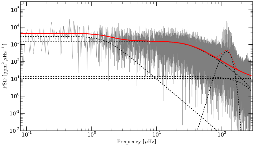
Figure 1: Power density spectrum of the Kepler photometry of KIC 6928997. We represent the individual components describing the background of the PDS by the black dotted lines, their joint effect by the red full line, and the power excess by the red dashed line. Only the solid red line is used as background during the extraction of the oscillations.

3.3 Extraction of the oscillation modes

Once $\nu_{\rm max}$ and $\Delta\nu$ are accurately determined, we extract and identify the individual oscillation modes. We choose to fit the modes one radial-mode order at a time, i.e. we only consider all significant modes between two consecutive radial-mode orders $n_{\mathrm{p}}$ and $n_{\mathrm{p}}+1$, instead of performing a global fit. We define this radial-mode order, $n_{\mathrm{p}}$, as the one of the radial modes and will use it during the mode identification process. It differs from the radial order of the mixed dipole modes, which we call mixed-mode order and denote as $n_{\mathrm{m}}$. The mixed-mode order is dependent upon $n_{\mathrm{p}}$ and upon the radial order of the pure gravity modes, $n_{\mathrm{g}}$ (see e.g. Mosser et al., 2012b). Performing the fitting in a small frequency range leads to fast convergence, since the individual modes are well separated and there are less free parameters compared to fitting the full PSD at once.

A signal-to-noise criterion determines the significance of a given oscillation mode. We calculate this SNR by dividing the PSD by its global shape, Eq. (5), while excluding the Gaussian term, Eq. (7). This general shape corresponds to the solid red line in Fig. 1, while the power-excess is represented by the dashed red line. Mode peaks are considered significant when their SNR is above 7 times the average SNR in the frequency range of that particular radial-mode order.

The profile of solar-like oscillation modes in a PSD is represented by a Lorentzian (Kumar et al., 1988; Anderson et al., 1990), described by

$$P_{\mathrm{mode}}(\nu)=\frac{A^{2}/\pi\Gamma}{1+4\left(\frac{\nu-\nu_{0}}{\Gamma}\right)^{2}}\ \mathrm{,}$$ (11)

where the amplitude, the full width at half maximum (FWHM) and the central frequency of the Lorentzian profile are given by $A$, $\Gamma$, and $\nu_{0}$, respectively. The profile of $k$ significant oscillation modes in a given radial-mode order is then given by

$$\mathcal{M}_{\mathrm{order}}(\nu)=W+R(\nu)\cdot\left[\ P_{\mathrm{gran}}(\nu)+\sum\limits^{k}_{j=1}P_{\mathrm{mode},j}(\nu)\right]\ \mathrm{.}$$ (12)

Both the white noise contribution, $W$, and the granulation contribution, $P_{\mathrm{gran}}(\nu)$, have been determined during the fit to the PSD. Therefore, we keep them fixed during the fitting process per radial-mode order, i.e. only the parameters influencing the individual significant frequencies are varied. Again, we consider the response function, $R(\nu)$, to account for the discrete sampling of the photometric signal.

The developed semi-automated peak-bagging algorithm consists in total of three different steps. First, all significant oscillation modes in a given radial-mode order are fitted with Lorentzian profiles superimposed on the derived background model of the PSD in an automated manner. Second, an interactive fitting step allows the user to have more influence on the fitting process of the individual modes. This is sometimes necessary when the LS minimisation does not converge properly for the very long-lived $g$-dominated mixed modes. Finally, once the initial guesses for the parameters of the fit are sufficient, a Bayesian MCMC algorithm determines the marginal posterior probability distribution for each fitting parameter of an individual mode. The likelihood for the Bayesian fit per radial-mode order is again described by Eq. (9). We adopt uniform priors for both the central frequency and the amplitude of a given peak, while a modified Jeffreys’ prior (Handberg & Campante, 2011) is used for the FWHM of the Lorentzian profiles.

The mode identification was performed for the retrieved peaks by using a dimensionless reduced phase shift $\theta$ defined from a frequency échelle diagram as

$$\theta=\left(\nu/\Delta\nu\right)-\left(n_{\mathrm{p}}+\epsilon\right)$$ (13)

and having a value in the interval $-0.2\leq\theta<0.8$. Here, $\nu$ and $n_{\mathrm{p}}$ are the frequency and the radial-mode order, respectively, and $\epsilon$ is a small constant that occurs from an asymptotic approximation for the mode frequencies. This constant can be approximated using the scaling relation presented in Mosser et al. (2011b), and updated by Corsaro et al. (2012), which leads to radial modes having $\theta\approx 0.00$ and quadrupole modes having $\theta\approx-0.12$ (see also Tassoul, 1980; Mosser et al., 2012a). Dipole p-modes, on the other hand, have $0.2\leq\theta<0.8$ and $\ell=3$ modes have $0.1<\theta<0.2$. We choose to estimate $\epsilon$ for each radial-mode order from the radial modes assuming their $\theta$ to be exactly zero and approximating $n_{\mathrm{p}}$ as $\lfloor\nu_{\ell=0}/\Delta\nu\rfloor-1$, instead of using the empirical scaling relation.

3.4 Results

The derived values for the global asteroseismic properties $\nu_{\rm max}$ and $\Delta\nu$ obtained by using the Bayesian MCMC methods are presented in Table 2, including their $1\sigma$ uncertainties corresponding with an 68% probability that the true value is included in the overall interval.

Table 2: Determined seismic parameters of the stars in our sample.

KIC	$\nu_{\mathrm{max}}$ ($\mathrm{\mu Hz}$)	$\Delta\nu$ ($\mathrm{\mu Hz}$)
6928997	$119.13^{+0.39}_{-0.35}$	$10.015_{-0.005}^{+0.005}$
6762022	$41.02^{+0.18}_{-0.22}$	$4.455_{-0.009}^{+0.010}$
10593078	$206.98^{+0.25}_{-0.34}$	$15.428^{+0.019}_{-0.020}$

We find significant oscillation modes in regions in-between six consecutive radial modes, corresponding to five different radial-mode orders $n_{\mathrm{p}}$. Therefore, we consistently restrict the analysis at most to the central five radial-mode orders throughout this work. Additional care is taken to only obtain frequencies that could unambiguously be identified, i.e. no dipole mode was considered outside the expected region. Although other work often takes such modes into account, increasing the total number of frequencies available, we choose to reject them. For KIC 6762022, significant dipole modes only occurred in its three central radial-mode regions so we restricted to this regime for this star.

4 Period spacing analysis

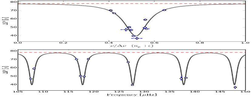
Figure 2: Derivation of $\Delta\Pi_{1,\rm emp}$ for KIC 6928997 using the empirical approach of fitting $\Delta P$, yielding $\Delta\Pi_{1,\rm emp}=81.14\ \mathrm{s}$ (red dashed). The fit is done for the phase shift $\theta$ (top) and subsequently expanded to $\nu$ (bottom), using the inverse relation of Eq. (13).

The dipole mixed modes in evolved stars take on an acoustic-mode nature in the outer envelope and a gravity-mode nature in the deep interior (Dziembowski et al., 2001; Christensen-Dalsgaard, 2004; Dupret et al., 2009; Montalbán et al., 2010). This causes their period spacing to deviate from the constant value expected for pure $g$-modes in the asymptotic approximation. The dipole mixed modes turn out to be detectable at the stellar surface by means of high precision photometry (Beck et al., 2011; Bedding et al., 2011; Mosser et al., 2011a).

The period difference (expressed in seconds) between two consecutive dipole mixed modes is formally named the observed period spacing and is defined as

$$\Delta P=\frac{1}{\nu_{n_{\mathrm{m}}}}-\frac{1}{\nu_{n_{\mathrm{m}}+1}}\,.$$ (14)

The average of all observed period spacings, $\overline{\Delta P}$ is a good indicator of the evolutionary stage of a given star (e.g. Bedding et al., 2011; Mosser et al., 2011a; Corsaro et al., 2012) and is reported in Table 3.

The observed period spacing measured from consecutive mixed modes, $\Delta P$, can be used to infer the value of the asymptotic period spacing of dipole mixed modes $\Delta\Pi_{1}$, which is given analytically by Eq. (1) for any spherical degree $\ell>0$. Here, we test two different methods to derive $\Delta\Pi_{1}$ and explore their reliability, without considering frequency-dependent variations of $\Delta\Pi_{1}$ caused by structural glitches in the core of the star (Cunha et al., 2015).

4.1 Lorentzian fitting to $\Delta P$

To obtain a first estimate for the value of the asymptotic period spacing $\Delta\Pi_{1}$ for a given red-giant star, we use an empirical approach (see Stello, 2012). This approach captures the mixed character due to the pressure and the gravity nature of the dipole modes seen in the observed period spacings, $\Delta P$, related to the mode bumping (Deheuvels & Michel, 2010). When mixed modes show a very strong gravity character, $\Delta P$ remains fairly constant and close to the value of $\Delta\Pi_{1}$. However, when the character of the mixed modes becomes more pressure-like, a lower $\Delta P$ is expected and observed. Thus, the behaviour of the mixed modes can be captured by a convolution of a flat continuum, accounting for $\Delta\Pi_{1}$ in case of pure $g$-modes, and a Lorentzian profile with negative height, taking the mixed mode nature into account by reducing the strength of the $g$-mode character of the mixed modes.

We choose again to work with the previously defined dimensionless reduced phase shift $\theta$, since it allows for a more stable fitting procedure. An average phase shift

$$\theta_{\rm spacing}=\frac{\theta_{n_{\mathrm{m}}}+\theta_{n_{\mathrm{m}}+1}}{2}\ \mathrm{,}$$ (15)

is assigned for each observed period spacing $\Delta P$. This enables us to describe the profile for the mixed mode period spacings as:

$$\mathcal{M}_{\rm emp}(\theta_{\rm spacing})=\Delta\Pi_{\rm emp}-\frac{H}{1+4\left(\frac{\theta_{\rm spacing}-\theta_{0}}{\Gamma}\right)^{2}}\ \mathrm{,}$$ (16)

where $H$ is the height of the Lorentzian profile centred at $\theta_{0}$ with a width $\Gamma$. A LS minimisation technique is adopted to perform the process of fitting $\mathcal{M}_{\rm emp}$ to the observed period spacings in terms of the parameters $\Delta\Pi_{\rm emp}$, $H$, $\Gamma$, and $\theta_{0}$. Estimates on the uncertainties on the individual free parameters are deduced by means of a Monte Carlo approach. We randomly perturb the extracted the extracted dipole frequencies 25,000 times within their respective uncertainties and determine their $\Delta P$ and $\theta_{\rm spacing}$. For the perturbation, we assume normally distributed errors. The fitting process is repeated on each iteration and the scatter on the final set of fitting parameters is then an indication on their uncertainties. The results for this method are reported for the three stars in Table 3 as the empirical values $\Delta\Pi_{1,\rm emp}$.

4.2 Exploration of the asymptotic relation

Mosser et al. (2012b) proposed to derive $\Delta\Pi_{1}$ by solving the equations of Shibahashi (1979) and formulated the approximation for a frequency of a dipole mode $\nu_{\rm m}$ as

$$\nu_{\rm m}=\nu_{\mathrm{n_{p}},\ell=1}+\frac{\Delta\nu}{\pi}\mathrm{arctan}\left[q\ \mathrm{tan}\,\pi\left(\frac{1}{\Delta\Pi_{1,\rm asym}\nu_{\rm m}}-\epsilon_{\mathrm{g}}\right)\right]\ \mathrm{.}$$ (17)

The frequencies of the gravity modes are coupled to the frequency of the pure $p$-mode $\nu_{\mathrm{n_{p}}}$. The dimensionless coupling factor $q$ describes the strength of the coupling between the gravity mode cavity and the pressure mode region. It typically has a value between $0.1$ and $0.3$ (Mosser et al., 2012b). The constant $\epsilon_{\mathrm{g}}$ is a phase offset that ensures a proper behaviour for the g-mode periods in the case of weak coupling. Mosser et al. (2012b) assumed this constant to be zero. Here, we explore the possibility of varying this phase offset rather than keeping it constant.

Because the asymptotic relation is an implicit equation for $\nu_{\rm m}$, we solve Eq. (17) by means of a geometrical technique, oversampling the observed frequency resolution a 1000 times, as described by Beck (2013). Second-order asymptotics are considered for the pure pressure modes. Different approaches have been proposed to derive $\Delta\Pi_{1,\rm asym}$ with the asymptotic relation from observations. Typically, a LS minimisation with an initial guess close to the expected value of $\Delta\Pi_{1,\rm asym}$ is used to search in a narrow range of solutions (e.g. Mosser et al., 2012b, 2014).

Our aim is to investigate in depth the solution of $\Delta\Pi_{1}$, using the asymptotic relation, by exploring a tri-dimensional parameter space for ($\Delta\Pi_{1,\rm asym}$, $q$, $\epsilon_{\mathrm{g}}$), thus allowing us to understand the reliability of the final estimate of the asymptotic dipole period spacing. This is accomplished by means of a grid-search method, where we vary the parameters $\Delta\Pi_{1}$ and $q$ over a wide range of values, while $\epsilon_{\mathrm{g}}$ is varied between 0 and 1. As far as we are aware, it is the first time that the phase offset, $\epsilon_{\mathrm{g}}$, of the asymptotic relation is considered a free parameter.

The fit quality for a combination of values of ($\Delta\Pi_{1,\rm asym}$, $q$, $\epsilon_{\mathrm{g}}$) is quantified by means of a $\chi^{2}$ test, where we compute the difference between the predicted asymptotic frequencies and those observed. The adopted $\chi^{2}$ is defined as

$$\chi^{2}_{\mathrm{grid}}(\Delta\Pi_{1},\,q,\,\epsilon_{\mathrm{g}})=\frac{1}{N-4}\sum\limits^{N}_{i}\left(\frac{\nu_{\ell=1,i,\mathrm{obs}}-\nu_{\ell=1,i,\mathrm{asym}}}{\sigma(\nu_{\ell=1,i,\mathrm{obs}})}\right)^{2}\ \mathrm{,}$$ (18)

where $\nu_{\ell=1,i,\mathrm{obs}}$ is the frequency of the $i$-th observed dipole mixed mode and $\sigma(\nu_{\ell=1,i,\mathrm{obs}})$ its corresponding standard deviation estimated by the Bayesian MCMC fit. The related frequency from the asymptotic relation, the closest one to the $i$-th observed mixed mode $\nu_{\ell=1,i,\mathrm{asympt}}$, is calculated following Beck (2013) and $\chi^{2}_{\mathrm{grid}}$ is normalised by $N-4$ degrees of freedom, where $N$ is the number of observed dipole mixed modes for a given red-giant star.

The value of $\Delta\Pi_{1,\rm emp}$, determined in Sect. 4.1, acts as a starting point for the $\Delta\Pi_{1,\rm asym}$ axis in the tri-dimensional parameter space analysis. We let this parameter vary up to $\pm 10\%$ of the initial guess $\Delta\Pi_{1,\rm emp}$, and sample with a resolution of 0.02 s (0.04 s for RC stars). Solutions with a coupling factor $q$ ranging from 0.01 up to 0.51, with a resolution of 0.005, were considered. The phase offset $\epsilon_{\mathrm{g}}$ spanned from 0 to 1, with a step of 0.0025, noting that any values smaller than zero or larger than one will behave similarly as those in the used range due to the periodicity of the tangent function. As such, we construct a grid of several millions of points, with dimension (500,100,400), each grid point representing a unique combination of ($\Delta\Pi_{1,\rm asym}$, $q$, $\epsilon_{\mathrm{g}}$). At each meshpoint, we compare the calculated frequencies using the asymptotic relation with those extracted from the PSD to obtain the most probable solution. This best set of values for $\Delta\Pi_{1,\rm asym}$, $q$, and $\epsilon_{\mathrm{g}}$ is reported in Table 3.

To study each dimension in our tri-dimensional parameter space in more detail, we use marginal distributions. In practice, we consider a minimum $\chi^{2}_{\mathrm{grid}}$ per gridpoint along one dimension to reduce the dimensionality and by marginalising over this dimension we assess the correlation between the two remaining dimensions. Applying this technique over two dimensions enables us to construct confidence intervals for the third, remaining dimension, since it represents the distribution of that dimension, similar to the computation of the marginal posterior probability in a Bayesian MCMC analysis.

We construct the confidence intervals by relying on the theory of $\chi^{2}$ statistics using $\chi^{2}$ tests, i.e. the $\chi^{2}_{\alpha}$ value for an $\alpha\,\%$ confidence interval. This $\chi^{2}_{\alpha}$ level corresponds to a $\chi^{2}_{\mathrm{grid}}$ value indicating the found $\chi^{2}_{\mathrm{grid}}$ minimum is the real minimum with an $\alpha\,\%$ certainty and is computed as

$$\chi^{2}_{\alpha}=\frac{\chi^{2}_{\alpha,k}\ \cdot\chi^{2}_{\mathrm{grid,\ min}}}{k}\ \mathrm{,}$$ (19)

with $k=N-4$ degrees of freedom, $\chi^{2}_{\mathrm{grid,\ min}}$ the value for the optimal solution, and $\chi^{2}_{\alpha,k}$ the tabulated value for an $\alpha\,\%$ inclusion of the cumulative distribution function of a $\chi^{2}$ distribution with $k$ degrees of freedom. We divide by the degrees of freedom, since the $\chi^{2}$ test in Eq. (18) contains a sum of multiple distributions. The multiplication by $\chi^{2}_{\mathrm{min}}$ accounts for the difference between the optimal value and the expected value of 1. The parameter ranges in the 1D marginal distributions are then taken as the confidence interval for that parameter.

4.3 Results

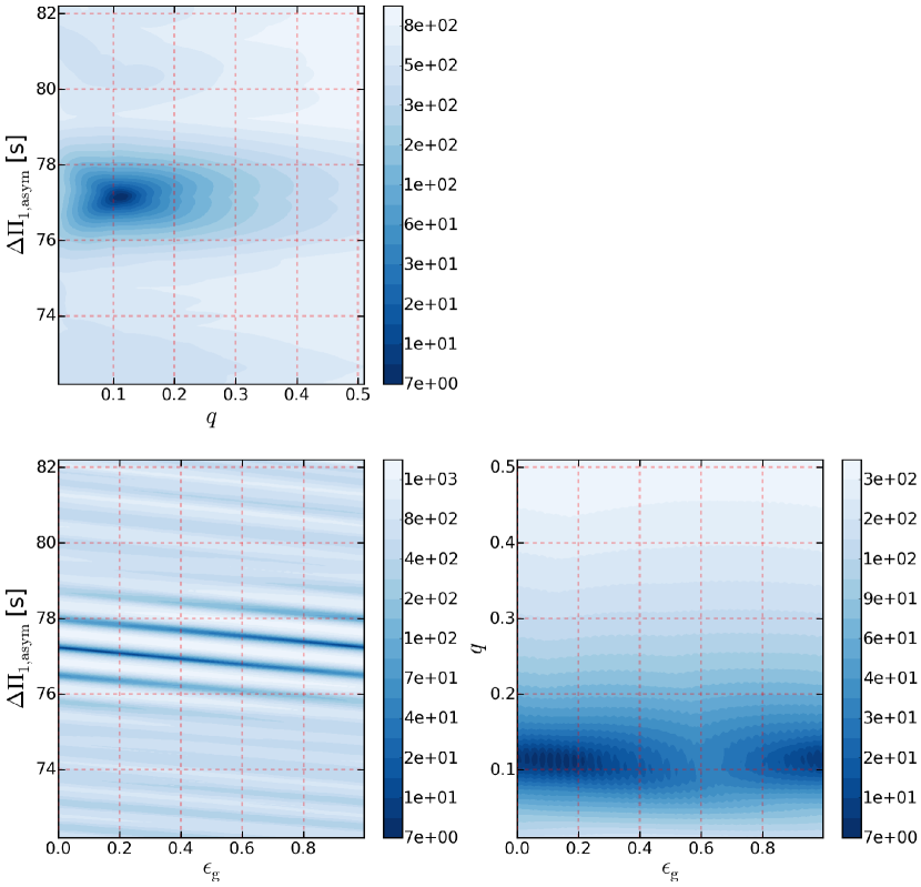
Figure 3: Correlation maps indicating the $\chi^{2}_{\mathrm{grid}}$ as a colour map for KIC 6928997, as deduced from the asymptotic relation Eq. (17). The one-dimensional marginal distributions are given in Fig. 11. The $\chi^{2}_{\mathrm{grid}}$ levels are indicated by the various colourbars. Top left: Correlation map of the marginal bi-dimensional parameter space ($\Delta\Pi_{1,\rm asym}$, $q$). The darkest shade indicates the most likely solution. Bottom left: Correlation map of the the marginal bi-dimensional parameter space ($\Delta\Pi_{1,\rm asym}$, $\epsilon_{\mathrm{g}}$). A strong correlation is observed between both parameters. Bottom right: Correlation map of the the marginal bi-dimensional parameter space ($q$, $\epsilon_{\mathrm{g}}$). Correlation maps for the two other stars in our sample are given in the Appendix.

Figure 2 illustrates that the Lorentzian profile captures the mixed nature of the dipole modes reasonably well for KIC 6928997. As such, the value of $\Delta\Pi_{1,\rm emp}$ can be used as a better starting point, compared to $\overline{\Delta P}$, for the more elaborate tri-dimensional parameter search. From the Monte Carlo analysis we were able to determine the uncertainties for $\Delta\Pi_{1,\rm emp}$, which had a Gaussian-like distribution for both KIC 6928997 and KIC 10593078. For KIC 6762022, however, the profile indicated a bi-modal distribution, leading to a much larger uncertainty on $\Delta\Pi_{1,\rm emp}$. This is caused by a strongly gravity-dominated mixed dipole mode. Performing perturbations of the two corresponding frequencies will often give a $\Delta P$ value larger than the optimal $\Delta\Pi_{1,\rm emp}$, producing the bi-modality of the Monte Carlo distribution.

Figures 3 and 5 show the different marginal distributions for the mixed modes derived from the asymptotic relation for KIC 692897 (the same figures are given in the Appendix for the two remaining red giants of the sample) . We accept the $\Delta\Pi_{1,\rm asym}$ values derived with this method as our final values for $\Delta\Pi_{1}$. Studying the different marginal distributions enabled use to discuss the behaviour of the asymptotic relation in more detail.

The correlation maps show that there is a significant correlation between $\Delta\Pi_{1,\rm asym}$ and the phase offset $\epsilon_{\mathrm{g}}$ (bottom left panel Fig. 3). This was anticipated from looking at Eq. (17), since both parameters are present within the tangent-function. As such, it is possible to have the same mixed-mode frequencies for various $\Delta\Pi_{1,\rm asym}$ combined with appropriate $\epsilon_{\mathrm{g}}$ values. Also, fixing $\epsilon_{\mathrm{g}}$ to one unique value prohibits capturing the complete behaviour of the asymptotic relation. This is shown in Fig. 4, where we indicate the correlation map between $\Delta\Pi_{1,\rm asym}$ and $q$, assuming $\epsilon_{\mathrm{g}}=0$. Since the phase offset is assumed to be constant, the frequency space of the mixed modes is not fully sampled. Thus, the colour map mimics a correlation between $\Delta\Pi_{1,\rm asym}$ and $q$ and produces a multi-modal behaviour in the marginal $\Delta\Pi_{1,\rm asym}$ distribution. No other significant correlations are observed between the other parameters in the tri-dimensional parameter space nor between the coupling factor, $q$, and the value of the tangent term within the asymptotic relation, Eq. (17). However, the marginal distribution of $\epsilon_{\mathrm{g}}$ is sensitive to the sampling rate along the $\Delta\Pi_{1,\rm asym}$ axis. The larger the difference between consecutive $\Delta\Pi_{1,\rm asym}$ values, the stronger the wiggles are in the bottom panel of Fig. 5. These wiggles are understood as the influence of the correlation between $\Delta\Pi_{1,\rm asym}$ and $\epsilon_{\mathrm{g}}$ on the chosen sampling rates. Indeed, performing a first order perturbation analysis of Eq. 17, assuming a constant $q$ and $\nu_{\rm m}$, leads to the relation

$$\delta(\epsilon_{\mathrm{g}})=\left|\frac{\delta(\Delta\Pi_{1,\rm asym})}{\Delta\Pi_{1,\rm asym}^{2}\nu_{\rm m}}\right|\ \mathrm{,}$$ (20)

where $\delta(\epsilon_{\mathrm{g}})$ and $\delta(\Delta\Pi_{1,\rm asym})$ are the perturbations on $\epsilon_{\mathrm{g}}$ and $\Delta\Pi_{1,\rm asym}$, respectively. Considering $\delta(\Delta\Pi_{1,\rm asym})$ as our chosen sampling rate of $\Delta\Pi_{1,\rm asym}$ indicates that we inherently sample our $\epsilon_{\mathrm{g}}$ axis. Using the accepted $\Delta\Pi_{1,\rm asym}$, approximating $\nu_{\rm m}$ as $\nu_{\rm max}$, and taking the chosen sampling rate $\delta(\Delta\Pi_{1,\rm asym})=0.02$ s for KIC 6928997 results in a $\delta(\epsilon_{\mathrm{g}})=0.028$, which is similar to the size of the wiggles observed in the bottom panel of Fig. 5. A smaller sampling rate along $\Delta\Pi_{1,\rm asym}$ would provide a smoother marginal profile at a computational expense. However, it would be unlikely that this smoother distribution behaves substantially different.

Second, the inclusion of the phase offset $\epsilon_{\mathrm{g}}$ as a variable parameter permitted us to determine correct confidence interval for each parameter. Both $\Delta\Pi_{1,\rm asym}$ and $q$ are strongly confined, unlike $\epsilon_{\mathrm{g}}$. The confidence interval for $\epsilon_{\mathrm{g}}$ spans a large portion of the parameter space. We mark the boundaries for the various confidence intervals in Fig. 5. Nevertheless, the inclusion of the phase offset is mandatory if one wants to study $\Delta\Pi_{1,\rm asym}$ in detail, due the above-mentioned correlation. In the present analysis, $\epsilon_{\mathrm{g}}$ does not in itself provide very useful information, owing to its large confidence interval, but must be accounted for in the study of the parameters which are of interest, $\Delta\Pi_{1,\rm asym}$ and $q$. Despite this behaviour of $\epsilon_{\mathrm{g}}$, we did not lose any information, since $\epsilon_{\mathrm{g}}$ was artificially set to zero in previous studies, but did gain more understanding of $\Delta\Pi_{1,\rm asym}$.

Lastly, we note that the marginal distribution of $\Delta\Pi_{1,\rm asym}$ looks significantly different for both KIC 6762022 and KIC 10593078 compared to KIC 6928997 (see figures in Appendix). The distributions of the former show a different shape around the minimum $\chi^{2}_{\mathrm{grid}}$ value, resembling a local and a global minimum. A possible explanation is the presence of buoyancy glitches, giving rise to slightly different $\Delta\Pi_{1,\rm asym}$ values for different radial-mode orders. A detailed study of the dipole mixed-mode frequencies per radial-mode order is of interest, but is out of the scope of the current work.

We construct frequency and period échelle diagrams (such as Fig. 6) for further visual comparison between the frequencies of the dipole mixed modes extracted from the PSD and those calculated with the asymptotic relation $\nu_{\rm m}$. Only very small differences between the extracted dipole mixed modes and the corresponding $\nu_{\rm m}$ are seen in the frequency échelle diagram. In addition, the period échelle spectrum captures the behaviour of the mixed modes very well, confirming that the extracted modes indeed show a mixed behaviour, making the asymptotic relation appropriate.

Differences between values for $\Delta\Pi_{1}$ derived by the two methods are slightly larger than the uncertainties and more pronounced for the confidence intervals of $\Delta\Pi_{1}$ themselves. Uncertainties determined from the tri-dimensional parameter space are significantly smaller. In addition, the asymptotic relation provides information related to the strength of the coupling between the different propagation zones and a slight hint for the phase offset required for asymptotic theory. Our results determined by means of the asymptotic relation agree with those in the literature, yet are slightly different since we considered $\epsilon_{\mathrm{g}}$ to be a free parameter. The major contrast is witnessed for the uncertainties for $\Delta\Pi_{1,\rm asym}$. They range between those proposed by Mosser et al. (2012b) and Mosser et al. (2014) and are asymmetric.

Table 3: Results for the period spacing determined from the extracted dipole frequencies of Q0-Q17 Kepler data.

KIC	$\overline{\Delta P}$	Evolutionary	$\Delta\Pi_{1,\rm emp}$	$\Delta\Pi_{1,\rm asym}$	$q$	$\epsilon_{\mathrm{g}}$
		state	Empirical	Asymptotic
	[s]	[s]	[s]	[s]	[ ]	[ ]
6928997	$53.1\pm 11.2$	RGB	$78.3_{-3.3}^{+4.2}$	$77.10_{-0.13}^{+0.22}$	$0.111^{+0.023}_{-0.018}$	$0.160_{-0.271}^{+0.165}$
6762022	$210.3\pm 19.1$	RC	$261.9_{-18.4}^{+25.9\leavevmode\nobreak\ a}$	$259.08_{-1.63}^{+1.19}$	$0.240^{+0.091}_{-0.063}$	$0.835_{-0.420}^{+0.580}$
10593078	$53.7\pm 14.3$	RGB	$81.8_{-1.0}^{+1.2}$	$82.48_{-0.83}^{+0.47}$	$0.130^{+0.073}_{-0.054}$	$0.755_{-0.326}^{+0.608}$

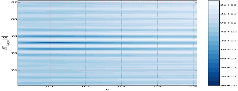
Figure 4: Correlation maps indicating the $\chi^{2}_{\mathrm{grid}}$ as a colour map for KIC 6928997, as deduced from the asymptotic relation Eq. (17) and assuming $\epsilon_{\mathrm{g}}$ is fixed at zero.

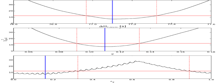
Figure 5: One dimensional marginal distributions for each parameter considered in the asymptotic relation for KIC 6928997, centred on the optimal solution, which is marked in blue. The $\chi^{2}_{\mathrm{95\%}}$ value is marked by the solid red line. The upper (lower) boundaries for the uncertainty on the individual parameters are given by the red dotted lines. The marginal distribution for each parameter over the full tri-dimensional grid is given in Fig. 11 in the Appendix.

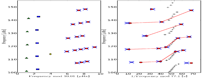
Figure 6: Échelle diagrams comparing the solution of the asymptotic relation ($\Delta\Pi_{1,\rm asym}=77.1\ \mathrm{s}$, $q=0.11$ and $\epsilon_{\mathrm{g}}=0.16$) with extracted modes for KIC 6928997. Left: a frequency échelle diagram, comparing the frequencies of the asymptotic relation to those from the mode extraction. The extracted radial, dipole, quadrupole and octupole modes are indicated by blue squares, red dots, green triangles, and yellow diamonds, respectively. The frequencies of the dipole mixed modes obtained from the asymptotic relation, and having an observational counterpart, are indicated by blue crosses. Right: a period échelle spectrum for the dipole modes, showing the same comparison as in the left panel with the same colour coding. The black ’+’ indicate the frequencies for the mixed modes obtained from the asymptotic relation without any observational counterparts.

5 Conclusions

In this work, we analysed the dipole mixed mode period spacing of three red giants observed by the NASA Kepler space telescope. Two of them are in the evolutionary stage of hydrogen shell burning, while the third one was confirmed to be in the more advanced helium core-burning phase. We determine the value for $\Delta\Pi_{1}$, the g-mode asymptotic period spacing, according to two different approaches. First, we used an empirical fit to the observed period spacings. Next, the description of the asymptotic relation is used to study the tri-dimensional parameter space of $\Delta\Pi_{1,\rm asym}$, $q$, and $\epsilon_{\mathrm{g}}$. We were able to determine realistic confidence intervals for both the asymptotic period spacing and the dimensionless coupling factor. The phase offset $\epsilon_{\mathrm{g}}$, however, remains ill defined due its large confidence interval. Yet, it is only by considering $\epsilon_{\mathrm{g}}$ as a variable parameter and using marginal distributions that the determination of a confidence interval for the asymptotic period spacing is simplified, because a fixed $\epsilon_{\mathrm{g}}$ provides a multi-modal behaviour in the $\chi^{2}$ landscape.

The two approaches have very different computational efficiencies, but lead to compatible results. Our conclusion is that, when analysing large samples of stars, particular attention has to be given to the techniques adopted to estimate the value of $\Delta\Pi_{1}$ and meaningful uncertainties are needed in order to be able to perform a reliable comparison between observations and stellar models. The results obtained in this work, allowing for a varying $\epsilon_{\rm g}$, provide reliable uncertainty estimates, which are in between those quoted by Mosser et al. (2012b) and Mosser et al. (2014), i.e. meaningful estimates of the relative uncertainty of the period spacing range up to 1 %.

Determining the period spacing per radial-mode order constitutes a next step onwards, since the marginal distribution of $\Delta\Pi_{1,\rm asym}$ indicated a substructure around the optimal solution. This would provide information about possible structural glitches in the core, which were ignored in this work. However, this is only possible if enough dipole mixed modes are identified per radial-mode order. Another possibility is to include the large frequency separation as a fourth parameter in the study of the asymptotic relation. At present, we fixed this value since it was deduced with a very high accuracy during the detailed frequency analysis.

Appendix A Marginal distributions

Here, we present the various marginal distributions for the two remaining red giants, KIC 6762022 and KIC 10593078. They are similar to the figures presented in Sect. 4.3. In addition, we provide the 1D marginal distributions over the full tri-dimensional grid for each parameter and for each star.

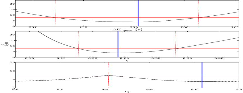
Figure 7: One dimensional marginal distributions for each parameter considered in the asymptotic relation for KIC 6762022, centred at the optimal solution. Similar figure as Fig. 5.

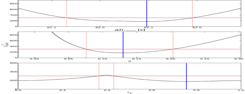
Figure 8: One dimensional marginal distributions for each parameter considered in the asymptotic relation for KIC 10593078, centred at the optimal solution. Similar figure as Fig. 5.

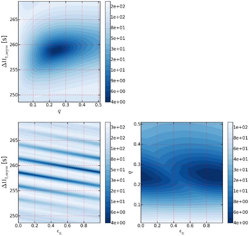
Figure 9: Correlation maps indicating the $\chi^{2}_{\mathrm{grid}}$ as a colour map for KIC 6762022, as deduced with the asymptotic relation Eq. (17). Similar figure as Fig. 3.

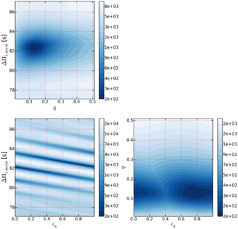
Figure 10: Correlation maps indicating the $\chi^{2}_{\mathrm{grid}}$ as a colour map for KIC 10593078, as deduced with the asymptotic relation Eq. (17). Similar figure as Fig. 3.

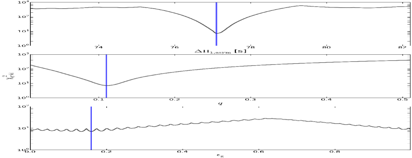
Figure 11: One dimensional marginal distributions for each parameter considered in the asymptotic relation for KIC 6928997. The final values for each parameter, corresponding to the best description for the dipole mixed modes with the asymptotic relation are marked in blue.

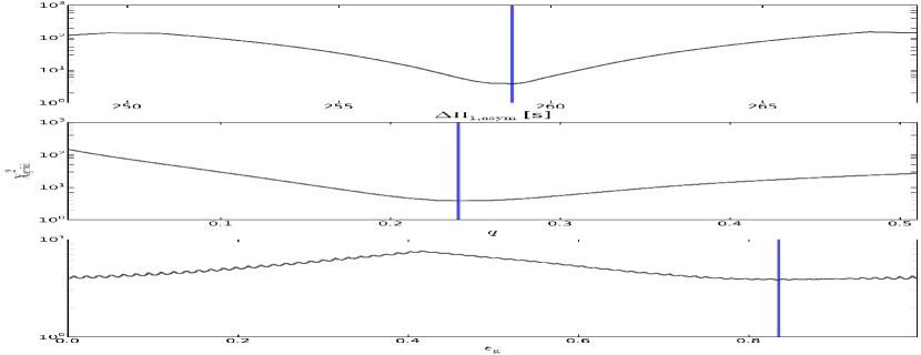
Figure 12: One dimensional marginal distributions for each parameter considered in the asymptotic relation for KIC 6762022. Similar figure as Fig. 11.

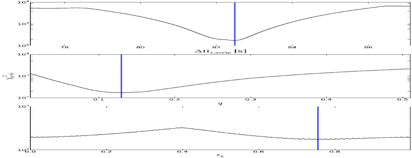
Figure 13: One dimensional marginal distributions for each parameter considered in the asymptotic relation for KIC 10593078. Similar figure as Fig. 11.