Inclusive jet spectrum for small-radius jets

Abstract

Following on our earlier work on leading-logarithmic (LL_R) resummations for the properties of jets with a small radius, $R$, we here examine the phenomenological considerations for the inclusive jet spectrum. We discuss how to match the NLO predictions with small-$R$ resummation. As part of the study we propose a new, physically-inspired prescription for fixed-order predictions and their uncertainties. We investigate the $R$-dependent part of the next-to-next-to-leading order (NNLO) corrections, which is found to be substantial, and comment on the implications for scale choices in inclusive jet calculations. We also examine hadronisation corrections, identifying potential limitations of earlier analytical work with regards to their $p_{t}$-dependence. Finally we assemble these different elements in order to compare matched (N)NLO+LL_R predictions to data from ALICE and ATLAS, finding improved consistency for the $R$-dependence of the results relative to NLO predictions.

1 Introduction

Jets are used in a broad range of physics analyses at colliders and notably at CERN’s large hadron collider (LHC). The study of jets requires the use of a jet definition and for many of the algorithms in use today that jet definition involves a “radius” parameter, $R$, which determines how far in angle a jet clusters radiation. A limit of particular interest is that where $R$ is taken small. One reason is that contamination from multiple simultaneous $pp$ interactions (“pileup”) is minimised, as is the contribution from the large underlying event when studying heavy-ion collisions. Furthermore small-$R$ subjets are often a component of jet substructure analyses used to reconstruct hadronic decays of highly boosted weak bosons and top quarks. Finally a powerful systematic cross-check in precision jet studies comes from the variation of $R$, e.g. to verify that conclusions about data–theory agreement remain stable. Such a variation will often bring one into the small-$R$ limit.

In the small-$R$ limit the perturbative series involves terms $\alpha_{s}^{n}\ln^{n}1/R^{2}$, where the smallness of $\alpha_{s}^{n}$ is partially compensated by large logarithms $\ln^{n}1/R^{2}$. The first order $\alpha_{s}\ln 1/R^{2}$ terms (together with the constant) were first calculated long ago Aversa:1990ww ; Aversa:1990uv ; Guillet:1990ez and have been examined also more recently Jager:2004jh ; Mukherjee:2012uz ; Kaufmann:2014nda . About a year ago, the whole tower of leading-logarithmic (LL_R) terms was determined Dasgupta:2014yra , i.e. $\alpha_{s}^{n}\ln^{n}1/R^{2}$ for all $n$, for a range of observables (for related work, see also Refs. Catani:2013oma ; Alioli:2013hba ). Work is also ongoing towards next-to-leading logarithmic accuracy, NLL_R Becher:2015hka ; Chien:2015cka , however the concrete results do not yet apply to hadron-collider jet algorithms.

From the point of view of phenomenological studies, there has so far been one investigation of the impact of small-$R$ resummation in the context of jet vetoes in Higgs production Banfi:2015pju . Though small-$R$ contributions have a significant impact on the results, most of their effect (at the phenomenologically relevant $R$ value of $0.4$) is already accounted for in fixed-order and $p_{t}$-resummed calculations. Accordingly the resummation brings only small additional changes.

In this article, we examine the phenomenological impact of small-$R$ terms for the archetypal hadron-collider jet observable, namely the inclusive jet spectrum. This observable probes the highest scales that are accessible at colliders and is used for constraining parton distribution functions (PDFs), determining the strong coupling and also in studies of hard probes heavy-ion collisions. Two factors can contribute to enhance small-$R$ effects in the inclusive jet spectrum: firstly, it falls steeply as a function of $p_{t}$, which magnifies the impact of any physical effect that modifies the jet’s energy. Secondly, a wide range of $R$ values has been explored for this observable, going down as far as $R=0.2$ in measurements in proton–proton collisions by the ALICE collaboration Abelev:2013fn . That wide range of $R$ has been exploited also in studies of ratios of cross sections at different $R$ values Abelev:2013fn ; Chatrchyan:2014gia ; Ploskon:2009zd ; Eckweiler:2011mna ; Soyez:2011np . For $R=0.2$, LL_R small-$R$ effects can be responsible for up to $40\%$ modifications of the jet spectrum.

A first part of our study (section 2) will be to establish the region of $R$ where the small-$R$ approximation is valid and to examine the potential impact of effects beyond the LL_R approximation. This will point to the need to include at the least the subleading $R$-enhanced terms that arise at next-to-next-to-leading order (NNLO) and motivate us to devise schemes to match LL_R resummation with both NLO and NNLO calculations (sections 3 and 4 respectively). At NLO we will see indications of spuriously small scale dependence and discuss how to resolve the issue. Concerning NNLO, since the full calculation is work in progress Currie:2013dwa , to move forwards we will introduce an approximation that we refer to as “NNLO_R”. It contains the full $R$-dependence of the NNLO prediction but misses an $R$-independent, though $p_{t}$-dependent, constant term. By default we will take it to be zero at some reference radius $R_{\text{m}}$, but we will also examine the impact of other choices.

In addition to the perturbative contributions at small-$R$, one must take into account non-perturbative effects, which are enhanced roughly as $1/R$ at small $R$ and grow large especially at smaller values of $p_{t}$. Two approaches exist for incorporating them, one based on analytic calculations Dasgupta:2007wa , the other based on the differences between parton and hadron-level results in Monte Carlo event generators such as Pythia Sjostrand:2006za ; Sjostrand:2007gs and Herwig Corcella:2000bw ; Corcella:2002jc ; Bahr:2008pv ; Bellm:2013hwb . Based on our studies in section 5, we adopt the Monte Carlo approach for our comparisons to data. These are the subject of section 6, where we examine data from the ALICE collaboration Abelev:2013fn at $R=0.2$ and $0.4$, and from the ATLAS Aad:2014vwa collaboration at $R=0.4$ and $0.6$.

A broad range of dynamically-generated plots comparing different theory predictions across a range of rapidities, transverse momenta and $R$ values can be viewed online OnlineTool . Furthermore some of the plots included in the arXiv source for this paper contain additional information in the form of extra pages not displayed in the manuscript.

2 Small-$R$ resummation for the inclusive jet spectrum

2.1 Recall of the small-$R$ resummation formalism at LL_R accuracy

As for the inclusive hadron spectrum Ellis:1991qj , the small-$R$ inclusive “microjet” spectrum can be obtained Dasgupta:2014yra from the convolution of the leading-order inclusive spectrum of partons of flavour $k$ and transverse momentum $p_{t}^{\prime}$, $\frac{d\sigma^{(k)}}{dp^{\prime}_{t}}$, with the inclusive microjet fragmentation function, $f^{\text{incl}}_{\text{jet}/k}(p_{t}/p^{\prime}_{t},t)$, for producing microjets carrying a fraction $p_{t}/p^{\prime}_{t}$ of the parton’s momentum,

$$\sigma^{\text{LL${}_{R}$}}(p_{t},R)\equiv\frac{d\sigma_{\text{jet}}^{\text{LL${}_{R}$}}}{dp_{t}}=\sum_{k}\int_{p_{t}}\frac{dp^{\prime}_{t}}{p^{\prime}_{t}}\,f^{\text{incl}}_{\text{jet}/k}\left(\frac{p_{t}}{p^{\prime}_{t}},t(R,R_{0},\mu_{R})\right)\,\frac{d\sigma^{(k)}}{dp^{\prime}_{t}}\,.$$ (1)

To keep the notation compact, we use $\sigma^{\text{LL${}_{R}$}}(p_{t},R)$ to denote either a differential cross section, or the cross section in a given $p_{t}$ bin, depending on the context. At LL_R accuracy, the small-$R$ effects are entirely contained in the fragmentation function, which depends on $R$ through the evolution variable $t$, defined as

$$t(R,R_{0},\mu_{R})=\int_{R^{2}}^{R_{0}^{2}}\frac{d\theta^{2}}{\theta^{2}}\frac{\alpha_{s}(\mu_{R}\,\theta/R_{0})}{2\pi}=\frac{1}{b_{0}}\ln\frac{1}{1-\frac{\alpha_{s}(\mu_{R})}{2\pi}\,b_{0}\ln\frac{R_{0}^{2}}{R^{2}}}\,,$$ (2)

with $b_{0}=\frac{11C_{A}-4T_{R}n_{f}}{6}$. Here, $R_{0}$ is the angular scale, of order $1$, at which the small-radius approximation starts to become valid. For $R=R_{0}$, or equivalently $t=0$, the fragmentation function has the initial condition $f^{\text{incl}}_{\text{jet}/k}(z,0)=\delta(1-z)$. It can be determined for other $t$ values by solving a DGLAP-like evolution equation in $t$ Dasgupta:2014yra . These results are identical for any standard hadron-collider jet algorithm of the generalised-$k_{t}$ KtHH ; Ellis:1993tq ; Dokshitzer:1997in ; Wobisch:1998wt ; Cacciari:2008gp and SISCone Salam:2007xv families, with differences between them appearing only at subleading logarithmic order. In this work we will restrict our attention to the anti-$k_{t}$ algorithm (as implemented in FastJet v3.1.3 Cacciari:2011ma ). The LL_R resummation is implemented with the aid of HOPPET Salam:2008qg .

Figure 1: Impact of $R$-dependent terms in the inclusive-jet spectrum, illustrated using the small-$R$ resummation factor obtained from the ratio of $\sigma^{\text{LL${}_{R}$}}$ in Eq. (1) to the leading order inclusive jet spectrum $\sigma^{\text{LO}}$. It is shown as a function of the jet $p_{t}$ for different jet radius values. For each $R$ value, the plot illustrates the impact of two choices of $R_{0}$: $R_{0}=1$ (our default) as solid lines and $R_{0}=1.5$ as dashed lines.

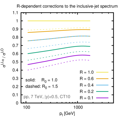
The phenomenological relevance of the small-$R$ terms is illustrated in Fig. 1, which shows the ratio of the jet spectrum with small-$R$ resummation effects to the LO jet spectrum. For this and a number of later plots, the $p_{t}$ and rapidity ranges and the collider energy choice correspond to those of ATLAS measurements Aad:2014vwa , to which we will later compare our results. We show the impact of resummation for a range of $R$ values from $0.1$ to $1.0$ and two $R_{0}$ choices. The smallest $R$ values typically in use experimentally are in the range $0.2$–$0.4$ and one sees that the fragmentation of partons into jets brings up to $40\%$ reduction in the cross section for the smaller of these radii. The fact that the small-$R$ effects are substantial is one of the motivations for our work here.

From the point of view of phenomenological applications, the question that perhaps matters more is the impact of corrections beyond NLO (or forthcoming NNLO), since fixed order results are what are most commonly used in comparisons to data. This will be most easily quantifiable when we discuss matched results in sections 3 and 4. Note that there was already some level of discussion of effects beyond fixed order in Ref. Dasgupta:2014yra , in terms of an expansion in powers of $t$. However comparisons to standard fixed order refer to an expansion in $\alpha_{s}$, which is what we will be using throughout this article. A brief discussion of the different features of $t$ and $\alpha_{s}$ expansions is given in Appendix A.

2.2 Range of validity of the small-$R$ approximation and effects beyond LL_R

In order to carry out a reliable phenomenological study of small-$R$ effects it is useful to ask two questions about the validity of our LL_R small-$R$ approach. Firstly we wish to know from what radii the underlying small-angle approximation starts to work. Secondly, we want to determine the potential size of small-$R$ terms beyond LL_R accuracy.

To investigate the first question we take the full next-to-leading-order (NLO) calculation for the inclusive jet spectrum from the NLOJet++ program nlojet , and look at the quantity $\Delta_{1}(p_{t},R,R_{\text{ref}})$, where

$$\Delta_{i}(p_{t},R,R_{\text{ref}})\equiv\frac{\sigma_{i}(p_{t},R)-\sigma_{i}(p_{t},R_{\text{ref}})}{\sigma_{0}(p_{t})}\,.$$ (3)

Here $\sigma_{i}(p_{t})$ corresponds to the order $\alpha_{s}^{2+i}$ contribution to the inclusive jet cross section in a given bin of $p_{t}$. This can be compared to a similar ratio, $\Delta_{1}^{\text{LL${}_{R}$}}(p_{t},R,R_{\text{ref}})$, obtained from the NLO expansion of Eq. (1) instead of the exact NLO result. The quantity $R_{\text{ref}}$ here is some small reference radius at which one expects the small-$R$ approximation to be valid; we choose $R_{\text{ref}}=0.1$. Fig. 2 (left) shows the comparison of $\Delta_{1}$ (filled squares) and $\Delta_{1}^{\text{LL${}_{R}$}}$ (crosses) as a function of $p_{t}$ for several different $R$ values. One sees very good agreement between $\Delta_{1}$ and $\Delta_{1}^{\text{LL${}_{R}$}}$ for the smaller $R$ values, while the agreement starts to break down for $R$ in the vicinity of $1$–$1.5$. This provides grounds for using the small-$R$ approximation for $R$ values $\lesssim 0.6$ and motivates a choice of $R_{0}$ in range $1$–$1.5$. We will take $R_{0}=1$ as our default, and use $R_{0}=1.5$ as a probe of resummation uncertainties.

Figure 2: Left: Comparison of the $R$ dependence in the exact and small-$R$ approximated NLO expansion, using Eq. (3), shown as a function of jet transverse momentum $p_{t}$, for $\sqrt{s}=7\,\mathrm{TeV}$ in the rapidity region $|y|<0.5$. Right: comparison of $\Delta_{1+2}(p_{t},R,R_{\text{ref}})$ and $\Delta_{1+2}^{\text{LL${}_{R}$}}(p_{t},R,R_{\text{ref}})$ (cf. Eq. (5)). In both plots CT10 NLO PDFs Lai:2010vv are used, while the renormalisation and factorisation scales are set equal to the $p_{t}$ of the highest-$p_{t}$ $R=1$ jet in the event (this same scale is used for all $R$ choices in the final jet finding).

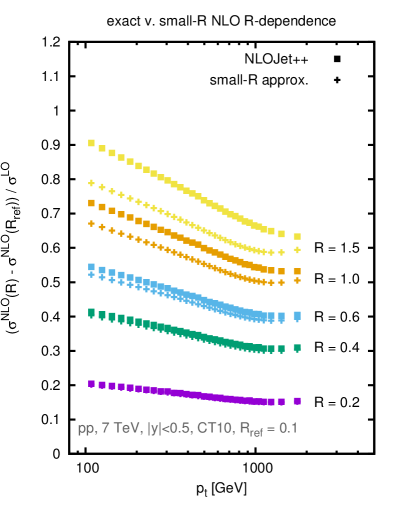
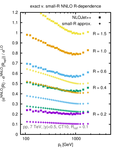
Next let us examine effects of subleading small-$R$ logarithms, terms that come with a factor $\alpha_{s}^{n}\ln^{n-1}R$ relative to the Born cross section. While there has been some work investigating such classes of terms in Refs. Becher:2015hka ; Chien:2015cka , those results do not apply to hadron-collider jet algorithms. Instead, here we examine the $R$ dependence in the NNLO part of the inclusive jet cross section to evaluate the size of these terms. Because the $R$ dependence starts only at order $\alpha_{s}^{3}$, we can use the NLO 3-jet component of the NLOJet++ program to determine these terms. More explicitly, we use the fact that

$$\sigma^{\text{NNLO}}(R)-\sigma^{\text{NNLO}}(R_{\text{ref}})=\sigma^{\text{NLO}_{3j}}(R)-\sigma^{\text{NLO}_{3j}}(R_{\text{ref}})\,.$$ (4)

To determine this difference in practice, for each event in the NLOJet++ 3-jet run we apply the following procedure: we cluster the event with radius $R$ and for each resulting jet add the event weight to the jet’s corresponding $p_{t}$ bin; we then recluster the particles with radius $R_{\text{ref}}$ and for each jet subtract the event weight from the corresponding $p_{t}$ bin. For this procedure to give a correct answer, it is crucial not to have any 3-jet phasespace cut in the NLO 3-jet calculation (i.e. there is no explicit requirement of a 3rd jet).

Hence, we can then examine

$$\Delta_{1+2}(p_{t},R,R_{\text{ref}})\equiv\Delta_{1}(p_{t},R,R_{\text{ref}})+\Delta_{2}(p_{t},R,R_{\text{ref}})$$ (5)

and its corresponding LL_R approximation, $\Delta_{1+2}^{\text{LL${}_{R}$}}(p_{t},R,R_{\text{ref}})$. The reason for including both NLO and NNLO terms is to facilitate comparison of the size of the results with that of the pure NLO piece. The results for $\Delta_{1+2}$ (filled squares) and $\Delta_{1+2}^{\text{LL${}_{R}$}}$ (crosses) are shown in Fig. 2 (right). The difference between the crosses in the left-hand and right-hand plots is indicative of the size of the NNLO LL_R contribution. At small $R$, the difference between the crosses and solid squares in the right-hand plot gives the size of the NLL_R contribution at NNLO. It is clear that this is a substantial contribution, of the same order of magnitude as the LL_R contribution itself, but with the opposite sign. Ideally one would therefore carry out a full NLL_R calculation. That, however, is beyond the scope of this article.

Instead we will include a subset of the subleading $\ln R$ terms by combining the LL_R resummation with the exact $R$ dependence up to NNLO fixed order, i.e. the terms explicitly included in the solid squares in Fig. 2.

3 Matching NLO and LL_R

For phenomenological predictions, it is necessary to combine the LL_R resummation with results from fixed-order calculations. In this section we will first examine how to combine LL_R and NLO results, and then proceed with a discussion of NNLO corrections.

3.1 Matching prescriptions

One potential approach for combining LL_R and NLO results would be to use an additive type matching,

$$\sigma^{\text{NLO}+\text{LL${}_{R}$},\text{add.}}(R)=\sigma^{\text{LL${}_{R}$}}(R)+\sigma_{1}(R)-\sigma^{\text{LL${}_{R}$}}_{1}(R)\,,$$ (6)

where $\sigma_{1}(R)$ denotes the pure NLO contribution to the inclusive jet spectrum (without the LO part, as in section 2.2) and $\sigma^{\text{LL${}_{R}$}}_{1}(R)$ refers to the pure NLO contribution within the LL_R resummation. For compactness, the $p_{t}$ argument in the cross sections has been left implicit.

A simple, physical condition that the matching must satisfy is that in the limit $R\to 0$, the ratio of the matched result to the LO result should tend to zero perturbatively,

$$\frac{\sigma^{\text{NLO}+\text{LL${}_{R}$}}}{\sigma_{0}}\,\to 0\qquad\text{for $R\to 0$}\,.$$ (7)

Eq. (6) does not satisfy this property: while $\sigma^{\text{LL${}_{R}$}}/\sigma_{0}$ does tend to zero, the quantity $(\sigma_{1}-\sigma^{\text{LL${}_{R}$}}_{1})/\sigma_{0}$ instead tends to a constant for small $R$. We will therefore not use additive matching.

Another class of matching procedure is multiplicative matching. One simple version of multiplicative matching is given by

$$\sigma^{\text{NLO}+\text{LL${}_{R}$},\text{mult.simple}}=\frac{\sigma^{\text{LL${}_{R}$}}(R)}{\sigma_{0}}\times\left(\sigma_{0}+\sigma_{1}(R)-\sigma^{\text{LL${}_{R}$}}_{1}(R)\right)\,.$$ (8)

Because $\sigma^{\text{LL${}_{R}$}}_{1}(R)$ contains the same logs as those in $\sigma_{1}(R)$, the right hand bracket tends to a constant for small $R$ and all the $R$ dependence comes from the $\sigma^{\text{LL${}_{R}$}}(R)$ factor. Since $\sigma^{\text{LL${}_{R}$}}(R)$ tends to zero for $R\to 0$, Eq. (8) satisfies the condition in Eq. (7). The matching formula that we actually use is

$$\sigma^{\text{NLO}+\text{LL${}_{R}$}}=\left(\sigma_{0}+\sigma_{1}(R_{0})\right)\times\left[\frac{\sigma^{\text{LL${}_{R}$}}(R)}{\sigma_{0}}\times\left(1+\frac{\sigma_{1}(R)-\sigma_{1}(R_{0})-\sigma^{\text{LL${}_{R}$}}_{1}(R)}{\sigma_{0}}\right)\right],$$ (9)

where $R_{0}$ is taken to be the same arbitrary radius of order $1$ that appears in $\sigma^{\text{LL${}_{R}$}}(R)$ as defined in Eq. (1). Compared to Eq. (8), we have explicitly separated out a factor $(\sigma_{0}+\sigma_{1}(R_{0}))$. As with Eq. (8), at small-$R$ the entire $R$ dependence comes from the $\sigma^{\text{LL${}_{R}$}}(R)$ factor, thus ensuring that Eq. (7) is satisfied. Eq. (9) has the advantage over Eq. (8) that matching will be simpler to extend to NNLO+LL_R, which is why we make it our default choice.

Eq. (9) has a simple physical interpretation: the left-hand factor is the cross section for producing a jet of radius $R_{0}$ and is effectively a stand-in for the normalisation of the (ill-defined) partonic scattering cross section, i.e. we equate partons with jets with radius $R_{0}\sim 1$. The right hand factor (in square brackets) then accounts for the effect of fragmentation on the cross section, including both the LL_R contribution and an exact NLO remainder for the difference between the cross sections at radii $R_{0}$ and $R$.

Even without a small-$R$ resummation, one can argue that the physical separation that is embodied in Eq. (9) is one that should be applied to normal NLO calculations. This gives us the following alternative expression for the NLO cross section

$$\sigma^{\text{NLO}\text{-mult.}}=\left(\sigma_{0}+\sigma_{1}(R_{0})\right)\times\left(1+\frac{\sigma_{1}(R)-\sigma_{1}(R_{0})}{\sigma_{0}}\right)\,,$$ (10)

i.e. the cross section for producing a small-radius jet should be thought of as the cross section for the initial partonic scattering, followed by the fragmentation of the parton to a jet. As in Eq. (9), we introduce a radius $R_{0}\sim 1$ to give meaning to the concept of a “parton” beyond leading order. It is straightforward to see that Eq. (10) differs from standard NLO only in terms of corrections at order $\alpha_{s}^{2}$ relative to LO.

3.2 Unphysical cancellations in scale dependence

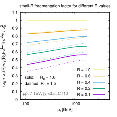
Let us now return to the resummed matched prediction, Eq. (9). The left and right-hand factors in that formula are shown separately in Fig. 3. The left-hand factor, corresponding to an overall normalisation for hard partonic scattering, is shown in the left-hand plot (divided by the LO to ease visualisation), while the small-$R$ fragmentation (i.e. right-hand) factor, which includes the resummation and matching contributions, is shown on the right. One sees that the two terms bring $K$-factors going in opposite directions. The overall normalisation has a $K$-factor that is larger than one and grows with $p_{t}$. Meanwhile the fragmentation effects generate a $K$-factor that is substantially below one for smaller $R$ values, with a relatively weak $p_{t}$ dependence.

The $p_{t}$ dependence of the two factors involves an interplay between two effects: on one hand, the fraction of gluons decreases at large $p_{t}$, as does $\alpha_{s}$; on the other hand the PDFs fall off more steeply at higher $p_{t}$, which enhances (positive) threshold logarithms in the normalisation factor and also increases the effect of small-$R$ logarithms in the fragmentation factor (i.e. reduces the fragmentation factor). We believe that the gentle increase of the fragmentation factor is due to the decrease in gluon fraction, partially counteracted by the increasing steepness of the PDFs. A similar cancellation is probably responsible for the flatness of the normalisation factor at low and moderate $p_{t}$’s, with threshold logarithms induced by the PDFs’ steepness driving the increase at the highest $p_{t}$’s.

We note also that both factors in Eq. (9) depend significantly on the choice of $R_{0}$, with two values being shown in Fig. 3, $R_{0}=1$ (solid) and $R_{0}=1.5$ (dashed). However in the full results, Eqs. (9) and (10), the $R_{0}$ dependence in cancels up to NLO, leaving a residual $R_{0}$ dependence that corresponds only to uncontrolled higher-order terms.

Figure 3: Left: size of the matching normalisation factor (left-hand factor of Eq. (9), normalised to LO), shown v. $p_{t}$ for various $R$ values and two $R_{0}$ choices. Right: size of the matched small-$R$ fragmentation factor (right-hand factor of Eq. (9); similar results are observed for the right-hand factor of Eq. (10)). The results are shown for the scale choice $\mu_{R}=\mu_{F}=p_{t,\max}$, where $p_{t,\max}$ is the transverse momentum of the hardest jet in the event.

The partial cancellation between higher-order effects that takes place between the small-$R$ effects and the residual matching correction is somewhat reminiscent of the situation for jet vetoes in Higgs-boson production. There it has been argued that such a cancellation can be dangerous when it comes to estimating scale uncertainties. As a result, different schemes have been proposed to obtain a more reliable and conservative estimate, notably the Stewart-Tackmann Stewart:2011cf and jet-veto-efficiency Banfi:2012yh methods. Here we will take an approach that is similar in spirit to those suggestions (though somewhat closer to the jet-veto-efficiency method) and argue that for a reliable estimate of uncertainties, scale-dependence should be evaluated independently for the left and right-hand factors in Eqs. (9) and (10) (and also in Eq. (8)), and the resulting relative uncertainties on those two factors should be added in quadrature. We will always verify that the $R_{0}$ dependence (for just the central scale choice) is within our scale uncertainty band.

3.3 NLO+LL_R matched results

Figure 4: Inclusive jet cross section for $p_{t}>100\,\mathrm{GeV}$, as a function of $R$, normalised to the ($R$-independent) leading-order result. Left: the standard NLO result, compared to the “NLO-mult.” result of Eq. (10) and the NLO+LL_R matched result of Eq. (9). The scale uncertainty here has been obtained within a prescription in which the scale is varied simultaneously in the left and right-hand factors of Eqs. (9) and (10) (“correlated scale choice”). Right: the same plot, but with the scale uncertainties determined separately the left and right-hand factors of Eqs. (9) and (10), and then added in quadrature (“uncorrelated scale choice”). The plot also shows the NLO+LL_R result for $R_{0}=1.5$ at our central scale choice.

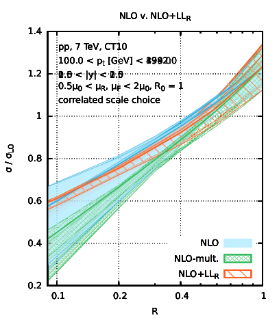
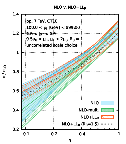
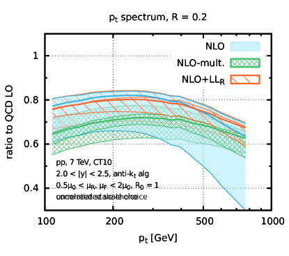
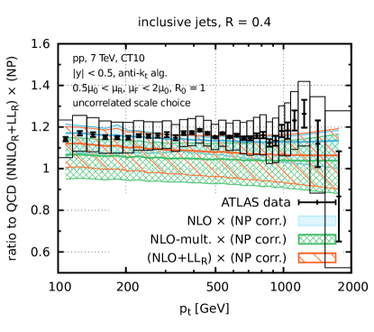
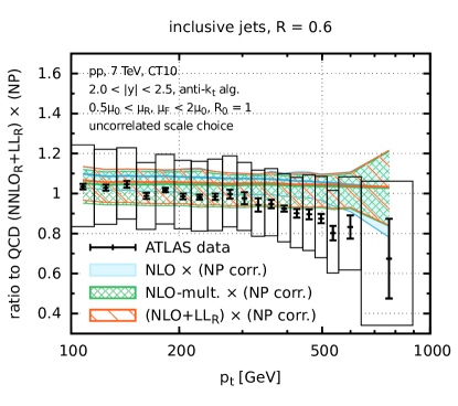
Fig. 4 shows the inclusive jet cross section integrated from $100\,\mathrm{GeV}$ to $1992\,\mathrm{GeV}$ (the full range covered by the ATLAS data Aad:2014vwa ), as a function of $R$, normalised to the leading order result. The left-hand plot shows the standard NLO result (light blue band), the “NLO-mult.” result of Eq. (10) (green band) and the NLO+LL_R matched result of Eq. (9) (orange band). To illustrate the issue of cancellation of scale dependence discussed in section 3.2, the scale uncertainty here has been obtained within a prescription in which the scale is varied in a correlated way in the left and right-hand factors of Eqs. (9) and (10). We adopt the standard convention of independent $\mu_{R}=\{\frac{1}{2},1,2\}\mu_{0}$ and $\mu_{F}=\{\frac{1}{2},1,2\}\mu_{0}$ variations around a central scale $\mu_{0}$, with the additional condition $\frac{1}{2}\leq\mu_{R}/\mu_{F}\leq 2$. Our choice for $\mu_{0}$ is discussed below.

One sees that in each of the 3 bands, there is an $R$ value for which the scale uncertainty comes close to vanishing, roughly $R=0.5$ for NLO, $R=0.3$ for “NLO-mult.” and $R=0.1{-}0.2$ for NLO+LL_R. We believe that this near-vanishing is unphysical, an artefact of a cancellation in the scale dependence between small-$R$ and overall normalisation factors, as discussed in the previous paragraph. One clear sign that the scale dependence is unreasonably small is that the NLO-mult. and NLO+LL_R bands differ by substantially more than their widths.

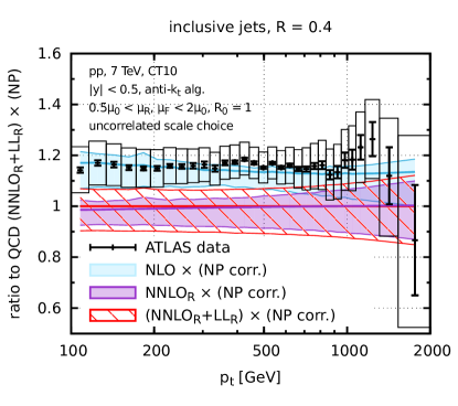
The right-hand plot of Fig. 4 instead shows uncertainty bands when one separately determines the scale variation uncertainty in the left-hand (normalisation) and the right-hand (small-$R$ matching) factors and then adds those two uncertainties in quadrature (“uncorrelated scale choice”; note that the NLO band is unchanged). Now the uncertainties remain fairly uniform over the whole range of $R$ and if anything increase towards small $R$, as one might expect. This uncorrelated scale variation is the prescription that we will adopt for the rest of this article.

Intriguingly, the NLO+LL_R result is rather close to the plain NLO prediction. Given the large difference between the NLO and NLO-mult. results, this is, we believe, largely a coincidence: if one examines yet smaller $R$, one finds that the NLO and NLO+LL_R results separate from each other, with the NLO and NLO-mult. results going negative for sufficiently small $R$, while the NLO+LL_R result maintains a physical behaviour.

Fig. 4 (right) also shows the impact of increasing $R_{0}$ to $1.5$. One sees a $5{-}10\%$ reduction in the cross section, however this reduction is within the uncertainty band that comes from the uncorrelated scale variation.

A comment is due concerning our choice of central scale, $\mu_{0}$. At NLO, for each event, we take $\mu_{0}$ to be the $p_{t}$ of the hardest jet in the event, $p_{t,\max}$. In NLO-like configurations, with at most 3 final-state partons, this hardest jet $p_{t}$ is independent of the jet radius and so we have a unique scale choice that applies to all jet radii. An alternative, widely used prescription is to use a separate scale for each jet, equal to that jet’s $p_{t}$. We disfavour this alternative because it leads to a spurious additional $R$ dependence, induced by inconsistent scale choices in real and virtual terms. Further details are given in Appendix B.

4 Matching to NNLO

4.1 Matching prescription

Given that full NNLO results for the inclusive cross section are likely to be available soon Currie:2013dwa , here we propose matching schemes for combining our small-$R$ resummed results with a full NNLO result. The direct analogue of Eq. (9) is

$$\sigma^{\text{NNLO}+\text{LL${}_{R}$}}=\left(\sigma_{0}+\sigma_{1}(R_{0})+\sigma_{2}(R_{0})\right)\times\\ \times\Bigg{[}\frac{\sigma^{\text{LL${}_{R}$}}(R)}{\sigma_{0}}\times\Bigg{(}1+\Delta_{1+2}(R,R_{0})-\frac{\sigma^{\text{LL${}_{R}$}}_{1}(R)+\sigma^{\text{LL${}_{R}$}}_{2}(R)}{\sigma_{0}}\hskip 142.26378pt\\ -\frac{\sigma_{1}^{\text{LL${}_{R}$}}(R)\left(\sigma_{1}(R)-\sigma^{\text{LL${}_{R}$}}_{1}(R)\right)}{\sigma_{0}^{2}}-\frac{\sigma_{1}(R_{0})}{\sigma_{0}}\bigg{(}\Delta_{1}(R,R_{0})-\frac{\sigma^{\text{LL${}_{R}$}}_{1}(R)}{\sigma_{0}}\bigg{)}\Bigg{)}\Bigg{]}\,,$$ (11)

where the functions $\Delta_{1}$ and $\Delta_{1+2}$ were defined in Eq. (3) and (5) and we recall that $\sigma^{\text{LL${}_{R}$}}$ and its expansion are functions both of $R$ and $R_{0}$. As with our NLO+LL_R formula, Eq. (9), we have written Eq. (11) in terms of two factors: an overall normalisation for producing $R_{0}$-jets, together with a matched fixed-order and resummed result for the correction coming from fragmentation of the $R_{0}$ jet into small-$R$ jets. One comment here is that in Eq. (9) the matching part (big round brackets inside the square brackets) gave a finite result for $R\to 0$. The situation is different at NNLO because the LL_R resummation does not capture the $\alpha_{s}^{2}\ln 1/R^{2}$ (NLL_R) term that is present at fixed order and so the matching term has a residual $\alpha_{s}^{2}\ln 1/R^{2}$ dependence. This means that for sufficiently small-$R$, Eq. (11) can become unphysical. We have not seen any evidence of this occurring in practice, but one should keep in mind that for future work one might aim to resolve this in-principle problem either by incorporating NLL_R resummationor by choosing a different form of matching, for example one where the ${\cal O}\left(\alpha_{s}^{2}\right)$ parts of the matching correction are exponentiated, ensuring a positive-definite result. Note that with NLL_R resummation one could also use a formula analogous to Eq. (8),

$$\sigma^{\text{NNLO}+\text{NLL${}_{R}$},\text{mult.simple}}=\\ =\Bigg{(}\sigma_{0}+\sigma_{1}+\sigma_{2}-\sigma^{\text{NLL${}_{R}$}}_{1}-\sigma^{\text{NLL${}_{R}$}}_{2}-\frac{\sigma^{\text{NLL${}_{R}$}}_{1}}{\sigma_{0}}\left(\sigma_{1}-\sigma^{\text{NLL${}_{R}$}}_{1}\right)\Bigg{)}\times\frac{\sigma^{\text{NLL${}_{R}$}}}{\sigma_{0}}\,,$$ (12)

where each of the terms is evaluated at radius $R$.

As well as a matched result, it can be instructive to study a modification of the plain NNLO result, “NNLO-mult.”, in analogy with Eq. (10). This remains a fixed order result, but it factorises the production of large-$R_{0}$ jets from the fragmentation to small-$R$ jets,

$$\sigma^{\text{NNLO}\text{-mult.}}=\left(\sigma_{0}+\sigma_{1}(R_{0})+\sigma_{2}(R_{0})\right)\times\left(1+\Delta_{1+2}(R,R_{0})-\frac{\sigma_{1}(R_{0})}{\sigma_{0}}\Delta_{1}(R,R_{0})\right)\,.$$ (13)

It differs from $\sigma^{\text{NNLO}}$ only by terms beyond NNLO.

As in section 3.1, in Eqs. (11)–(13) we advocate varying scales separately in the normalisation and fragmentation factors, and also studying the $R_{0}$ dependence of the final result.

4.2 A stand-in for NNLO: NNLO_R

We have seen in section 2.2 that NNLO terms of the form $\alpha_{s}^{2}\ln 1/R^{2}$ that are not accounted for in our LL_R calculation can be large. Insofar as they are known, they should however be included in phenomenological studies. This specific class of terms can be taken into account in the context of a stand-in for the full NNLO calculation which contains the exact NNLO $R$ dependence and that we refer to as NNLO_R. It is constructed as follows:

$$\sigma^{\text{NNLO${}_{R}$}}(R,R_{m})\equiv\sigma_{0}+\sigma_{1}(R)+[\sigma_{2}(R)-\sigma_{2}(R_{m})],$$ (14)

which depends on an arbitrary angular scale $R_{m}$. Though neither $\sigma_{2}(R)$ nor $\sigma_{2}(R_{m})$ can be fully determined currently, their difference can be obtained from the same NLO 3-jet calculation that was used to examine $\Delta_{1+2}(p_{t},R,R_{\text{ref}})$ in Fig. 2 (right).

Since the full NNLO result has the property

$$\sigma^{\text{NNLO}}(R)=\sigma^{\text{NNLO${}_{R}$}}(R,R_{m})+\sigma_{2}(R_{m})\,,$$ (15)

the use of $\sigma^{\text{NNLO${}_{R}$}}(R,R_{m})$ instead of $\sigma^{\text{NNLO}}(R)$ is equivalent to the assumption that $\sigma_{2}(R_{m})$ vanishes. In practice we will take $R_{m}=1$, independently of $p_{t}$.

One point to be aware of is that $\sigma^{\text{NNLO${}_{R}$}}(R,R_{m})$ and $\sigma^{\text{NNLO}}(R)$ have parametrically different scale dependence. On one hand, the $\sigma_{2}(R)$ term in $\sigma^{\text{NNLO}}(R)$ fully cancels the (relative) ${\cal O}\left(\alpha_{s}^{2}\right)$ scale variation that is left over from $\sigma_{0}$ and $\sigma_{1}$, leaving just ${\cal O}\left(\alpha_{s}^{3}\right)$ dependence. On the other, in $\sigma^{\text{NNLO${}_{R}$}}(R,R_{m})$ the use of the $\sigma_{2}(R)-\sigma_{2}(R_{m})$ means that some residual ${\cal O}\left(\alpha_{s}^{2}\right)$ dependence is left over. In particular, for $R=R_{m}$ the scale dependence is identical to that at NLO. Accordingly, when estimating higher-order uncertainties in studies that use NNLO_R results, we do not explicitly need to vary $R_{m}$, since the ${\cal O}\left(\alpha_{s}^{2}\right)$ uncertainty that it brings should already be accounted for in the scale variation.

Our central scale choice for any given event will be $\mu_{0}=p_{t,\max}^{R=1}$, the transverse momentum of the hardest jet in the event as clustered with $R=1$. This is analogous to the choice of $p_{t,\max}$ used at NLO, except that at NNLO one needs to explicitly specify $R$ since $p_{t,\max}$ can depend on the jet clustering. The logic for taking $p_{t,\max}$ at a fixed jet radius of $1$, independently of the $R$ used in the clustering for the final jet spectrum, is that one obtains a unique scale for the event as a whole and avoids mixing scale-variation effects with $R$ dependence. Another potential choice that we did not investigate is to take the averaged $p_{t}$ of the two hardest jets. As long as the jets are obtained with a clustering radius $\sim 1$ such a choice is expected to be good at minimising the impact both of initial-state and final-state radiation, whereas our $p_{t,\max}$ choice has some sensitivity to initial-state radiation.

4.3 Results at NNLO_R and NNLO_R+LL_R

Figure 5: Left: comparison of the NLO, NNLO_R and NNLO_R-mult. results for the inclusive jet cross section for $p_{t}>100\,\mathrm{GeV}$, as a function of $R$, normalised to the LO result. Right, corresponding comparison of NLO, NNLO_R and NNLO_R+LL_R together with the central curve for NNLO_R+LL_R when $R_{0}$ is increased to $1.5$. In both plots, for the NNLO_R-mult. and NNLO_R+LL_R results the scale-dependence has been evaluated separately in the normalisation and fragmentation contributions and added in quadrature to obtain the final uncertainty band.

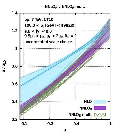
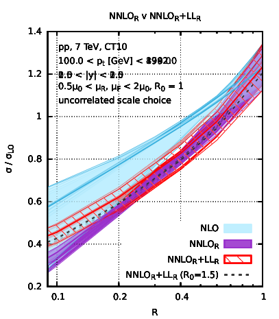
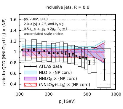
Let us start by examining the NNLO_R result, shown versus $R$ as the purple band in Fig. 5 (left), together with the NNLO_R-mult. results using Eq. (13) and the NLO band. One sees that the $R$ dependence of the NNLO_R result is steeper than in the NLO result, especially for $R\gtrsim 0.2$. This pattern is qualitatively in line with one’s expectations from Fig. 2 (right) and will hold also for the full NNLO calculation, which differs from NNLO_R only by an $R$-independent (but $p_{t}$ and scale-dependent) additive constant. The point of intersection between the NLO and NNLO_R results, at $R=1$, is instead purely a consequence of our choice of $R_{m}=1$ in Eq. (14). Thus at $R=1$, both the central value and scale dependence are by construction identical to those from the NLO calculation.

The left-hand plot of Fig. 5 also shows the NNLO_R-mult. result. Relative to what we saw when comparing NLO and NLO-mult., the most striking difference here is the much better agreement between NNLO_R and NNLO_R-mult., with the two generally coinciding to within a few percent. For $R\gtrsim 0.4$, this good agreement between different approaches carries through also to the comparison between NNLO_R and NNLO_R+LL_R. However, for yet smaller values of $R$, the NNLO_R+LL_R result starts to be substantially above the NNLO_R and NNLO_R-mult. ones. This is because the NNLO_R and NNLO_R-mult. results have unresummed logarithms that, for very small-$R$, cause the cross section to go negative, whereas the resummation ensures that the cross section remains positive (modulo the potential issue with unresummed NLL_R terms that remain after matching).

Comparing the NNLO_R+LL_R result to the NLO+LL_R of Fig. 4 (right), one finds that the central value of the NNLO_R+LL_R prediction starts to lie outside the NLO+LL_R uncertainty band for $R\lesssim 0.5$. This highlights the importance of the NNLO corrections, and in particular of terms with subleading $\ln 1/R^{2}$ enhancements. Finally, the dependence on the choice of $R_{0}$ is slightly reduced at NNLO_R+LL_R compared to NLO+LL_R and it remains within the scale-variation uncertainty band.

To help complete the picture, we also show results as a function of $R$ in a high-$p_{t}$ bin, $1530<p_{t}<1992\,\mathrm{GeV}$ in Fig. 6. Most of the qualitative observations that we discussed above remain true also for high $p_{t}$. The main difference relative to the $p_{t}>100\,\mathrm{GeV}$ results is that scale uncertainty bands generally grow larger. This is perhaps due to threshold effects and might call for the inclusion of threshold resummation, see e.g. Ref. deFlorian:2013qia and references therein. Figs. 7 and 8 show the jet spectrum as a function of $p_{t}$, normalised to the LO result, for $R=0.2$ and two rapidity bins. Again, the conclusions are similar.

Figure 6: Same as figure 4, but focusing only on the high $p_{t}$ bin. Both plots use an uncorrelated scale variation in the normalisation and fragmentation factors.

Figure 7: Left: the NLO inclusive jet spectrum as a function of $p_{t}$, normalised to LO, together with the “NLO-mult.” result and the NLO+LL_R matched results for $R=0.2$. The cross section is shown for the rapidity bin $|y|<0.5$. The bands give the scale uncertainty obtained using an uncorrelated scale choice. Right: analogous plots with the NNLO_R and NNLO_R+LL_R predictions.

Figure 8: Same as figure 7 but showing the cross section in the rapidity bin $2<|y|<2.5$.

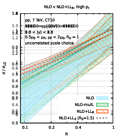
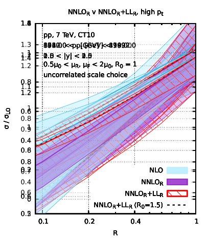
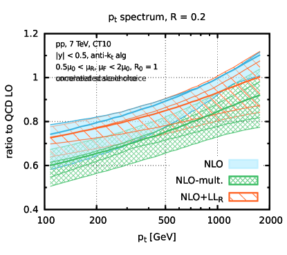
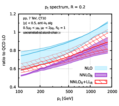
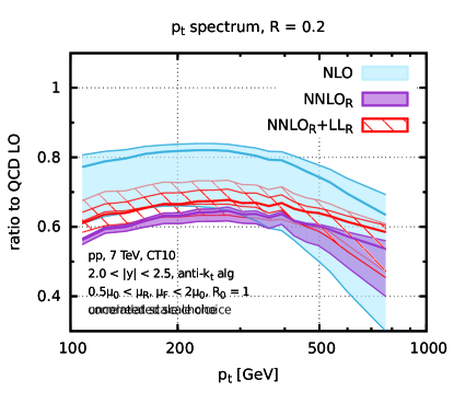
All of the predictions shown here have been obtained with the choice $R_{m}=1$ in Eq. (14), equivalent to the assumption that $\sigma_{2}(R_{m}=1)=0$ in Eq. (15). For a discussion of how the predictions change if $\sigma_{2}(R_{m}=1)$ is non-zero, the reader is referred to section 4.4.

To conclude this section, our main observation is that LL_R and NNLO terms both have a significant impact on the $R$ dependence of the inclusive jet spectrum, with the inclusion of both appearing to be necessary in order to obtain reliable predictions for $R\lesssim 0.4$. In particular, if NNLO and NLO coincide for $R=1$, then for $R=0.4$ the NNLO results will be about $20\%$ below the NLO ones. Going down to $R=0.2$, one sees that even with NNLO corrections resummation of small-$R$ logarithms is important, having a further $10\%$ effect.

4.4 Impact of finite two-loop corrections

In our NNLO_R-based predictions, we have all elements of the full NNLO correction except for those associated with 2-loop and squared 1-loop diagrams (and corresponding counterterms).

Here, we examine how our results depend on the size of those missing contributions. We introduce a factor $K$ that corresponds to the NNLO/NLO ratio for a jet radius of $R_{m}$:

$$\sigma^{\text{NNLO}_{R,K}}(R_{m})=K\times\sigma^{\text{NLO}}(R_{m})\,.$$ (16)

For other values of the jet radius, we have

$$\sigma^{\text{NNLO}_{R,K}}(R)=\sigma_{0}\left[1+\frac{\sigma_{1}(R)}{\sigma_{0}}+\Delta_{2}(R,R_{m})+(K-1)\times\left(1+\frac{\sigma_{1}(R_{m})}{\sigma_{0}}\right)\right]\,.$$ (17)

As before, we will take $R_{m}=1.0$. One could attempt to estimate $K$ from the partial NNLO calculation of Ref. Currie:2013dwa , however given that this calculation is not yet complete, we prefer instead to leave $K$ as a free parameter and simply examine the impact of varying it.

Figure 9: The same as figure 5, but applying a K-factor of 1.10 to the NNLO_R prediction, as an estimate of the potential impact of the full NNLO calculation.

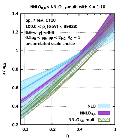
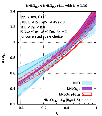
In Fig. 9, we show the impact of taking $K=1.10$, to be compared to Fig. 5, which corresponds to $K=1$. As $K$ is increased, one sees that NNLO_R,K and NNLO_R,K+LL_R start to agree over a wider range of $R$. This behaviour can be understood by observing there are two effects that cause NNLO_R,K and NNLO_R,K+LL_R to differ: on one hand the small-$R$ resummation prevents the cross section from going negative at very small radii, raising the prediction in that region relative to NNLO_R and reducing the overall $R$ dependence. On the other hand, the normalisation (first) factor in Eq. (11), which is larger than $1$, multiplies the full NNLO $R$ dependence that is present in the fragmentation (second) factor, thus leading to a steeper $R$ dependence than in pure NNLO_R,K. With $K=1$, the first effect appears to dominate. However as $K$ is increased, the second effect is enhanced and then the two effects cancel over a relatively broad range of $R$ values.

To put it another way, in the NNLO_R,K result the $K$ factor acts additively, shifting the cross section by the same amount independently of $R$. In the NNLO_R,K+LL_R result, the $K$ factor acts multiplicatively, multiplying the cross section by a constant factor independently of $R$. By construction, the two always agree for $R=R_{0}=1$. With $K=1$, NNLO_R,K is below NNLO_R,K+LL_R at small $R$, but the additive shift for $K>1$ brings about a larger increase of NNLO_R,K than the multiplicative factor for NNLO_R,K+LL_R, because $\sigma/\sigma(R_{0})$ is smaller than one.

Another point to note is that while in Fig. 5 the NNLO_R-mult. and NNLO_R results agreed over the full range of $R$, that is no longer the case with $K=1.1$: this is because NNLO_R-mult. acquires a multiplicative correction, as compared to the additive correction for NNLO_R,K. Therefore one strong conclusion from our study is that independently of the size of the NNLO $K$-factor, plain fixed order calculations at NNLO are likely to be insufficient for $R\lesssim 0.4$.

4.5 Comparison to POWHEG

One widely used tool to study the inclusive jet spectrum is POWHEG’s dijet implementation Alioli:2010xa . Insofar as parton showers should provide LL_R accuracy and POWHEG guarantees NLO accuracy, POWHEG together with a shower should provide NLO+LL_R accuracy. It is therefore interesting to compare our results to those from the POWHEG BOX V2’s dijet process (v3132), which are obtained here using a generation cut bornktmin of $50\,\mathrm{GeV}$ and a suppression factor bornsuppfact of $500\,\mathrm{GeV}$. We have used it with Pythia 8 (v8.186 with tune 4C Corke:2010yf ) for the parton shower, Pythia 6 (v6.428 the Perugia 2011 tune Skands:2010ak ) and with Herwig 6 (v6.521 with the AUET2-CTEQ6L1 tune ATLAS:2011gmi ). We examine the results at parton level, with multiple-parton interaction (MPI) effects turned off. Since the Pythia 6 and Pythia 8 results are very similar we will show only the latter. In the case of Pythia 8, we include an uncertainty band from the variation of scales in the generation of the POWHEG events.

Figure 10: Top: comparison between the NNLO_R-based results and POWHEG+Herwig 6 (left) and POWHEG+Pythia 8 (right), shown as a function of $R$, integrated over $p_{t}$ for $p_{t}>100\,\mathrm{GeV}$. Bottom right: comparison of POWHEG+Pythia 8 with NNLO_R-based results, where the latter have an additional NNLO $K$-factor of $1.15$.

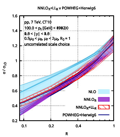
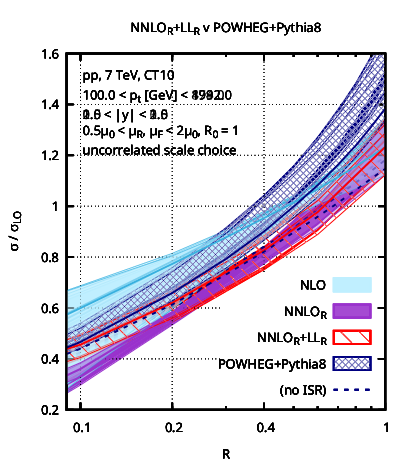
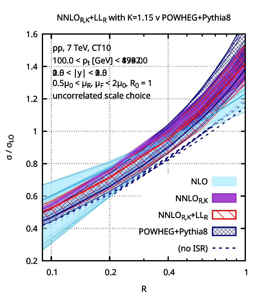
In Fig. 10, we show the $p_{t}$-integrated cross section as a function of $R$. The dark blue band (or line) shows the predictions obtained from POWHEG. In the top left-hand plot one sees a comparison with POWHEG+Herwig 6, which agrees with the NNLO_R+LL_R result to within the latter’s uncertainty band, albeit with a slightly steeper $R$ dependence at large $R$ values. In the top right-hand plot, one sees a comparison with POWHEG+Pythia 8. There is reasonable agreement for small radii, however the POWHEG+Pythia 8 prediction has much steeper $R$ dependence and is substantially above the NNLO_R+LL_R result for $R=1$. Differences between Herwig and Pythia results with POWHEG have been observed before Aad:2011fc , though those are at hadron level, including underlying-event effects, which can introduce further sources of difference between generators.

One difference between the NNLO_R+LL_R results and those from POWHEG with a shower-generator is an additional resummation of running scales and Sudakov effects for initial-state radiation (ISR). To illustrate the impact of ISR, the dark-blue dashed curve shows how the POWHEG+Pythia 8 prediction is modified if one switches off initial-state radiation (ISR) in the shower. Though not necessarily a legitimate thing to do (and the part of the ISR included in the POWHEG-generated emission has not been switched off), it is intriguing that this shows remarkably good agreement with the NNLO_R+LL_R results over the full $R$ range. This might motivate a more detailed future study of the interplay between ISR and the jet spectrum. Note that, as shown in Alioli:2010xa , nearly all the $R$ dependence of the POWHEG+parton-shower result comes from the parton shower component. It is not so straightforward to examine Herwig with ISR turned off so we have not included this in our study.

Given the differences between POWHEG +Pythia 8 and our NNLO_R+LL_R results, it is also of interest to examine what happens for $K\neq 1$. We can tune $K$ so as to produce reasonable agreement between NNLO_R,K+LL_R and POWHEG+Pythia 8 for $R=1$ and this yields $K\simeq 1.15$, which we have used in the bottom-right plot. Then it turns out that both predictions agree within uncertainty bands not just at $R=1$, but over the full $R$ range. In this context it will be particularly interesting to see what effective value of $K$ comes out in the full NNLO calculation. Note that the patterns of agreement observed between different predictions depend also on $p_{t}$ and rapidity. For a more complete picture we refer the reader to our online tool OnlineTool .

5 Hadronisation

Before considering comparisons to data, it is important to examine also the impact of non-perturbative effects. There are two main effects: hadronisation, namely the effect of the transition from parton-level to hadron-level; and the underlying event (UE), generally associated with multiple interactions between partons in the colliding protons. Hadronisation is enhanced for small radii so we discuss it in some detail.

One way of understanding the effect of hadronisation and the underlying event is to observe that they bring about a shift in $p_{t}$. This can to some extent be calculated analytically and applied to the spectrum Dasgupta:2007wa . An alternative, more widespread approach is to use a Monte Carlo parton shower program to evaluate the ratio of hadron to parton level jet spectra and multiply the perturbative prediction by that ratio. One of the advantages of the analytical hadronisation approaches is that they can matched with the perturbative calculation, e.g. as originally proposed in Ref. Dokshitzer:1995zt . In contrast, a drawback of the Monte Carlo hadronisation estimates is that the definition of parton-level in a MC simulation is quite different from the definition of parton level that enters a perturbative calculation: in particular showers always include a transverse momentum cutoff at parton level, while perturbative calculations integrate transverse momenta down to zero.

To help guide our choice of method, we shall first compare the $p_{t}$ shift as determined in Ref. Dasgupta:2007wa with what is found in modern Monte Carlo tunes. We first recall that the average shift should scale as $1/R$ (see also Refs. Korchemsky:1994is ; Seymour:1997kj ) for hadronisation and as $R^{2}$ for the underlying event (see also Ref. Cacciari:2008gn ). For small-$R$ jets, hadronisation should therefore become a large effect, while the underlying event should vanish. By relating the hadronisation in jets to event-shape measurements in DIS and $e^{+}e^{-}$ collisions in a dispersive-type model Dokshitzer:1995zt ; Dokshitzer:1995qm , Ref. Dasgupta:2007wa argued that the average $p_{t}$ shift should be roughly

$$\left\langle\smash{\Delta p_{t}}\right\rangle\simeq-\frac{C}{C_{F}}\left(\frac{1}{R}+{\cal O}\left(1\right)\right)\times 0.5\,\mathrm{GeV}\,,$$ (18)

where $C$ is the colour factor of the parton initiating the jet, $C_{F}=\frac{4}{3}$ for a quark and $C_{A}=3$ for a gluon. Those expectations were borne out by Monte Carlo simulations at the time, with a remarkably small ${\cal O}\left(1\right)$ term. Eq. (18) translates to a $-6\,\mathrm{GeV}$ shift for $R=0.2$ gluon-initiated jets. On a steeply falling spectrum, such a shift can modify the spectrum significantly.

Figure 11: The average shift in jet $p_{t}$ induced by hadronisation in a range of Monte Carlo tunes, for $R=0.4$ and $R=0.2$ jets, both quark and gluon induced. The shift is shown as a function of jet $p_{t}$ and is rescaled by a factor $RC_{F}/C$ ($C=C_{F}$ or $C_{A}$) in order to test the scaling expected from Eq. (18). The left-hand plot shows results from the AUET2 ATLAS:2011gmi tune of Herwig 6.521 Corcella:2000bw ; Corcella:2002jc and the Monash 13 tune Skands:2014pea of Pythia 8.186 Sjostrand:2007gs , while the right-hand plot shows results from the Z2 Field:2010bc and Perugia 2011 Skands:2010ak ; Cooper:2011gk tunes of Pythia 6.428 Sjostrand:2006za . The shifts have been obtained by clustering each Monte Carlo event at both parton and hadron level, matching the two hardest jets in the two levels and determining the difference in their $p_{t}$’s. The simple analytical estimate of $0.5\,\mathrm{GeV}\pm 20\%$ is shown as a yellow band.

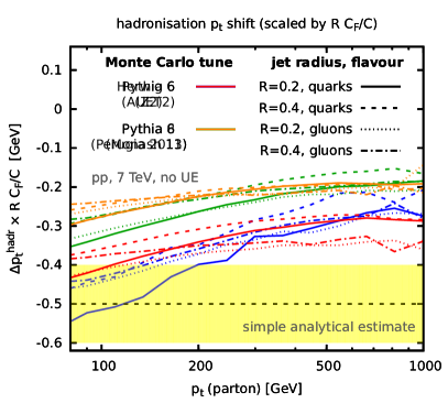
Fig. 11 shows the shift in $p_{t}$ in going from parton-level jets to hadron level jets, as a function of the jet $p_{t}$. Four modern Monte Carlo generator tunes are shown ATLAS:2011gmi ; Corcella:2000bw ; Corcella:2002jc ; Skands:2014pea ; Sjostrand:2007gs ; Skands:2010ak ; Cooper:2011gk ; Sjostrand:2006za , two in each plot. For each generator tune (corresponding to a given colour), there are four curves, corresponding to two values of $R$, $0.2$ and $0.4$ and both quark and gluon jets. The shifts have been rescaled by a factor $RC_{F}/C$. This means that if radius and colour-factor dependence in Eq. (18) are exact, then all lines of a given colour will be superposed. This is not exactly the case, however lines of any given colour do tend to be quite close, giving reasonable confirmation of the expected trend of $C/R$ scaling.

A further expectation of Eq. (18) is that the lines should cluster around $0.5\,\mathrm{GeV}$ and be $p_{t}$ independent. This, however, is not the case. Firstly, there is almost a factor of two difference between different generators and tunes, with Pythia 6 Perugia 2011 and Pythia 8 Monash 2013 both having somewhat smaller than expected hadronisation corrections. Secondly there is a strong dependence of the shift on the initial jet $p_{t}$, with a variation of roughly a factor of two between $p_{t}=100\,\mathrm{GeV}$ and $p_{t}=1\,\mathrm{TeV}$. Such a $p_{t}$ dependence is not predicted within simple approaches to hadronisation such as Refs. Korchemsky:1994is ; Dokshitzer:1995zt ; Dokshitzer:1995qm ; Dasgupta:2007wa . It was not observed in Ref. Dasgupta:2007wa because the Monte Carlo study there restricted its attention to a limited range of jet $p_{t}$, $55-70\,\mathrm{GeV}$. The event shape studies that provided support for the analytical hadronisation were also limited in the range of scales they probed, specifically, centre-of-mass energies in the range $40-200\,\mathrm{GeV}$ (and comparable photon virtualities in DIS). Note, however, that scale dependence of the hadronisation has been observed at least once before, in a Monte Carlo study shown in Fig. 8 of Ref. Salam:2001bd : effects found there to be associated with hadron masses generated precisely the trend seen here in Fig. 11. The $p_{t}$ dependence of those effects can be understood analytically, however we leave their detailed study in a hadron-collider context to future work. Experimental insight into the $p_{t}$ dependence of hadronisation might be possible by examining jet-shape measurements Aad:2011kq ; Chatrchyan:2012mec over a range of $p_{t}$, however such a study is also beyond the scope of this work.

In addition to the issues of $p_{t}$ dependence, one further concern regarding the analytical approach is that it has limited predictive power for the fluctuations of the hadronisation corrections from jet to jet. Given that the jet spectrum falls steeply, these fluctuations can have a significant impact on the final normalisation of the jet spectrum. One might address this with an extension of our analytical approach to include shape functions, e.g. as discussed in Ref. Korchemsky:1999kt .

In light of the above discussion, for evaluating hadronisation effects here, we will resort to the standard approach of rescaling spectra by the ratio of hadron to parton levels derived from Monte Carlo simulations.

Figure 12: Hadronisation (left) and underlying event (right) multiplicative corrections to the jet spectrum, as a function of $R$ for pp collisions at $7\,\mathrm{TeV}$. The top row shows results for $p_{t}>100\,\mathrm{GeV}$ and $|y|<0.5$, while the bottom row is for $p_{t}>1\,\mathrm{TeV}$. Six combinations of generator and tune are shown, and the yellow band corresponds to the envelope of the tunes.

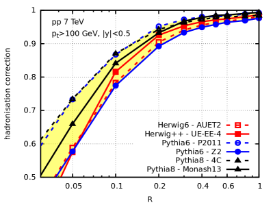
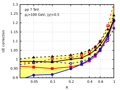
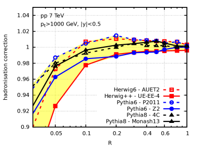
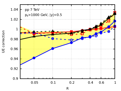
Fig. 12 shows, as a function of $R$, the ratio of hadron-level without UE to parton-level (left) and the ratio of hadron level with UE to hadron level without UE (right), for a range of Monte Carlo tunes. The results are shown for $p_{t}>100\,\mathrm{GeV}$ in the upper row and $p_{t}>1\,\mathrm{TeV}$ in the lower row. A wide range of $R$ values is shown, extending well below experimentally accessible values. Beyond the tunes shown in Fig. 11, here we also include the UE-EE-4 tune Gieseke:2012ft of Herwig++ 2.71 Bahr:2008pv ; Bellm:2013hwb and tune 4C Corke:2010yf of Pythia 8.186 Sjostrand:2007gs . To investigate the issue of possible mismatch between our analytic parton-level calculations and parton-level as defined in Monte Carlo simulations, we have considered a modification of Monte Carlo parton level where the transverse moment cutoff was taken to zero (an effective cutoff still remains, because of the use finite parton masses and $\Lambda_{\text{QCD}}$ in the shower, however this method can arguably still give a rough estimate of the size of the effect one is dealing with). One finds that taking the cutoff to zero changes the parton-level spectrum by a few percent effect. As this is somewhat smaller than the differences that we will shortly observe between tunes, it seems that for the time being it may not be too unreasonable to neglect it.

While there is a substantial spread in results between the different tunes in Fig. 12, the observed behaviours are mostly as expected, with hadronisation reducing the jet spectrum, especially at the smallest $R$ values, while the UE increases it, especially at large $R$ values. The magnitude of these effects is strongly $p_{t}$ dependent, with (roughly) a factor of ten reduction at not-too-small $R$ values when going from $p_{t}>100\,\mathrm{GeV}$ to $p_{t}>1\,\mathrm{TeV}$. Such a scaling is consistent with a rough $1/(Rp_{t})$ behaviour for hadronisation and $R^{2}/p_{t}$ behaviour for the UE (ignoring the slow changes in quark/gluon fraction and steepness of the spectrum as $p_{t}$ increases).

One surprising feature concerns the behaviour of the UE corrections at very small radii: firstly, in a number of the tunes the corrections tend to be smaller than $1$, suggesting that the multi-parton interactions (MPI) that are responsible for the UE remove energy from the core of the jet. For $R$ values in the range $0.4{-}1$, the effect of MPI is instead to add energy to the jet, as expected. Secondly, this loss of energy from the jet is not particularly suppressed at high $p_{t}$. The most striking example is the Z2 tune where there can be corrections of up to $7\%$ at $R=0.03$ (and even more at yet smaller $R$ values). The effect is somewhat reduced in the Z2-LEP tune, which has modified fragmentation parameters. One wonders if the mechanism for MPI generation might be inducing some form of factorisation breaking. A simple context in which to study this might be the high-$p_{t}$ inclusive hadron spectrum, where factorisation would imply that MPI should have no effect. While $k_{t}$-factorisation is believed to be broken for the inclusive hadron spectrum Collins:2007nk , we are not aware of definite statements concerning breaking of collinear factorisation.

6 Comparisons to data

Having formulated and studied the perturbative and non-perturbative contributions to the inclusive jet spectrum, we now consider comparisons with data. The purpose of this section is to highlight the relative sizes of different physical effects as compared to the precision of the data.

We will compare our predictions to the two datasets that have the smallest $R$ values: that from ALICE at centre-of-mass energy $\sqrt{s}=2.76\,\mathrm{TeV}$ with $R=0.2$ and $0.4$ Abelev:2013fn and that from ATLAS at $\sqrt{s}=7\,\mathrm{TeV}$ with $R=0.4$ and $0.6$ Aad:2014vwa .

All our results are obtained with CT10 NLO PDFs. This is the case also for our LO and NNLO_R results. For the latter, since NNLO_R does not correspond to full NNLO, it is justifiable to use NLO PDFs. One should also be aware that most modern PDF sets include inclusive jet-data in their fit. Accordingly they may have a bias associated with the theory choice that was used in their determination. With an updated theoretical framework, such as that used here, the PDFs would conceivably change and a complete study would benefit from refitting the PDFs. That is beyond the scope of this work and anyway more appropriately done once full NNLO results become available. For completeness, we have nevertheless briefly examined the impact of changing PDFs in the context of a pure LL_R calculation, examining also CT10nnlo Gao:2013xoa , CT14nlo, CT14nnlo Dulat:2015mca , MSTW2008nlo Martin:2009iq , MMHT2014nlo, MMHT2014nnlo Harland-Lang:2014zoa , NNPDF30_nlo_as_0118 and and NNPDF30_nnlo_as_0118 Ball:2014uwa . For $p_{t}$’s below $500\,\mathrm{GeV}$, most of these PDFs give results slightly above those from CT10, but by no more than $6\%$, which is modest relative to other uncertainties and differences that we will see below.

All fixed-order results are obtained with version 4.1.3 of the NLOJet++ program nlojet . Our central renormalisation and factorisation scale choice is $\mu_{0}=p_{t,\max}^{R=1}$, the transverse momentum of the hardest jet in the event as clustered with $R=1$. The envelope of independent variations of $\mu_{R}$ and $\mu_{F}$ by a factor of two (while maintaining $\frac{1}{2}\leq\mu_{R}/\mu_{F}\leq 2$) provides the perturbative uncertainty estimate. In the case of NLO-mult. and (N)NLO_(R)+LL_R results, the scale variation is performed independently for the normalisation and fragmentation factors and the uncertainty from the two factors is then added in quadrature. As explained in section 3, this is intended to avoid spuriously small scale uncertainties associated with cancellations between different physical contributions.

Non-perturbative corrections are taken as the average of the parton-to-hadron Monte Carlo correction factors (including hadronisation and UE) as obtained with the six different tunes discussed in section 5. The envelope of that set of six corrections provides our estimate of the uncertainty on the non-perturbative corrections, which is added in quadrature to the perturbative uncertainty.

In the case of the ATLAS data we will explore transverse momenta well above the electroweak (EW) scale, where EW corrections become substantial. The ATLAS collaboration accounted for these using the calculation of tree-level (${\cal O}\left(\alpha_{s}\alpha_{\text{EW}}\right)$) and loop (${\cal O}\left(\alpha_{s}^{2}\alpha_{\text{EW}}\right)$) EW effects from Ref. Dittmaier:2012kx . Here, since we concentrate on QCD effects, when showing the data we divide it by the EW corrections quoted by ATLAS.

6.1 Comparison to ALICE data

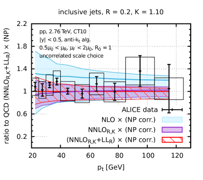
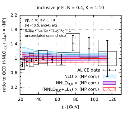
As a first application of small-$R$ resummation in comparisons to data, we look at the inclusive jet cross section in proton-proton collisions at $\sqrt{s}=2.76\,\mathrm{GeV}$ reported by the ALICE collaboration Abelev:2013fn . The measurements are in the $|y|<0.5$ rapidity range, with jets obtained using the anti-$k_{t}$ algorithm with a boost-invariant $p_{t}$ recombination scheme, for radii $R=0.2$ and $0.4$.

Figure 13: Non-perturbative corrections to the inclusive jet spectrum for the $p_{t}$ range, rapidity and centre-of-mass energy corresponding to the ALICE data Abelev:2013fn for $R=0.2$ (left) and $R=0.4$ (right). The results are shown separately for hadronisation, UE and the product of the two, and in each case include the average and envelope of the corrections from the six tunes discussed in section 5.

Figure 14: Comparison between a range of theoretical predictions for the inclusive jet spectrum and data from ALICE  at $\sqrt{s}=2.76\,\mathrm{TeV}$ Abelev:2013fn . The upper row is for $R=0.2$ and the lower one for $R=0.4$. The left-hand column shows NLO-based comparisons, while the right-hand one shows NNLO_R-based comparisons. Rectangular boxes indicate the size of systematic uncertainties on the data points, while the errors bars correspond to the statistical uncertainties. Results are normalised to the central NNLO_R+LL_R prediction (including non-perturbative corrections).

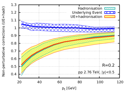
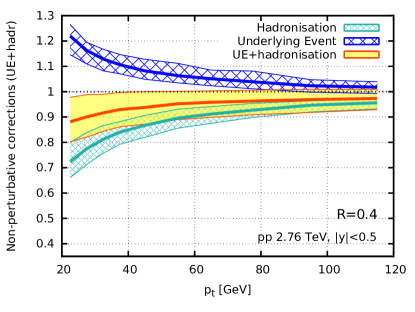
The non-perturbative corrections for hadronisation and underlying event are shown in Fig. 13. For $R=0.2$, non-perturbative corrections are largely dominated by hadronisation, with underlying event being a small effect, as expected for sufficiently small $R$. The net non-perturbative correction is about $-50\%$ at the lowest $p_{t}$ of $20\,\mathrm{GeV}$, while it decreases to about $-10\%$ at $100\,\mathrm{GeV}$. For $R=0.4$ there is a partial cancellation between hadronisation and UE, with a net impact of about $-10\%$ percent at low $p_{t}$ and a $5{-}10\%$ uncertainty.

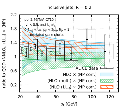
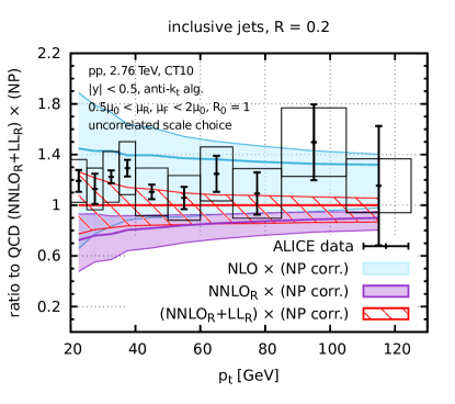
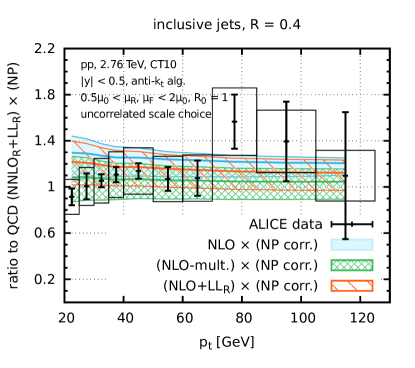
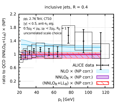
The comparison of our full results to the ALICE data is given in Fig. 14, as a ratio to the NNLO_R+LL_R theory prediction (including non-perturbative corrections). The top row shows the jet spectrum for $R=0.2$, while the lower row corresponds to $R=0.4$. The left-hand plots show NLO-based theory results. They all appear to be consistent with the data within their large uncertainties. The right-hand plots show NNLO_R-based theory (with plain NLO retained to facilitate cross-comparisons). In general the NNLO_R+LL_R results appear to provide the best match for the data, though they are slightly low. In particular, for $R=0.2$ where the differences between NNLO_R+LL_R and NNLO_R are substantial, almost $30\%$ at low $p_{t}$, there seems to be a preference for NNLO_R+LL_R. In contrast, at $R=0.4$ there is little difference between the two predictions though both are significantly more compatible with the data than is the plain NLO. In considering these statements, it is however important to keep several caveats in mind: the systematic uncertainties on the data and on the non-perturbative corrections (especially for $R=0.2$) are not negligible and a one-$\sigma$ shift could somewhat affect the conclusions. Furthermore, the currently unknown finite NNLO contribution (the difference between NNLO_R and full NNLO) may also have a relevant impact.

To further evaluate the compatibility of our results and the data we examine the ratio of the inclusive jet spectra at the two $R$ values, ${\cal R}(p_{t};R_{1},R_{2})=\sigma(p_{t};R_{1})/\sigma(p_{t};R_{2})$ with $R_{1}=0.2$ and $R_{2}=0.4$. This ratio is of interest because it allows us to directly study the $R$ dependence of the results and also because certain components of the uncertainties cancel in the ratio, in both the data and the theoretical prediction. In the experimental results, for example, the luminosity uncertainty cancels, as should part of the jet energy scale and resolution uncertainties. In the theoretical prediction, PDF uncertainties cancel. The ALICE collaboration’s results Abelev:2013fn explicitly include a determination of the ratio.

Earlier studies that focused on the $R$ ratios Soyez:2011np directly used the perturbative expansion for the cross-section ratio, rather than the ratio of perturbative predictions for the cross sections. That approach could be extended also to matched ratios, and one example of a NNLO+LL_R matching formula for the ratio would be

$${\cal R}^{\text{NNLO}+\text{LL${}_{R}$},\text{expand}}=\frac{\sigma^{\text{LL${}_{R}$}}(R_{1})}{\sigma^{\text{LL${}_{R}$}}(R_{2})}\times\Bigg{(}1+\Delta_{1+2}(R_{1},R_{2})-\Delta_{1+2}(R_{1},R_{2})\frac{\sigma_{1}(R_{2})}{\sigma_{0}}\\ \hskip 68.2866pt-\frac{\sigma_{1}^{\text{LL${}_{R}$}}(R_{1})+\sigma_{2}^{\text{LL${}_{R}$}}(R_{1})-\sigma_{1}^{\text{LL${}_{R}$}}(R_{2})-\sigma_{2}^{\text{LL${}_{R}$}}(R_{2})}{\sigma_{0}}\\ +\left(\frac{\sigma_{1}^{\text{LL${}_{R}$}}(R_{1})}{\sigma_{0}}-\Delta_{1}(R_{1},R_{2})\right)\frac{\sigma_{1}^{\text{LL${}_{R}$}}(R_{1})-\sigma_{1}^{\text{LL${}_{R}$}}(R_{2})}{\sigma_{0}}\Bigg{)}\,.$$ (19)

However, we prefer here to simply take the ratios of the relevant theory prediction (NLO, NNLO_R, NNLO_R+LL_R, etc.) at the two $R$ values, e.g.

$${\cal R}^{\text{NNLO+LL${}_{R}$}}=\frac{\sigma^{\text{NNLO${}_{R}$+LL${}_{R}$}}(R_{1})}{\sigma^{\text{NNLO${}_{R}$+LL${}_{R}$}}(R_{2})}\,.$$ (20)

This simple ratio has the same formal accuracy as (19) and fits better our primary goal, which is to predict inclusive jet cross sections and only examine their ratios for different $R$ values as a supplementary test. In the case of the results matched to LL_R resummation and of the (N)NLO-mult. results, the normalisation factor (with the cross section at radius $R_{0}$) cancels in the ratio, leaving only the fragmentation factor. For the NNLO_R-mult. and NNLO_R+LL_R results in particular, this means that any dependence on the unknown full NNLO $K$-factor (or, equivalently, the choice of $R_{m}$ in Eq. (14)) is eliminated, and the prediction for the ratio is identical to that which would be obtained with the full NNLO result. Accordingly, we will drop the subscript _R label in these cases, i.e. writing ${\cal R}^{\text{NNLO+LL${}_{R}$}}$ in Eq. (20) rather than ${\cal R}^{\text{NNLO${}_{R}$+LL${}_{R}$}}$.

To estimate the perturbative theoretical uncertainties on the ratio, we take the envelope of the ratios as determined for our seven renormalisation and factorisation scale choices. In the case of (N)NLO-mult. and (N)NLO+LL_R results, since the normalisation factor cancels, we only consider the component of the perturbative uncertainties associated with the fragmentation factor. We have verified that the effect of $R_{0}$ variation is contained within the scale-variation envelope. For the non-perturbative uncertainties, we take the envelope of the ratios of the corrections factors from different Monte Carlo tunes. The perturbative and non-perturbative uncertainties on the ratio are added in quadrature.

Figure 15: Comparison between a range of theoretical predictions for the inclusive jet cross-section ratio and data from ALICE  at $\sqrt{s}=2.76\,\mathrm{TeV}$ Abelev:2013fn . The left-hand column shows NLO-based comparisons, while the right-hand one shows NNLO_R-based comparisons. Rectangular boxes indicate the size of systematic uncertainties on the data points, while the errors bars correspond to the statistical uncertainties.

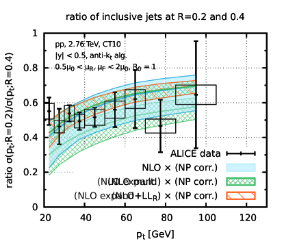
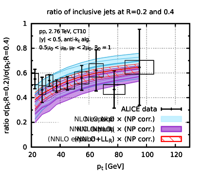
The comparison of the theory predictions with the measurements of the ALICE collaboration is presented in Fig. 15, at NLO accuracy on the left and at NNLO_(R)-based accuracy on the right. At first sight, it appears that the data have a considerably flatter $p_{t}$ dependence than any of the theory predictions. The latter all grow noticeably with increasing $p_{t}$, a consequence mainly of the $p_{t}$ dependence of the non-perturbative correction factor, cf. Fig. 13. Nevertheless, on closer inspection one sees that if one ignores the left-most data point then the remaining data points are compatible with the predicted $p_{t}$ dependence. The overall agreement is then best with the NNLO LL_R-based prediction. However, the sizes of the experimental uncertainties are such that it is difficult to draw firm conclusions.

We have also examined the impact of using Eq. (19) instead of (20) and find that the difference is small, no more than $5\%$. We have also examined the pure NNLO expansion of the ratio of cross sections, as used in Ref. Soyez:2011np and find that this too is quite similar to Eq. (20), much more so than the direct ratio of NNLO results, $\sigma^{\text{NNLO${}_{R}$}}(R_{1})/\sigma^{\text{NNLO${}_{R}$}}(R_{2})$. Thus our finding that we obtain reasonable agreement between Eq. (20) and the data is consistent with the observations of Ref. Soyez:2011np , which were based on expanded NNLO ratios.

6.2 Comparison to ATLAS data

Let us now turn to a comparison with the inclusive jet cross-sections reported by the ATLAS collaboration Aad:2014vwa , obtained from $4.5\text{ fb}^{-1}$ of proton-proton collisions at $\sqrt{s}=7\,\mathrm{TeV}$. Jets are identified with the anti-$k_{t}$ algorithm, this time with a usual $E$-scheme, taking radii $R=0.4$ and $0.6$. The measurements are doubly-differential, given as a function of jet $p_{t}$ and rapidity, and performed for $p_{t}>100\,\mathrm{GeV}$ and $|y|<3$. Note that given the difference in centre-of-mass energy, the lower $p_{t}$ for the ATLAS data, $100\,\mathrm{GeV}$, involves the same partonic $x$ range as $p_{t}=40\,\mathrm{GeV}$ for the ALICE data.

Figure 16: Non-perturbative corrections to the inclusive jet spectrum for the $p_{t}$ range, rapidity and centre-of-mass energy corresponding to the ATLAS data Aad:2014vwa for $R=0.4$ (left) and $R=0.6$ (right).

Figure 17: Comparison between a range of theoretical predictions for the inclusive jet spectrum and data from ATLAS at $\sqrt{s}=7\,\mathrm{TeV}$ Aad:2014vwa in the rapidity bin $|y|<0.5$. The upper row is for $R=0.4$ and the lower one for $R=0.6$. The left-hand column shows NLO-based comparisons, while the right-hand one shows NNLO_R-based comparisons. Rectangular boxes indicate the size of systematic uncertainties on the data points, while the errors bars correspond to the statistical uncertainties. Results are normalised to the central NNLO_R+LL_R prediction (including non-perturbative corrections).

Figure 18: Analogue of Fig. 17, but for the rapidity bin $2<|y|<2.5$.

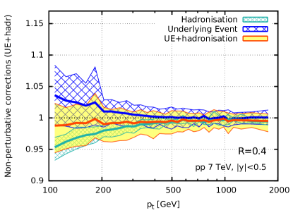
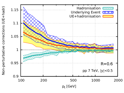
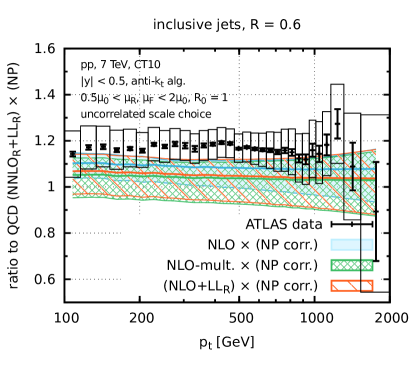
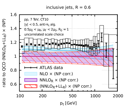
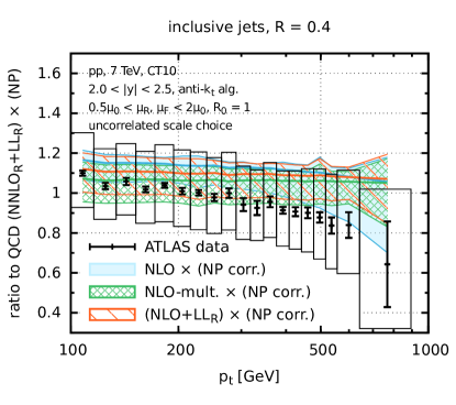
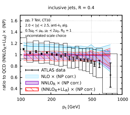
The hadronisation and underlying event corrections applied are shown in Fig. 16. As in the case of the ALICE data, for $R=0.4$ these two classes of correction mostly cancel. When increasing the jet radius to $R=0.6$, the hadronisation corrections shrink, while the UE corrections increase and now dominate, leaving a net effect of up to $6{-}7\%$ at the lowest $p_{t}$’s.

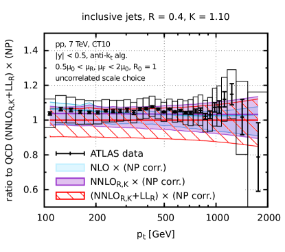
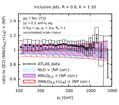
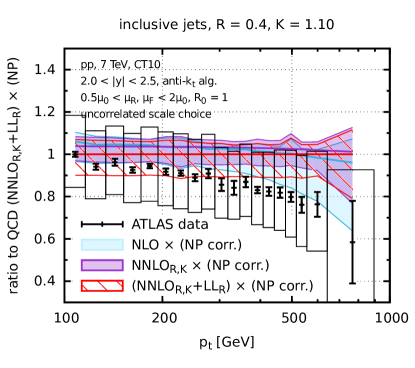
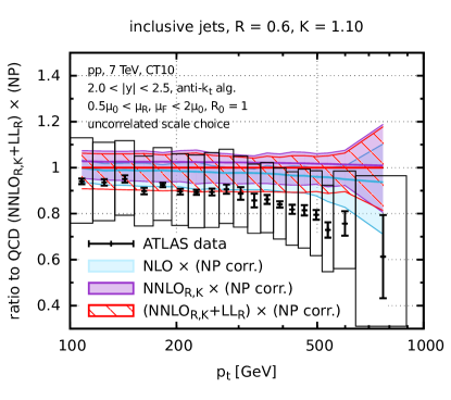
Figs. 17 and 18 show comparisons between data and theory for two rapidity bins, $|y|<0.5$ and $2.0<|y|<2.5$. At central rapidities the situation here contrasts somewhat with that for the ALICE data and in particular the inclusion of NNLO_R corrections worsens the agreement with data: over most of the $p_{t}$ range, the data points are about $15{-}20\%$ higher than than either NNLO_R or NNLO_R+LL_R (which are close to each other, as expected for $R\gtrsim 0.4$). Nevertheless, one encouraging feature of the NNLO_R-based predictions is that there is now a consistent picture when comparing $R=0.4$ and $R=0.6$, insofar as the ratio of data to NNLO_R-theory is essentially independent of $R$. This is not the case when comparing data and NLO predictions (cf. Fig. 5, which shows the steeper $R$ dependence of NNLO_R-based results as compared to NLO). We return to the question of $R$ dependence in more detail below.

In the forward rapidity bin, over most of the $p_{t}$ range, the data instead favours the NNLO_R-based predictions over NLO, while at high $p_{t}$ the data falls below all of the predictions. However the systematic uncertainties on the data are slightly larger than the difference with any of the theory predictions, making it difficult to draw any solid conclusions.

A significant positive 2-loop correction (cf. the discussion in sections 4.4, 4.5 and 6.3) would bring overall better agreement at central rapidities, but would worsen the agreement at forward rapidities. However, the finite 2-loop effects can be $p_{t}$ and rapidity dependent, making it difficult to draw any conclusions at this stage. Furthermore, one should keep in mind that adjustments in PDFs could affect different kinematic regions differently.

We close this section with an explicit comparison of the ratio of the jet spectra for the two different $R$ values. For the theoretical prediction, we proceed as discussed in the previous subsection, when we made a comparison with the ALICE data for such a ratio. We will not include EW effects, since in the ratio they appear to be at a level well below $1\%$.

Concerning the experimental results, the central value of the ratio can be obtained directly from the ATLAS data at the two $R$ values. However the ATLAS collaboration has not provided information on the uncertainties in the ratio. It has provided information ATLASHepData to facilitate the determination of correlations between $p_{t}$ and rapidity bins, specifically $10000$ Monte Carlo replicas of their data to aid in estimating statistical correlations, as well as a breakdown of systematic uncertainties into ${\cal O}\left(70\right)$ sources that are individually $100\%$ correlated across bins and totally uncorrelated with each other. The information is presented in a format such that, technically, it can also be used to estimate the uncertainties in the ratio of cross section for two $R$ values. However, we have been advised by the ATLAS collaboration that the degree of correlation between systematic uncertainties at different $R$ values is not well known. Accordingly, we label the uncertainties obtained in this way as “approx. uncert.” to emphasise that we do not have full knowledge of the experimental uncertainties in the ratio and that they are potentially larger than our estimate.

Figure 19: Comparison between a range of theoretical predictions for the inclusive jet cross-section ratio and data from ATLAS  at $\sqrt{s}=7\,\mathrm{TeV}$ Aad:2014vwa . The left-hand column shows NLO-based comparisons, while the right-hand one shows NNLO_(R)-based comparisons. Rectangular boxes indicate our estimated systematic uncertainties on the data points, while the errors bars correspond to the statistical uncertainties. Note that these estimates are known to be incomplete, insofar as the information provided by the ATLAS collaboration on its results is not intended to be used for the determination of uncertainties on cross section ratios at different radii.

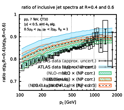
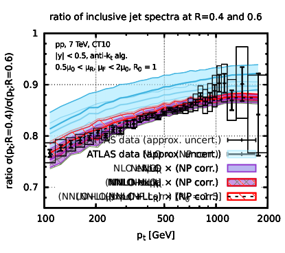
Keeping in mind this caveat, we show in Fig. 19 a comparison between various theoretical predictions for the cross section ratio at $R=0.4$ relative to $R=0.6$, together with the experimental data. One sees overall very good agreement with both the NNLO_R and NNLO+LL_R-based results, and substantially worse accord with NLO-based predictions (albeit consistent with pure NLO and NLO-mult. within their larger uncertainties).

6.3 Brief comparisons with an NNLO $K$-factor

For completeness, here we show the comparisons between theoretical predictions and data change when we introduce a two-loop $K$-factor for $R=R_{m}$, as described in section 4.4. Figures 20, 21 and 22 are to be compared to their counterparts in sections 6.1 and 6.2 i.e. Figs. 14, 17 and 18. In most cases, the changes that one observes are largely as expected, with a corresponding trivial rescaling of the observed data–theory ratio. One exception is in the case of the $R=0.2$ comparison to ALICE data, Fig. 20 (left), where with $K=1.10$ one observes that the NNLO_R,K results are now in very close accord with the NNLO_R,K+LL_R results. This is to be contrasted with the situation in Fig. 14. The difference is due to the fact that the $K$ factor acts additively on the NNLO_R,K result, but multiplicatively on the NNLO_R,K+LL_R result, as discussed already in section 4.4.

Note that for the ATLAS comparison, while a $K$-factor of $K=1.10$ improves agreement with the data at central rapidities, it appears to worsen it somewhat at high rapidities, as can be seen in Fig. 22. One should, however, keep in mind that the true $K$-factor will depend both on rapidity and $p_{t}$, and also that modifications associated with changes in PDFs can affect forward and central rapidities differently.

Figure 20: Comparison between theoretical predictions with a NNLO $R_{m}=1$ correction factor $K=1.10$ and data from ALICE at $\sqrt{s}=2.76\,\mathrm{TeV}$ Abelev:2013fn at $R=0.2$ and $R=0.4$. Rectangular boxes indicate the size of systematic uncertainties on the data points, while the errors bars correspond to the statistical uncertainties. Results are normalised to the central NNLO_R,K+LL_R prediction (including non-perturbative corrections).

Figure 21: Comparison between theoretical predictions with a NNLO $R_{m}=1$ correction factor $K=1.10$ and data from ATLAS at $\sqrt{s}=7\,\mathrm{TeV}$ Aad:2014vwa in the rapidity bin $|y|<0.5$, for $R=0.4$ and $R=0.6$. Rectangular boxes indicate the size of systematic uncertainties on the data points, while the errors bars correspond to the statistical uncertainties. Results are normalised to the central NNLO_R,K+LL_R prediction (including non-perturbative corrections).

Figure 22: Analogue of Fig. 21, but for the rapidity bin $2<|y|<2.5$.

7 Conclusion

In this paper we have used the limit of small-radius jets to explore a variety of features of the most basic of jet observables, the inclusive jet spectrum.

A first observation, in section 2, was that the small-$R$ approximation starts to reproduce fixed-order $R$ dependence quite well already for $R$ just below $1$, giving us confidence in the usefulness of that approximation for phenomenologically relevant $R$ values.

In seeking to combine small-$R$ resummation with NLO predictions, in section 3, it was natural to write the cross section as a product of two terms: an overall normalisation for elementary partonic scattering, together with a factor accounting for fragmentation of those partons into small-$R$ jets. Such a separation can be performed also at fixed order. There appear to be spurious cancellations between higher-order contributions for the two factors and this led us to propose that one should estimate their scale uncertainties independently and then add them in quadrature. This procedure has similarities with methods used for jet vetoes in Higgs physics Stewart:2011cf ; Banfi:2012yh .

We also saw that there are large $R$-dependent terms at NNLO that are beyond the control of our LL_R resummation (sections 2.2 and 4). To account for them in the absence of the full NNLO calculation, we introduced a stand-in for NNLO that we called NNLO_R. This is defined to be identical to NLO for $R=1$ but includes full NNLO $R$ dependence, which can be obtained from a NLO 3-jet calculation. Once complete NNLO predictions become available, it will be trivial to replace the NNLO_R terms with NNLO ones.

For an accurate description of the inclusive jet spectrum one must also account for non-perturbative effects. In section 6 we revisited the analytical hadronisation predictions of Ref. Dasgupta:2007wa . We found that the predicted scaling with $R$ and the parton flavour was consistent with what is observed in Monte Carlo simulations. However such simulations additionally show a non-trivial $p_{t}$ dependence that is absent from simple analytical estimates. Accordingly we decided to rely just on Monte Carlo simulations to evaluate non-perturbative corrections.

We compared our results to data from the ALICE and ATLAS collaborations in section 6. For the smallest available $R$ value of $0.2$, both the NNLO_R and the LL_R corrections beyond NNLO_R play important roles and at the lower end of ALICE’s $p_{t}$ range, the effect of NNLO_R corrections was almost $50\%$, while further LL_R corrections mattered at the $20\%$ level. For $R=0.4$, NNLO_R corrections still mattered, typically at the $10{-}30\%$ level, depending on the $p_{t}$. However LL_R resummation then brought little additional change. Overall, for the ALICE data and the forward ATLAS data, NNLO_R+LL_R brought somewhat better agreement than NLO, while for central rapidities, the ATLAS data were substantially above the NNLO_R+LL_R predictions. It will be important to revisit the pattern of agreement once the full NNLO corrections are known, taking into account also aspects such as correlated experimental systematic uncertainties and PDF uncertainties.

Where the NNLO_R and NNLO_R+LL_R predictions clearly make the most difference is for reproducing the $R$-dependence of the cross sections. For the inclusive spectrum plots, once one goes to NNLO_R+LL_R, the picture that emerges is consistent across different values of $R$. That was not the case at NLO. This is visible also in the ratios of cross sections at different $R$ values. In particular, for the reasonably precise ATLAS data, NNLO_R and NNLO+LL_R are in much better agreement with the data than the NLO-based predictions. For the ALICE data, the uncertainties are such that it is harder to make a definitive statement. Nevertheless NNLO+LL_R performs well and notably better than plain NNLO_R.

Overall, the substantial size of subleading $R$-enhanced terms in the NNLO corrections also motivates studies of small-$R$ resummation beyond LL_R accuracy and of small-$R$ higher order effects in other jet observables.

A final comment concerns long-term prospects. We have seen here that the availability of data at multiple $R$ values provides a powerful handle to cross-check theoretical predictions. As the field moves towards ever higher precision, with improved theoretical predictions and reduced experimental systematic uncertainties, cross checks at multiple $R$ values will, we believe, become increasingly important. In this respect, we strongly encourage measurements at three different radii. Small radii, $R\simeq 0.2{-}0.3$, are particularly sensitive to hadronisation effects; large radii, $R\simeq 0.6{-}0.8$ to underlying event effects; the use of an intermediate radius $R\simeq 0.4$ minimises both and provides a good central choice. Only with the use of three radii do we have a realistic chance of disentangling the three main sources of theoretical uncertainties, namely perturbative effects, hadronisation, the underlying event.

Appendix A Differences in $\alpha_{s}$ and $t$ expansions

In our original work on small-$R$ effects Dasgupta:2014yra , we compared the LL_R resummed results to an expansion in powers of $t$, with $t$ as defined in Eq. (2). However $t$ is a non-trivial function of $\alpha_{s}$ and expansions in $\alpha_{s}$ and $t$ can have different convergence properties.

This is illustrated in Fig. 23. The left-hand plot shows the difference between the resummation and its expansion to NLO in powers of $\alpha_{s}$, normalised to the full resummed result. The right-hand plot shows the difference between the resummation and its expansion to NLO in powers of $t$, with the same normalisation. Three different $R$ values are shown. One sees that the $t$ expansion converges more slowly than the $\alpha_{s}$ expansion.

Figure 23: Comparison of the convergence of the $\alpha_{s}$ expansion of the small-$R$ resummation (left) relative to that of the $t$ expansion (right).

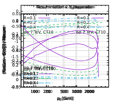
At first sight, this observation is somewhat surprising, insofar as $t$ would appear to be the natural variable for considering small $R$ effects. Part of the explanation is as follows: the $t$ expansion has alternating sign coefficients, at least for the first couple of orders. This means that the NLO ${\cal O}\left(t\right)$ correction (relative to LO) is larger than the overall effect of resummation. The ${\cal O}\left(\alpha_{s}\right)$ correction has the same coefficient as the ${\cal O}\left(t\right)$ correction (modulo an overall normalisation factor of $\frac{1}{2\pi}\ln R_{0}^{2}/R^{2}$). However, $t$ involves the average of the coupling over a range of scales between $p_{t}$ and $Rp_{t}$, which is larger than $\alpha_{s}(p_{t})$. Consequently, the NLO ${\cal O}\left(\alpha_{s}\right)$ term is not as large as the NLO ${\cal O}\left(t\right)$ term, and it overshoots the resummation by less. Though not illustrated in Fig. 23, a similar phenomenon occurs also when comparing to expansions at NNLO.

One should keep in mind that for observables other than the inclusive jet spectrum, it may no longer be true that a $t$ expansion converges more slowly than an $\alpha_{s}$ expansion. Rather, when discussing fixed-order convergence properties compared to full small-$R$ resummation, one should simply be aware that the convergence properties of the $t$ and $\alpha_{s}$ expansions will be sometimes be noticeably different.

Note also that the above discussion holds specifically for the expansion of the LL_R result. As we have seen in section 2.2, NLL_R effects are large and at NNLO are of opposite sign to the LL_R contribution. This further complicates the discussion of the convergence properties of the inclusive jet spectrum.

Appendix B Scale choice beyond leading order

When making fixed-order predictions for the inclusive jet cross section, there are two widely used prescriptions for the choice of a central renormalisation and factorisation scale. One prescription is to use a single scale for the whole event, set by the $p_{t}$ of the hardest jet in the event, $\mu_{0}=p_{t,\max}$. This was adopted, for example, in Ref. Aad:2014vwa . Another prescription is to take instead a different scale for each jet, specifically that jet’s $p_{t}$, $\mu_{0}=p_{t,\text{jet}}$. This was adopted for example in Ref. Abelev:2013fn .

At LO, the two prescriptions give identical results, since there are only two jets in the event and they have the same $p_{t}$. However, starting from NLO the prescriptions can differ substantially. Interestingly, a study of the small-radius limit can provide considerable insight into which choice is more appropriate.

Figure 24: Left: ratio of NLO predictions for the inclusive spectrum when using the per-jet scale choice $\mu_{0}=p_{t,\text{jet}}$ versus the per-event choice $\mu_{0}=p_{t,\max}$. The results are shown as a function of jet $p_{t}$ for three jet radius choices, $R=0.1,0.4$ and $1.0$ and have been obtained with NLOJet++. The bands correspond to the effect of scale variation, where the scales are varied upwards and downwards by a factor of two simultaneously for the numerator and denominator. Right: fraction of the inclusive jet spectrum (for $|y|<0.5$) that comes from jets beyond the two hardest. The 3-jet rate and the overall normalisation are both evaluated at LO.

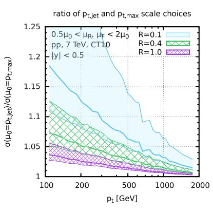
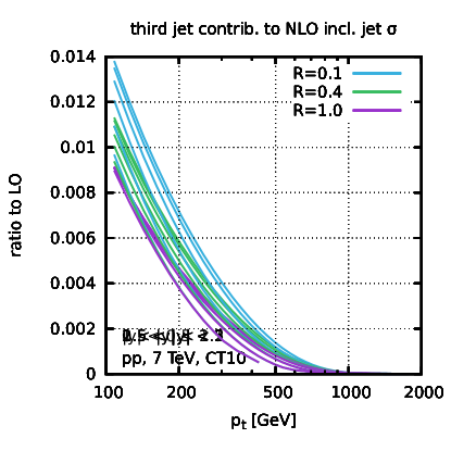
Figure 24 (left) shows the ratio of the NLO result as obtained with $\mu_{0}=p_{t,\text{jet}}$ to that with $\mu_{0}=p_{t,\text{max}}$, as a function of the jet $p_{t}$, for three different jet radii. The main observation is that the $\mu_{0}=p_{t,\text{jet}}$ prescription increases the cross section, especially at small radii: it brings an increase of almost $20\%$ for $R=0.1$ at low $p_{t}$, versus $\lesssim 4\%$ for $R=1.0$ (in both cases for a central scale choice). As we saw in section 4, for reasonably small $R$, the NNLO corrections suppress the cross section. Therefore the choice $\mu_{0}=p_{t,\text{jet}}$ takes us in the wrong direction.

In order to understand this better, it is useful to make a number of observations:

1. For the virtual part of the NLO calculation, the two scale prescriptions give identical results, so the deviation of the ratio from $1$ in Fig. 24 (left) can come only from the real part.

2. The real part itself involves two different pieces: that from binning either of the two leading jets, and that from binning the 3rd jet. The right-hand plot of Fig. 24 shows that the leading-order 3rd-jet contribution is at the level of $1{-}2\%$ of the leading-order dijet result and so it is reasonable to neglect it in our discussion.

3. When a real emission is within an angle $R$ of its nearest other parton, there are only two jets in the event and the two scale-choice prescriptions are identical.

4. Differences between the prescriptions arise when the softest parton falls outside one of the two leading jets. Then one of those jets has a reduced $p_{t}$ and the choice $\mu_{0}=p_{t,\text{jet}}$ gives a smaller scale than $\mu_{0}=p_{t,\text{max}}$. This occurs with a probability that is enhanced by $\ln 1/R$.

5. At $p_{t}\sim 100\,\mathrm{GeV}$, where the effects are largest, renormalisation scale ($\mu_{R}$) variations play a much larger role than factorisation scale ($\mu_{F}$) variations. Therefore a smaller scale translates to a larger value of $\alpha_{s}$ and thus a larger cross section for the real contribution (which is always positive). Consequently, the prescription $\mu_{0}=p_{t,\text{jet}}$ leads to a cross section that is larger than the prescription $\mu_{0}=p_{t,\text{max}}$ and the difference is enhanced by a factor $\ln 1/R$ for small $R$.

This qualitatively explains the behaviour seen in Fig. 24 (left). The $\mu_{0}=p_{t,\text{jet}}$ scale choice introduces a correction that goes in the wrong direction because it leads to a smaller scale (and larger $\alpha_{s}$) for the real part, but without a corresponding modification of the virtual part. Thus it breaks the symmetry between real and virtual corrections.

The above reasoning leads us to prefer the $\mu_{0}=p_{t,\text{max}}^{R=1}$ prescription. To make it a unique event-wide choice, independent of $R$, we define always define $\mu_{0}=p_{t,\text{max}}$ using jets with a radius equal to one, regardless of the $R$ value used in the measurement.

We note that $\mu_{0}=p_{t,\text{max}}$ has a potential linear sensitivity to initial-state radiation, i.e. initial state radiation of transverse momentum $p_{t,i}$ shifts $\mu_{0}$ by an amount $p_{t,i}$. A yet more stable choice might be $\mu_{0}=\frac{1}{2}(p_{t,1}+p_{t,2})$, the average transverse momentum of the two hardest jets (again defined with a radius of one). For this choice, the shift of $\mu_{0}$ would be limited ${\cal O}\left(p_{t,i}^{2}/(p_{t,1}+p_{t,2})\right)$. We leave its study to future work.

Yet another option is the use of MINLO type procedures Hamilton:2012np . For dijet systems, this should be rather similar to $\mu_{0}=\frac{1}{2}(p_{t,1}+p_{t,2})$.

References

- (1) F. Aversa, L. Gonzales, M. Greco, P. Chiappetta and J. P. Guillet, “Jet cone size dependence of inclusive cross-sections to O,” Z. Phys. C 49 (1991) 459.
- (2) F. Aversa, M. Greco, P. Chiappetta and J. P. Guillet, “Jet inclusive production to O : Comparison with data,” Phys. Rev. Lett. 65 (1990) 401.
- (3) J. P. Guillet, “One jet O cross-section: Mass dependence,” Z. Phys. C 51 (1991) 587.
- (4) B. Jager, M. Stratmann and W. Vogelsang, “Single inclusive jet production in polarized collisions at ,” Phys. Rev. D 70 (2004) 034010 [hep-ph/0404057].
- (5) A. Mukherjee and W. Vogelsang, “Jet production in (un)polarized pp collisions: dependence on jet algorithm,” Phys. Rev. D 86 (2012) 094009 [arXiv:1209.1785 [hep-ph]].
- (6) T. Kaufmann, A. Mukherjee and W. Vogelsang, “Next-to-leading Order Calculation for Jets Defined by a Maximized Jet Function,” Phys. Rev. D 91 (2015) 3, 034001 [arXiv:1412.0298 [hep-ph]].
- (7) M. Dasgupta, F. Dreyer, G. P. Salam and G. Soyez, “Small-radius jets to all orders in QCD,” JHEP 1504 (2015) 039 [arXiv:1411.5182 [hep-ph]].
- (8) S. Catani, M. Fontannaz, J. P. .Guillet and E. Pilon, “Isolating Prompt Photons with Narrow Cones,” JHEP 1309 (2013) 007 [arXiv:1306.6498 [hep-ph]].
- (9) S. Alioli and J. R. Walsh, “Jet Veto Clustering Logarithms Beyond Leading Order,” JHEP 1403 (2014) 119 [arXiv:1311.5234(v2) [hep-ph]].
- (10) T. Becher, M. Neubert, L. Rothen and D. Y. Shao, “An Effective Field Theory for Jet Processes,” arXiv:1508.06645 [hep-ph].
- (11) Y. T. Chien, A. Hornig and C. Lee, “A Soft-Collinear Mode for Jet Cross Sections in Soft Collinear Effective Theory,” Phys. Rev. D 93 (2016) 1, 014033 [arXiv:1509.04287 [hep-ph]].
- (12) A. Banfi, F. Caola, F. A. Dreyer, P. F. Monni, G. P. Salam, G. Zanderighi and F. Dulat, “Jet-vetoed Higgs cross section in gluon fusion at N3LO+NNLL with small-R resummation,” arXiv:1511.02886 [hep-ph].
- (13) B. Abelev et al. [ALICE Collaboration], “Measurement of the inclusive differential jet cross section in collisions at TeV,” Phys. Lett. B 722 (2013) 262 [arXiv:1301.3475 [nucl-ex]].
- (14) S. Chatrchyan et al. [CMS Collaboration], “Measurement of the ratio of inclusive jet cross sections using the anti- algorithm with radius parameters and in pp collisions at = 7 TeV,” Phys. Rev. D 90 (2014) 7, 072006 [arXiv:1406.0324 [hep-ex]].
- (15) M. Ploskon [STAR Collaboration], “Inclusive cross section and correlations of fully reconstructed jets in GeV Au+Au and p+p collisions,” Nucl. Phys. A 830 (2009) 255C [arXiv:0908.1799 [nucl-ex]].
- (16) S. Eckweiler, “Measurement of the inclusive jet cross-section in proton-proton collisions at = 7 TeV with the ATLAS detector,” CERN-THESIS-2011-145.
- (17) G. Soyez, “A Simple description of jet cross-section ratios,” Phys. Lett. B 698 (2011) 59 [arXiv:1101.2665 [hep-ph]].
-
(18)
J. Currie, A. Gehrmann-De Ridder, E. W. N. Glover and J. Pires,
“NNLO QCD corrections to jet production at hadron colliders from gluon scattering,”
JHEP 1401 (2014) 110
[arXiv:1310.3993 [hep-ph]];
see also J. Pires, “Future prospects of from jets at the LHC at NNLO”, talk at the Workshop on high-precision measurements: from LHC to FCC-ee, CERN, October 2015, https://indico.cern.ch/event/392530/session/2/contribution/19/attachments/1169760/1688121/pires.pdf - (19) M. Dasgupta, L. Magnea and G. P. Salam, “Non-perturbative QCD effects in jets at hadron colliders,” JHEP 0802 (2008) 055 [arXiv:0712.3014 [hep-ph]].
- (20) T. Sjostrand, S. Mrenna and P. Z. Skands, “PYTHIA 6.4 Physics and Manual,” JHEP 0605 (2006) 026 [hep-ph/0603175].
- (21) T. Sjostrand, S. Mrenna and P. Z. Skands, “A Brief Introduction to PYTHIA 8.1,” Comput. Phys. Commun. 178 (2008) 852 [arXiv:0710.3820 [hep-ph]].
- (22) G. Corcella, I. G. Knowles, G. Marchesini, S. Moretti, K. Odagiri, P. Richardson, M. H. Seymour and B. R. Webber, “HERWIG 6: An Event generator for hadron emission reactions with interfering gluons (including supersymmetric processes),” JHEP 0101 (2001) 010 [hep-ph/0011363].
- (23) G. Corcella, I. G. Knowles, G. Marchesini, S. Moretti, K. Odagiri, P. Richardson, M. H. Seymour and B. R. Webber, “HERWIG 6.5 release note,” hep-ph/0210213.
- (24) M. Bahr et al., “Herwig++ Physics and Manual,” Eur. Phys. J. C 58 (2008) 639 [arXiv:0803.0883 [hep-ph]].
- (25) J. Bellm et al., “Herwig++ 2.7 Release Note,” arXiv:1310.6877 [hep-ph].
- (26) G. Aad et al. [ATLAS Collaboration], “Measurement of the inclusive jet cross-section in proton-proton collisions at TeV using 4.5 fb-1 of data with the ATLAS detector,” JHEP 1502 (2015) 153 [erratum JHEP 1509 (2015) 141] [arXiv:1410.8857 [hep-ex]].
- (27) M. Dasgupta, F. A. Dreyer, G. P. Salam and G. Soyez, http://microjets.hepforge.org.
- (28) R. K. Ellis, W. J. Stirling and B. R. Webber, “QCD and collider physics,” Camb. Monogr. Part. Phys. Nucl. Phys. Cosmol. 8 (1996) 1.
- (29) S. Catani, Y. L. Dokshitzer, M. H. Seymour and B. R. Webber, “Longitudinally invariant clustering algorithms for hadron hadron collisions,” Nucl. Phys. B 406 (1993) 187.
- (30) S. D. Ellis and D. E. Soper, “Successive combination jet algorithm for hadron collisions,” Phys. Rev. D 48 (1993) 3160 [hep-ph/9305266].
- (31) Y. L. Dokshitzer, G. D. Leder, S. Moretti and B. R. Webber, “Better jet clustering algorithms,” JHEP 9708 (1997) 001 [hep-ph/9707323].
- (32) M. Wobisch and T. Wengler, “Hadronization corrections to jet cross-sections in deep inelastic scattering,” In *Hamburg 1998/1999, Monte Carlo generators for HERA physics* 270-279 [hep-ph/9907280].
- (33) M. Cacciari, G. P. Salam and G. Soyez, “The Anti-k(t) jet clustering algorithm,” JHEP 0804 (2008) 063 [arXiv:0802.1189 [hep-ph]].
- (34) G. P. Salam and G. Soyez, “A Practical Seedless Infrared-Safe Cone jet algorithm,” JHEP 0705 (2007) 086 [arXiv:0704.0292 [hep-ph]].
- (35) M. Cacciari, G. P. Salam and G. Soyez, “FastJet User Manual,” Eur. Phys. J. C 72 (2012) 1896 [arXiv:1111.6097 [hep-ph]].
- (36) G. P. Salam and J. Rojo, “A Higher Order Perturbative Parton Evolution Toolkit (HOPPET),” Comput. Phys. Commun. 180 (2009) 120 [arXiv:0804.3755 [hep-ph]].
- (37) Z. Nagy, “Next-to-leading order calculation of three jet observables in hadron hadron collision,” Phys. Rev. D 68 (2003) 094002 [hep-ph/0307268].
- (38) H. L. Lai, M. Guzzi, J. Huston, Z. Li, P. M. Nadolsky, J. Pumplin and C.-P. Yuan, “New parton distributions for collider physics,” Phys. Rev. D 82 (2010) 074024 [arXiv:1007.2241 [hep-ph]].
- (39) A. Gehrmann-De Ridder, T. Gehrmann, E. W. N. Glover, A. Huss and T. A. Morgan, “NNLO QCD corrections for Z boson plus jet production,” arXiv:1601.04569 [hep-ph].
- (40) I. W. Stewart and F. J. Tackmann, “Theory Uncertainties for Higgs and Other Searches Using Jet Bins,” Phys. Rev. D 85 (2012) 034011 [arXiv:1107.2117 [hep-ph]].
- (41) A. Banfi, G. P. Salam and G. Zanderighi, “NLL+NNLO predictions for jet-veto efficiencies in Higgs-boson and Drell-Yan production,” JHEP 1206 (2012) 159 [arXiv:1203.5773 [hep-ph]].
- (42) D. de Florian, P. Hinderer, A. Mukherjee, F. Ringer and W. Vogelsang, “Approximate next-to-next-to-leading order corrections to hadronic jet production,” Phys. Rev. Lett. 112 (2014) 082001 [arXiv:1310.7192 [hep-ph]].
- (43) S. Alioli, K. Hamilton, P. Nason, C. Oleari and E. Re, “Jet pair production in POWHEG,” JHEP 1104 (2011) 081 [arXiv:1012.3380 [hep-ph]].
- (44) R. Corke and T. Sjostrand, “Interleaved Parton Showers and Tuning Prospects,” JHEP 1103 (2011) 032 [arXiv:1011.1759 [hep-ph]].
- (45) P. Z. Skands, “Tuning Monte Carlo Generators: The Perugia Tunes,” Phys. Rev. D 82 (2010) 074018 [arXiv:1005.3457 [hep-ph]].
- (46) [ATLAS Collaboration], “New ATLAS event generator tunes to 2010 data,” ATL-PHYS-PUB-2011-008, ATL-COM-PHYS-2011-329.
- (47) G. Aad et al. [ATLAS Collaboration], “Measurement of inclusive jet and dijet production in collisions at TeV using the ATLAS detector,” Phys. Rev. D 86 (2012) 014022 [arXiv:1112.6297 [hep-ex]].
- (48) Y. L. Dokshitzer and B. R. Webber, “Calculation of power corrections to hadronic event shapes,” Phys. Lett. B 352 (1995) 451 [hep-ph/9504219].
- (49) G. P. Korchemsky and G. F. Sterman, “Nonperturbative corrections in resummed cross-sections,” Nucl. Phys. B 437 (1995) 415 [hep-ph/9411211].
- (50) M. H. Seymour, “Jet shapes in hadron collisions: Higher orders, resummation and hadronization,” Nucl. Phys. B 513 (1998) 269 [hep-ph/9707338].
- (51) M. Cacciari, G. P. Salam and G. Soyez, “The Catchment Area of Jets,” JHEP 0804 (2008) 005 [arXiv:0802.1188 [hep-ph]].
- (52) Y. L. Dokshitzer, G. Marchesini and B. R. Webber, “Dispersive approach to power behaved contributions in QCD hard processes,” Nucl. Phys. B 469 (1996) 93 [hep-ph/9512336].
- (53) P. Skands, S. Carrazza and J. Rojo, “Tuning PYTHIA 8.1: the Monash 2013 Tune,” Eur. Phys. J. C 74 (2014) 8, 3024 [arXiv:1404.5630 [hep-ph]].
- (54) R. Field, “Early LHC Underlying Event Data - Findings and Surprises,” arXiv:1010.3558 [hep-ph].
- (55) B. Cooper, J. Katzy, M. L. Mangano, A. Messina, L. Mijovic and P. Skands, “Importance of a consistent choice of in the matching of AlpGen and Pythia,” Eur. Phys. J. C 72 (2012) 2078 [arXiv:1109.5295 [hep-ph]].
- (56) G. P. Salam and D. Wicke, “Hadron masses and power corrections to event shapes,” JHEP 0105 (2001) 061 [hep-ph/0102343].
- (57) V. Mateu, I. W. Stewart and J. Thaler, “Power Corrections to Event Shapes with Mass-Dependent Operators,” Phys. Rev. D 87 (2013) 1, 014025 [arXiv:1209.3781 [hep-ph]].
- (58) G. Aad et al. [ATLAS Collaboration], “Study of Jet Shapes in Inclusive Jet Production in Collisions at TeV using the ATLAS Detector,” Phys. Rev. D 83 (2011) 052003 [arXiv:1101.0070 [hep-ex]].
- (59) S. Chatrchyan et al. [CMS Collaboration], “Shape, Transverse Size, and Charged Hadron Multiplicity of Jets in pp Collisions at 7 TeV,” JHEP 1206 (2012) 160 [arXiv:1204.3170 [hep-ex]].
- (60) G. P. Korchemsky and G. F. Sterman, “Power corrections to event shapes and factorization,” Nucl. Phys. B 555 (1999) 335 [hep-ph/9902341].
- (61) S. Gieseke, C. Rohr and A. Siodmok, “Colour reconnections in Herwig++,” Eur. Phys. J. C 72 (2012) 2225 [arXiv:1206.0041 [hep-ph]].
- (62) J. Collins and J. W. Qiu, “ factorization is violated in production of high-transverse-momentum particles in hadron-hadron collisions,” Phys. Rev. D 75 (2007) 114014 [arXiv:0705.2141 [hep-ph]].
- (63) S. Chatrchyan et al. [CMS Collaboration], “Measurements of differential jet cross sections in proton-proton collisions at TeV with the CMS detector,” Phys. Rev. D 87 (2013) 11, 112002 [arXiv:1212.6660 [hep-ex]].
- (64) V. Khachatryan et al. [CMS Collaboration], “Measurement of the inclusive jet cross section in pp collisions at TeV,” arXiv:1512.06212 [hep-ex].
- (65) J. Gao et al., “CT10 next-to-next-to-leading order global analysis of QCD,” Phys. Rev. D 89 (2014) 3, 033009 [arXiv:1302.6246 [hep-ph]].
- (66) S. Dulat et al., “The CT14 Global Analysis of Quantum Chromodynamics,” arXiv:1506.07443 [hep-ph].
- (67) A. D. Martin, W. J. Stirling, R. S. Thorne and G. Watt, “Parton distributions for the LHC,” Eur. Phys. J. C 63 (2009) 189 [arXiv:0901.0002 [hep-ph]].
- (68) L. A. Harland-Lang, A. D. Martin, P. Motylinski and R. S. Thorne, “Parton distributions in the LHC era: MMHT 2014 PDFs,” Eur. Phys. J. C 75 (2015) 5, 204 [arXiv:1412.3989 [hep-ph]].
- (69) R. D. Ball et al. [NNPDF Collaboration], “Parton distributions for the LHC Run II,” JHEP 1504 (2015) 040 [arXiv:1410.8849 [hep-ph]].
- (70) S. Dittmaier, A. Huss and C. Speckner, “Weak radiative corrections to dijet production at hadron colliders,” JHEP 1211 (2012) 095 [arXiv:1210.0438 [hep-ph]].
- (71) U. Baur, “Weak Boson Emission in Hadron Collider Processes,” Phys. Rev. D 75 (2007) 013005 [hep-ph/0611241].
- (72) N. Méric, “Etude théorique et expérimentale des corrections électrofaibles au processus de production inclusive de jets. Développement de méthodes de détection de topologies extrêmes,” CERN-THESIS-2013-358, https://tel.archives-ouvertes.fr/tel-00959427/
- (73) ATLAS Collaboration, HepData entry corresponding to Ref.Aad:2014vwa , http://hepdata.cedar.ac.uk/view/ins1325553.
- (74) S. D. Ellis, Z. Kunszt and D. E. Soper, “Two jet production in hadron collisions at order in QCD,” Phys. Rev. Lett. 69 (1992) 1496.
- (75) K. Hamilton, P. Nason and G. Zanderighi, “MINLO: Multi-Scale Improved NLO,” JHEP 1210 (2012) 155 [arXiv:1206.3572 [hep-ph]].