Young and middle age pulsar light-curve morphology: Comparison of Fermi observations with $\gamma$-ray and radio emission geometries

Thanks to the huge amount of $\gamma$-ray pulsar photons collected by the Fermi Large Area Telescope since its launch in June 2008, it is now possible to constrain $\gamma$-ray geometrical models by comparing simulated and observed light-curve morphological characteristics. We assumed vacuum-retarded dipole (VRD) pulsar magnetic field and tested simulated and observed morphological light-curve characteristics in the framework of two pole emission geometries, Polar Cap (PC) and Slot Gap (SG), and one pole emission geometries, traditional Outer Gap (OG) and One Pole Caustic (OPC). Radio core plus cone emission was assumed for the pulsar of the simulated sample. We compared simulated and observed recurrence of class shapes and peak multiplicity, peak separation, radio-lag distributions, and trends of peak separation and radio lag as a function of observable and non-observable pulsar parameters. We studied how pulsar morphological characteristics change in multi-dimensional observable and non-observable pulsar parameter space.

The PC model gives the poorest description of the LAT pulsar light-curve morphology. The OPC best explains both the observed $\gamma$-ray peak multiplicity and shape classes. The OPC and SG models describe the observed $\gamma$-ray peak-separation distribution for low- and high-peak separations, respectively. This suggests that the OPC geometry best explains the single-peak structure but does not manage to describe the widely separated peaks predicted in the framework of the SG model as the emission from the two magnetic hemispheres. The OPC radio-lag distribution shows higher agreement with observations suggesting that assuming polar radio emission, the $\gamma$-ray emission regions are likely to be located in the outer magnetosphere. Alternatively, the radio emission altitude could be higher that we assumed. We compared simulated non-observable parameters with the same parameters estimated for LAT pulsars in the framework of the same models. The larger agreement between simulated and LAT estimations in the framework of the OPC suggests that the OPC model best predicts the observed variety of profile shapes. The larger agreement obtained between observations and the OPC model predictions jointly with the need to explain the abundant 0.5 separated peaks with two-pole emission geometries, calls for thin OPC gaps to explain the single-peak geometry but highlights the need of two-pole caustic emission geometry to explain widely separated peaks.

1 Introduction

	PC	SG	OG	OPC	Radio
$\sigma_{\nu}$	0.005	0.9	0.2	0.2	0.2
$\delta\sigma_{\nu}$	0.001	0.1	0.01	0.01	0.01
$Th_{0}$	0.02	0.05	0.03	0.03	0.04
$Th_{mx-mn}$	0.001	0.15	0.03	0.03	0.01
$W_{H}$	$W(0.50(\max-\min))$	$W(\min+0.50(\max-\min))$	$W(0.50(\max-\min))$	$W(0.50(\max-\min))$	$W(0.50(\max-\min))$
$W_{B}$	$W(0)$	$W(\min+0.15(\max-\min))$	$W(0)$	$W(0)$	$W(0)$

Table 1: Values adopted in each model for the light-curve smoothing $\sigma_{\nu}$ and $\delta\sigma_{\nu}$, the zero threshold $Th_{0}$ and maximum-minimum detection threshold $Th_{mx-mn}$, and the peak widths, $W_{H}$ and $W_{B}$ for modelled $\gamma$-ray and radio light curves. The parameters $W_{H}$ and $W_{B}$ are expressed as the width $W$ of the peak measured at a certain fraction $x$ of the peak maximum, $W(x)$. The terms “$\min$” and “$\max$” refer to light-curve minimum and maximum, respectively. All values are given in phase units.

The successful launch of the Fermi Gamma-ray space telescope satellite (hereafter Fermi) in June 2008 represents a milestone in pulsar astrophysics research. Owing to the observations performed with its main instrument, the Large Area Telescope (LAT), Fermi increased the number of known young or middle-aged $\gamma$-rays pulsars by a factor $\sim$30, discovered the new category of $\gamma$-ray millisecond pulsars, and obtained unprecedented high quality light curves for the major part of the observed objects.

The increasing number of $\gamma$-ray pulsars detected by Fermi, which is now second just to the number of pulsars detected at radio wavelengths, offered the possibility, for the first time with high statistics, of studying the collective properties of the $\gamma$-ray pulsar population and to compare them with model predictions (e.g. pulsar population syntheses; Watters & Romani (2011); Takata et al. (2011); light-curve fitting and morphology analysis; Watters et al. (2009); Romani & Watters (2010)). Pierbattista (2010) performed a comprehensive study of the Fermi $\gamma$-ray pulsars detected by LAT during the first year of observations (The first Fermi large-area telescope catalogue of $\gamma$-ray pulsars, Abdo et al., 2010, hereafter PSRCAT1). Pierbattista (2010) tested radiative and geometrical models against the observations according to three different approaches: a neutron star (NS) population synthesis to compare collective radiative properties of observed and simulated pulsar populations; a simulation of the observed pulsar emission patterns to estimate non-observable pulsar parameters and to study their relationship with observable pulsar characteristics in the framework of different emission geometries; and a comparison of simulated and observed light-curve morphological characteristics in the framework of different emission geometries. The population synthesis and the estimate of non-observable LAT pulsar parameters have been presented in Pierbattista et al. (2012; hereafter PIERBA12) and by Pierbattista et al. (2015; hereafter PIERBA15) , respectively.

PIERBA12 synthesised a NS population, evolved this population in the galactic gravitational potential assuming a supernova kick velocity and birth space distribution, and computed, for each NS of the sample, $\gamma$-ray and radio radiation powers and light curves according to radiative $\gamma$-ray models and a radio model. The implemented radiative $\gamma$-ray models are: the Polar Cap model (PC; Muslimov & Harding, 2003), Slot Gap model (SG; Muslimov & Harding, 2004), Outer Gap model (OG; Cheng et al., 2000), and the One Pole Caustic model (OPC; Romani & Watters, 2010; Watters et al., 2009), which is an alternative formulation of the OG that only differs in the computation of radiative power and width of the emission region. In the OPC model, both gap width and gap-width luminosity have been set to reproduce the relation $L_{\gamma}\propto\dot{E}^{0.5}$ observed in PSRCAT1; since the gap width is assumed equal to the $\gamma$-ray efficiency, $w_{\mathrm{OPC}}\propto\dot{E}^{-0.5}$, the luminosity must follow $L_{\gamma}=\dot{E}w_{\mathrm{OPC}}$. Because of that, the OPC cannot be considered a full physical model like PC, SG, and OG, but a phenomenological formulation of the OG, built in to reproduce the observations. Each pulsar radio luminosity has been computed according to a radio core plus cone model, following the prescriptions from Gonthier et al. (2004), Story et al. (2007), and Harding et al. (2007). Simulation details can be found in PIERBA12. The $\gamma$-ray and radio light curves of the simulated pulsar have been obtained according to the geometrical model from Dyks et al. (2004). Under the assumption that $\gamma$-ray and radio photons are emitted tangent to the poloidal magnetic field line in the reference frame instantaneously corotating with the pulsar, $\gamma$-ray and radio light curves have been computed by assuming location and size of the emission region in the framework of each $\gamma$-ray model and radio model. The directions of the photons generated at the emission point have been computed as described in Bai & Spitkovsky (2010). The complete description of the method used to simulate $\gamma$-ray and radio light curves of the observed pulsars can be found in PIERBA15.

Pierbattista et al. (2015) simulated the emission pattern of the young or middle-aged LAT $\gamma$-ray pulsars detected after three years of observations and published in the second LAT $\gamma$-ray pulsars catalogue (Abdo et al., 2013, hereafter PSRCAT2), and used them to fit the observed profiles. The LAT pulsar emission patterns were computed in the framework of the very same radiative models implemented by PIERBA12, namely PC, SG, OG, OPC, and radio core plus cone, and by assuming emission geometry according to Dyks et al. (2004). For each LAT pulsar and each model, $\gamma$-ray and radio light curves were computed for a grid of values of magnetic obliquity $\alpha$ (angle between the pulsar magnetic and rotational axes) and observer line-of-sight $\zeta$ (angle between the rotational axis and the direction of the observer), both stepped every 5^∘ in the interval 1 to 90, for the actual pulsar spin period (P), and for the magnetic field (B) and width of the emission gap region (W) computed as described in PIERBA12. A best-fit light curve with relative best-fit parameters, $\alpha$, $\zeta$, and W, were found in the framework of each model and for each pulsar by fitting the observed light curves with the emission patterns through a maximum likelihood criterion.

The aim of this paper is to further develop and improve the light-curve morphological analysis implemented by Pierbattista (2010) by testing the PC, SG, OG, OPC, and radio core plus cone emission geometries against the young and middle-aged pulsar sample published in PSRCAT2. We computed a series of light-curve morphological characteristics, namely $\gamma$-ray and radio peak numbers, their phase separation, the lag between the occurrence of $\gamma$-ray and radio peaks in radio loud (RL) pulsars, among others, for both observed and simulated light curves and within each model. The simulated pulsar light curves are those synthesised by PIERBA12 in the framework of PC, SG, OG, OPC, and radio core plus cone models by assuming emission geometry from Dyks et al. (2004). We build a light-curve shape classifications according to the recurrence of the morphological characteristics in observed and simulated profiles and compared simulated and observed shape classifications in the framework of each model. We compared observed and simulated distributions of morphological characteristics as a function of observable and non-observable pulsar parameters. The non-observable pulsar parameters, namely $\alpha$, $\zeta$, and $\gamma$-ray beaming factor $f_{\Omega}$, are those estimated by PIERBA15 in the framework of the implemented emission geometries. We obtained constraints on the emission geometry that best explains the observations.

The outline of this paper is as follows. In Section 2 we characterise both simulated and observed $\gamma$-ray pulsar samples. In Section 3 we describe the method used to classify simulated and observed pulsars and compare simulated and observed $\gamma$-ray and the peak multiplicity of radio light curves. In Section 4 we describe the criteria used to measure the light-curve morphological characteristics for both observed and simulated objects and compare observed and simulated distributions and trends of observable and non-observable/estimated pulsar parameters. Section 5 shows the $\gamma$-ray peak multiplicity and peak separation in the $(\alpha,\zeta)$ plane for both simulated and observed pulsars (estimated values). Section 6 summarises the results.

In Appendix A templates of the $\gamma$-ray and radio shape classes defined in Section 3 are shown in the framework of each model. In Appendix B the pulsar $\gamma$-ray and radio emission patterns are shown to ease the interpretation of the results. In Appendix C we compare the recurrence of simulated and observed $\gamma$-ray light-curve multiplicity for radio quiet and radio loud pulsars and of simulated and observed $\gamma$-ray and radio shape classes. In Appendix D we give exhaustive maps showing the $\gamma$-ray peak multiplicity and $\gamma$-ray peak separation as a function of the spin period (PC) and width of the acceleration gap (SG, OG, and OPC) in Figure 19 and 20, respectively. Appendix E.1 describe the one-and two-dimensional Kolmogorov-Smirnov (KS) tests used to quantify the agreement between observed and simulated distributions.

2 Data selection and simulated sample

Figure 1: Examples of light-curve classification criteria used to classify the simulated light curves. From top to bottom are shown: PC or radio bump light curve; PC or radio two peaks light curve; SG double plus single peak light curve; OG or OPC triple peak light curve.

We have analysed 77 young or middle-aged pulsars listed in PSRCAT2. We obtained their $\gamma$-ray and radio light curves from the LAT catalogue data products public link. We built each Fermi $\gamma$-ray pulsar light curve with 3 years of LAT observations from 2008 August 4 to 2011 August 4 selecting only photons with energy larger than 100 MeV and belonging to the source class, as defined in the P7_V6 instrument response function. We obtained the Fermi $\gamma$-ray light curves as weighted light curves where each photon is characterised by its probability to belong to the pulsar with the photon weights following the Gaussian probability distribution (PSRCAT2). We built the radio light curves of the analysed RL pulsars from observations mainly performed at 1400 MHz by the radio telescopes operating within the Fermi Pulsar Search Consortium (PSC; Ray et al., 2012) and the Fermi Pulsar Timing Consortium (PTC; Smith et al., 2008), namely the Green Bank Telescope (GBT), Parkes Telescope, Nançay Radio Telescope (NRT), Arecibo Telescope, the Lovell Telescope at Jodrell Bank, and the Westerbork Synthesis Radio Telescope (Smith et al., 2008). See PSRCAT2 for details about how the $\gamma$-ray and radio light curves were obtained.

The simulated radio and $\gamma$-ray light curves used in this paper are those obtained within the population synthesis from PIERBA12. Those authors classified the simulated NSs as radio quiet (RQ) or radio loud (RL) $\gamma$-ray pulsars according to emission-geometry visibility criteria ($\gamma$-ray and radio beam orientations) and according to the $\gamma$-ray flux and radio flux sensitivity. The emission-geometry visibility criteria classify a NS as a RL or RQ pulsar when the observer line of sight simultaneously intersects $\gamma$-ray and radio emission beams or just the $\gamma$-ray emission beam, respectively. The $\gamma$-ray and radio flux sensitivity criteria adopted in PIERBA12 are scaled up to three years from one year of $\gamma$-ray LAT sensitivity and on the sensitivity of ten radio surveys. Different $\gamma$-ray sensitivities were used for pulsars discovered through blind search and for pulsar detected using a timing solution known from radio observations. The radio sensitivity for RL LAT pulsars has been obtained by recomputing the survey parameters of the ten radio surveys covering the largest possible sky surface and for which the survey parameters were known with high accuracy. Details about $\gamma$-ray and radio visibility computation can be found in PIERBA12.

In this paper we make use of the three-year LAT $\gamma$-ray pulsar sensitivity and on updated radio observations of the radio loud LAT pulsars. Since the morphological classification of the simulated light curves does not show significant variations between the whole simulated population and its visible subsample (as we show in section 3.2), we compare the LAT morphological characteristics with the morphological characteristics of all simulated pulsars classified as visible according to emission geometry visibility criteria only.

3 Shape classification of observed and simulated light curves

3.1 Method

	PC		SG
Shape Class	$(N_{E-W},Pk,Mn)$	Peak Width Condition	$(N_{E-W},Pk,Mn)$	Peak Width Condition
1- Bump	(1,1,0)	$W_{B}\geq 0.40$ & $HL_{R}\geq 0.50$	(1,1,0/1/2)	$W_{B}\geq 0.35$ & $HL_{R}\geq 0.50$
2- Sharp	(1,1,0)	$W_{B}<0.40$ & $HL_{R}<0.50$	(1,1,0/1/2)	$W_{B}<0.35$
3- Shoulder	none	/	(1,1,0/1/2)	$W_{B}\geq 0.35$ & $HL_{R}\geq 0.42$
4- Two	(1,2,0)	/	none	/
5- Double	(1,2,1)	/	(1,2,2/3)	/
6- Double+Single	(2,3,1)	/	(1,2,3)	/
7- Triple/Three	none	/	none	/
8- Two double	(2,4,2)	/	(1,4,4)	/

	OG/OPC		$\gamma$-ray LAT
Shape Class	$(N_{E-W},Pk,Mn)$	Peak Width Condition	$(N_{E-W},Pk,Mn)$	Peak Width Condition
1- Bump	(1,1,0)	$W_{B}\geq 0.20$ & $HL_{R}\geq 0.45$	(1,1,x)	$W_{B}\geq 0.25$ & $HL_{R}\geq 0.40$
2- Sharp	(1,1,0)	$W_{B}<0.10$ & $HL_{R}<0.45$	(1,1,x)	$W_{B}\geq 0.25$ & $HL_{R}\geq 0.40$
3- Shoulder	(1,1,0)	$W_{B}\geq 0.10$ & $HL_{R}<0.45$	(1,1,x)	$W_{B}\geq 0.25$ & $HL_{R}<0.40$
4- Two	(2,2,0)	/	(2,2,x)	/
5- Double	(1,2,0/1/2)	/	(1,2,x)	/
6- Double+Single	none	/	(2,3,x)	/
7- Triple	(1,3,1/2)	/	(1/3,3,x)	/
8- Two double	(1,4,3)	/	(x,4,x)	/

Table 2: Assignation of the $\gamma$-ray light-curve shape classes according to a different set of light-curve morphological characteristics for PC and SG simulated profiles (top table) and OG/OPC simulated profiles and $\gamma$-ray LAT profiles (bottom table). ‘None’ in correspondence of a shape class for a particular model, indicates that this light-curve shape is not observed in the framework of this model. The ‘Peak Width Condition’ was uniquely used to discriminate between ‘Bump’ and ‘Sharp’ single-peak light curves. All values are given in phase units. Light-curve shape templates for the listed shape classes are shown in Table 7.

We defined a number of light-curve morphological characteristics and assigned shape classes to both simulated and observed light curves according to the recurrence of those characteristics in the analysed profiles. They are:

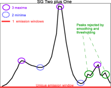
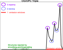
• The number of light-curve phase windows with non-zero emission, $N_{E-W}$, defined as the number of contiguous phase intervals in the analysed light curves that show non-zero emission (see the second and fourth panel of Figure 1 for examples of two and one non-zero emission windows, respectively);

• The number of light-curve peaks, $Pk$ (defined as described in Section 3.1.1 and 3.1.2);

• The number light-curve minima, $Mn$ (defined as described in Section 3.1.1 and 3.1.2);

• The peak full width half maximum, $W_{H}$, and the width at the base of the peak, $W_{B}$, for single peak light curves, both expressed in pulse-phase units. Because of the differences in the off-peak emission predicted by the different models and in the observed light curves, both $W_{H}$ and $W_{B}$ values have been optimised in the framework of each model and for observed profiles. The adopted values for $\gamma$-ray and radio light curves, both simulated and observed, are given in Table 1. An example of $W_{H}$ and $W_{B}$ is shown in the top panel of Figure 1.

  We used $W_{H}$ and $W_{B}$ to define a high-to-low peak width ratio, $HL_{R}=W_{H}/W_{B}$. $HL_{R}$ close to 0 indicates a peak that gets rapidly pointed while $HL_{R}$ close to 1 indicates a peak with a more constant width along its vertical extension. The parameter $HL_{R}$ is used for the classification of the different kinds of single-peak light curves.

Examples of the light-curve maxima, minima, single-peak widths, and non-zero emission windows are shown, for each model, in Figure 1 while the shape classes used to classify $\gamma$-ray and radio light curves are shown in Tables 6 and 7, respectively. The listed morphological characteristics were computed for observed and simulated light curves according to different criteria.

3.1.1 LAT $\gamma$-ray and radio light curves

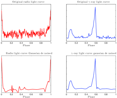
The $\gamma$-ray and radio observed light curves are affected by observational noise that does not allow a clear identification of the light-curve shape morphology and must be removed before the analysis. Both $\gamma$-ray and radio light curves of LAT pulsars have been de-noised using a wavelet transform with an iterative multi-scale thresholding algorithm and assuming Gaussian noise (Starck et al., 2006). We chose Gaussian noise because the statistics of the weighted $\gamma$-ray photons follows a Gaussian distribution (PSRCAT2) and the radio light curves are well described by Gaussian statistics. Examples of the wavelet de-noising of $\gamma$-ray and radio LAT light curves for pulsar J0205+6449 are shown in Figure 2 left (red) and right (blue) panels, respectively.

The $\gamma$-ray light curve of LAT pulsars have been classified by adopting the very same peak multiplicity assigned by PSRCAT2 while the radio light curves of LAT pulsars have been classified on the basis of the analysis of the de-noised light curves. The de-noised $\gamma$-ray or radio light curves also allow us to highlight the presence of an eventual emission bridge between the peaks, which are fundamental for the peak-separation computation (see Section 4).

Figure 2: Examples of the wavelet Gaussian de-noising method used to classify the LAT pulsar light curves. The de-noising of radio and $\gamma$-ray light curves of pulsar J0205$-$6449 are shown on the left (red) and right (blue) panels, respectively.

3.1.2 Simulated $\gamma$-ray and radio light curves

The simulated light curves are characterised by computational fluctuations that affect the light-curve shape as real noise. The light curves of simulated pulsars were computed using the geometrical model from Dyks et al. (2004). In the algorithm that implements the Dyks et al. (2004) model, the number of magnetic field lines where particles are accelerated and $\gamma$-rays are produced is an input parameter; a large magnetic field-line number yields smooth light curves with low computational fluctuations in a computational time that is potentially prohibitive, while a low magnetic field-line density speeds up the computation but generates light curves with a critical computational fluctuations. We chose a magnetic field line number optimised to have a reasonable computational time and moderated computational fluctuations and we reduced the computational fluctuations by smoothing all simulated light curves using a Gaussian filter. The smoothing consisted in computing the fast Fourier transform (FFT) of a Gaussian function with standard deviation $\sigma_{\nu}$ and of the simulated light curve, convolving the two FFTs, and evaluating the inverse FFT of the convolved function. The result is a light curve with all fluctuations of frequency $\sigma_{\nu}$ smoothed. Since each model shows different computational noise, $\sigma_{\nu}$ was optimised in the framework of each model and for $\gamma$-ray and radio observed profiles. They are listed in Table 1.

	Radio Core plus cone / Radio LAT
Shape Class	$(N_{E-W},Pk,Mn)$	Peak Width Condition
1- Bump	(1,1,0/1)	$W_{B}\geq 0.25$ & $HL_{R}\geq 0.50$
2- Sharp	(1,1,0/1)	$W_{B}<0.25$ & $HL_{R}<0.50$
3- Two	(2,2,0/1)	/
4- Double	(1,2,1)	/
5- Double+Single	(2,3,1)	/
6- Two double	(2,4,2)/(4,4,0)	/
7- Triple	(1,3,2)	/
8- Three	(3,3,0)	/
9- Two triple	(2,6,4)	/

Table 3: Assignation of the radio light-curve shape classes according to a different set of light-curve morphological parameters for radio core plus cone simulated light curves and for observed radio light curves. The “Peak Width Condition” was uniquely used to discriminate between “Bump” and “Sharp” single-peak light curves. All width values are given in phase units. Light-curve shape templates for the listed shape classes are shown in Table 7.

The smoothed light curve is then analysed by the analysis script that detects and computes the morphological light-curve characteristics $N_{E-W}$, $Pk$, $Mn$, $W_{H}$, $W_{B}$, and $HL_{R}$. In some cases the main light-curve peak is comparable to the computational fluctuations and the smoothing procedure could modify the peak shape. Moreover, some light curves are characterised by high off-pulse emission that does not allow a clear identification of the light-curve emission windows $N_{E-W}$ (see Figure 1). In order to recognise computational noise maxima from light-curve peaks and not account for the off-peak emission in the number of emission-windows $N_{E-W}$, we defined two threshold criteria. The first criterion consists in placing at zero all light-curve intensities lower than a threshold value $Th_{0}$, usually few percent of the absolute light-curve maximum, which is different for each model. The second criterion consist in defining a maximum-to-minimum detection threshold $Th_{mx-mn}$ so that a light-curve maximum is classified as a peak only if the difference between its intensity and the intensity of the previous minimum is larger than the threshold value $Th_{mx-mn}$, which is different for each model (Figure 1 third panel). The definition of $Th_{0}$ and $Th_{mx-mn}$ for $\gamma$-ray and radio light curves is given in Table 1.

The association between the morphological parameters $N_{E-W}$, $Pk$, $Mn$, $W_{H}$, $W_{B}$, and $HL_{R}$ and the $\gamma$-ray and radio shape classes are shown in Tables 2 and 3, respectively while templates of the correspondent light-curve shapes in the framework of each model are shown in Tables 6 and 7. If the number of light-curve phase windows, the number of peaks, and the number of minima, ($N_{E-W}$, $Pk$, $Mn$), detected by the analysis script in a light curve do not correspond to any shape class listed in Tables 2 and 3, the light curve is tagged as unclassified and the smoothing procedure is repeated by increasing $\sigma_{\nu}$ of a $\delta\sigma_{\nu}$. The re-smoothing of the analysed light curve is a procedure that is iterated by increasing $\sigma_{\nu}$ of a $\delta\sigma_{\nu}$ at each iteration up to a sure identification of the analysed profile. The increasing smoothing factors $\delta\sigma_{\nu}$ were optimised in the framework of each model and are listed in Table 1.

We built the $\gamma$-ray and radio light-curve shape classifications described in Tables 2 and 3 by merging all shape classes obtained in the framework of all observed and simulated $\gamma$-ray light curves and observed and simulated radio light curves, respectively. This explains why some shape classes are not observed in the framework of a particular model.

Figure 3: Recurrence of the shape classes described in Tables 2 and 3 and shown in Tables 6 and 7 for the $\gamma$-ray pulsars (top panels), radio pulsars (bottom panel), and each model for the whole simulated pulsar population and its visible subsample, as synthesised by Pierbattista et al. (2012).

3.2 Shape classification and multiplicity: Comparison of model and observations

	PC		SG		OG		OPC
	$D$	$p_{\mathrm{value}}$ [%]	$D$	$p_{\mathrm{value}}$ [%]	$D$	$p_{\mathrm{value}}$ [%]	$D$	$p_{\mathrm{value}}$ [%]
Fig. 4: $\gamma$-ray peak multiplicity	0.66	1e-28	0.51	7e-16	gray!300.32	gray!302e-5	gray!600.12	gray!6023.3
Fig. 5-left: $\Delta_{\gamma}$ distribution	0.42	2e-8	gray!600.18	gray!602.5	0.54	5e-15	gray!300.29	gray!303e-3
Fig. 5-right: $\Delta_{\mathrm{Radio}}$ distribution	gray!600.19	gray!6057	gray!300.21	gray!3046	0.52	3e-2	0.37	2.6
Fig. 6: $\delta$ distribution	0.81	1e-5	0.50	2e-7	gray!300.39	gray!304e-4	gray!600.22	gray!602.7

Table 4: Two-sample Kolmogorov-Smirnov statistics (2KS) and relative $p_{\mathrm{value}}$ between observed and simulated one-dimensional distributions shown in Figures 4 to 6 for each model. The 2KS statistics $D$ ranges between 0 and 1 for distributions showing total agreement and total disagreement, respectively. The $p_{\mathrm{value}}$ is the probability to obtain the observed $D$ value under the assumption that the two distributions are obtained from the same distribution (null hypothesis). This is equivalent to rejecting the null hypothesis at a confidence level of 100-($p_{\mathrm{value}}$)%. The 2KS test is described in Section E. The $D$ and $p_{\mathrm{value}}$ parameters relative to the first and second most consistent distributions are highlighted in dark grey and light grey cells, respectively.

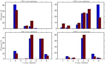
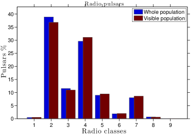
Figure 3 shows the recurrence of $\gamma$-ray and radio shape classes described in Tables 6 and 7 respectively, for the whole simulated population synthesised by PIERBA12 and its visible subsample. The recurrence of each shape class does not change considerably from the whole population to its visible subsample showing that there are no important selection effects due to light-curve shapes. The most pronounced discrepancies are observed within the PC model where the visible subsample shows a lack of sharp peaks (shape class 2) and an excess of double peaks (shape class 4) and in the SG model where the double plus single peak (shape class 8) is less recurrent among visible objects while all other classes are more populated in the whole population. This is confirmed by KS statistics between total and visible subsample distributions of 0.19, 0.21, 0.05, 0.10, and 0.03 for PC, SG, OG, OPC, and radio models, respectively, with the KS statistics ranging from 0 for total agreement to 1 for total disagreement (see Appendix E for details). The consistency between the shape class recurrences in the whole simulated population and its visible subsample allows us to compare the collective properties of the whole simulated population by Pierbattista et al. (2012) with the same properties of the observed pulsar population.

We define the light-curve-peak multiplicity as the number of peaks detected in the radio or $\gamma$-ray light curve according to the method described in Section 3. The $\gamma$-ray and radio light curves multiplicities are associated with each shape class as indicated in Tables 6 and 7, respectively. Figure 4 compares the observed and simulated peak multiplicity distributions for the implemented $\gamma$-ray emission geometries.

Figure 4: Recurrence of $\gamma$-ray peak multiplicity for the simulated (grey) and LAT (red) $\gamma$-ray pulsar populations and each model. 1s refers to one peak with shoulder class 3 in Table 6.

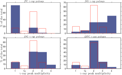
The statistical agreement between observed and simulated $\gamma$-ray peak multiplicity distributions was computed by performing the two-sample Kolmogorov-Smirnov (2KS). Table 4 list the 2KS test results and suggests that the outer magnetosphere models, OG and OPC, best explain the observations, with the OPC prediction showing the highest agreement with observations. The SG model predicts too many high-multiplicity profiles and too few double-peaked profiles. The PC model completely fails to explain the observed multiplicities.

The comparison of simulated and observed multiplicities of $\gamma$-ray-selected radio profiles is shown in Figure 16. The different $\gamma$-ray model visibility criteria do not considerably affect the shape of the radio multiplicity distribution of simulated RL pulsar and do not allow us to discriminate the $\gamma$-ray model visibility that best explains the observations. The 2KS test results listed in Table 8 show that all models poorly explain the observations with the SG model prediction rejected at a lower confidence level (CL). One must note that even though the radio model is unique, the RL pulsars subsample changes within each $\gamma$-ray model as a function of the $\gamma$-ray visibility so the collective radio properties change within each $\gamma$-ray geometry. Hereafter we refer to each model RL objects as ‘$\gamma$-ray selected radio pulsars’.

We studied how the $\gamma$-ray peak multiplicity changes for the RL and RQ subsamples of observed and simulated populations. Figure 17 compares the recurrence of the $\gamma$-ray light-curve multiplicities in the framework of each model for RQ and RL objects in the top and bottom panels, respectively. The $\gamma$-ray light-curve multiplicity of observed objects shows an increase of the single-peak light curves going from RQ to RL objects. None of the tested emission geometries manages to reproduce the observed behaviour of RQ and RL subsamples: From RQ to RL objects, the PC shows an increase of peak multiplicity two, while SG and OPC do not show significant changes in the predicted RQ and RL distributions. The OG model peak multiplicity changes with opposite trend with respect to observations: From RQ to RL objects, we observe an increase of the fraction of high-peak multiplicities 3 and 4 and a decrease of peak multiplicity 1. The 2KS tests between simulated and observed distributions shown in Table 8 suggest that for both RQ and RL $\gamma$-ray peak multiplicity distributions the OPC model shows the larger statistical agreement with observations, especially for RQ objects where the agreement reaches the 99.995%.

Figure 5: The $\gamma$-ray and radio peak separation for simulated samples (grey) and LAT sample (red) and each model in the left and right panels, respectively.

In order to evaluate whether a model explains the observed shape recurrence, the peak multiplicity is a more objective indicator than the shape classes. The number of peaks in the light curve is more easily recognisable and less biased by assumptions made to classify observed and simulated profiles. Moreover the peak multiplicity was used instead of shape classes to compare model prediction and simulations by other studies, (e.g. Watters et al., 2009). However, the shape classification defined in this paper enables a comparison of the observed and simulated light curves taking more light-curve details and degenerated classes into account, for example the multiplicity class number 2 is split in two shape classes, double peak and two peaks, which recur differently within the simulated and observed samples. A comparisons of the recurrence of observed and simulated $\gamma$-ray and radio shape classes described in Tables 6 and 7, respectively, are given in Figure 18, while the statical agreement between simulated and observed distributions is given in Table 8. All models poorly describe the observation with SG and OPC showing larger statistical agreements with the data.

4 Measure of the light-curve peak characteristics

We use the $\gamma$-ray and radio light curves classification described in Section 3 to fit observed and simulated light curves with a number of Gaussian and/or Lorentzian functions equal to the light-curve peak multiplicity. We tested Gaussian and Lorentzian distributions as possible shapes that best describe the simulated and observed light-curve peaks and we obtained that, in the majority of the cases, to fit the simulated peaks with Gaussian distributions gives a lower average $\chi^{2}$ value with respect to the Lorentzian fit. The Lorentzian distribution best explains some shape-class peaks in the framework of SG, OG, OPC and $\gamma$-ray observed light curves. The fit free parameters are: Gaussian standard deviation or Lorentzian $\gamma$ parameter (indicator of the peak width); the function amplitude (indicator of the peak intensity), the function mean value (indicator of the peak position), and an additive constant to account for the off-peak contribution. For each radio and $\gamma$-ray light curve we obtained the peak phases, FWHMs, intensities, as well as the peak separation in light curves with peak multiplicity larger than one. To optimise the fitting procedure and speed up the computation, the fit-parameter intervals were optimised in the framework of each $\gamma$-ray and radio geometry. For instance, the PC light curves show sharper peaks best fitted by low standard deviation Gaussians distributions while the SG peaks are wider and often best explained by broader Lorentzian distributions. Reference values of the Gaussian standard deviation or Lorentzian $\gamma$ parameters as indicators of the pulse width are shown, in the framework of each model, in Table 1.

Each shape-class light curve has been fit in the framework of each model with a number of Gaussian and/or Lorentzian functions as follows:

• PC, radio core plus cone, and LAT radio light curves
  All PC, radio core plus cone, LAT radio light curves are fitted with a combination of Gaussian functions equal to the light-curve peak multiplicity.

• SG
  The majority of the SG light curves shown to be best described by a combination of Lorentzian functions with just the bump peak (shape class 1) and some double peaks (shapes class 2) best described by Gaussian functions. We noticed that the SG double-peak shapes class 5, enables two main morphologies: the first one with smooth and bumpy peaks and the second one with more sharp and spiky peaks. Because of this shape dichotomy, the SG double peak (shapes class 5) is fit with both Lorentzian and Gaussian functions and the fit solution with the lower $\chi^{2}$ is considered.

• OG and OPC
  OG and OPC light curves from classes 1 to 3 and 5 to 9 are best described by a single Gaussian or by a combination of Gaussian functions while the two peaks profiles (shape class 4) are fitted with Lorentzian functions. The different prescription for the width of the emission gap adopted by the OPC model (Romani & Watters, 2010; Watters et al., 2009) allows for wider profiles for all shape classes: we observe OPC bump structures that are absent in the OG model and, for all high-peak multiplicity shape classes, the OPC light-curve peak appears wider than the OG peak.

• LAT $\gamma$-ray light curves
  The majority of the LAT $\gamma$-ray light curves is best described by a combination of Gaussian functions. The only case where a Lorentzian function best describes the observed peak shape is the shoulder (shape class 3). The shoulder structure has been fitted with two Lorentzian functions: one to account for the low plateau skewed on the left-hand side of the peak and the second to fit the main peak.

4.1 $\gamma$-ray and radio peak separation

We estimate peak separation for all light curves with a peak multiplicity that is larger than one, both observed and simulated. When the light-curve peak multiplicity is equal to two, the peak separation is given by measuring the phase interval showing bridge emission. In light curves with peak multiplicity larger than two, $\Delta_{\gamma}$ was computed according to the following criteria:

• $\gamma$-ray light curves:
  

• Class 6: double plus single
  peak separation computed between the single peak and barycentre of the double peak

• Class 7: triple
  peak separation computed between the two extreme peaks (only in OG and OPC cases)

• Class 8: two double
  peak separation computed between the barycentres of the two double peaks.
  

• Radio light curves:
  

• Class 5: double plus single
  peak separation computed between the single peak and barycentre of the double peak

• Class 6: two double
  peak separation computed between each double peak barycentre

• Class 7: triple
  peak separation computed between the two extreme peaks

• Class 8 and 9: three peaks and more than four peaks
  peak separation computed between the two highest peaks.

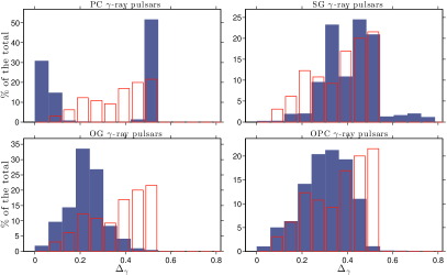
Figure 5 compares the $\gamma$-ray peak-separation distribution $\Delta_{\gamma}$ and the radio peak-separation distribution, $\Delta_{\mathrm{Radio}}$, for $\gamma$-ray-selected objects of all implemented models and LAT pulsars in the left and right panels, respectively. The observed $\Delta_{\gamma}$ distribution shown in figure 5 left panel, ranges in the interval 0.1$\hbox{\raise 2.15277pt\hbox{$<\lower 4.56386pt\hbox{$\kern-10.70009pt{\sim}$}$}}\Delta_{\gamma}\hbox{\raise 2.15277pt\hbox{$<\lower 4.56386pt\hbox{$\kern-10.70009pt{\sim}$}$}}$0.55 and shows two peaks at $\Delta_{\gamma}\sim$0.2 and $\Delta_{\gamma}\sim$0.5. None of the proposed emission geometries manages to explain the observations, but the SG and OPC models predict the observed distribution at high and low $\Delta_{\gamma}$ values, respectively; the 2KS test results listed in Table 4 shows that SG and OPC models explain the observations with the highest and second highest statistical significance, respectively. The PC model predicts $\Delta_{\gamma}$ just at low and high values: $\Delta_{\gamma}<$0.1 are generated by each magnetic pole hollow cone while $\Delta_{\gamma}\sim$0.5 are generated by the two emission cones from each magnetic pole separated by 0.5 in phases that start to be visible for high $\alpha$ and $\zeta$ (see Figure 15). The OG distribution is antithetic to the observed distribution. This distribution shows a maximum at $\Delta_{\gamma}\sim$0.2 which is consistent with the observations but goes to 0 at $\Delta_{\gamma}=$0.5 where the observed distribution shows its absolute maximum. The SG model explains the observations just for $\Delta_{\gamma}>$0.4, exhibits one peak at 0.35, which does not show up in the data, and clearly underestimates the observations for $\Delta_{\gamma}<$0.25. The OPC $\Delta_{\gamma}$ distribution shows a good consistency with observations for $\Delta_{\gamma}<$0.25 but completely fails to explain the observations at high $\Delta_{\gamma}$. We note that SG and OPC are complementary in how they explain the observed $\Delta_{\gamma}$ distribution and how the different prescription for the gap width computation in the OPC model affects the peak-separation distribution. The OPC prescription for the gap width allows for wider light-curve double peaks since the gap widths are generally smaller than those of the OPC and this is evident by comparing the OG and OPC peak-separation distributions; the OG distribution peaks at 0.2 and quickly goes to zero at $\Delta_{\gamma}$=0.5, while the OPC distribution shows a broad peak in the interval 0.2 $<\Delta_{\gamma}<$ 0.4 and slowly decrease to a non-zero minimum at $\Delta_{\gamma}$=0.5. This partially solves the complete lack of $\Delta_{\gamma}$=0.5 in the OG model and allows the OPC to explain, even poorly, the observed trend. However the vast majority of observed $\Delta_{\gamma}$=0.5 objects suggests that a SG-like two-pole caustic emission geometry is necessary to explain the wide separation of the observed $\gamma$-ray peaks, which, on the other hand, does not explain objects with $\Delta_{\gamma}<$ 0.25.

The $\gamma$-ray peak-separation distribution was also studied in the framework of PSRCAT2. Those authors performed a $\gamma$-ray light-curve analysis with the purpose to give the most precise possible measures of the peak positions and separations. Even though the purpose of our light-curve analysis is not to give precise measurements of peak positions and separations but to measure observed and simulated light curves under the same criteria to be compared, our $\Delta_{\gamma}$ distribution for LAT ordinary pulsars is consistent with the distribution obtained by PSRCAT2.

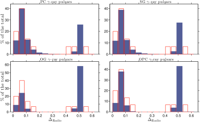
The observed radio peak-separation distribution shown in the right panel of Figure 5 ranges in two intervals, 0$<\Delta_{\mathrm{Radio}}<$0.15, where it peaks at $\Delta_{\mathrm{Radio}}\sim$0.05, and 0.4$\hbox{\raise 2.15277pt\hbox{$<\lower 4.56386pt\hbox{$\kern-10.70009pt{\sim}$}$}}\Delta_{\mathrm{Radio}}\hbox{\raise 2.15277pt\hbox{$<\lower 4.56386pt\hbox{$\kern-10.70009pt{\sim}$}$}}$0.55. A comparison of the $\Delta_{\mathrm{Radio}}$ observed and simulated distribution in the framework of each model shows that all of the proposed emission geometries explain the observed trend for low peak separation $\Delta_{\mathrm{Radio}}<$0.15 while for $\Delta_{\mathrm{Radio}}>$0.4 all models over predict the observations. This may be due to a radio cone used in our simulation that is too large and that increases the probability that the line of sight intersects the emission from both poles. The 2KS tests shown in Table 4 suggest that all models explain well the observations with the two-pole emission geometries, PC and SG, best explaining the LAT distribution since they predict the observed proportion. In analogy to the PC geometry, the $\Delta_{\mathrm{Radio}}\sim$0.1 are generated by double-peak structures typical of each radio emission beam, while $\Delta_{\mathrm{Radio}}\sim$0.5 are given by the distances of the two emission cones from each magnetic pole for high $\alpha$ and $\zeta$ (see Figure 15).

4.2 Radio lag

We consider the radio and $\gamma$-ray light curves of the same pulsar, both coherent in phase with the actual pulsar rotational phase. The radio lag is then defined as the phase lag between a radio fiducial phase and the following $\gamma$-ray peak phase. The radio lag is considered as a tracker of the pulsar magnetosphere structure. The radio lag constrains the relative positions of $\gamma$-ray and radio emission regions in the pulsar magnetosphere and can be used to discriminate the proposed $\gamma$-ray and radio emission geometries that best explain the observations. While it is relatively easy to produce radio and $\gamma$-ray light curves that are both coherent in phase with the pulsar rotation through timing techniques, the definition of the radio fiducial phase is more controversial. The commonly accepted definition for the radio fiducial phase is the phase of the radio peak following the pulsar magnetic pole that should be identified, case by case, by analysing the light-curve shape. However, this definition is strongly dependent on the light-curves quality, which might not be good enough to enable a robust identification of the magnetic pole, and might be biased by the radio model used to predict the magnetic pole phase in the observed light curve.

In PSRCAT2 the problem of finding solid criteria to assign a radio fiducial phase to observed light curves was solved by increasing the quality of the radio light curve with deeper radio observations of the analysed objects and by defining a series of morphological criteria. When the light curve shows symmetric structures (double or higher multiplicity peaks) the pulsar fiducial phase is associated with the peak barycentre. When radio and $\gamma$-ray peaks are aligned (e.g. Crab pulsar), the radio emission cannot be explained by a conical beam generated above the magnetic poles but rather by caustic emission, as proposed for the Crab pulsar by Venter et al. (2012). In these cases the fiducial phase is associated with the phase of the radio precursor, which is a small light-curve feature

The problem of finding a robust definition for the radio fiducial phase becomes critical when one compares simulations with observations. The magnetic-pole phase for simulated objects is known with high precision, it is independent of the assumed radio and $\gamma$-ray emission geometries, and is not affected by the light-curve quality. It is thus easy to identify the phase of the first peak after the magnetic pole. Moreover, the cone plus core radio emission geometry we adopt does not predict caustic radio emission and no aligned radio and $\gamma$-ray peaks are possible. The obvious consequence is that observed and simulated radio-lag measurements are not completely consistent and the conclusions drawn from their comparison loses scientific reliability. The radio lag for simulated objects has been computed as the phase separation between the first radio peak detected by the analysis algorithm, the fiducial phase, and the phase of the following $\gamma$-ray peak. Both $\gamma$-ray and radio simulated light curves have been generated within the phase interval -0.5 to 0.5 with the pulsar fiducial plane (the plane containing magnetic and rotational axes) intersecting the line of sight at phases 0 and $\pm$0.5. Because of that, the fiducial phase was prevalently found at phase 0 and, for large $\alpha$ and $\zeta$ values, at phase -0.5 (see Figure 15). In two-pole $\gamma$-ray emission geometries, PC and SG, each magnetic pole shines both in radio and in $\gamma$-rays, and the radio lag is always measured between the fiducial phase and the $\gamma$-ray beam coming from the same magnetic hemisphere. In one-pole $\gamma$-ray emission geometries there is just one magnetic hemisphere that shines in $\gamma$-rays and when, for large $\alpha$ and $\zeta$, radio emission from both magnetic poles starts to be visible in the light curve, cases of radio lag larger than 0.5 are possible; e.g. when radio emission beam starts shining at phase -0.5, the algorithm sets the fiducial phase equal to -0.5 and measures the radio lag as its distance from the $\gamma$-ray peak generated in the opposite magnetic hemisphere. All $\delta>$0.5 for OG and OPC models were subtracted of 0.5 to measure the radio lag as the phase lag between fiducial phase and $\gamma$-ray peak in the framework of the same magnetic hemisphere.

Figure 6: Radio-lag distribution for simulated samples (grey) and LAT pulsars (red) and each model.

We use the radio and $\gamma$-ray light curves published in PSRCAT2 to estimate the radio lags of RL LAT pulsars as the phase separation between the fiducial phase and the following $\gamma$-ray peak. We define the fiducial phase as the phase of the first peak, which appears in the radio light curve as detected from the algorithm described in Sections 3 and 4, to measure the radio lag for RL LAT pulsars consistent with the simulated sample. When two peaks separated by 0.5 in phase are visible in the radio light curve, we assign the fiducial phase to the radio peak for which the radio lag is smaller than 0.5. In this way we avoid the assumption about the magnetic pole position and the radio precursor that is not modelled in the framework of the implemented radio-beam emission geometry.

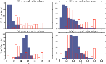
Figure 6 compares the radio lag $\delta$ distribution of simulated and observed RL pulsars in the framework of each model. A comparison between our $\delta$ distribution and the distribution obtained by PSRCAT2 shows a total consistency both in the range of values and in the proportions. Our $\delta$ distribution ranges in the interval $0<\delta<0.5$, and raises steeply up to its maximum at $\delta=0.15$ and shows a stable flat trend in the interval $0.2<\delta<0.5$. None of the tested models manages to explain the observed distributions over all the range of observed $\delta$ but the OPC shows higher agreement with the data. The 2KS test statistics given in Table 4 shows that the OPC model explains the observations with a CL at least four orders of magnitude larger than the other models and that the OG predictions explain the observations with the second highest CL. Both PC and SG models predict emission beams most of the time overlapping the radio emission beam, with the PC emission beam tightly matching the radio beam both in size and pulse phase (see Figure 15). This generates the excess of $\delta<$0.1 predicted by both PC and SG emission geometry with the SG geometry predicting larger $\delta$ values because of its wider emission beam. The OG model completely fails in predicting the observed distribution both in shape and proportions. The OPC is the model that best predicts the observed $\delta$ range and proportions. This model predicts a peak that is too broad in the range $0.15<\delta<0.25$ which partly overlap the observed peak but underestimates objects in the range $0.35<\delta<0.5$. Of particular interest is the difference between OG and OPC distributions. As also shown in Figure 5, the different prescription for the gap width adopted by the OPC enables broader light-curve peaks that occur closer, in phase, to the radio peak, thereby decreasing the radio lag. Under the assumption that the radio model used in this simulation is correct and that the adopted VRD magnetic field geometry is correct, this picture supports an outer magnetosphere location of the emission gap, points to the need to model broader light-curve $\gamma$-ray peaks, and highlights the importance of the gap width and B field structure choice in the light-curve modelling.

Figure 7: Distributions of the $\gamma$-ray and radio peak separation of simulated (grey) and observed (red) pulsars obtained, for each model, as a function of the $\gamma$-ray beaming factor are shown in the top and bottom panels, respectively. The model distributions have been obtained as two-dimensional number-density histograms. The dash-dotted line highlights the minimum number density contour. The LAT measurements are given with 1$\sigma$ error bar uncertainty.

One has to note that the model radio lags obtained in this study are strongly dependent on the assumed VRD magnetic field geometry. Kalapotharakos et al. (2012) compute the $\gamma$-ray light curves in a dissipative magnetosphere (DM) with conductivity ranging from 0 to $\infty$, corresponding to VRD magnetic field geometry and to a force-free electrodynamics (FFE) magnetic field geometry, respectively. Those authors conclude that VRD magnetospheres shows the smallest radio to $\gamma$-ray lags while more realistic DMs predict average larger lags (Kalapotharakos et al., 2012). All $\gamma$-ray model radio-lag distributions computed in this study would be shifted towards higher values if computed in the framework of a DM, and this would solve the excess of low radio-lag values predicted by the PC and SG models. Particularly interesting is the case of the SG model that shows the correct shape of the observed radio-lag distribution but shifted towards values that are too low; the implementation of the SG model within a DM may considerably improve the SG prediction.

4.3 Non-observable pulsar parameters: $\Delta_{\gamma}$, $\Delta_{\mathrm{Radio}}$, and $\delta$ as a function of f_Ω, $\alpha$, $\zeta$

We compare simulated and estimated correlations between $\Delta_{\gamma}$, $\Delta_{\mathrm{Radio}}$, and $\delta$ and non-observable pulsar parameters, namely beaming factor $f_{\Omega}$, magnetic obliquity $\alpha$, and observer line-of-sight $\zeta$. The simulated distributions of $f_{\Omega}$, $\alpha$, and $\zeta$ are those synthesised in the framework of PC, SG, OG, and OPC emission models by PIERBA12 via the emission geometry proposed by Dyks et al. (2004). The same parameters for LAT pulsars have been estimated from fits to the observed pulsar light curves by PIERBA15 in the framework of the same emission models and using the same emission geometry by Dyks et al. (2004).

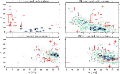
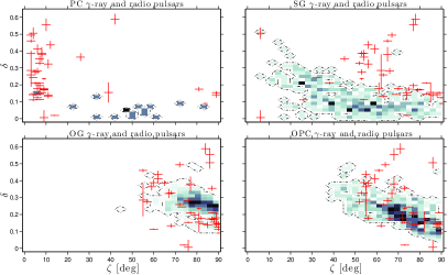
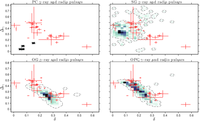
The simulation by PIERBA12 gives the allowed range of values for the parameters $f_{\Omega}$, $\alpha$, and $\zeta$ within each model. Since $f_{\Omega}$, $\alpha$, and $\zeta$ for LAT pulsars were estimated by implementing the same geometrical model used by PIERBA12 to synthesise the simulated-population light curves, we expect a match between estimations and simulations within the same model only if the model manages to reproduce the variety of the observed light-curve shapes. If the variety of observed light-curve shapes is not explained in the framework of a particular model, the best-fit parameters $f_{\Omega}$, $\alpha$, and $\zeta$ does not match the interval of the most likely values as simulated by PIERBA12 in the framework of the same model. Because of that, a mismatch between estimated (PIERBA15) and simulated (PIERBA12) trends in the framework of a particular model suggests the inadequacy of that model in explaining the observations. An example of inadequacy of a model in explaining the observed light curves is given by the PC model and it is evident by looking at the PC panel at the top of Figure 8. The vast majority of the PC light curves show sharp peaks and low off-peak emission that do not manage to predict the variety of the LAT light-curve shapes. This implies that the PIERBA15 fitting algorithm selects as best-fit solutions only PC light curves with very low $\alpha$ and $\zeta$ angles, which are those characterised by broader peaks and more likely to explain the observed shapes (see Figure 15). As a consequence, in the PC panel of Figures 8 and 9, the estimated points are all grouped at low $\alpha$ and $\zeta$ values and do not match the $\alpha$ and $\zeta$ intervals predicted by the PC simulation. This suggests the inadequacy of the PC model in predicting the observations. The statistical agreement between observed/estimated and simulated distributions was quantified by computing the two-sample Kolmogorov-Smirnov (2KS) statistics for the two-dimensional distributions proposed by Press et al. (1992) as described in Section E. The D and $p_{\mathrm{value}}$ values computed between each observed/estimated and simulated distribution are listed in Table 5.

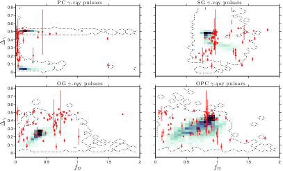
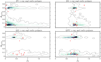
Figure 7 compares estimated and simulated distributions for $\Delta_{\gamma}$ and $\Delta_{\mathrm{Radio}}$ as a function of the beaming factor $f_{\Omega}$ and for each model. The $\Delta_{\gamma}$-$f_{\Omega}$ plane is a tracker of the magnetospheric region where the $\gamma$-ray emission is generated since both $\Delta_{\gamma}$ and $f_{\Omega}$ depends on the emission-region structure. Overall none of the distributions estimated in the framework of the proposed emission geometries matches the simulated ranges but the SG and OG models show consistency with observations at the highest and second highest CL, respectively, as indicated in Table 5. Both OG and OPC models show highly dispersed distribution and suggest that, for the bulk of the simulated distributions, $\Delta_{\gamma}$ increases as $f_{\Omega}$ increases. The OPC estimates match the simulations only for $f_{\Omega}>$0.4 since they manage to reproduce the bulk of objects centred at $f_{\Omega}\sim$0.85 and $\Delta_{\gamma}\sim$0.45 while the OG estimates do not match the bulk of the simulated objects. The PC and SG models do not predict any $\Delta_{\gamma}$ variation as $f_{\Omega}$ changes and, in both cases, the estimates do not match the bulk of the simulations. In the $\Delta_{\mathrm{Radio}}$-$f_{\Omega}$ plane, all model estimates reasonably match the simulated trends and given the low number of observed objects, the relative $p_{\mathrm{values}}$ listed in Table 5 cannot be used to discriminate the model that best explains the data.

Figure 8: Distributions of the $\gamma$-ray and radio peak separation of simulated (grey) and observed (red) pulsars obtained, for each model, as a function of the magnetic obliquity are shown in the top and bottom panels, respectively. The model distributions have been obtained as two-dimensional number-density histograms. The dash-dotted line highlights the minimum number density contour. The LAT measurements are given with 1$\sigma$ error bar uncertainty.

Figure 9: Distributions of the $\gamma$-ray and radio peak separation of simulated (grey) and observed (red) pulsars obtained, for each model, as a function of the observer line of sight are shown in the top and bottom panels, respectively. The model distributions have been obtained as two-dimensional number-density histograms. The dash-dotted line highlights the minimum number density contour. The LAT measurements are given with 1$\sigma$ error bar uncertainty.

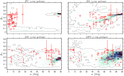
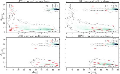
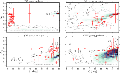
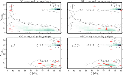
Figures 8 and 9 compare estimated and simulated trends of $\Delta_{\gamma}$ and $\Delta_{\mathrm{Radio}}$ as function of $\alpha$ and $\zeta$, respectively. The parameters $\Delta_{\gamma}$ and $\Delta_{\mathrm{Radio}}$ are expected to change with increasing $\alpha$ and $\zeta$ with different trends and in the framework of different emission geometries, as shown in Figure 15. In the PC and radio emission geometries, the size of the conical emission beams decrease as $\alpha$ and $\zeta$ increase, therefore $\Delta_{\gamma}$ and $\Delta_{\mathrm{Radio}}$ are expected to decrease with increasing $\alpha$ and $\zeta$. This behaviour is barely visible in the PC $\gamma$-ray separation but it is evident in the radio cases for PC and SG-selected objects. The PC estimates populate the low $\alpha$ and $\zeta$ regions of the $\Delta_{\gamma/radio}$-$\alpha$ and $\Delta_{\gamma/radio}$-$\zeta$ planes, respectively, and do not match the major fraction of simulated points. The SG model predicts increasing $\Delta_{\gamma}$ when both $\alpha$ and $\zeta$ increase. As shown in figure 15, the bright SG caustic widens when $\zeta$ increases for fixed $\alpha$ and when $\alpha$ increases, the caustic from the second magnetic pole starts to be visible in the light curve and $\Delta_{\gamma}$ tend to 0.5. In both $\Delta_{\gamma}$-$\alpha$ and $\Delta_{\gamma}$-$\zeta$ planes, the SG estimates match the simulated trends. The OG and OPC models are explained in the framework of a one-pole caustic emission geometry; when $\alpha$ increases, no emission from the other pole shows up at high $\zeta$ and $\Delta_{\gamma}$ does not tend to 0.5 as $\alpha$ or $\zeta$ increase. This is less evident in the OPC model predictions where, because of the different prescription for the gap width, wider peaks are possible and both $\Delta_{\gamma}$-$\alpha$ and $\Delta_{\gamma}$-$\zeta$ trends show broader distributions. Both figures 8 and 9 show that $\Delta_{\gamma}$ increases for increasing $\alpha$ or $\zeta$ with the OPC trend showing higher dispersion with respect to the OG trend as a result of the different prescription used in the OPC to compute the width of the accelerator gap. In the plane $\Delta_{\gamma}$-$\alpha$, neither OG nor OPC estimates match the bulk of the simulated distribution; in both cases, the estimates show an excess at $\Delta_{\gamma}=0.5$, which is not predicted by the models. In the plane $\Delta_{\gamma}$-$\zeta$, the OG estimates over predict $\Delta_{\gamma}=0.5$ and fail again in matching the bulk of the simulated distribution, while the OPC estimates match the simulation explaining the simulated increasing trend well. The results of the statistical test shown in Table 5 find that in the plane $\Delta_{\gamma}$-$\alpha$, PC and SG models predict the observations with the highest and second highest CL while in the $\Delta_{\gamma}$-$\zeta$ plane, the OG and SG models give the highest and second highest CL predictions of the data. The best agreement obtained between observed/estimated and simulated distributions in the plane $\Delta_{\gamma}$-$\alpha$ is fictitious since the distributions are totally not overlapping and inconsistent.

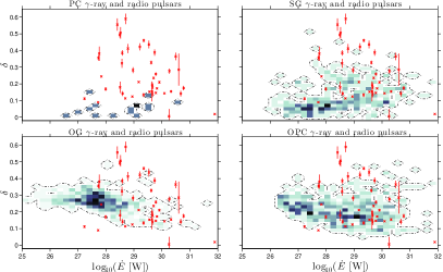
In the $\Delta_{\mathrm{Radio}}$-$\alpha$ and $\Delta_{\mathrm{Radio}}$-$\zeta$ planes, as a consequence of the radio beam shrinking with increasing $\alpha$ or $\zeta$, the simulated $\Delta_{\mathrm{Radio}}$ are expected to decrease with increasing $\alpha$ and $\zeta$, especially at low angles, as is evident from Figure 15. This trend is well visible in the PC- and SG-selected objects with $\alpha$ and $\zeta$ values ranging from 0 to 90 degree while the trend is not appreciable for OG- and OPC-selected objects, which are mainly characterised by high $\alpha$ and $\zeta$. Radio objects selected in the framework of all $\gamma$-ray models show an excess for $\alpha$ and $\zeta$ $>70^{\circ}$ and $\Delta_{\gamma}$=0.5. As in the PC case, this excess is a consequence of the radio emission from the other pole that, for high $\zeta$ angles, starts to be visible for high $\alpha$ values and allows peak separations equal to the magnetic pole distance, 0.5. Overall, all model estimates match the simulated trends with consistent CL with PC and OG showing the highest CL in the $\Delta_{\mathrm{Radio}}$-$\alpha$ and $\Delta_{\mathrm{Radio}}$-$\zeta$ planes, respectively (see Table 5).

Figure 10 compares estimated and simulated trends for $\delta$ as functions of $f_{\Omega}$, $\alpha$, and $\zeta$, in the top, middle, and bottom panels, respectively. In the $f_{\Omega}$-$\delta$ plane, the two-pole emission geometries PC and SG, do not predict any trend for $\delta$ changing with increasing $f_{\Omega}$ while the one-pole caustic models, OG and OPC, predict mild decreasing $\delta$ as $f_{\Omega}$ increases. The estimates obtained in the framework of PC and SG emission geometries fail to match the model prediction and do not match the bulk of the objects modelled while OG and OPC estimates match the bulk of the model prediction and seem to best represent the modelled behaviour showing, the highest and second highest $p_{\mathrm{value}}$ (see Table 5).

Figure 10: Distributions of the radio lag of simulated (grey) and observed (red) pulsars obtained, for each model, as a function of the $\gamma$-ray beaming factor, magnetic obliquity, and observer line of sight are shown in the top, central, and bottom panels, respectively. The model distributions have been obtained as two-dimensional number-density histograms. The dash-dotted line highlights the minimum number density contour. The LAT measurements are given with 1$\sigma$ error bar uncertainty.

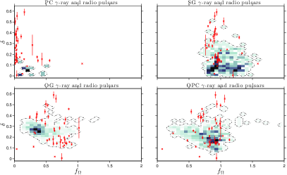
In the $\alpha$-$\delta$ and $\zeta$-$\delta$ planes, a decreasing trend of $\delta$ as $\alpha$ and $\zeta$ increase clearly shows up in the simulations for all models except for the PC. This behaviour can be explained in the light of figure 15; as $\alpha$ increases, the bright caustic approaches the radio emission beam, thereby decreasing $\delta$. The very same behaviour is observed in each phase-plot panel when $\zeta$ increases for fixed $\alpha$ values; in both SG and OG/OPC emission geometry the bright caustic gets closer to the radio emission beam when $\zeta$ increases. The same decreasing trend should also be observed in the PC model prediction since $\gamma$-ray and radio emission beams get closer when $\alpha$ increase but the trend does not show up because of the paucity of simulated PC objects. The outer and intermediate-high magnetosphere model estimates from OPC and SG best match the modelled trends showing the largest $p_{\mathrm{value}}$ values (see Table 5.)

Figure 11: Distributions of the $\gamma$-ray peak separation, radio peak separation, and radio lag of simulated (grey) and observed (red) pulsars obtained, for each model, as a function of the spin-down power are shown in the top, central, and bottom panels, respectively. The model distributions have been obtained as two-dimensional number-density histograms. The dash-dotted line highlights the minimum number density contour. The LAT measurements are given with 1$\sigma$ error bar uncertainty.

4.4 Observable pulsar parameters: $\Delta_{\gamma}$, $\Delta_{\mathrm{Radio}}$, and $\delta$ as a function of spin-down power $\dot{E}$ and spin period P

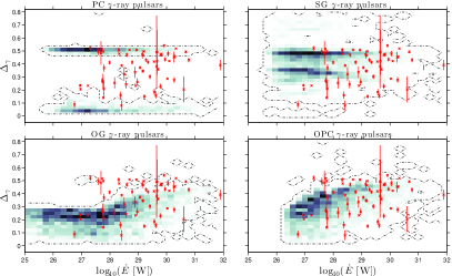
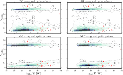
We compare the simulated and observed correlations between $\Delta_{\gamma}$, $\Delta_{\mathrm{Radio}}$, and $\delta$ and pulsar spin-down power $\dot{E}$ and spin period P. Simulated and observed $\dot{E}$ values were computed as described in PIERBA12 while the LAT pulsar spin periods have been taken from PSRCAT2. The statistical agreements between observed and simulated distributions are given in Table 5. Figure 11 compares observed and simulated trends of $\Delta_{\gamma}$, $\Delta_{\mathrm{Radio}}$, and $\delta$ as a function of $\dot{E}$ in the top, middle, and bottom panels, respectively. The comparisons of simulated and observed trends in the framework of all models reflect the same inconsistency shown in PIERBA12; none of the simulated emission geometries manage to explain the behaviour of the observed sample at high $\dot{E}$ showing a deficiency of high-$\dot{E}$ objects with respect to the observations.

Figure 12: Distributions of the $\gamma$-ray peak separation, radio peak separation, and radio lag of simulated (grey) and observed (red) pulsars obtained, for each model, as a function of the spin period are shown in the top, central, and bottom panels, respectively. The model distributions have been obtained as two-dimensional number-density histograms. The dash-dotted line highlights the minimum number density contour. The LAT measurements are given with 1$\sigma$ error bar uncertainty.

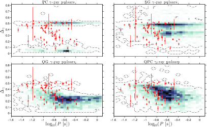
In the plane $\Delta_{\gamma}$-$\dot{E}$ the PC model completely fails to explain the observations. As already shown in Figure 5, the SG model predicts a double $\Delta_{\gamma}$ distribution. The first distribution is centred at $\Delta_{\gamma}$=0.5 and is given by the separation of the peaks coming from each magnetic pole caustic at high $\alpha$ and does not change with increasing $\dot{E}$. The second distribution is centred at $\Delta_{\gamma}$=0.35, is given by the separation of the double peaks generated by the same magnetic-pole caustic, and shows a mild decrease with increasing $\dot{E}$ due to the shrinking of the SG beam as $\dot{E}$ increases. The models SG and OPC best explain the observations with OPC best predicting the observed behaviour. The OG model over predicts low $\dot{E}$ objects for $\dot{E}<10^{26.5}$W, while OPC does not predict any object in the same interval. The $p_{\mathrm{value}}$ values listed in Table 5 shows that in most of the cases, OPC and OG describe the observed distributions at the higher CL with the SG predictions best explaining the observations on plane $\dot{E}$-$\Delta_{\gamma}$.

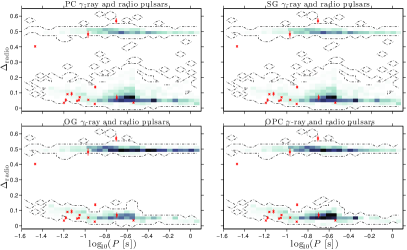
The $\dot{E}$-$\Delta_{\gamma}$ correlation was also studied in the framework of PSRCAT2. A comparison of the LAT pulsars $\dot{E}$-$\Delta_{\gamma}$ correlation obtained here and in the framework of PSRCAT2 shows consistency between the two $\Delta_{\gamma}$ computation techniques. As a result of more accurate $\Delta_{\gamma}$ measures, the $\dot{E}$-$\Delta_{\gamma}$ correlation obtained by PSRCAT2 shows clearer evidence of a double trend that is similar to our SG model predictions but centred at lower $\Delta_{\gamma}$ values of 0.43 and 0.22, with no apparent decrease of the $\Delta_{\gamma}$ as $\dot{E}$ increase. In the $\dot{E}$-$\Delta_{\mathrm{Radio}}$ plane all $\gamma$-ray-selected radio pulsars show the same double trend at constant $\dot{E}$ values, 0.05 and 0.5, with the OPC-selected radio sample preferred to explain the observations. In the $\dot{E}$-$\delta$ plane, all implemented emission geometries fail to explain how the radio lag changes with increasing $\dot{E}$. Both PC and SG models do not show any trend in $\delta$ changing with increasing $\dot{E}$, while the one-pole caustic models, OG and OPC, show a mild trend in $\delta$ decreasing with increasing $\dot{E}$.

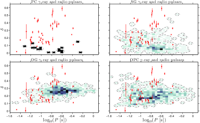
Figure 12 compares observed and simulated trends of $\Delta_{\gamma}$, $\Delta_{\mathrm{Radio}}$, and $\delta$ as a function of spin period P in the top, middle, and bottom panels, respectively. In contrast tom the $\dot{E}$ computation, which requires assumptions on the pulsar mass, radius, and moment of inertia, the spin period is na assumption-independent of observed characteristics. An increase of P implies an increase of the light-cylinder radius corresponding to a decrease of the open magnetic field-line region. In the P-$\Delta_{\gamma}$ plane, the observed sample shows a two-component distribution: one with objects characterised by $\Delta_{\gamma}\sim$0.5 as $P$ increases and one showing $\Delta_{\gamma}$ decreasing as P increases for $\Delta_{\gamma}\hbox{\raise 2.15277pt\hbox{$<\lower 4.56386pt\hbox{$\kern-10.70009pt{\sim}$}$}}$0.45. Both OG and OPC predict the observed decreasing component as P increases but overestimate the high P objects and fail to explain the observed flat component at $\Delta_{\gamma}\sim$0.5. The OPC best explains the observations since best describes the observed distribution over the entire $P$ interval. In the PC case, the model predictions completely fail to explain the observed decreasing trend. The increase of the light-cylinder radius implies a shrinking of the conical emission beams and a decrease of $\Delta_{\gamma}$ with P.

Figure 13: Distributions of the $\gamma$-ray and radio peak separation of simulated (grey) and observed (red) pulsars obtained, for each model, as a function of radio lag are shown in the left and right panels, respectively. The model distributions have been obtained as two-dimensional number-density histograms. The dash-dotted line highlights the minimum number density contour. The LAT measurements are given with 1$\sigma$ error bar uncertainty.

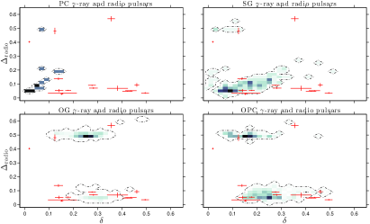
Because of the paucity of PC simulated objects, a mild peak separation decrease is observed just for the $\gamma$-ray-selected radio simulated objects and for P$<$125ms. The SG model predicts a constant double distribution centred at $\Delta_{\gamma}$ values of 0.35 and 0.5. The model explains the constant $\Delta_{\gamma}\sim 0.5$ branch but fails to describe the observed decreasing trend. The fact that PS/SG and OG/OPC best predict the flat and decreasing component of the observed distribution, respectively, is because of the two-pole and one-pole nature of their emission, respectively; the two-pole emission predicts more 0.5 separated peaks from both the poles, while in one-pole emission, 0.5 separated peaks only occur in the shorter P light curves. In the P-$\Delta_{\mathrm{Radio}}$ plane the radio objects selected in framework of each $\gamma$-ray model give the very same explanation of the observed points and cannot be used to discriminate the model that best explains the observations.

In the plane P-$\delta$ none of the emission geometries manages to describe the observed trend but the OPC models seem to give a better description of the observations. The shrinking of the open field-line region as a consequence of the increase of P implies a simultaneous shrinking of both radio and $\gamma$-ray beams in the framework of each model. In the SG case (and mildly in the PC), we observe a decreasing trend in $\delta$ as P increases, which could be explained by a faster shrinking of the radio emission beam with respect to the PC beam and as a consequence of the SG caustic approaching the radio beam as P increases, respectively. The OG and OPC model predictions are not able to explain the observations; both OG and OPC simulations are characterised by a mild increase of $\delta$ as P increases, which is not present in the observed distribution. The statistical significance with which the modelled distributions for $\Delta_{\gamma}$, $\Delta_{\mathrm{Radio}}$, and $\delta$ as a function of $P$ explain the observations partly mimic that obtained for the same parameters as a function of $\dot{E}$. The OPC model explains the observed distributions at the higher CL in the planes $\Delta_{\gamma}$-P and $\delta$-P, while the PC model predictions best explain the observations on the plane $P$-$\Delta_{\mathrm{Radio}}$.

4.5 $\gamma$-ray and radio peak separation as a function of the radio lag

The relation $\Delta_{\gamma}$ vs. $\delta$ is particularly important in the study of the pulsar emission geometry and magnetosphere structure since it correlates with information on the magnetospheric regions where $\gamma$-ray and radio emission are generated: $\Delta_{\gamma}$ is a function of the pulsar gap width structure while $\delta$ constrains the relative position of $\gamma$-ray and radio emission regions. The $\Delta_{\gamma}$ vs. $\delta$ correlation was first studied by Romani and Yadigaroglu in 1995 . By analysing the light curves of six radio pulsars detected in $\gamma$-rays from the Compton gamma-ray observatory (CGRO), those authors concluded that $\Delta_{\gamma}$ shows a decreasing trend of increasing $\delta$. With the sizeable increase of the number of $\gamma$-ray and radio active pulsars because of the advent of the Fermi satellite, it was finally possible to give more precise estimates of the $\delta$-$\Delta_{\gamma}$relation. Watters et al. (2009) performed a first measurement of $\delta$ and $\Delta_{\gamma}$ for six RL LAT pulsars confirming the trend $\Delta_{\gamma}$ decreasing with increasing $\delta$. The trend was further confirmed in the framework of PSRCAT1 on a sample of 17 RL pulsars and by independent analyses on the same pulsar sample performed by Pierbattista (2010). The last and more accurate $\delta$ and $\Delta_{\gamma}$ measurements were obtained in the framework of PSRCAT2; these measurements concern 32 pulsars and confirm the previous findings of $\Delta_{\gamma}$ decreasing with increasing $\delta$. In all the above mentioned cases, the radio lag $\delta$ was computed as the distance between the fiducial phase computed according to PSRCAT2 criteria (estimated position of the magnetic pole) and the phase of the following$\gamma$-ray peak. Since radio and $\gamma$-ray peak refer to the same magnetic pole, no $\delta>0.5$ is allowed.

We compared simulated and observed correlations $\Delta_{\gamma}$ vs. $\delta$ and $\Delta_{\mathrm{Radio}}$ vs. $\delta$. For both simulated and observed objects, $\Delta_{\gamma}$ and $\Delta_{\mathrm{Radio}}$ have been computed as described in Section 4.1 while the computation technique of $\delta$ is described in Section 4.2. We studied how the radio peak separation changes with increasing $\delta$ to constrain the structure of the radio emission region against the models.

Figure 13 compares observed and simulated trends for $\Delta_{\gamma}$ vs. $\delta$ and $\Delta_{\mathrm{Radio}}$ vs. $\delta$ in the left and right panels, respectively. In the $\delta$-$\Delta_{\gamma}$ plane, the LAT objects follow a clearly decreasing trend of $\Delta_{\gamma}$ when $\delta$ increases. The PC model fails completely to explain the observations, predicting a distribution in total disagreement with the observations. Points are only predicted for small $\delta$ and $\Delta_{\gamma}$ values and seem to show a trend of increasing $\Delta_{\gamma}$ with increasing $\delta$. The same increasing trend and inconsistency with the observations was obtained by Pierbattista (2010) comparing simulations and PSRCAT1 observations . The SG model does not explain the observed decreasing trend, predicts observations mainly at low $\delta$ and intermediate $\Delta_{\gamma}$ and shows a mild increasing trend of $\Delta_{\gamma}$ with increasing $\delta$. Comparisons of SG simulations against observations were performed by Watters et al. (2009) and by Pierbattista (2010) on six $\gamma$-ray pulsars (see references in Watters et al. (2009)) and on the pulsars from PSRCAT1, respectively. The two studies found results consistent with each other and also conclude that the SG model does not explain the observed $\delta$-$\Delta_{\gamma}$ trend. The one-pole emission geometry manages to explain the LAT findings successfully. Both the OG and OPC models manage to reproduce the shape of the observed distribution with the OPC showing higher agreement with observations. The $p_{\mathrm{value}}$ shown in Table 5 shows that, not including the PC model that shows a statistics that is too low to be correctly compared with observations, the OPC and OG are the models that explain the observed $\Delta_{\gamma}$ as a function of $\delta$ with the highest and second highest CL, respectively. Comparisons of OG simulations against observations were also performed by Watters et al. (2009) and Pierbattista (2010) on six $\gamma$-ray pulsars and on the pulsars from PSRCAT1, respectively (see Watters et al. (2009) and PSRCAT1 for references about the LAT pulsars). In both studies, the OG model predicts a decreasing trend of $\Delta_{\gamma}$ as $\delta$ increases consistent with the current findings. It is proper to stress again (see Section 4.2) that the results obtained in this study are strongly dependent on the VRD magnetic field geometry assumed. The assumption of a more realistic DM geometry would imply larger radio to $\gamma$-ray lags predicted by all implemented $\gamma$-ray models (Kalapotharakos et al., 2012). This would shift all observed distributions towards higher $\delta$ and would probably imply an improvement of the SG model predictions in explaining the observations.

In the plane $\delta$-$\Delta_{\mathrm{Radio}}$ the LAT objects follow a clear flat trend with $\Delta_{\mathrm{Radio}}$ stable at 0.05 with increasing $\delta$. Both PC and SG models predict an increase of $\Delta_{\mathrm{Radio}}$ as $\delta$ increases, which is not observed in the LAT data. The simultaneous increase of $\Delta_{\gamma}$ and $\Delta_{\mathrm{Radio}}$ as $\delta$ increases could be explained by the radio emission beam size, which increases at a higher rate than the PC and SG beam sizes, thereby increasing the distance between the first radio peak and the first $\gamma$-ray peak. Both outer magnetosphere models, OG and OPC, correctly predict the observed behaviour with the OPC explaining the observed range of $\delta$ values. In the $\delta$-$\Delta_{\mathrm{Radio}}$ plane, the $p_{\mathrm{value}}$ shows that the OG and PC are the models that describe the observations with the highest and second highest CL, respectively.

5 The $\alpha$-$\zeta$ plane

Figure 14: From the first to the fourth row, the $\gamma$-ray light curve multiplicity (left column) and peak separation (right column) as a function of $\alpha$ and $\zeta$ for LAT pulsars and PC, SG, OG, and OPC models are shown respectively. Big triangles and small points refer to LAT and simulated pulsars, respectively.

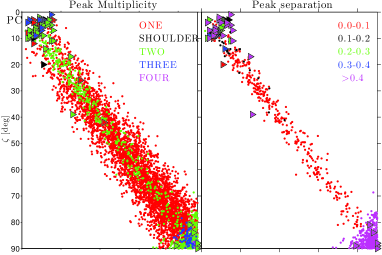
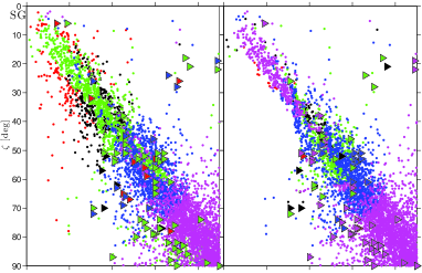
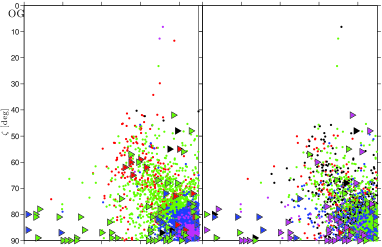
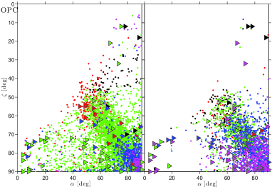
Figure 14 compares light-curve multiplicity and peak separation as a function of $\alpha$ and $\zeta$ for modelled and observed $\gamma$-ray light curves. The $\alpha$ and $\zeta$ of the LAT pulsars are taken from PIERBA15 while the $\alpha$ and $\zeta$ of the simulated objects are those synthesised by PIERBA12. Parameters $\alpha$ and $\zeta$ are non-observable pulsar characteristics and, analogous to what we previously discussed in Section 4.3, a match between LAT pulsar estimates and model prediction suggests that that model explains the observed variety of $\gamma$-ray pulsar light curves.

The plane $\alpha$ vs. $\zeta$ as a function of the peak multiplicity and peak separation and in the framework of PC, SG (two pole emission geometries), and OG (one pole emission geometry) was also studied by Watters et al. (2009). Our study shows that the geometrical characteristics as a function of the pulsar orientation of the light curves synthesised by PIERBA12 are consistent with the simulations by Watters et al. (2009). Moreover our analysis characterises the shoulder pulse shape that is recurrent among both synthesised and observed objects. Shoulder shapes are observed in the framework of the SG and OG/OPC geometries; in the SG model, the shoulder shape is associate with the $\alpha$-$\zeta$ plane region between single- and double-peak profiles, while in the OG/OPC geometry they do not represent the transition between single- and double-peak shapes but they are recurrent at high $\alpha$ and high $\zeta$. The best agreement between estimated parameters and the bulk of the model prediction is observed in the framework of the OPC model but there are inconsistencies in the peak separations plot (Figure 14), with the OG and OPC model predicting too few small $\alpha$ values than the fits to the LAT pulsars. The PC estimates completely fail to match the major part of the PC simulations for all $\alpha$ and $\zeta$. The SG estimates show inconsistencies in the light-curve peak multiplicity and pulsar orientation; many two peak pulsars are found at high $\alpha$ and low $\zeta$ where four peak profiles are found (see left side SG panel of Figure 14). The OG/OPC model estimates are consistent with model predictions for what concern both multiplicity and peak separation. Other plots showing $\alpha$ and $\zeta$ as a function of spin period (just for the PC)/gap width (SG, OG, and OPC) and light-curve peak multiplicity, are shown in Figures 19 and 20.

	PC		SG		OG		OPC
	$D$	$p_{\mathrm{value}}$ [%]	$D$	$p_{\mathrm{value}}$ [%]	$D$	$p_{\mathrm{value}}$ [%]	$D$	$p_{\mathrm{value}}$ [%]
Fig. 7
$\Delta_{\gamma}$ vs. $f_{\Omega}$	0.72	0.18	gray!600.40	gray!600.27	gray!300.55	gray!300.25	0.35	24
$\Delta_{\mathrm{radio}}$ vs. $f_{\Omega}$	gray!300.48	gray!300.18	0.29	0.16	gray!600.35	gray!600.26	0.29	0.17
Fig. 8
$\Delta_{\gamma}$ vs. $\alpha$	gray!600.69	gray!600.26	gray!300.23	gray!300.22	0.57	0.21	0.43	0.20
$\Delta_{\mathrm{radio}}$ vs. $\alpha$	gray!600.54	gray!600.23	gray!300.24	gray!300.20	0.39	0.19	0.39	0.16
Fig. 9
$\Delta_{\gamma}$ vs. $\zeta$	0.73	0.23	gray!300.23	gray!300.22	gray!600.45	gray!600.23	0.34	0.22
$\Delta_{\mathrm{radio}}$ vs. $\zeta$	0.51	0.14	0.24	0.15	gray!600.38	gray!600.22	gray!300.37	gray!300.18
Fig. 10
$\delta$ vs. $f_{\Omega}$	0.50	0.23	0.48	0.24	gray!600.32	gray!600.27	gray!300.34	gray!3025
$\delta$ vs. $\alpha$	0.52	0.24	gray!300.49	gray!300.25	0.38	0.24	gray!600.33	gray!600.28
$\delta$ vs. $\zeta$	0.51	0.22	gray!300.49	gray!300.24	0.32	0.21	gray!600.35	gray!600.27
Fig. 11
$\Delta_{\gamma}$ vs. $\dot{E}$	0.74	0.20	gray!600.53	gray!600.25	0.52	0.23	gray!300.49	gray!300.23
$\Delta_{\mathrm{radio}}$ vs. $\dot{E}$	gray!300.44	gray!300.23	0.40	0.20	0.43	0.19	gray!600.40	gray!600.29
$\delta$ vs. $\dot{E}$	0.56	0.24	gray!300.49	gray!300.26	gray!600.42	gray!600.28	0.39	0.24
Fig. 12
$\Delta_{\gamma}$ vs. $P$	0.71	0.22	gray!300.53	gray!300.24	0.47	0.23	gray!600.43	gray!600.27
$\Delta_{\mathrm{radio}}$ vs. $P$	gray!600.48	gray!600.23	gray!300.43	gray!300.19	0.49	0.16	0.45	0.17
$\delta$ vs. $P$	0.54	0.25	0.50	0.24	gray!300.39	gray!300.25	gray!600.38	gray!600.25
Fig. 13
$\Delta_{\gamma}$ vs. $\delta$	gray!300.43	gray!300.25	0.38	0.23	0.28	0.24	gray!600.25	gray!600.25
$\Delta_{\mathrm{radio}}$ vs. $\delta$	gray!300.16	gray!300.32	0.13	0.23	gray!600.12	gray!600.41	0.08	0.21

Table 5: Estimates of the consistency between observed/estimated and simulated two-dimensional distributions shown in Figures 7 to 13. The 2D-2KS statistics $D$ ranges between 0 and 1 for distributions showing total agreement and total disagreement, respectively. The $p_{\mathrm{value}}$ is the probability to obtain the observed $D$ value under the assumption that the two distributions are obtained from the same distribution (null hypothesis). This is equivalent to rejecting the null hypothesis at a confidence level of 100-($p_{\mathrm{value}}$)%. The 2D-2KS statistics and distributions are described in Section E. The $D$ and $p_{\mathrm{value}}$ parameters relative to the first and second most consistent distributions are highlighted in dark grey cells and light grey cells, respectively.

6 Summary

We compared the morphological characteristics of observed $\gamma$-ray and radio light curves with the same characteristics computed on a synthesised pulsar light-curve population in the framework of different $\gamma$-ray and radio geometrical models. The observed $\gamma$-ray and radio light curves are the young or middle-aged ordinary pulsars published in Abdo et al. (2013), while the simulated pulsar light curves are those synthesised by Pierbattista et al. (2012) assuming the magnetospheric emission geometry from Dyks et al. (2004) and in the framework of four $\gamma$-ray models and a radio model: Polar Cap (PC; Muslimov & Harding, 2003), Slot Gap (SG; Muslimov & Harding, 2004), Outer Gap (OG; Cheng et al., 2000), One Pole Caustic (OPC; Watters et al., 2009; Romani & Watters, 2010), and radio core plus cone models (Gonthier et al., 2004; Story et al., 2007; Harding et al., 2007).

For observed and simulated light curves and for each model we defined a series of morphological characteristics, namely peak number, light-curve minima, width of the peaks, among others, and built a $\gamma$-ray and radio shape classification according to the recurrence of these characteristics in the light curve. We evaluated the precise peak phases by fitting the light curve with a number of Gaussian and/or Lorentzian functions equal to light-curve peak number and computed $\gamma$-ray and radio peak separation distributions ($\Delta_{\gamma}$ and $\Delta_{\mathrm{Radio}}$, respectively) and the radio loud pulsars, radio-radio lag distribution ($\delta$) for observed objects and for the objects simulated in the framework of each model.

We studied how $\Delta_{\gamma}$, $\Delta_{\mathrm{Radio}}$, and $\delta$ changes as a function of observable pulsar characteristics, namely spin period (P) and spin-down power ($\dot{E}$), and as a function of non-observable pulsar characteristics like magnetic obliquity ($\alpha$), observer line of sight ($\zeta$), and $\gamma$-ray beaming factor ($f_{\Omega}$). The observable pulsar parameters are taken from the second catalogue of $\gamma$-ray LAT pulsars, (Abdo et al., 2013) while the non-observable LAT pulsar parameters were estimated in the framework of PC, SG, OG, and OPC models by Pierbattista et al. (2015). We compared the observed distributions of $\Delta_{\gamma}$, $\Delta_{\mathrm{Radio}}$, and $\delta$ with the same distributions obtained in the framework of the implemented $\gamma$-ray emission geometries. We also compared observed and simulated trends for $\Delta_{\gamma}$, $\Delta_{\mathrm{Radio}}$, and $\delta$ as a function of the observable parameters P and $\dot{E}$, and as a function of the non-observable/estimated pulsar parameters $\alpha$, $\zeta$, and $f_{\Omega}$. The comparison of the $\Delta_{\mathrm{Radio}}$ distribution and trends within each $\gamma$-ray models is possible because the RL pulsar population changes as a function of the different $\gamma$-ray visibility of each model and shows how the characteristics of a unique radio population change in the framework of its $\gamma$ ray-selected subsamples.

We studied how the recurrence of the shape classes changes between the whole simulated sample and its visible subsample and we obtained that no selection effects due to the light-curve shapes affect the pulsar visibility. This allowed us to compare the observed morphological characteristics with the same characteristics obtained on the whole simulated sample and within each model without applying the LAT $\gamma$-ray pulsar visibility to the simulated pulsar sample.

The agreement between the observed and simulated one-dimensional distribution in the framework of each model has been quantified by computing the 2KS test. Each 2KS statistics $D$, has been computed jointly with its $p_{value}$ expressing the probability of obtaining the $D$ value assuming that the two one-dimensional distribution are obtained from the same underlying distribution (null hypothesis). The agreement between the observed/estimated and simulated two-dimensional distributions has been quantified by computing the two-dimensional 2KS statistics $D$ with relative $p_{\mathrm{value}}$ through bootstrap resampling, as described in Section E.

We obtain that none of the proposed emission geometries explain the LAT pulsar morphology. The OPC model provides, overall, a best explanation of the observed morphological characteristics and trends but the two-pole caustic emission from the SG is necessary to explain some important morphological characteristics. Comparisons of observed and simulated $\gamma$-ray peak multiplicity (number of light curve peaks) show that the OPC model manages to explain the observed light-curve complexity. We studied how the $\gamma$-ray peak multiplicity changes from RQ to RL pulsars and we observed an increase of the single-peak, $\gamma$-ray light curves among RL objects that is not explained in the framework of the implemented emission geometries.

The comparison of observed and simulated $\gamma$-ray and radio peak separations show that the SG and OPC models explain the observations in a complementary way. The SG best explain the observed wide separated peaks but do not manage to explain the observation at low peak separation while the OPC gives a good explanation of the low peak-separation region but completely fails to explain wide peak separation. This suggest that the OPC model best explains the structure of the $\gamma$-ray peak but the two-pole caustic SG model is required to explain the 0.5 separated features generated by the emission from the two magnetic poles appearing in the light curves at high $\alpha$ and $\zeta$. Among the $\gamma$ ray-selected radio pulsars, all the models explain the radio peak-separation distribution but the SG model gives the best description of the observed trend. Overall, none of the assumed emission geometries explain the observed radio-lag distribution with all models underestimating wide radio lag, $\delta>0.4$. The OPC model best explains the observed distribution since it predicts the lack of measures for $\delta\sim 0.09$ and partly explains the peak observed at $\delta\sim 0.15$.

The comparison of simulated and observed trends for $\Delta_{\gamma}$, $\Delta_{\mathrm{Radio}}$, and $\delta$ as a function of the non-observable pulsar parameters suggests a higher agreement between observation and estimations in the framework of the OPC. In all studied cases, the OPC and SG estimated trends show a best match with the modelled trends with the OPC estimates best matching the model predictions for $\Delta_{\gamma}$ vs. $f_{\Omega}$, $\Delta_{\mathrm{Radio}}$ vs. $\alpha$, $\Delta_{\gamma}$ vs. $\zeta$, and $\Delta_{\mathrm{Radio}}$ vs. $\alpha$, and particularly for $\delta$ vs. $\alpha$, $\zeta$, and $f_{\Omega}$. This confirms that the OPC model predicts the ranges of light-curve shapes that best explains the LAT findings. The comparison of simulated and observed trends for $\Delta_{\gamma}$, $\Delta_{\mathrm{Radio}}$, and $\delta$ as a function of P and $\dot{E}$ confirms the lack of high $\dot{E}$ objects found, for all models, by Pierbattista et al. (2012). The observed lack affects all simulated distributions that in no case explains the LAT findings.

In the plane $\delta$-$\Delta_{\gamma}$ and $\delta$-$\Delta_{\mathrm{Radio}}$, the only model that correctly explains the observations is the OPC. The $\delta$-$\Delta_{\gamma}$ plane is a tracker of the magnetospheric structure of the $\gamma$-ray gap emission region and of the relative position of $\gamma$-ray and radio emission regions. This allows us to conclude that, under the assumption that our radio core plus cone emission geometry is correct for the major part of the LAT pulsars, the outer magnetosphere of a pulsar is the most likely location for $\gamma$-ray photon production. The $\delta$-$\Delta_{\mathrm{Radio}}$ plane is a tracker of the radio emission beam structure and of its position with respect to the $\gamma$-ray emission region and the OPC model gives the best explanation of the observed trend.

We obtained a map of peak multiplicity and $\Delta_{\gamma}$ as a function of $\alpha$ and $\zeta$ and studied for which model, the $\alpha$, $\zeta$ estimated for LAT pulsars match the model prediction for the same peak multiplicity and peak separation. We obtain that the OPC model prediction for LAT pulsars $\alpha$ and $\zeta$ best match the simulations for the same peak multiplicity and $\Delta_{\gamma}$.

Despite the larger agreement between the OPC model prediction and observation, one has to note that $\delta$ is strongly dependent on the assumed magnetospheric structure that in this study is a VRD. Kalapotharakos et al. (2012) has shown that $\delta$ is larger in DMs and increases with increasing conductivity from 0 (VRD magnetosphere) to $\infty$ (FFE magnetosphere). We can expect that the same model predictions obtained in the framework of a non-VRD magnetosphere (conductivity larger than 0) would imply larger values of $\delta$ that would modify the $\delta$ distribution and the $\Delta_{\gamma}$ as a function of $\delta$ in the framework of the implemented $\gamma$-ray models. A $\delta$ increase has already been shown in the OG model prediction by Kalapotharakos et al. (2012) and would surely increase the agreement between the SG prediction and observations. Particularly interesting is the model recently proposed by Kalapotharakos et al. (2014), which assumes a FFE magnetosphere with an infinite conductivity, inside the light cylinder and a DM with finite but high conductivity, outside the light cylinder (FFE Inside, Dissipative Outside, FIDO). The FIDO model best explains the observed $\delta$ and $\Delta_{\gamma}$ distributions and predict the correct variation of $\Delta_{\gamma}$ as a function of $\delta$ merging characteristics of both SG and OG models.

The results obtained by Kalapotharakos et al. (2012) and by Kalapotharakos et al. (2014), in conjunction with the results of the current study, suggest a complementary nature of SG and OPC in explaining different aspects of the observed phenomenology, support the existence of a hybrid SG/OG emission mechanism and a non-VRD magnetosphere geometry, and calls for a more physical explanation of the OPC model to better understand the pulsar magnetosphere.

Appendix A The $\gamma$-ray and radio light-curve shape classification

Shape Class	Multiplicity	PC Light curve	SG Light curve	OG Light curve	OPC Light curve
1- Bump	1
2- Sharp	1
3- Shoulder	1
4- Two	2
5- Double	2
6- Double+Single	3
7- Triple/Three	3
8- Two double	4

Table 6: Shape classification and peak multiplicity for simulated and observed $\gamma$-ray light curves as defined in Table 2. The empty cell in correspondence of a shape class for a particular model indicates that this light-curve shape is not observed in the framework of this model.

Shape Class	Multiplicity	Radio Core plus cone
		and Radio LAT
1- Bump	1
2- Sharp	1
3- Two	2
4- Double	2
5- Double+Single	3
6- Two Double	4
7- Triple	3
8- Three	3
9- Two Triple	4

Table 7: Shape classification and peak multiplicity for simulated and observed radio light curves as defined in Table 3.

Appendix B The pulsar $\gamma$-ray and radio emission pattern

Figure 15: For each $\gamma$-ray emission model, the pulsar $\gamma$-ray (shaded surface) and radio (blue contours) emission patterns (phase plots) as a function of magnetic obliquity $\alpha$, are shown. Each phase-plot panel gives the pulsar light curve as a function of the observer line-of-sight $\zeta$ for each $\alpha$ value stepped every 10^∘ in the interval $0^{\circ}<\alpha<90^{\circ}$. The $\gamma$-ray and radio phase plots have been obtained for a magnetic field strength of 10⁸ Tesla and spin period of 30 ms for the PC and radio cases, and gap widths of 0.04 and 0.01 for the SG and OG/OPC cases, respectively.

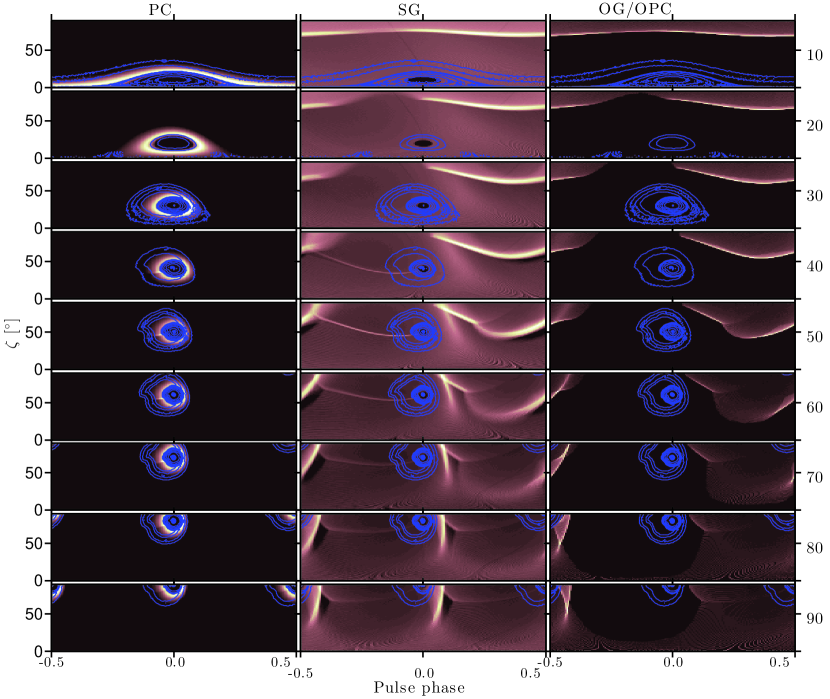
Appendix C Recurrence of $\gamma$-ray and radio shape classes

	PC		SG		OG		OPC
	$D$	$p_{\mathrm{value}}$ [%]	$D$	$p_{\mathrm{value}}$ [%]	$D$	$p_{\mathrm{value}}$ [%]	$D$	$p_{\mathrm{value}}$ [%]
Fig. 16: Radio peak multiplicity distribution	0.42	3e-8	gray!600.37	gray!605e-6	0.45	1e-9	gray!300.417	gray!304e-8
Fig. 17-left: RQ $\gamma$-ray peak multiplicity distribution	0.72	2.4	0.38	2e-2	gray!300.17	gray!3033	gray!600.05	gray!6099.9
Fig. 17-right: RL $\gamma$-ray peak multiplicity distribution	gray!300.36	gray!301.8	0.35	6e-3	0.41	1e-4	gray!600.22	gray!602.6
Fig. 18-left: RQ shape-classes distribution	0.72	2.4	0.38	2e-2	gray!600.17	gray!6033	gray!300.18	gray!3024
Fig. 18-right: RL shape-classes distribution	gray!600.36	gray!601.8	gray!300.40	gray!303e-4	0.59	2e-11	0.56	2e-10

Table 8: Two-sample Kolmogorov-Smirnov statistics (2KS) and relative $p_{\mathrm{value}}$ between observed and simulated one-dimensional distributions shown in Figures 16 to 18 and each model. The 2KS statistics ranges between 0 and 1 for distributions showing total agreement and total disagreement, respectively. The $p_{\mathrm{value}}$ is the probability to obtain observed 2KS value under the assumption that the two distributions are obtained from the same distribution (null hypothesis). This is equivalent to reject the null hypothesis at a confidence level of 100-($p_{\mathrm{value}}$). The 2KS test is described in Section E. The $D$ parameters relative to the first and second most consistent distributions are highlighted in dark grey and light grey cells, respectively

Figure 16 compares simulated and observed multiplicities of $\gamma$-ray-selected radio profiles in the framework of each model. The radio model is unique, but the RL pulsars subsample changes with each model $\gamma$-ray visibility generating different radio-peak multiplicity distributions. Figure 17 compares simulated and observed $\gamma$-ray peak multiplicity for RQ and RL pulsars in the framework of each model. Figure 18 compares the recurrence of the shape classes defined in Tables 2 and 3 and shown in Tables 6 and 7 for the simulated $\gamma$-ray and radio pulsars, respectively. The statistical agreement between observed and simulated one-dimensional distributions shown in Figures 16 to 18 are listed in Table 8.

Figure 16: Recurrence of peak multiplicities for the simulated radio pulsar populations (grey) and LAT population (red) and each model. The radio peak multiplicities are defined in Table 6.

Figure 17: Recurrence of the $\gamma$-ray peak multiplicity for the RQ and RL pulsars of simulated (grey) and observed (red) populations and each model are shown in the top and bottom panels, respectively.

Figure 18: Recurrence shape classes for simulated $\gamma$-ray and radio pulsar populations (grey) and LAT population (red) and each model are shown in the top and bottom panel, respectively.

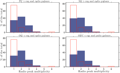
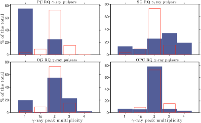
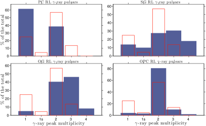
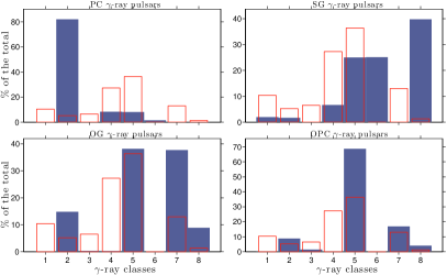
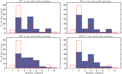
Appendix D Multiplicities and peak separations as a function of $P$ and $w$ in the $\alpha$-$\zeta$ plane

Figure 19: Peak multiplicity as a function of spin period (PC) and gap width (SG, OG, OPC) in the $\alpha$-$\zeta$ plane. Left to right columns refer to PC, SG, OG, and OPC, respectively while top to bottom rows refer to increasing period (PC) and gap width (SG, OG, OPC). This figure can be compared with similar figures of Watters et al. (2009).

Figure 20: Peak separation as a function of spin period (PC) and gap width (SG, OG, OPC) in the $\alpha$-$\zeta$ plane. Left to right columns refer to PC, SG, OG, and OPC, respectively while top to bottom rows refer to increasing period (PC) and gap width (SG, OG, OPC). This figure can be compared with similar figures of Watters et al. (2009).

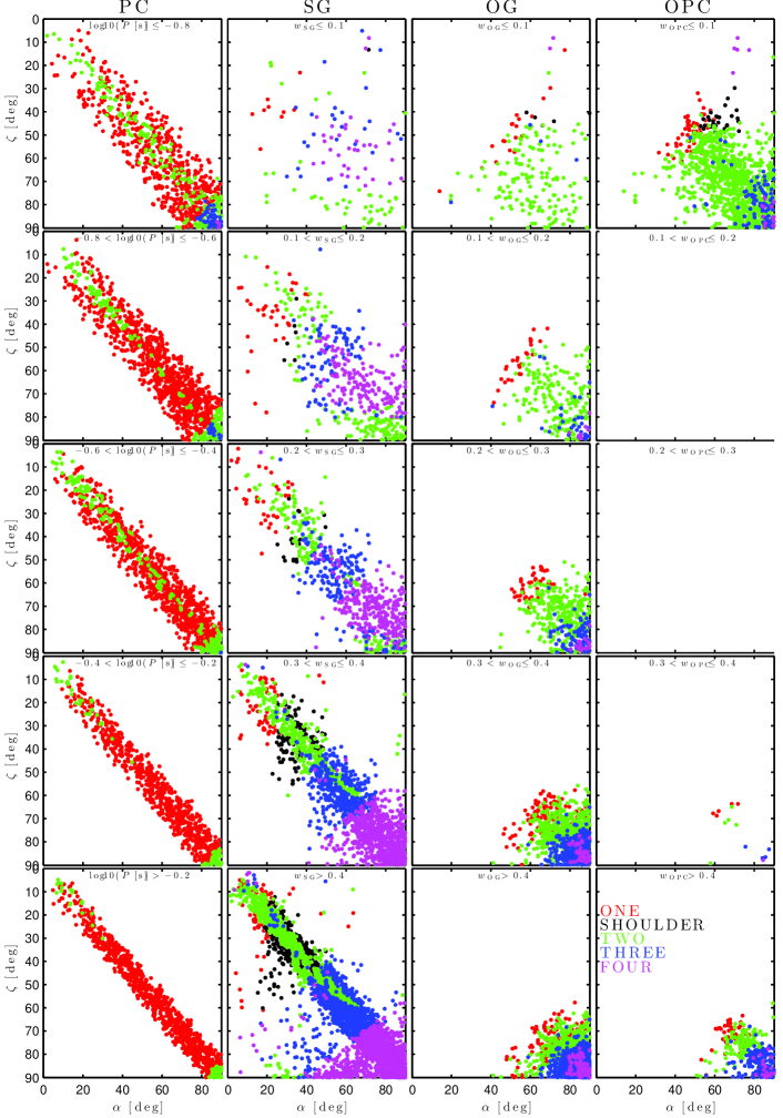
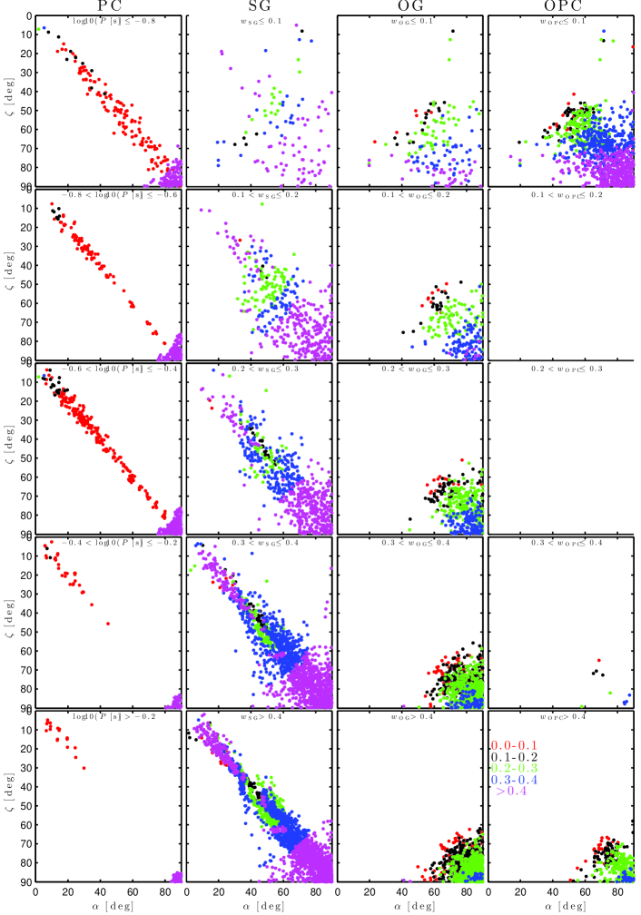
Appendix E Two-sample Kolmogorov-Smirnov test

The two-sample Kolmogorov-Smirnov test (2KS) is a non-parametric test that allows statistical quantification of the degree of agreement of two one-dimensional distributions. By computing the maximum distance between the cumulative density functions (CDFs) of the tested distributions, the 2KS test allows for the rejection of the null hypothesis: that the distributions are obtained from the same underlying distribution at a predefined confidence level (CL). We consider two samples, $A$ and $B$, of sizes $a$ and $b$, respectively. If $A(x)$ and $B(x)$ are the CDF of the samples A and B, respectively, the 2KS statistics is given by

$$D_{a,b}=\sup_{x}|A(x)-B(x)|$$ (1)

where $\sup$ is the supremium function. The null hypothesis that the samples A and B have been obtained from the same underlying distribution is rejected at CL $p_{\mathrm{value}}$ if

$$D_{a,b}>c(p_{\mathrm{value}})\sqrt{\frac{a+b}{ab}}$$ (2)

with $c(p_{\mathrm{value}})$ a tabulated value function of the chosen CL. The D value is included between 0 and 1 indicating total agreement and total disagreement between the tested distributions, respectively. The $p_{\mathrm{value}}$ gives the probability to observe the relative statistics $D_{a,b}$ assuming the null hypothesis to be true. The 2KS statistic and $p_{\mathrm{value}}$ given in Table 4 and relative to one-dimension observed and simulated distributions shown in Figures 4 to 6 have been computed with Equations 1 and 1, respectively.

E.1 Using the 2KS to quantify the agreement between two two-dimensional distributions

We used the two-dimensional version of the 2KS statistics (2D-2KS) described in Press et al. (1992) to quantify the agreement between observed/estimated and simulated two-dimensional distributions shown in Figures 7 to 13. The 2D-2KS statistics described in Press et al. (1992) gives a reasonable estimate of the distance between simulated and observed 2D distributions but, given the high number of possible ways to sort the 2D data plane, the 2D-2KS statistics is not distribution free as its 1D version, and cannot be associated with the probability that observations and simulations are obtained from the same parent distribution ($p_{\mathrm{value}}$). In order to evaluate the $p_{\mathrm{value}}$ associated with the 2D-2KS statistics, we studied the statistical distribution of the 2D-2KS statistics by paired bootstrap resampling of the observed 2D sample, and use it to evaluate the $p_{\mathrm{value}}$ corresponding to each 2D-2KS statistics.

The paired bootstrap resampling consists in resampling the observed 2D distribution by randomly rearrange the observed values on the 2D plane. It is possible to build a high number of bootstrapped distribution, statistically consistent with the observed 2D distribution, and use them to study the statistical distribution of a parameter of the observed 2D distribution (e.g. the variance). An accurate description of the paired bootstrap resampling can be found in Babu & Rao (1993).

We used the paired bootstrap method to resample each observed 2D distribution and create a large number of bootstrapped samples. We computed the 2D-2KS statistics between each bootstrapped sample and the simulated sample in object, and we built the statistical distribution of their 2D-2KS statistics for each model. Once we evaluated the statistical distribution of the 2D-2KS statistics, we used it to read off the probability $p_{\mathrm{value}}$ corresponding to the 2D-2KS statistics computed between the simulated and observed/estimated 2D distribution in the object.