Dynamical Selection of Critical Exponents

Kay Jörg Wiese CNRS-Laboratoire de Physique Théorique de l’Ecole Normale Supérieure, 24 rue Lhomond, 75005 Paris, France, PSL Research University, 62 bis Rue Gay-Lussac, 75005 Paris, France.
Abstract

In renormalized field theories there are in general one or few fixed points that are accessible by the renormalization-group flow. They can be identified from the fixed-point equations. Exceptionally, an infinite family of fixed points exists, parameterized by a scaling exponent ζ𝜁\zeta, itself function of a non-renormalizing parameter. Here we report a different scenario with an infinite family of fixed points of which seemingly only one is chosen by the renormalization-group flow. This dynamical selection takes place in systems with an attractive interaction 𝒱(ϕ)𝒱italic-ϕ{\cal V}(\phi), as in standard ϕ4superscriptitalic-ϕ4\phi^{4} theory, but where the potential 𝒱𝒱\cal V at large ϕitalic-ϕ\phi goes to zero, as e.g. the attraction by a defect.

I Introduction

The renormalzation group (RG) is a powerful tool to study critical phenomena of all sorts, be it liquid-gas transitions, the para to ferro transition in magnets, or disordered systems. In many cases one can identify a single or few relevant couplings, and study the RG-flow projected onto this space. An example is the famous ϕ4superscriptitalic-ϕ4\phi^{4} theory, whose coupling constant g𝑔g evolves under a change of an infrared scale m𝑚m. This framework is well understood. Originally introduced by Wilson WilsonKogut1974 , it has been treated in many excellent monographs BrezinBook ; Zinn ; CardyBook ; Amit .

Under more general circumstances, a functional RG approach is necessary. Let us start from a microscopic theory with action (energy), in the presence of a source (or background field) u𝑢u,

𝒮u[ϕ]=ddx12[ϕ(x)]2+m22[ϕ(x)u]2+𝒱0(ϕ).subscript𝒮𝑢delimited-[]italic-ϕsuperscriptd𝑑𝑥12superscriptdelimited-[]italic-ϕ𝑥2superscript𝑚22superscriptdelimited-[]italic-ϕ𝑥𝑢2subscript𝒱0italic-ϕ{\cal S}_{u}[\phi]=\int\mathrm{d}^{d}x\,\frac{1}{2}\left[\nabla\phi(x)\right]^{2}+\frac{m^{2}}{2}\left[\phi(x)-u\right]^{2}+{\cal V}_{0}(\phi)\ . (1)

The partition function

𝒵[u]:=𝒟[ϕ]e𝒮u[ϕ]assign𝒵delimited-[]𝑢𝒟delimited-[]italic-ϕsuperscriptesubscript𝒮𝑢delimited-[]italic-ϕ{\cal Z}[u]:=\int{\cal D}[\phi]\mathrm{e}^{-{\cal S}_{u}[\phi]} (2)

explicitly depends on the source u𝑢u. To 1-loop order the partition function, evaluated at constant background field u𝑢u, and normalized with its counterpart at 𝒱=0𝒱0{\cal V}=0, reads

ln(𝒵[u]𝒵0[u])=Λddk(2π)dln(1+𝒱0′′(u)k2+m2).𝒵delimited-[]𝑢subscript𝒵0delimited-[]𝑢superscriptΛsuperscriptd𝑑𝑘superscript2𝜋𝑑1superscriptsubscript𝒱0′′𝑢superscript𝑘2superscript𝑚2\ln\!\left(\frac{{\cal Z}[u]}{{\cal Z}_{0}[u]}\right)=-\int^{\Lambda}\frac{\mathrm{d}^{d}k}{(2\pi)^{d}}\ln\!\left(1+\frac{{\cal V}_{0}^{\prime\prime}(u)}{k^{2}+m^{2}}\right)\ . (3)

We have explicitly written an UV cutoff ΛΛ\Lambda. This equation is at the origin of non-perturbative renormalization group schemes HazenfratzHasenfratz1968 ; WegnerHoughton1973 ; Polchinski1984 ; BergesTetradisWetterich2002 , (confusingly) also referred to as exact RG. To leading order, the effective action is Γ(u)=ln(𝒵[u]/𝒵0[u])Γ𝑢𝒵delimited-[]𝑢subscript𝒵0delimited-[]𝑢\Gamma(u)=-\ln\!({{\cal Z}[u]}/{{\cal Z}_{0}[u]}), and denoting its local part by 𝒱(u)𝒱𝑢{\cal V}(u), we arrive at the following functional flow equation for the renormalized potential 𝒱(u)𝒱𝑢{\cal V}(u)

mm𝒱(u)=mmΛddk(2π)dln(1+𝒱0′′(u)k2+m2).𝑚subscript𝑚𝒱𝑢𝑚subscript𝑚superscriptΛsuperscriptd𝑑𝑘superscript2𝜋𝑑1superscriptsubscript𝒱0′′𝑢superscript𝑘2superscript𝑚2-m\partial_{m}{\cal V}(u)=-m\partial_{m}\int^{\Lambda}\frac{\mathrm{d}^{d}k}{(2\pi)^{d}}\ln\!\left(1+\frac{{\cal V}_{0}^{\prime\prime}(u)}{k^{2}+m^{2}}\right)\ . (4)

To simplify the treatment, we restrict ourselves to perturbative RG, retaining only terms local in space. These are the terms of order 𝒱′′(u)superscript𝒱′′𝑢{\cal V}^{\prime\prime}(u), and [𝒱′′(u)]2superscriptdelimited-[]superscript𝒱′′𝑢2[{\cal V}^{\prime\prime}(u)]^{2}, leading to

Refer to caption
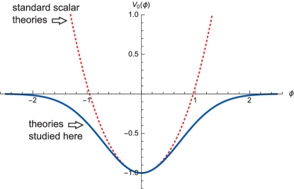
Figure 1: The function 𝒱0(ϕ)subscript𝒱0italic-ϕ{\cal V}_{0}(\phi), for ϕ4superscriptitalic-ϕ4\phi^{4} theory (top, red, dashed), and a bounded potential (bottom, blue, solid).
mm𝒱(u)𝑚subscript𝑚𝒱𝑢\displaystyle\!\!\!-m\partial_{m}{\cal V}(u)
=mmΛddk(2π)d[𝒱′′(u)k2+m212𝒱′′(u)2(k2+m2)2+].absent𝑚subscript𝑚superscriptΛsuperscriptd𝑑𝑘superscript2𝜋𝑑delimited-[]superscript𝒱′′𝑢superscript𝑘2superscript𝑚212superscript𝒱′′superscript𝑢2superscriptsuperscript𝑘2superscript𝑚22\displaystyle=-m\partial_{m}\int^{\Lambda}\!\!\frac{\mathrm{d}^{d}k}{(2\pi)^{d}}\left[\frac{{\cal V}^{\prime\prime}(u)}{k^{2}+m^{2}}\color[rgb]{0,0,0}-\frac{1}{2}\frac{{\cal V}^{\prime\prime}(u)^{2}}{(k^{2}+m^{2})^{2}}+...\right]\ .~{}~{}~{}~{}~{}~{}~{}~{} (5)

Taking the limit of ΛΛ\Lambda\to\infty, and dropping geometric prefactors, the flow equation becomes

mm𝒱(u)=md2𝒱′′(u)md412𝒱′′(u)2+.𝑚subscript𝑚𝒱𝑢superscript𝑚𝑑2superscript𝒱′′𝑢superscript𝑚𝑑412superscript𝒱′′superscript𝑢2-m\partial_{m}{\cal V}(u)={\color[rgb]{0,0,0}m^{d-2}{{\cal V}^{\prime\prime}(u)}}-m^{d-4}\frac{1}{2}{\cal V}^{\prime\prime}(u)^{2}+...\ . (6)

In the infrared (massless) limit we are interested in, the parameter m𝑚m becomes small, and the first term can be neglected as compared to the second one, leading to the simple flow equation

mm𝒱(u)=md412𝒱′′(u)2+.𝑚subscript𝑚𝒱𝑢superscript𝑚𝑑412superscript𝒱′′superscript𝑢2-m\partial_{m}{\cal V}(u)=-m^{d-4}\frac{1}{2}{\cal V}^{\prime\prime}(u)^{2}+...\ . (7)

This equation reproduces the standard RG-equation for the ϕ4superscriptitalic-ϕ4\phi^{4} theory; indeed, setting

𝒱(u)=m4du472g,𝒱𝑢superscript𝑚4𝑑superscript𝑢472𝑔{\cal V}(u)=m^{4-d}\frac{u^{4}}{72}\,g\ , (8)

we arrive with ε:=4dassign𝜀4𝑑\varepsilon:=4-d at

mmg=εgg2+.𝑚subscript𝑚𝑔𝜀𝑔superscript𝑔2-m\partial_{m}\,g=\varepsilon g-g^{2}+...\ . (9)

This is the standard flow equation of ϕ4superscriptitalic-ϕ4\phi^{4} theory, with fixed point g=εsubscript𝑔𝜀g_{*}=\varepsilon. One knows that the potential (8) at g=g𝑔subscript𝑔g=g_{*} is attractive, i.e. perturbing it with a perturbation ϕ2nsuperscriptitalic-ϕ2𝑛\phi^{2n}, n>2𝑛2n>2, the flow will bring it back to its fixed-point form.

This fixed point, and its treatment with the projected simplified flow equation (9) is relevant in many situations, the most famous being the Ising model. The form of its microscopic potential, which is plotted in figure 1 (red dashed curve), grows unboundedly for large ϕitalic-ϕ\phi. This is indeed expected for the Ising model, for which the spin, of which ϕitalic-ϕ\phi is the coarse-grained version, is bounded.

There are, however, situations, where this is not the case. An example is the attraction of a domain wall by a defect. In this situation, one expects that the potential at large ϕitalic-ϕ\phi vanishes, as plotted on figure 1 (solid blue line). The question to be asked is then: Where does the RG flow lead? This is the question addressed in this article.

As one sees from figure 1, the bounded potential 𝒱0subscript𝒱0{\cal V}_{0} is negative. In order to deal only with positive quantities, we set 𝒱(u)(u)𝒱𝑢𝑢{\cal V}(u)\equiv-{\cal R}(u). The flow equation to be studied is

mm(u)=mε12′′(u)2+.𝑚subscript𝑚𝑢superscript𝑚𝜀12superscript′′superscript𝑢2-m\partial_{m}{\cal R}(u)=m^{-\varepsilon}\frac{1}{2}{\cal R}^{\prime\prime}(u)^{2}+...\ . (10)

The potential (u)𝑢{\cal R}(u) appearing in this equation is not dimensionless. Similar to Eq. (8), we define a dimensionless function

R(u):=mε+4ζ(umζ).assign𝑅𝑢superscript𝑚𝜀4𝜁𝑢superscript𝑚𝜁R(u):=m^{-\varepsilon+4\zeta}{\cal R}(u\,m^{-\zeta})\ . (11)

Note that we have allowed for a non-trivial scaling dimension ζ𝜁\zeta of the field u𝑢u. The factor of m4ζsuperscript𝑚4𝜁m^{4\zeta} is necessary to compensate for the dimension of the derivatives. With these definitions, the flow equation reads

mmR(u)=(ε4ζ)R(u)+ζuR(u)+12R′′(u)2+.𝑚subscript𝑚𝑅𝑢𝜀4𝜁𝑅𝑢𝜁𝑢superscript𝑅𝑢12superscript𝑅′′superscript𝑢2-m\partial_{m}R(u)=(\varepsilon-4\zeta)R(u)+\zeta uR^{\prime}(u)+\frac{1}{2}R^{\prime\prime}(u)^{2}+...\ . (12)

Note that the RG parameter m𝑚m appearing in this equation has an intuitive physical interpretation: It is the curvature of the confining parabolic potential, which renders the problem well-defined.

In the remainder of this article, we will show that for generic smooth initial conditions as plotted on figure 1:

  1. (i)

    The flow equations (10) and (12) develop a cusp at u=0𝑢0u=0, and a cubic singularity at u=uc>0𝑢subscript𝑢𝑐0u=u_{c}>0.

  2. (ii)

    Eq. (12) has an infinity of solutions, indexed by ζ[ε4,]𝜁𝜀4\zeta\in[\frac{\varepsilon}{4},\infty].

  3. (iii)

    The solution chosen dynamically when starting from smooth initial conditions is ζ=ε3𝜁𝜀3\zeta=\frac{\varepsilon}{3}.

Refer to caption
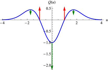
Figure 2: The function 𝒬(u)=′′(u21)eu2/2𝒬𝑢superscript′′superscript𝑢21superscriptesuperscript𝑢22{\cal Q}(u)={\cal R}^{\prime\prime}(u^{2}-1)\mathrm{e}^{-u^{2}/2}, and its flow at the maxima, minima and zeros.

II Some remarks on the literature

The problem considered here is far from new, and many articles have been written on the subject, under the denomination of “wetting”. The latter can be defined as preferential absorption of one component of a binary liquid by a wall. Let us summarize the situation:

  1. (i)

    Brezin, Halperin and Leibler BrezinHalperinLeibler1983a ; BrezinHalperinLeibler1983 identified d=3𝑑3d=3 as the critical dimension for wetting. They considered mean-field theory and perturbations around it. This analysis, as several following ones DSFisherHuse1985 ; BrezinHalpin-Healy1983 , is based on the linear term in the functional RG flow equation.

  2. (ii)

    Lipowsky and Fisher LipowskyFisher1987 , reviewed in Ref. ForgasLipowskyNieuwenhuizenInDombGreen , write down a functional RG equation similar111The flow equations (4.14) of LipowskyFisher1987 and (3.147) of ForgasLipowskyNieuwenhuizenInDombGreen contain a log, and not its derivative as our Eq. (4). The reason is that the flow w.r.t. the UV cutoff ΛΛ\Lambda is considered. Starting from Eq. (3) this yields instead of Eq. (4), and up to a multiplicative constant, ΛΛ𝒱(u)=Λdln(1+𝒱0′′(u)Λ2+m2).ΛsubscriptΛ𝒱𝑢superscriptΛ𝑑1superscriptsubscript𝒱0′′𝑢superscriptΛ2superscript𝑚2\Lambda\partial_{\Lambda}{\cal V}(u)={\Lambda}^{d}\ln\!\left(1+\frac{{\cal V}_{0}^{\prime\prime}(u)}{\Lambda^{2}+m^{2}}\right)\ . to our Eq. (4). While the analysis in the linear regime follows the same line of reasoning as Refs. BrezinHalperinLeibler1983a ; BrezinHalperinLeibler1983 ; DSFisherHuse1985 ; BrezinHalpin-Healy1983 , they also analyze the full non-linear flow equations. The fixed points found all contain a power-law tail, and diverge with a power law at small u𝑢u, or are repulsive. They are thus very different from the fixed points that we will discuss below, and to which a short-ranged initial condition will flow.

  3. (iii)

    Another possibility is to consider short-ranged potentials 𝒱(u)δ(u)similar-to-or-equals𝒱𝑢𝛿𝑢{\cal V}(u)\simeq\delta(u) from the start. This leads to a renormalizable field theory, pioneered by David, Duplantier and Guitter DDG1 ; DDG2 , and further studied by several authors LassigLipowsky1993 ; Wiese1996a ; PinnowWiese2001 ; PinnowWiese2002a ; PinnowWiese2004 . It is this approach that has been successful to tackle the renormalization of self-avoiding manifolds KardarNelson1987 ; AronowitzLubensky1987 ; DDG3 ; DDG4 ; WieseDavid1995 ; DavidWiese1996 ; WieseDavid1997 ; DavidWiese1998 ; DavidWiese2004 ; WieseHabil . As the potential 𝒱(u)𝒱𝑢{\cal V}(u) has been reduced to a δ𝛿\delta-function, any information contained in the shape of 𝒱(u)𝒱𝑢{\cal V}(u) is lost. While this approach is fully non-linear, its domain of applicability is restricted to repulsive potentials. (We consider attractive potentials.)
Refer to caption
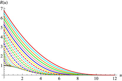
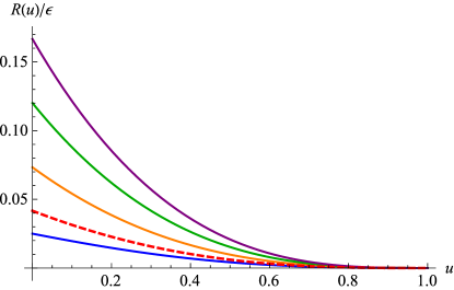
Figure 3: From bottom to top: Solutions for R(u)𝑅𝑢R(u) (divided by ε𝜀\varepsilon, or setting ε=1𝜀1\varepsilon=1) for uc=1subscript𝑢c1u_{\rm c}=1 and ζ=ε4𝜁𝜀4\zeta=\frac{\varepsilon}{4} (blue), ε3𝜀3\frac{\varepsilon}{3} (red, dashed), ε2𝜀2\frac{\varepsilon}{2} (orange), 3ε43𝜀4\frac{3\varepsilon}{4} (green) and ε𝜀\varepsilon (purple).

III Cusp formation

Define

:=1ε(mεm0ε),assign1𝜀superscript𝑚𝜀superscriptsubscript𝑚0𝜀\ell:=\frac{1}{\varepsilon}\Big{(}m^{-\varepsilon}-m_{0}^{-\varepsilon}\Big{)}\ , (13)

where m0subscript𝑚0m_{0} is the mass at which we start to integrate the RG equation. This leads to

(u)=12′′(u)2.subscript𝑢12superscript′′superscript𝑢2\partial_{\ell}{\cal R}(u)=\frac{1}{2}{\cal R}^{\prime\prime}(u)^{2}\ . (14)

Further define the curvature function

𝒬(u):=′′(u).assign𝒬𝑢superscript′′𝑢{\cal Q}(u):={\cal R}^{\prime\prime}(u)\ . (15)

It has flow equation

𝒬(u)=𝒬(u)𝒬′′(u)+𝒬(u)2.subscript𝒬𝑢𝒬𝑢superscript𝒬′′𝑢superscript𝒬superscript𝑢2\partial_{\ell}{\cal Q}(u)={\cal Q}(u){\cal Q}^{\prime\prime}(u)+{\cal Q}^{\prime}(u)^{2}\ . (16)

Let us integrate this flow equation from a microscopic (potentially already coarse-grained) potential =0(u)=eu2/2,subscript0𝑢superscriptesuperscript𝑢22{\cal R}_{\ell=0}(u)=\mathrm{e}^{-u^{2}/2}, i.e. 𝒬=0(u)=(u21)eu2/2.subscript𝒬0𝑢superscript𝑢21superscriptesuperscript𝑢22{\cal Q}_{\ell=0}(u)=(u^{2}-1)\mathrm{e}^{-u^{2}/2}. This function, plotted on Fig. 2, is negative for 0<u<u0=10𝑢subscript𝑢010<u<u_{0}=1, and positive for u>u0𝑢subscript𝑢0u>u_{0}. It has a zero with linear slope at u0=±1subscript𝑢0plus-or-minus1u_{0}=\pm 1. According to Eq. (16)

𝒬(u0)=𝒬(u0)2>0,subscript𝒬subscript𝑢0superscript𝒬superscriptsubscript𝑢020\partial_{\ell}{\cal Q}(u_{0})={\cal Q}^{\prime}(u_{0})^{2}>0\ , (17)

and the point u0subscript𝑢0u_{0} will move towards 00.

Q(u)𝑄𝑢Q(u) further has a minimum at umin=0subscript𝑢min0u_{\rm min}=0 and maxima at umax=±3subscript𝑢maxplus-or-minus3u_{\rm max}=\pm\sqrt{3}. Again according to Eq. (16), for u=umin𝑢subscript𝑢minu=u_{\rm min} or u=umax𝑢subscript𝑢maxu=u_{\rm max},

𝒬(u)=𝒬(u)𝒬′′(u)<0.subscript𝒬𝑢𝒬𝑢superscript𝒬′′𝑢0\partial_{\ell}{\cal Q}(u)={\cal Q}(u){\cal Q}^{\prime\prime}(u)<0\ . (18)

Thus both the minimum and the maxima will decrease.

Since 𝒬(u)𝒬𝑢{\cal Q}(u) is a second derivative of an asymptotically vanishing function, it integrates to 0,

du𝒬(u)=0.superscriptsubscriptdifferential-d𝑢𝒬𝑢0\int_{-\infty}^{\infty}\mathrm{d}u\,{\cal Q}(u)=0\ . (19)

These observations combined imply that u00subscript𝑢00u_{0}\to 0, and that 𝒬(u)𝒬𝑢{\cal Q}(u) must develop a δ𝛿\delta-function singularity at u=0𝑢0u=0. Denoting

𝒬0:=limu00u0u0duQ(u),assignsubscript𝒬0subscriptsubscript𝑢00superscriptsubscriptsubscript𝑢0subscript𝑢0differential-d𝑢𝑄𝑢{\cal Q}_{0}:=\lim_{u_{0}\to 0}\int_{-u_{0}}^{u_{0}}\mathrm{d}u\,Q(u)\ , (20)

we can decompose the function 𝒬(u)𝒬𝑢{\cal Q}(u) into a regular and a singular part,

𝒬(u)=𝒬0δ(u)+𝒬reg(u).𝒬𝑢subscript𝒬0𝛿𝑢subscript𝒬reg𝑢{\cal Q}(u)={\cal Q}_{0}\delta(u)+{\cal Q}_{\rm reg}(u)\ . (21)

For the function (u)𝑢{\cal R}(u) it implies a cusp at u=0𝑢0u=0, with (0+)=𝒬0/2superscriptsuperscript0subscript𝒬02{\cal R}^{\prime}(0^{+})={\cal Q}_{0}/2.

Refer to caption
Figure 4: Early stages in the development of R(u)𝑅𝑢R(u), starting from the initial configuration R(u)=eu2/8𝑅𝑢superscriptesuperscript𝑢28R(u)=\mathrm{e}^{-u^{2}/8} (black solid line); subsequent configurations have a larger value of R(0R(0). The first seven (dotted) configurations are almost at the same time, for the remaining configurations ti1/3superscriptsubscript𝑡𝑖13t_{i}^{1/3} grows linearly. Curves are drawn after 1/δt1𝛿𝑡1/\delta t iterations, for a total of 21/δt21𝛿𝑡21/\delta t iterations. The last configuration is close to the fixed point with ζ=ε/3𝜁𝜀3\zeta=\varepsilon/3.

Refer to caption       Refer to caption

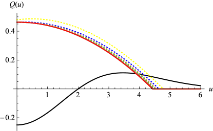
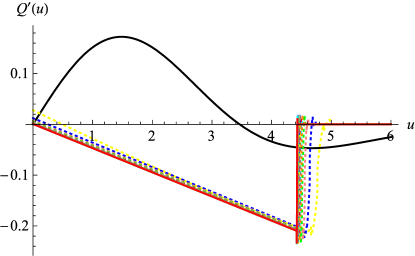
Figure 5: Q(u)𝑄𝑢Q(u) and Q(u)superscript𝑄𝑢Q^{\prime}(u) as obtained from the numerical integration of the flow equation, rescaled with ζ/ε=1/3𝜁𝜀13{\zeta/\varepsilon}=1/3. (Thus the axes are u1/3𝑢superscript13u\ell^{-1/3}, as well as Q1/3𝑄superscript13Q\ell^{1/3} and Q2/3superscript𝑄superscript23Q^{\prime}\ell^{2/3}.) The initial condition is in black, followed by 21 temporal snapshots, from yellow dashed (the rightmost curves on both plots) to solid red (left-most curve). One sees how Q𝑄Q converges to an inverted parabola, and Qsuperscript𝑄Q^{\prime} to a straight line with 𝒬(0+)=0superscript𝒬superscript00{\cal Q}^{\prime}(0^{+})=0. The overshoot in the plots for Q(u)superscript𝑄𝑢Q^{\prime}(u) are numerical artifacts.

IV A family of fixed points

We now search fixed points of Eq. (12). We are looking for solutions of

(ε4ζ)R(u)+ζuR(u)+12R′′(u)2=0.𝜀4𝜁𝑅𝑢𝜁𝑢superscript𝑅𝑢12superscript𝑅′′superscript𝑢20(\varepsilon-4{\zeta})R(u)+{\zeta}uR^{\prime}(u)+\frac{1}{2}R^{\prime\prime}(u)^{2}=0\ . (22)

We found an infinite family of fixed points, parameterized by the exponent ζ𝜁{\zeta}. Some examples are given on Fig. 3. They all have a linear cusp at u=0𝑢0u=0; their Taylor-expansion around uc=1subscript𝑢c1u_{\rm c}=1 starts with a cubic term,

R(u)𝑅𝑢\displaystyle\!\!\!\!R(u) =\displaystyle= ζ6(1u)3+ζε48(1u)4𝜁6superscript1𝑢3𝜁𝜀48superscript1𝑢4\displaystyle\frac{{\zeta}}{6}(1-u)^{3}+\frac{{\zeta}-\varepsilon}{48}(1-u)^{4}
+(εζ)(3ζε)1440ζ(1u)5𝜀𝜁3𝜁𝜀1440𝜁superscript1𝑢5\displaystyle+\frac{(\varepsilon-{\zeta})(3{\zeta}-\varepsilon)}{1440{\zeta}}(1-u)^{5}
+(ζε)(3ζ2ε)(3ζε)17280ζ2(1u)6+𝜁𝜀3𝜁2𝜀3𝜁𝜀17280superscript𝜁2superscript1𝑢6\displaystyle+\frac{({\zeta}-\varepsilon)(3{\zeta}-2\varepsilon)(3{\zeta}-\varepsilon)}{17280{\zeta}^{2}}(1-u)^{6}+... (23)

For u>1𝑢1u>1, it vanishes, R(u)=0𝑅𝑢0R(u)=0. For u<0𝑢0u<0, it satisfies R(u)=R(|u|)𝑅𝑢𝑅𝑢R(u)=R(|u|). We found the following analytic solutions, valid for 0u10𝑢10\leq u\leq 1:

Rζ=ε4(u)subscript𝑅𝜁𝜀4𝑢\displaystyle R_{{\zeta}=\frac{\varepsilon}{4}}(u) =\displaystyle= ε[2u5/245u472u18+140],𝜀delimited-[]2superscript𝑢5245superscript𝑢472𝑢18140\displaystyle\varepsilon\left[\frac{2u^{5/2}}{45}-\frac{u^{4}}{72}-\frac{u}{18}+\frac{1}{40}\right]\ , (24)
Rζ=ε3(u)subscript𝑅𝜁𝜀3𝑢\displaystyle R_{{\zeta}=\frac{\varepsilon}{3}}(u) =\displaystyle= ε[118(1u)3172(1u)4],𝜀delimited-[]118superscript1𝑢3172superscript1𝑢4\displaystyle\varepsilon\left[\frac{1}{18}(1-u)^{3}-\frac{1}{72}(1-u)^{4}\right]\ , (25)
Rζ=ε(u)subscript𝑅𝜁𝜀𝑢\displaystyle R_{{\zeta}=\varepsilon}(u) =\displaystyle= ε6(1u)3.𝜀6superscript1𝑢3\displaystyle\frac{\varepsilon}{6}(1-u)^{3}\ . (26)

The Taylor expansion around uc=1subscript𝑢c1u_{\rm c}=1, for which the first terms are displayed in Eq. (IV), converges for ζ>ε4𝜁𝜀4\zeta>\frac{\varepsilon}{4}. At ζ=ε4𝜁𝜀4\zeta=\frac{\varepsilon}{4} the function R(u)𝑅𝑢R(u) develops an additional singularity at u=0𝑢0u=0, and there seems to be no solution222The convergence radius of the Taylor expansion around 1 is finite, but smaller than 1 for ζ<ε4𝜁𝜀4\zeta<\frac{\varepsilon}{4}. for ζ<ε4𝜁𝜀4\zeta<\frac{\varepsilon}{4}.

V Numerical integration of the flow-equations, and fixed-point selection

We now integrate numerically the flow equation (14). We solve this equation by discretization in space u𝑢u and “time” \ell. Several technical problems need to be considered: First of all, after developing a cusp, the derivative ′′(0)superscript′′0{\cal R}^{\prime\prime}(0) no longer exists. To integrate the flow equations, we define

′′(0):=limu0′′(u).assignsuperscript′′0subscript𝑢0superscript′′𝑢{\cal R}^{\prime\prime}(0):=\lim_{u\to 0}{\cal R}^{\prime\prime}(u)\ . (27)

This limit is obtained by evaluating the discrete second derivative

′′(u)=(u+δu)+(uδu)2(u)(δu)2superscript′′𝑢𝑢𝛿𝑢𝑢𝛿𝑢2𝑢superscript𝛿𝑢2{\cal R}^{\prime\prime}(u)=\frac{{\cal R}(u+\delta u)+{\cal R}(u-\delta u)-2{\cal R}(u)}{(\delta u)^{2}} (28)

on grid points 2 to 10, and then extrapolating to the first point with the help of a cubic extrapolation.

As this procedure seems to be slightly arbitrary, the following reflection is useful: Instead of making the analysis on the function (u)𝑢{\cal R}(u), we can perform it on the function (|u|)𝑢{\cal R}(|u|), defined on the interval u[0,]𝑢0u\in[0,\infty]. Derivatives are defined for u]0,]u\in]0,\infty]. The natural boundary conditions at u=0𝑢0u=0 are Neumann boundary conditions. This parametrization is natural at large N𝑁N, see section VIII.1.

Second, in order to accelerate the calculations and ensure numerical stability, we iterate

+δ(u)subscript𝛿𝑢\displaystyle{\cal R}_{\ell+\delta\ell}(u) =\displaystyle= (u)+δ2′′(u)2,subscript𝑢𝛿2superscript′′superscript𝑢2\displaystyle{\cal R}_{\ell}(u)+\frac{\delta\ell}{2}{\cal R}^{\prime\prime}(u)^{2}\ , (29)
δsubscript𝛿\displaystyle\delta_{\ell} =\displaystyle= δtmaxu{′′(u)2}.𝛿𝑡subscript𝑢superscript′′superscript𝑢2\displaystyle\frac{\delta t}{\max_{u}\{{\cal R}^{\prime\prime}(u)^{2}\}}\ . (30)

The parameters chosen were δu=0.2𝛿𝑢0.2\delta u=0.2, and δt=104𝛿𝑡superscript104\delta t=10^{-4}. The result, plotted as a function of u1/3𝑢superscript13u\ell^{-1/3}, is shown on Fig. 4. The last curve, properly rescaled, is very close to the analytically obtained solution for ζ=ε3𝜁𝜀3\zeta=\frac{\varepsilon}{3}; this is even better seen on the derivatives plotted on figure 5. That this solution is attained can be checked with several indicators:

First, making the ansatz (u)=f()Rζ(g()u)subscript𝑢𝑓subscript𝑅𝜁𝑔𝑢{\cal R}_{\ell}(u)=f(\ell)\,R_{\zeta}\big{(}g(\ell)u\big{)}, inserting into the flow equation (14) and using the fixed point condition (12) yields

εζ=4+f()g()f()g().𝜀𝜁4superscript𝑓𝑔𝑓superscript𝑔\frac{\varepsilon}{\zeta}={4+\frac{f^{\prime}(\ell)g(\ell)}{f(\ell)g^{\prime}(\ell)}}\ . (31)

Both f()𝑓f(\ell) and g()𝑔g(\ell) can be measured with high precision, the first from the value of (0)0{\cal R}(0), the second from an estimation of the singular point ucsubscript𝑢cu_{\rm c}.

Three other functions depending on ζ𝜁\zeta can be calculated from the fixed-point solution obtained above, and inverted to give ζ𝜁\zeta:

e1(ζ)subscript𝑒1𝜁\displaystyle e_{1}(\zeta) =\displaystyle= (0)′′′(uc)uc3,0superscript′′′subscript𝑢csuperscriptsubscript𝑢c3\displaystyle\frac{{\cal R}(0)}{{\cal R}^{\prime\prime\prime}(u_{\rm c})u_{\rm c}^{3}}\ , (32)
e2(ζ)subscript𝑒2𝜁\displaystyle e_{2}(\zeta) =\displaystyle= (0)(0)uc,0superscript0subscript𝑢c\displaystyle\frac{{\cal R}(0)}{{\cal R}^{\prime}(0)u_{\rm c}}\ , (33)
e3(ζ)subscript𝑒3𝜁\displaystyle e_{3}(\zeta) =\displaystyle= ′′(0)uc2(0).superscript′′0superscriptsubscript𝑢c20\displaystyle\frac{{\cal R}^{\prime\prime}(0)u_{\rm c}^{2}}{{\cal R}(0)}\ . (34)

The results from all four indicators are plotted on figure 6. They consistently show that the numerically obtained solution converges towards the solution with ζ=ε3𝜁𝜀3\zeta=\frac{\varepsilon}{3}.

Refer to caption
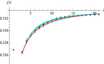
Figure 6: Approach to the fixed point for ζ=ε3𝜁𝜀3\zeta=\frac{\varepsilon}{3}, using different indicators, i.e. ζ𝜁\zeta extracted from R(0)/R′′′(uc)uc3𝑅0superscript𝑅′′′subscript𝑢csuperscriptsubscript𝑢c3R(0)/R^{\prime\prime\prime}(u_{\rm c})u_{\rm c}^{-3} (red), R(0)/R(0)uc1𝑅0superscript𝑅0superscriptsubscript𝑢c1R(0)/R^{\prime}(0)u_{\rm c}^{-1} (blue), R′′(0)/R(0)uc2superscript𝑅′′0𝑅0superscriptsubscript𝑢c2R^{\prime\prime}(0)/R(0)u_{\rm c}^{2} (green), and Eq. (31) (cyan). The index i𝑖i is the number of iterations in units of 105superscript10510^{5}, and the RG-time is 77.4(i1)3similar-to-or-equals77.4superscript𝑖13\ell\simeq 77.4\,(i-1)^{3}.

All fixed-point solutions found above have, for u𝑢u close to ucsubscript𝑢cu_{\rm c}, the form

(u)𝒜[uc()u]αΘ(u<uc()),similar-to-or-equalssubscript𝑢𝒜superscriptdelimited-[]subscript𝑢c𝑢𝛼Θ𝑢subscript𝑢c{\cal R}_{\ell}(u)\simeq{\cal A}\,[u_{\rm c}(\ell)-u]^{\alpha}\Theta\big{(}u<u_{\rm c}(\ell)\big{)}\ , (35)

with α=3𝛼3\alpha=3. This is understood as follows: Making the ansatz (35), and imposing the flow equation R(u,uc())=!12[u2R(u,uc())]2superscriptsubscript𝑅𝑢subscript𝑢c12superscriptdelimited-[]superscriptsubscript𝑢2𝑅𝑢subscript𝑢c2\partial_{\ell}R\big{(}u,u_{\rm c}(\ell)\big{)}\stackrel{{\scriptstyle!}}{{=}}\frac{1}{2}\left[\partial_{u}^{2}R\big{(}u,u_{\rm c}(\ell)\big{)}\right]^{2} implies

𝒜α[uc()u]α1uc()=!12[𝒜α(α1)]2[uc()u]2α4.superscript𝒜𝛼superscriptdelimited-[]subscript𝑢c𝑢𝛼1subscriptsubscript𝑢c12superscriptdelimited-[]𝒜𝛼𝛼12superscriptdelimited-[]subscript𝑢c𝑢2𝛼4{\cal A}\alpha\left[u_{\rm c}(\ell){-}u\right]^{\alpha-1}\partial_{\ell}u_{\rm c}(\ell)\stackrel{{\scriptstyle!}}{{=}}\frac{1}{2}\left[{\cal A}\alpha(\alpha{-}1)\right]^{2}\left[u_{\rm c}(\ell){-}u\right]^{2\alpha-4}. (36)

The same power-law on both sides is achieved for α=3𝛼3\alpha=3, which also gives the front velocity as

uc()=6𝒜.subscriptsubscript𝑢c6𝒜\partial_{\ell}\,u_{\rm c}(\ell)=6{\cal A}\ . (37)

We also remark that given ucsubscript𝑢cu_{\rm c}, the amplitude (0)0{\cal R}(0) is not fixed by the flow equation (14), even though it is fixed for the solutions of Eq. (22). Indeed, changing (u)κ(u)𝑢𝜅𝑢{\cal R}(u)\to\kappa{\cal R}(u), this can be absorbed into a change of κ𝜅\ell\to\kappa\ell. This is the reason why in Eqs. (32) to (34) all ratios are invariant under both a rescaling of {\cal R} and u𝑢u.

Refer to caption       Refer to caption

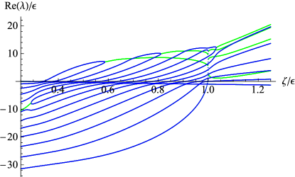
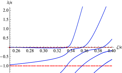
Figure 7: Left: The real part Re(λ)Re𝜆\mbox{Re}(\lambda) of the eigen-values of Eq. (38) in the space of polynomials up to degree 15. Real Eigen-values are shown in blue, complex pairs in green. Right: ibid, for n=24𝑛24n=24 for the five largest eigenvalues. The red points mark ζ=ε4𝜁𝜀4\zeta=\frac{\varepsilon}{4} and ζ=ε3𝜁𝜀3\zeta=\frac{\varepsilon}{3}. Note that the approximation for Rζ(u)subscript𝑅𝜁𝑢R_{\zeta}(u) is exact for ζ=ε3𝜁𝜀3\zeta=\frac{\varepsilon}{3} and ζ=ε𝜁𝜀\zeta=\varepsilon. The eigenmodes λ=0𝜆0\lambda=0 and λ=ε𝜆𝜀\lambda=-\varepsilon are given only approximately. Indeed, one can check that among the eigenfunctions of those eigenvalues close to 0 and 11-1 there is one each which strongly resembles the eigenfunctions (41) and (42). We interpret the errors as an effective level-repulsion induced by the truncation scheme. This error reduces only very slowly when going to higher orders.

VI Stability analysis

VI.1 General setting

Consider perturbations of Eq. (12) around a fixed point Rζsubscript𝑅𝜁R_{\zeta} with exponent ζ𝜁\zeta, setting R(u)=Rζ(u)+ηf(u)+𝑅𝑢subscript𝑅𝜁𝑢𝜂𝑓𝑢R(u)=R_{\zeta}(u)+\eta f(u)+.... Then, to linear order in η𝜂\eta, the flow for the perturbation f(u)𝑓𝑢f(u) is

mmf(u)=(ε4ζ)f(u)+ζuf(u)+f′′(u)Rζ′′(u).𝑚subscript𝑚𝑓𝑢𝜀4𝜁𝑓𝑢𝜁𝑢superscript𝑓𝑢superscript𝑓′′𝑢subscriptsuperscript𝑅′′𝜁𝑢-m\partial_{m}f(u)=(\varepsilon-4\zeta)f(u)+\zeta uf^{\prime}(u)+f^{\prime\prime}(u)R^{\prime\prime}_{\zeta}(u)\ . (38)

In general, we look for eigen-modes fλsubscript𝑓𝜆f_{\lambda} of the form

mmfλ(u)=λfλ(u).𝑚subscript𝑚subscript𝑓𝜆𝑢𝜆subscript𝑓𝜆𝑢-m\partial_{m}f_{\lambda}(u)=\lambda f_{\lambda}(u)\ . (39)

If we find fλ(u)subscript𝑓𝜆𝑢f_{\lambda}(u) with (λ)>0𝜆0\Re(\lambda)>0, then the fixed-point solution Rζ(u)subscript𝑅𝜁𝑢R_{\zeta}(u) is linearly unstable. Absence of such a solution does not necessarily allow to conclude linear stability; the stability matrix may, e.g. be non-diagonalizable.

VI.2 Stability of the solution with ζ=ε/3𝜁𝜀3\zeta=\varepsilon/3

We first establish the stability of the numerically chosen solution ζ=ε3𝜁𝜀3\zeta=\frac{\varepsilon}{3} w.r.t. higher-order polynomials. Setting f(u)=(1u)n𝑓𝑢superscript1𝑢𝑛f(u)=(1-u)^{n}, the r.h.s. of Eq. (38) becomes

mm(1u)n𝑚subscript𝑚superscript1𝑢𝑛\displaystyle-m\partial_{m}(1-u)^{n} =\displaystyle= ε[(n2)(n1)6(1u)n\displaystyle\varepsilon\bigg{[}-\frac{(n-2)(n-1)}{6}(1-u)^{n} (40)
(n2)n3(1u)n1].\displaystyle~{}~{}~{}~{}-\frac{(n-2)n}{3}(1-u)^{n-1}\bigg{]}\ .

This proves that the highest-order term, proportional to (1u)nsuperscript1𝑢𝑛(1-u)^{n} in the Taylor-expansion around 111 decays, and a subdominant one proportional to (1u)n1superscript1𝑢𝑛1(1-u)^{n-1} is generated. Finally, all terms with Taylor-coefficients larger than 222 are eliminated. Hence, the solution with ζ=ε3𝜁𝜀3\zeta=\frac{\varepsilon}{3} is linearly stable w.r.t. polynomial perturbations.

VI.3 Two exact eigen-modes

If Rζ(u)subscript𝑅𝜁𝑢R_{\zeta}(u) is a solution of the flow-equation, then η4Rζ(u/η)superscript𝜂4subscript𝑅𝜁𝑢𝜂\eta^{4}R_{\zeta}(u/\eta) also is a solution, implying that there is a marginal eigen-mode

f0(u)=η|η=1η4Rζ(u/η)=4Rζ(u)uRζ(u).subscript𝑓0𝑢evaluated-atsubscript𝜂𝜂1superscript𝜂4subscript𝑅𝜁𝑢𝜂4subscript𝑅𝜁𝑢𝑢superscriptsubscript𝑅𝜁𝑢f_{0}(u)=\partial_{\eta}\big{|}_{\eta=1}\eta^{4}R_{\zeta}(u/\eta)=4R_{\zeta}(u)-uR_{\zeta}^{\prime}(u)\ . (41)

Another eigenvector exists for λ=ε𝜆𝜀{\lambda=-\varepsilon}, as can be verified directly333It can be constructed from a superposition of the RG-fixed point and the marginal eigen-vector, see section VII.B of LeDoussalWiese2003a , where the twice derived form is given.

fε(u)=(ε4ζ)R(u)+ζuR(u).subscript𝑓𝜀𝑢𝜀4𝜁𝑅𝑢𝜁𝑢superscript𝑅𝑢f_{-\varepsilon}(u)=(\varepsilon-4\zeta)R(u)+\zeta uR^{\prime}(u)\ . (42)

VI.4 Stability analysis for generic values of ζ𝜁\zeta

Now consider ζε3𝜁𝜀3\zeta\neq\frac{\varepsilon}{3}. The flow of a perturbation proportional to (1u)nsuperscript1𝑢𝑛(1{-}u)^{n} then becomes

mm(1u)n𝑚subscript𝑚superscript1𝑢𝑛\displaystyle-m\partial_{m}(1{-}u)^{n} =\displaystyle= (ζε)(3ζ2ε)(3ζε)(n1)n576ζ2(1u)n+2𝜁𝜀3𝜁2𝜀3𝜁𝜀𝑛1𝑛576superscript𝜁2superscript1𝑢𝑛2\displaystyle\frac{(\zeta{-}\varepsilon)(3\zeta{-}2\varepsilon)(3\zeta{-}\varepsilon)(n{-}1)n}{576\zeta^{2}}(1{-}u)^{n+2} (43)
+(ζε)(3ζε)(1n)n72ζ(1u)n+1𝜁𝜀3𝜁𝜀1𝑛𝑛72𝜁superscript1𝑢𝑛1\displaystyle+\frac{(\zeta{-}\varepsilon)(3\zeta{-}\varepsilon)(1{-}n)n}{72\zeta}(1{-}u)^{n+1}
+(14(ζε)(n1)n+ζn+ε4ζ)(1u)n14𝜁𝜀𝑛1𝑛𝜁𝑛𝜀4𝜁superscript1𝑢𝑛\displaystyle+\!\left(\frac{1}{4}(\zeta{{-}}\varepsilon)(n{{-}}1)n{+}\zeta n{+}\varepsilon{{-}}4\zeta\right)(1{-}u)^{n}
+(n2)nζ(1u)n1].\displaystyle+(n{-}2)n\zeta(1{-}u)^{n-1}\bigg{]}\ .

First note that the space spanned by {1,1u}11𝑢\{1,1-u\} has no non-linear terms, hence the rescaling terms lead to λ0=ε4ζ<0subscript𝜆0𝜀4𝜁0\lambda_{0}=\varepsilon-4\zeta<0, and λ1=ε3ζsubscript𝜆1𝜀3𝜁\lambda_{1}=\varepsilon-3\zeta. The latter is positive for ζ<ε3𝜁𝜀3\zeta<\frac{\varepsilon}{3}. It is however questionable whether these solutions are allowed by the boundary conditions.

Higher-order terms are generated for all values of ζ𝜁\zeta other than ζ=ε3𝜁𝜀3\zeta=\frac{\varepsilon}{3} or ζ=ε𝜁𝜀\zeta=\varepsilon, and these solutions are potentially unstable. The solution ζ=ε𝜁𝜀\zeta=\varepsilon does not produce terms of order (1u)n+2superscript1𝑢𝑛2(1-u)^{n+2} or (1u)n+1superscript1𝑢𝑛1(1-u)^{n+1}, but the coefficient of the term (1u)nsuperscript1𝑢𝑛(1-u)^{n} becomes ε(n3)𝜀𝑛3\varepsilon(n-3), i.e. these terms grow for n>3𝑛3n>3, contrary to the solution ζ=ε3𝜁𝜀3\zeta=\frac{\varepsilon}{3}, for which they decay. We can thus conclude that ζ=ε𝜁𝜀\zeta=\varepsilon is unstable.

The situation for generic values of ζ𝜁\zeta is delicate, as we will see in a moment: The strategy we followed was to construct for fixed ζ𝜁\zeta a Taylor expansion of Rζ(u)subscript𝑅𝜁𝑢R_{\zeta}(u) around uc=1subscript𝑢c1u_{\rm c}=1 up to order n𝑛n, starting at n=2𝑛2n=2 (the space n1𝑛1n\leq 1 discussed above decouples). We then solved the Eigenvalue problem (38) in the space of polynomials up to degree n𝑛n in (1u)1𝑢(1-u). For n=15𝑛15n=15 the result is plotted on figure 7 (left), along with a blow-up for n=24𝑛24n=24 (right). (These are the maximal values of n𝑛n to not induce significant numerical errors in the chosen range of ζ𝜁\zeta). As figure 7 shows, solutions with ζ>ε3𝜁𝜀3\zeta>\frac{\varepsilon}{3} are unstable. The domain with ε4ζε3𝜀4𝜁𝜀3\frac{\varepsilon}{4}\leq\zeta\leq\frac{\varepsilon}{3} is seemingly stable. Our analysis is, however, bugged with a truncation problem that does not disappear for larger n𝑛n: The exact eigenmodes λ=0𝜆0\lambda=0 and λ=ε𝜆𝜀\lambda=-\varepsilon can only be found approximatively in figure 7 (right), where they are indicated by red dashed lines. We interpret these findings in the sense that there is a strong level-repulsion between the eigenvalues, induced by the truncation. One can indeed check that the exact eigenfunctions (41) and (42) are close to eigenfunctions in the spectrum of eigen-perturbations, even though their eigenvalues are off.


VI.5 Perturbing the solution ζ=ε4𝜁𝜀4\zeta=\frac{\varepsilon}{4}

The solution ζ=ε4𝜁𝜀4\zeta=\frac{\varepsilon}{4} is special. It has a continuous spectrum of eigen-functions, given with λ¯:=λ/εassign¯𝜆𝜆𝜀\bar{\lambda}:=\lambda/\varepsilon by

fλ(u)subscript𝑓𝜆𝑢\displaystyle f_{\lambda}(u) =\displaystyle= Γ(76162516λ¯)Γ(162516λ¯+76)2F1(162516λ¯56,162516λ¯56;13;u3/2)Γ(13)Γ76162516¯𝜆Γsubscript162516¯𝜆762subscript𝐹1162516¯𝜆56162516¯𝜆5613superscript𝑢32Γ13\displaystyle\frac{\Gamma\left(\frac{7}{6}-\frac{1}{6}\sqrt{25-16\bar{\lambda}}\right)\Gamma\left(\frac{1}{6}\sqrt{25-16\bar{\lambda}}+\frac{7}{6}\right)\,_{2}F_{1}\left(-\frac{1}{6}\sqrt{25-16\bar{\lambda}}-\frac{5}{6},\frac{1}{6}\sqrt{25-16\bar{\lambda}}-\frac{5}{6};\frac{1}{3};u^{3/2}\right)}{\Gamma\left(\frac{1}{3}\right)} (44)
uΓ(116162516λ¯)Γ(162516λ¯+116)2F1(162516λ¯16,162516λ16;53;u3/2)Γ(53).𝑢Γ116162516¯𝜆Γsubscript162516¯𝜆1162subscript𝐹1162516¯𝜆16162516𝜆1653superscript𝑢32Γ53\displaystyle-\frac{u\Gamma\left(\frac{11}{6}-\frac{1}{6}\sqrt{25-16\bar{\lambda}}\right)\Gamma\left(\frac{1}{6}\sqrt{25-16\bar{\lambda}}+\frac{11}{6}\right)\,_{2}F_{1}\left(-\frac{1}{6}\sqrt{25-16\bar{\lambda}}-\frac{1}{6},\frac{1}{6}\sqrt{25-16\lambda}-\frac{1}{6};\frac{5}{3};u^{3/2}\right)}{\Gamma\left(\frac{5}{3}\right)}\ .\qquad

A similar continuous spectrum is seemingly found when numerically solving the eigenvalue problem around a numerically obtained solution Rζ(u)subscript𝑅𝜁𝑢R_{\zeta}(u). We suspect that this analysis is invalid, since we do not impose appropriate boundary conditions at u=0𝑢0u=0.

VI.6 Numerical stability analysis

Our numerical simulation seems to chose the fastest available stable solution, in accordance to general “wisdom” of non-linear systems; however the latter has never been proven.
Refer to caption
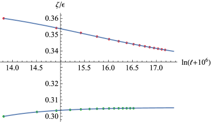
Figure 8: Estimation of ζ𝜁\zeta from the relation R(0)ucεζ4=!Rζ(0)superscriptsubscript𝑅0superscriptsubscript𝑢c𝜀𝜁4subscript𝑅𝜁0R_{\ell}(0)u_{\rm c}^{\frac{\varepsilon}{\zeta}-4}\stackrel{{\scriptstyle!}}{{=}}R_{\zeta}(0), starting from Rζ(u)subscript𝑅𝜁𝑢R_{\zeta}(u) with ζ=0.36ε𝜁0.36𝜀\zeta=0.36\varepsilon (top) and ζ=0.3ε𝜁0.3𝜀\zeta=0.3\varepsilon (bottom). The two fits are ζ()/ε=0.325118+5.04594(l+2.78605×106)0.33522𝜁𝜀0.3251185.04594superscript𝑙2.78605superscript1060.33522\zeta(\ell)/\varepsilon=0.325118\,+\frac{5.04594}{(l+2.78605\times 10^{6})^{0.33522}} (top), and ζ()/ε=0.3054285561.08l+1.02487×106𝜁𝜀0.3054285561.08𝑙1.02487superscript106\zeta(\ell)/\varepsilon=0.305428\,-\frac{5561.08}{l+1.02487\times 10^{6}} (bottom).

We tried to start from another fixed point in our family, and study whether it is stable when inserted into the flow equations and solved numerically. On figure 8 we show how starting from fixed-point solutions with ζ=0.3ε𝜁0.3𝜀\zeta=0.3\varepsilon (bottom) and ζ=0.36ε𝜁0.36𝜀\zeta=0.36\varepsilon (top) the RG flow evolves. While the solution with ζ>ε3𝜁𝜀3\zeta>\frac{\varepsilon}{3} seemingly converges towards the solution with ζ=ε3𝜁𝜀3\zeta=\frac{\varepsilon}{3}, this is not the case for the solution with ζ<ε3𝜁𝜀3\zeta<\frac{\varepsilon}{3}, in agreement with the stability analysis presented above. Note however, that even for ζ>ε3𝜁𝜀3\zeta>\frac{\varepsilon}{3} this convergence is on time scales that are orders of magnitude larger than the convergence from an analytic initial condition (see figure 6).

VII Higher-loop order

VII.1 The flow equations

At 2-loop order, we obtain the following functional renormalization group equation for the function R(u)𝑅𝑢R(u),

mmR(u)𝑚subscript𝑚𝑅𝑢\displaystyle-m\partial_{m}R(u) =\displaystyle= (ε4ζ)R(u)+ζuR(u)+12R′′(u)2𝜀4𝜁𝑅𝑢𝜁𝑢superscript𝑅𝑢12superscript𝑅′′superscript𝑢2\displaystyle(\varepsilon-4\zeta)R(u)+\zeta uR^{\prime}(u)+\textstyle\frac{1}{2}{R^{\prime\prime}(u)}^{2} (45)
+(12+ε𝒞1)R′′(u)R′′′(u)212𝜀subscript𝒞1superscript𝑅′′𝑢superscript𝑅′′′superscript𝑢2\displaystyle+\left({\textstyle\frac{1}{2}}+\varepsilon\,{\cal C}_{1}\right)R^{\prime\prime}(u){R^{\prime\prime\prime}(u)}^{2}
+𝒞2R′′′(u)4+𝒞3R′′(u)2R′′′′(u)2subscript𝒞2superscript𝑅′′′superscript𝑢4subscript𝒞3superscript𝑅′′superscript𝑢2superscript𝑅′′′′superscript𝑢2\displaystyle+{\cal C}_{2}{R^{\prime\prime\prime}(u)}^{4}+{\cal C}_{3}\,R^{\prime\prime}(u)^{2}{R^{\prime\prime\prime\prime}(u)}^{2}\rule{0.0pt}{12.91663pt}
+𝒞4R′′(u)R′′′(u)2R′′′′(u),subscript𝒞4superscript𝑅′′𝑢superscript𝑅′′′superscript𝑢2superscript𝑅′′′′𝑢\displaystyle+{\cal C}_{4}\,R^{\prime\prime}(u){R^{\prime\prime\prime}(u)}^{2}{R^{\prime\prime\prime\prime}(u)}\ ,\qquad\ \ \

with

𝒞1subscript𝒞1\displaystyle{\cal C}_{1} =\displaystyle= 14+π29ψ(13)6=0.335976809672364714superscript𝜋29superscript𝜓1360.3359768096723647\displaystyle\frac{1}{4}+\frac{\pi^{2}}{9}-\frac{\psi^{\prime}(\frac{1}{3})}{6}=-0.3359768096723647...~{}~{}~{} (46)
𝒞2subscript𝒞2\displaystyle{\cal C}_{2} =\displaystyle= 34ζ(3)+π218ψ(13)12=0.608554272533513134𝜁3superscript𝜋218superscript𝜓13120.6085542725335131\displaystyle\frac{3}{4}\zeta(3)+\frac{\pi^{2}}{18}-\frac{\psi^{\prime}(\frac{1}{3})}{12}=0.6085542725335131...~{}~{}~{}~{}~{}~{}~{}~{} (47)
𝒞3subscript𝒞3\displaystyle{\cal C}_{3} =\displaystyle= ψ(13)6π29=0.5859768096723648superscript𝜓136superscript𝜋290.5859768096723648\displaystyle\frac{\psi^{\prime}(\frac{1}{3})}{6}-\frac{\pi^{2}}{9}=0.5859768096723648... (48)
𝒞4subscript𝒞4\displaystyle{\cal C}_{4} =\displaystyle= 2+π29ψ(13)6=1.4140231903276352.2superscript𝜋29superscript𝜓1361.4140231903276352\displaystyle 2+\frac{\pi^{2}}{9}-\frac{\psi^{\prime}(\frac{1}{3})}{6}=1.4140231903276352...\ . (49)

The first line contains the rescaling and 1-loop terms, the second line the 2-loop terms, and the last two lines the three 3-loop terms. The constants are related by 𝒞1=14𝒞3subscript𝒞114subscript𝒞3\mathcal{C}_{1}=\frac{1}{4}-\mathcal{C}_{3}, and 𝒞4=2𝒞3=20.000190372subscript𝒞42subscript𝒞320.000190372{\cal C}_{4}=2-{\cal C}_{3}=\sqrt{2}-0.000190372...

Refer to caption
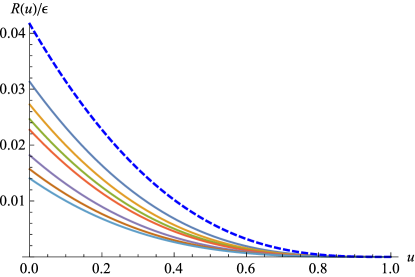
Figure 9: The 2-loop fixed point for ζ=ε3𝜁𝜀3\zeta=\frac{\varepsilon}{3}; at 1-loop order (blue dashed line), and 2-loop order for ε=0.25, 0.5, 0.75, 1, 2, 3, 4𝜀0.250.50.751234\varepsilon=0.25,\,0.5,\,0.75,\,1,\,2,\,3,\,4 (from top to bottom). The expansion is rather non-uniform.

VII.2 Problems with the ε𝜀\varepsilon expansion, and a consistent series for the 2-loop fixed point

Note that at 2-loop order, we get a term

12R′′(u)R′′′(u)2(1u)+similar-to12superscript𝑅′′𝑢superscript𝑅′′′superscript𝑢21𝑢\frac{1}{2}R^{\prime\prime}(u)R^{\prime\prime\prime}(u)^{2}\sim(1-u)+... (50)

close to the singularity when inserting any of our 1-loop solutions. Thus, there is no proper ε𝜀\varepsilon-expansion for the fixed point at higher order.

Valuable information is gained by studying the shock front generated by the flow-equation at n𝑛n-loop order. Without even calculating the Feynman diagrams, we conclude that

R(u,uc())!u4n[R(u,uc())]n+1.superscriptsimilar-to-or-equalssubscript𝑅𝑢subscript𝑢csuperscriptsubscript𝑢4𝑛superscriptdelimited-[]𝑅𝑢subscript𝑢c𝑛1\partial_{\ell}R\big{(}u,u_{\rm c}(\ell)\big{)}\stackrel{{\scriptstyle!}}{{\simeq}}\partial_{u}^{4n}\left[R\big{(}u,u_{\rm c}(\ell)\big{)}\right]^{n+1}\ . (51)

Supposing that

R(u,uc())𝒜[uc()u]α,similar-to-or-equals𝑅𝑢subscript𝑢c𝒜superscriptdelimited-[]subscript𝑢c𝑢𝛼R\big{(}u,u_{\rm c}(\ell)\big{)}\simeq{\cal A}\left[u_{\rm c}(\ell){-}u\right]^{\alpha}\ , (52)

the latter equation implies for the shock front

[uc()u]α1tuc()!𝒜n[uc()u](n+1)α4n.superscriptsimilar-to-or-equalssuperscriptdelimited-[]subscript𝑢c𝑢𝛼1subscript𝑡subscript𝑢csuperscript𝒜𝑛superscriptdelimited-[]subscript𝑢c𝑢𝑛1𝛼4𝑛\left[u_{\rm c}(\ell){-}u\right]^{\alpha-1}\partial_{t}u_{\rm c}(\ell)\stackrel{{\scriptstyle!}}{{\simeq}}{\cal A}^{n}\left[u_{\rm c}(\ell){-}u\right]^{(n+1)\alpha-4n}\ . (53)

This yields

α=41n.𝛼41𝑛\alpha=4-\frac{1}{n}\ . (54)

At 2-loop order, we should thus try an ansatz, starting at (1u)7/2superscript1𝑢72(1-u)^{7/2} instead of (1u)3superscript1𝑢3(1-u)^{3}. Indeed, such an ansatz is possible, resulting into the series expansion

R(u)𝑅𝑢\displaystyle{R(u)} =\displaystyle= 16ζ(1u)7/210552153(1u)416𝜁superscript1𝑢7210552153superscript1𝑢4\displaystyle\frac{16\sqrt{\zeta}(1-u)^{7/2}}{105\sqrt{5}}-\frac{2}{153}(1-u)^{4} (55)
+4(1u)9/2(26015ζ52025ε+15405)15566985ζ4superscript1𝑢9226015𝜁52025𝜀1540515566985𝜁\displaystyle+\frac{4(1-u)^{9/2}\left(2601\sqrt{5}\zeta-5202\sqrt{5}\varepsilon+1540\sqrt{5}\right)}{15566985\sqrt{\zeta}}
2(1u)5(223686ζ+200277ε45800)1323193725ζ2superscript1𝑢5223686𝜁200277𝜀458001323193725𝜁\displaystyle-\frac{2(1-u)^{5}(-223686\zeta+200277\varepsilon-45800)}{1323193725\zeta}
+\displaystyle+...

This series converges for all 0u10𝑢10\leq u\leq 1 as long as ε0.2𝜀0.2\varepsilon\geq 0.2. It is singular as a function of ε𝜀\varepsilon. This is shown on Fig. 9.

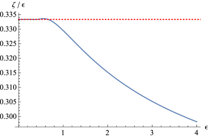
If we use the same selection criterion as at 1-loop order, namely that Q(0+)=R′′′(0+)=0superscript𝑄superscript0superscript𝑅′′′superscript00Q^{\prime}(0^{+})={R}^{\prime\prime\prime}(0^{+})=0, then this series expansion yields the exponents presented on figure 10. Curiously, when ε0.4𝜀0.4\varepsilon\leq 0.4, the exponent ζ/ε𝜁𝜀\zeta/\varepsilon does not change; it then increases slightly, before decreasing for larger values of ε𝜀\varepsilon.

Refer to caption
Figure 10: The exponent ζ𝜁\zeta as obtained from the criterion Q(0)=!0superscriptsuperscript𝑄00Q^{\prime}(0)\stackrel{{\scriptstyle!}}{{=}}0, using the series expansion for the 2-loop fixed point up to order (1u)15superscript1𝑢15(1-u)^{15}. Points between ε=0𝜀0\varepsilon=0 and ε=0.25𝜀0.25\varepsilon=0.25 have been replaced by a straight line, which continues on the numerically obtained plateau of unknown origin up to about ε=0.4𝜀0.4\varepsilon=0.4.

VII.3 Numerical integration of the flow-equations

We tried to confirm the above findings by a numerical integration of the flow-equations. Again we use discrete derivatives,

R′′(u)superscript𝑅′′𝑢\displaystyle R^{\prime\prime}(u) similar-to-or-equals\displaystyle\simeq R(u+δu)+R(uδu)2R(u)(δu)2𝑅𝑢𝛿𝑢𝑅𝑢𝛿𝑢2𝑅𝑢superscript𝛿𝑢2\displaystyle\frac{R(u{+}\delta u)+R(u{-}\delta u)-2R(u)}{(\delta u)^{2}} (56)
R′′′(u)superscript𝑅′′′𝑢\displaystyle\!\!R^{\prime\prime\prime}(u) similar-to-or-equals\displaystyle\simeq R(u+2δu)3R(u+δu)+3R(u)R(u+δu)(δu)3.𝑅𝑢2𝛿𝑢3𝑅𝑢𝛿𝑢3𝑅𝑢𝑅𝑢𝛿𝑢superscript𝛿𝑢3\displaystyle\frac{R(u{+}2\delta u)-3R(u{+}\delta u)+3R(u)-R(u{+}\delta u)}{(\delta u)^{3}}\ .

Note that the third derivative involves two points to the right, and only one to the left. For the point u=0𝑢0u=0, we take (as at 1-loop order) the first 4 points except the very first (i=2,3,4,5𝑖2345i=2,3,4,5) of the discrete derivative, and interpolate with a cubic polynomial, which is then extrapolated to i=1𝑖1i=1.

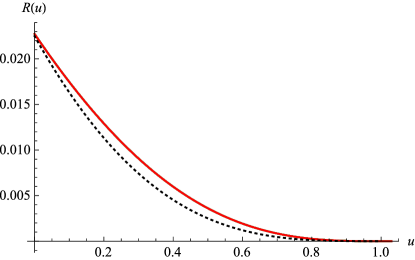
Our initial condition is the 1-loop solution for ζ=ε3𝜁𝜀3\zeta=\frac{\varepsilon}{3}, at ε=1𝜀1\varepsilon=1. We tried to use a smooth function to start with, but did not succeed to stabilize the system of equations. We have plotted the shape of the large-time solution on Fig. 11. It shows significant deviations from its 1-loop counterpart. We were not able to conclude on the asymptotic value of the exponent ζ𝜁\zeta. A stability analysis around the fixed-point solutions for ε=1𝜀1\varepsilon=1 yields results compatible with our 1-loop findings.
Refer to caption
Figure 11: The 2-loop fixed point R(u)𝑅𝑢R(u) at ε=1𝜀1\varepsilon=1, as obtained from a numerical integration of the flow equations (solid red), compared to the 1-loop fixed point (dashed, black). Both solutions were rescaled to have uc=1subscript𝑢c1u_{\rm c}=1, and R(0)=1/24𝑅0124R(0)=1/{24}.

VIII Related Models

VIII.1 Large N𝑁N, and relation to the KPZ equation

We now consider the generalizsation of our RG-equations to N𝑁N components, with the aim of taking the limit N𝑁N\to\infty. To this aim, we replace

(u)N(u22N).𝑢𝑁superscript𝑢22𝑁{\cal R}(u)\to N\,{\cal R}\!\left(\frac{\vec{u}^{2}}{2N}\right)\ . (58)

Taking into account the proper index structure, we arrive at the following (unrescaled) RG equations:

(u22N)subscriptsuperscript𝑢22𝑁\displaystyle\partial_{\ell}{\cal R}\!\left(\frac{\vec{u}^{2}}{2N}\right) =\displaystyle= N2[ij(u22N)]2𝑁2superscriptdelimited-[]subscript𝑖subscript𝑗superscript𝑢22𝑁2\displaystyle\frac{N}{2}\left[\nabla_{i}\nabla_{j}\,{\cal R}\!\left(\frac{\vec{u}^{2}}{2N}\right)\right]^{2}
=\displaystyle= N2[δijN(u22N)+uiujN2′′(u22N)]2.𝑁2superscriptdelimited-[]subscript𝛿𝑖𝑗𝑁superscriptsuperscript𝑢22𝑁subscript𝑢𝑖subscript𝑢𝑗superscript𝑁2superscript′′superscript𝑢22𝑁2\displaystyle\frac{N}{2}\left[\frac{\delta_{ij}}{N}{\cal R}^{\prime}\!\left(\frac{\vec{u}^{2}}{2N}\right)+\frac{u_{i}u_{j}}{N^{2}}{\cal R}^{\prime\prime}\!\left(\frac{\vec{u}^{2}}{2N}\right)\right]^{2}\!\!\!.~{}~{}~{}~{}~{}~{}~{}

Noting x:=u22Nassign𝑥superscript𝑢22𝑁x:=\frac{\vec{u}^{2}}{2N}, this yields the flow equations for a generic number N𝑁N of components,

(x)=12(x)2+2xN(x)′′(x)+2x2N′′(x)2.subscript𝑥12superscriptsuperscript𝑥22𝑥𝑁superscript𝑥superscript′′𝑥2superscript𝑥2𝑁superscript′′superscript𝑥2\partial_{\ell}{\cal R}(x)=\frac{1}{2}{\cal R}^{\prime}(x)^{2}+\frac{2x}{N}{\cal R}^{\prime}(x){\cal R}^{\prime\prime}(x)+\frac{2x^{2}}{N}{\cal R}^{\prime\prime}(x)^{2}\ . (60)

In the limit of N𝑁N\to\infty, this reduces to

(x)=12(x)2.subscript𝑥12superscriptsuperscript𝑥2\partial_{\ell}{\cal R}(x)=\frac{1}{2}{\cal R}^{\prime}(x)^{2}\ . (61)
Refer to caption
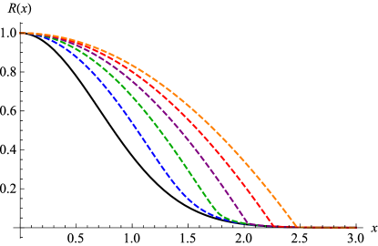
Figure 12: Evolution of Eq. (61): Initial condition at =00\ell=0 (black), followed by =11\ell=1 (blue, dashed), =22\ell=2 (green dashed), =33\ell=3 (purple dashed) , =44\ell=4 (red dashed) and =55\ell=5 (orange, dashed).

This is the celebrated KPZ equation KPZ in the limit of vanishing viscosity. Its solution is known analytically,

(x,)=maxy[(y,0)2(xy)2].𝑥subscript𝑦𝑦02superscript𝑥𝑦2{\cal R}(x,\ell)=\max_{y}\left[{\cal R}(y,0)-\frac{2(x-y)^{2}}{\ell}\right]\ . (62)

As an example, start with (x,0)=ex2𝑥0superscriptesuperscript𝑥2{\cal R}(x,0)=\mathrm{e}^{{-x^{2}}}. The result is shown on figure 12. For large times the maxima are either for y=0𝑦0y=0 or y=x𝑦𝑥y=x, i.e.

(x,){12x2 for 0x20 for x>2.similar-to-or-equals𝑥cases12superscript𝑥2 for 0𝑥20 for 𝑥2{\cal R}(x,\ell)\simeq\left\{\begin{array}[]{cl}\displaystyle 1-\frac{2x^{2}}{\ell}&\mbox{ for }\displaystyle 0\leq x\leq\sqrt{\frac{\ell}{2}}\\ 0&\mbox{ for }\displaystyle x>\sqrt{\frac{\ell}{2}}\rule{0.0pt}{21.52771pt}\end{array}\right.\ . (63)

Note that x2u4similar-tosuperscript𝑥2superscript𝑢4x^{2}\sim u^{4}, yielding the standard ϕ4superscriptitalic-ϕ4\phi^{4}-fixed point in the domain x<l/2𝑥𝑙2x<\sqrt{l/2}.

The rescaled equation reads444Since xu2similar-to𝑥superscript𝑢2x\sim u^{2}, the rescaling term is 2ζxR(x)2𝜁𝑥superscript𝑅𝑥2\zeta xR^{\prime}(x) instead of ζuR(u)𝜁𝑢superscript𝑅𝑢\zeta uR^{\prime}(u).,

mmR(x)=(ε4ζ)R(x)+2ζxR(x)+12R(x)2.𝑚subscript𝑚𝑅𝑥𝜀4𝜁𝑅𝑥2𝜁𝑥superscript𝑅𝑥12superscript𝑅superscript𝑥2-m\partial_{m}R(x)=(\varepsilon-4\zeta)R(x)+2\zeta xR^{\prime}(x)+\frac{1}{2}R^{\prime}(x)^{2}\ . (64)

Since in our solution (63) the function (0,)0{\cal R}(0,\ell) is constant, this implies that ε4ζ=0𝜀4𝜁0\varepsilon-4\zeta=0, thus

ζlargeN=ε4.subscript𝜁large𝑁𝜀4\zeta_{{{\rm large}~{}N}}=\frac{\varepsilon}{4}\ . (65)

There is a shock-front at xc=/2subscript𝑥𝑐2x_{c}=\sqrt{\ell/2}, and the solution R(x,)𝑅𝑥R(x,\ell) grows linearly for x<xc𝑥subscript𝑥𝑐x<x_{c}, i.e. R(x,)(xcx)Θ(xxc)similar-to𝑅𝑥subscript𝑥𝑐𝑥Θ𝑥subscript𝑥𝑐R(x,\ell)\sim(x_{c}-x)\Theta(x\leq x_{c}). This is similar to what we observed in the preceding sections, but with a different exponent. There is no ambiguity about the scaling. That does not mean that there are no solutions for other values of ζ𝜁\zeta: Indeed, we found a family of fixed points with xc=1subscript𝑥𝑐1x_{c}=1, R(xc)=0𝑅subscript𝑥𝑐0R(x_{c})=0, R(xc)=4ζsuperscript𝑅subscript𝑥𝑐4𝜁R^{\prime}(x_{c})=-4\zeta, and series expansion

Refer to caption
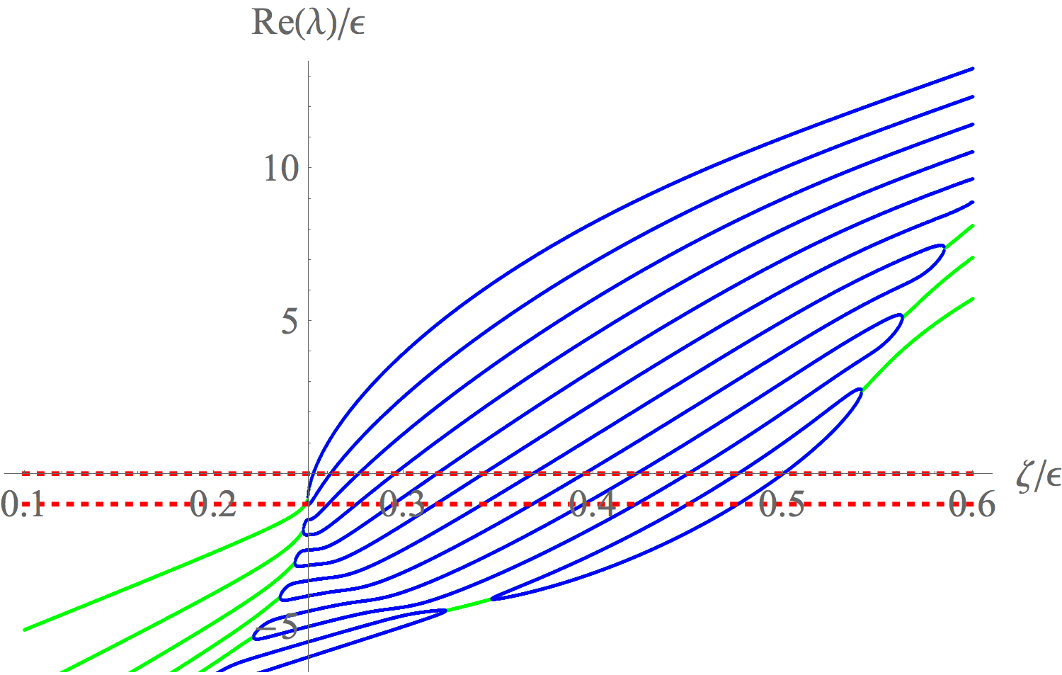
Figure 13: Numerical stability analysis of the fixed-point solutions of Eq. (64), at truncation order 12. All solutions with ζ>ε4𝜁𝜀4\zeta>\frac{\varepsilon}{4} are unstable. Real eigenvalues in blue, complex in green; the latter may be a result of the truncation. Several artefacts due to the truncation can be observed: First, the two exact eigenvalues λ=0𝜆0\lambda=0 and λ=ε𝜆𝜀\lambda=\varepsilon are not correctly reproduced. Second, the largest eigenvalue for ζ=ε4𝜁𝜀4\zeta=\frac{\varepsilon}{4} is not zero, but negative, leading to a small domain of stability for ζ/ε𝜁𝜀\zeta/\varepsilon up to 0.2523; this effect goes away for larger orders, for which however the rounding errors render the plot unreadable. We might only trust the information given for the largest eigenvalue. Finally, the domain for ζ<ε/4𝜁𝜀4\zeta<\varepsilon/4 does not contain a fixed point, as the function R(x)𝑅𝑥R(x) is not defined down to x=0𝑥0x=0. This not-withstanding, we can study stability of the fixed point on a reduced domain for which the Taylor series would still converge; here the plot is instructive in telling us that ζ=ε4𝜁𝜀4\zeta=\frac{\varepsilon}{4} is at the boundary of an island of stability.
R(x)𝑅𝑥\displaystyle R(x) =\displaystyle= 4ζ(x1)+(2ζε)(x1)24𝜁𝑥12𝜁𝜀superscript𝑥12\displaystyle-4{\zeta}(x-1)+(2{\zeta}-\varepsilon)(x-1)^{2} (66)
+16(8ζ+ε2ζ6ε)(x1)3168𝜁superscript𝜀2𝜁6𝜀superscript𝑥13\displaystyle+\frac{1}{6}\left(8{\zeta}+\frac{\varepsilon^{2}}{{\zeta}}-6\varepsilon\right)(x-1)^{3}
+(2ζε)(4ζε)(14ζ5ε)(x1)448ζ22𝜁𝜀4𝜁𝜀14𝜁5𝜀superscript𝑥1448superscript𝜁2\displaystyle+\frac{(2{\zeta}-\varepsilon)(4{\zeta}-\varepsilon)(14{\zeta}-5\varepsilon)(x-1)^{4}}{48{\zeta}^{2}}
+O(x1)5].\displaystyle+O(x-1)^{5}\Big{]}\ .

As for the earlier fixed-point equation (22), the series (66) converges only for

ζlargeNε4.subscript𝜁large𝑁𝜀4\zeta_{{\rm large}~{}N}\geq\frac{\varepsilon}{4}\ . (67)

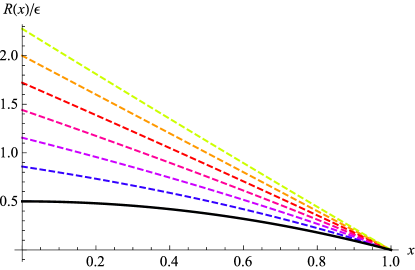
Integrating the fixed-point equation (64) numerically, starting at x1𝑥1x\approx 1, we also find that only when condition (67) is fulfilled, a solution exists from x=1𝑥1x=1 down to x=0𝑥0x=0. These solutions are shown on Fig. 14.
Refer to caption
Figure 14: Fixed points of Eq. (64), for ζ=ε4𝜁𝜀4\zeta=\frac{\varepsilon}{4} (black solid lines), and ζ=0.3ε𝜁0.3𝜀\zeta=0.3\varepsilon, 0.35ε0.6ε0.35𝜀0.6𝜀0.35\varepsilon...0.6\varepsilon (dashed lines, from bottom to top). Only the solution with ζ=ε4𝜁𝜀4\zeta=\frac{\varepsilon}{4} is stable.

All solutions for ζ>ε4𝜁𝜀4\zeta>\frac{\varepsilon}{4} are unstable, and flow to the fixed point with ζ=ε4𝜁𝜀4\zeta=\frac{\varepsilon}{4}, as can bee seen from the explicit solution (62). The latter conclusion is confirmed from a numerical stability analysis, presented on Fig. 13. Its flaws are discussed in the legend of the figure; they may serve as a guideline for the stability analysis presented in section VI, and which conclusions are robust, and which should be discarded.

VIII.2 Disordered elastic manifolds

For disordered elastic manifolds, the central object of interest is the disorder correlator {\cal R}, defined as the disorder average of the potential-potential correlation function (for an introduction see WieseLeDoussal2006 ),

V(x,u)V(x,u)¯=(uu)δd(xx).¯𝑉𝑥𝑢𝑉superscript𝑥superscript𝑢𝑢superscript𝑢superscript𝛿𝑑𝑥superscript𝑥\overline{V(x,u)V(x^{\prime},u^{\prime})}={\cal R}(u-u^{\prime})\delta^{d}(x-x^{\prime})\ . (68)

This correlator {\cal R} has at 1-loop order an RG-equation very similar to Eq. (14) DSFisher1986 ; ChauveLeDoussalWiese2000a ; LeDoussalWieseChauve2003

(u)=12′′(u)2′′(u)′′(0).subscript𝑢12superscript′′superscript𝑢2superscript′′𝑢superscript′′0\partial_{\ell}{\cal R}(u)=\frac{1}{2}{\cal R}^{\prime\prime}(u)^{2}-{\cal R}^{\prime\prime}(u){\cal R}^{\prime\prime}(0)\ . (69)

The presence of the term ′′(u)′′(0)superscript′′𝑢superscript′′0-{\cal R}^{\prime\prime}(u){\cal R}^{\prime\prime}(0) is crucial. For the fixed point the equation to be solved is

mmR(u)𝑚subscript𝑚𝑅𝑢\displaystyle-m\partial_{m}R(u) =\displaystyle= (ε4ζ)R(u)+ζuR(u)𝜀4𝜁𝑅𝑢𝜁𝑢superscript𝑅𝑢\displaystyle(\varepsilon-4\zeta)R(u)+\zeta uR^{\prime}(u) (70)
+12R′′(u)2R′′(u)R′′(0).12superscript𝑅′′superscript𝑢2superscript𝑅′′𝑢superscript𝑅′′0\displaystyle+\frac{1}{2}{R^{\prime\prime}(u)}^{2}-R^{\prime\prime}(u)R^{\prime\prime}(0)\ .

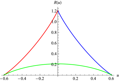
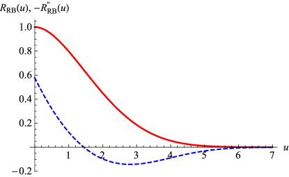
Starting from a Gaussian initial condition for (u)𝑢{\cal R}(u), Eq. (69) flows to a fixed point RRB(u)subscript𝑅RB𝑢R_{{\rm RB}}(u), solution of Eq. (70), and displayed on Fig. 15, with

ζRB0.2082981ε+.similar-to-or-equalssubscript𝜁RB0.2082981𝜀\zeta_{{\rm RB}}\simeq 0.2082981\varepsilon+...\ . (71)

This fixed point is relevant for disordered elastic manifolds subject to random-bond, i.e. short-ranged disorder.

The fixed point has the following properties ChauveLeDoussalWiese2000a ; LeDoussalWieseChauve2003 :

  • (i)

    RRB(0)>0subscript𝑅RB00R_{\rm RB}(0)>0, RRB(0+)=0superscriptsubscript𝑅RBsuperscript00R_{\rm RB}^{\prime}(0^{+})=0, RRB′′(0+)>0superscriptsubscript𝑅RB′′superscript00-R_{\rm RB}^{\prime\prime}(0^{+})>0, RRB′′′(0+)>0superscriptsubscript𝑅RB′′′superscript00R_{\rm RB}^{\prime\prime\prime}(0^{+})>0. Thus RRB(u)subscript𝑅RB𝑢R_{\rm RB}(u) is non-analytic at u=0𝑢0u=0, with a non-analyticity starting at order |u|3superscript𝑢3|u|^{3}.

  • (ii)

    The fixed point has a Gaussian tail, i.e. there exists a constant c𝑐c, s.t. RRB(u)<ecu2subscript𝑅RB𝑢superscripte𝑐superscript𝑢2R_{\rm RB}(u)<\mathrm{e}^{{-cu^{2}}}.

  • (iii)

    The solution is unique, and attractive. The largest two eigenvalues are λ=0𝜆0\lambda=0 and λ=ε𝜆𝜀\lambda=-\varepsilon.

Thus this fixed point has a singularity at u=0𝑢0u=0, and no singularity at finite u=uc<𝑢subscript𝑢cu=u_{\rm c}<\infty. It can be identified and measured in a numerical simulation MiddletonLeDoussalWiese2006 . Let us also mention that for elastic manifolds driven through a disordered environment, a different fixed point is relevant with ζ=ε3𝜁𝜀3\zeta=\frac{\varepsilon}{3}. It can be measured in numerical simulations RossoLeDoussalWiese2006a , and in experiments LeDoussalWieseMoulinetRolley2009 .
Refer to caption
Figure 15: The fixed-point function RRB(u)subscript𝑅RB𝑢R_{{\rm RB}}(u), and its second derivative RRB′′(u)subscriptsuperscript𝑅′′RB𝑢-R^{\prime\prime}_{{\rm RB}}(u) for the fixed-point equation (70). This fixed point is relevant for disordered elastic manifolds with random-bond disorder.

IX Conclusions

In this article, we considered the seemingly familiar setting of scalar field theories; the difference being that contrary to the standard ϕ4superscriptitalic-ϕ4\phi^{4}-potential ours is bounded, and quickly decays to 0. We found that under RG the effective potential develops a cusp at the origin, and a cubic singularity (ucu)3Θ(uuc)similar-toabsentsuperscriptsubscript𝑢c𝑢3Θ𝑢subscript𝑢c\sim(u_{\rm c}-u)^{3}\Theta(u\leq u_{\rm c}) at a shock front ucsubscript𝑢cu_{\rm c} increasing under RG. While there is an infinity of such solutions, our evidence suggests that a specific one is chosen dynamically, when starting from generic smooth initial conditions; this solution has a roughness exponent (dimension of the field) ζ=ε3𝜁𝜀3\zeta=\frac{\varepsilon}{3}.

To put our findings into context, we discussed two similar equations: The first is as above, but at large number of components N𝑁N, which maps onto the KPZ equation. Its analysis is much easier, leading to a roughness exponent ζ=ε4𝜁𝜀4\zeta=\frac{\varepsilon}{4}. The solution also contains a shock-front, with a linear instead of a cubic singularity.

In contrast, for disordered elastic manifolds, a similar flow equation pertains to the renormalization of the disorder correlator. For short-ranged initial conditions, it has a single fixed-point solution with well-defined roughness exponent ζ0.2083εsimilar-to-or-equals𝜁0.2083𝜀\zeta\simeq 0.2083\varepsilon, to which the flow naturally tends. It does not develop a shock singularity at finite uc<subscript𝑢cu_{\rm c}<\infty.

We finally solved a toy model presented in appendix A. Here, singularities appear only after passing via a Legendre transform from the potential 𝒲=ln𝒵𝒲𝒵{\cal W}=\ln{\cal Z} to the action ΓΓ\Gamma. Since at 1-loop order both objects have the same RG-equation, we do not know how to interpret our findings.

Several problems remain a challenge for future research:

  1. (i)

    What is the proper regularization of the RG-equation?

  2. (ii)

    Are there regularizations which lead to distinct critical exponents?

  3. (iii)

    What is the physical interpretation of this new fixed point? Is it relevant for wetting?

  4. (iv)

    What is the phyical interpretation of the cusp, and of the cubic shock front?

  5. (v)

    What is the proper protocol for a simulation?
Refer to caption
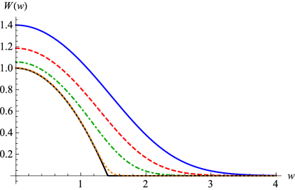
Figure 16: W(w)𝑊𝑤W(w) for the toy model (72) ff. with α=1𝛼1\alpha=-1. From top to bottom: m=0.4𝑚0.4m=0.4 (blue solid), m=0.25𝑚0.25m=0.25 (red dashed), m=0.1𝑚0.1m=0.1 (green, dot-dashed), m=105𝑚superscript105m=10^{-5} (orange, dotted), and the limit of m0𝑚0m\to 0 (black, solid). Both axes are rescaled so that the limit of m0𝑚0m\to 0 exists. (This resealing is a factor of 1/ln(1/m)11𝑚1/\ln(1/m) for the W𝑊W-axes, and a factor of 1/ln(1/m)11𝑚1/\sqrt{\ln(1/m)} for the w𝑤w-axis.)
Acknowledgements.
It is a pleasure to thank Eduoard Brézin for enlightening discussions, and for asking all the right questions. Many thanks go to François David and Andrei Fedorenko for patiently listening and pointing out weak points. I am grateful to Martine Ben Amar, Bernard Derrida and Vincent Hakim for sharing their insights into the analysis of non-linear systems. Financial support from PSL through grant No. ANR-10-IDEX-0001-02-PSL is gratefully acknowledged.

Appendix A Single degree of freedom: A toy model

We consider the following toy model:

V0(u)subscript𝑉0𝑢\displaystyle V_{0}(u) =\displaystyle= eu2superscriptesuperscript𝑢2\displaystyle-\mathrm{e}^{{-u^{2}}} (72)
Vm(u,w)subscript𝑉𝑚𝑢𝑤\displaystyle V_{m}(u,w) =\displaystyle= m22(uw)2.superscript𝑚22superscript𝑢𝑤2\displaystyle\frac{m^{2}}{2}(u-w)^{2}\ . (73)

We define

Wtoy(w):=ln(mα2πdueV0(u)Vm(u,w)).assignsubscript𝑊toy𝑤superscript𝑚𝛼2𝜋superscriptsubscriptdifferential-d𝑢superscriptesubscript𝑉0𝑢subscript𝑉𝑚𝑢𝑤W_{\rm toy}(w):=\ln\!\left(\frac{m^{\alpha}}{\sqrt{2\pi}}\int_{-\infty}^{\infty}\mathrm{d}u\,\mathrm{e}^{-V_{0}(u)-V_{m}(u,w)}\right)\ . (74)

We can rewrite Eq. (74) as

Wtoy(w)=ln(1+mα2πdu(eV0(u)1)eVm(u,w)).subscript𝑊toy𝑤1superscript𝑚𝛼2𝜋superscriptsubscriptdifferential-d𝑢superscriptesubscript𝑉0𝑢1superscriptesubscript𝑉𝑚𝑢𝑤W_{\rm toy}(w)=\ln\!\left(1{+}\frac{m^{\alpha}}{\sqrt{2\pi}}\int_{-\infty}^{\infty}\mathrm{d}u\left(\mathrm{e}^{-V_{0}(u)}{-}1\right)\mathrm{e}^{-V_{m}(u,w)}\right). (75)

Note that we added a factor of mαsuperscript𝑚𝛼m^{\alpha} to mimic for the factor of m2dsuperscript𝑚2𝑑m^{2-d} present in Eq. (6). Formula (75) can more precisely be evaluated numerically, since the integral can be cut off at, say u=±10𝑢plus-or-minus10u=\pm 10. This implies the asymptotic behaviour for small m𝑚m,

Wtoy(w)subscript𝑊toy𝑤\displaystyle W_{\rm toy}(w) similar-to-or-equals\displaystyle\simeq ln(1+mα2πeVm(0,w)(eeu21)du)1superscript𝑚𝛼2𝜋superscriptesubscript𝑉𝑚0𝑤superscriptsubscriptsuperscriptesuperscriptesuperscript𝑢21differential-d𝑢\displaystyle\ln\left(1+\frac{m^{\alpha}}{\sqrt{2\pi}}\mathrm{e}^{-V_{m}(0,w)}\int_{-\infty}^{\infty}(\mathrm{e}^{\mathrm{e}^{-u^{2}}}-1)\,\mathrm{d}u\right) (76)
=\displaystyle= ln(1+1.043mαeVm(0,w))11.043superscript𝑚𝛼superscriptesubscript𝑉𝑚0𝑤\displaystyle\ln\left(1+1.043\,{m^{\alpha}}\,\mathrm{e}^{-V_{m}(0,w)}\right)
\displaystyle\approx 1.043mαeVm(0,w)0.5528m2αe2Vm(0,w)1.043superscript𝑚𝛼superscriptesubscript𝑉𝑚0𝑤0.5528superscript𝑚2𝛼superscripte2subscript𝑉𝑚0𝑤\displaystyle 1.043\,{m^{\alpha}}\,\mathrm{e}^{-V_{m}(0,w)}-0.5528{m^{2\alpha}}\,\mathrm{e}^{-2V_{m}(0,w)}
+.\displaystyle+...\ .

If α𝛼\alpha is positive, the linear term dominates for small m𝑚m, corresponding to the first term in Eq. (6); a linear approximation of the flow equations is appropriate. On the other hand, if α<0𝛼0\alpha<0, the limit is non-trivial, and W𝑊W develops a cusp for m0𝑚0m\to 0. This is presented on figure 16.

Refer to caption
Figure 17: R(u)𝑅𝑢R(u) for the toy model (72) ff. with m=1𝑚1m=1, starting from Eq. (76), and using (78).

On the other hand, for large m𝑚m and α=1𝛼1\alpha=1, we recover the initial condition,

Wtoy(w)V0(w).similar-to-or-equalssubscript𝑊toy𝑤subscript𝑉0𝑤W_{\rm toy}(w)\simeq-V_{0}(w)\ . (77)

We confirmed both limits numerically. Let us now perform the Legendre transform (for m=1𝑚1m=1)

Wtoy(w)+Rtoy(u)Rtoy(0)=uw.subscript𝑊toy𝑤subscript𝑅toy𝑢subscript𝑅toy0𝑢𝑤W_{\rm toy}(w)+R_{\rm toy}(u)-R_{\rm toy}(0)=-uw\ . (78)

We have added a constant R(0)𝑅0R(0), s.t. we can put Rtoy()0subscript𝑅toy0R_{\rm toy}(\infty)\to 0. This transformation is most easily performed numerically, plotting u(w)=Wtoy(w)𝑢𝑤superscriptsubscript𝑊toy𝑤u(w)=-W_{\rm toy}^{\prime}(w) versus Rtoy(u(w))Rtoy(0)=Wtoy(w)wWtoy(w)subscript𝑅toy𝑢𝑤subscript𝑅toy0superscriptsubscript𝑊toy𝑤𝑤subscript𝑊toy𝑤R_{\rm toy}(u(w))-R_{\rm toy}(0)=W_{\rm toy}^{\prime}(w)w-W_{\rm toy}(w). Graphically, this amounts to drawing the tangent to Wtoy(w)subscript𝑊toy𝑤W_{\rm toy}(w), and tracking the intersection of this tangent with the vertical axis. The outcome of this construction is shown on figure 17. It has three branches: Rtoy(u)subscript𝑅toy𝑢R_{\rm toy}(u) starts with a linear slope at u=0𝑢0u=0, resulting from Wtoy(w)subscript𝑊toy𝑤W_{\rm toy}(w) with w>1𝑤1w>1 (blue curve). It terminates at uc>0subscript𝑢c0u_{\rm c}>0, with a term proportional to (uuc)θ(u<uc)𝑢subscript𝑢c𝜃𝑢subscript𝑢c(u-u_{\rm c})\theta(u<u_{\rm c}). The red branch is from w<1𝑤1w<-1. The green branch is the image of 1<w<11𝑤1-1<w<1.

It remains to be clarified what this toy model teaches us about the problem at hand; especially, shall we compare W𝑊W or R𝑅R with the results discussed in the main text?

References

  • (1) K. Wilson and J. Kogut, The renormalization group and the ε𝜀\varepsilon-expansion, Phys. Rep. 12 (1974) 75–200.
  • (2) Edouard Brèzin, Introduction to Statistical Field Theory, Cambridge University Press, 2010.
  • (3) J. Zinn-Justin, Quantum Field Theory and Critical Phenomena, Oxford University Press, Oxford, 1989.
  • (4) J. Cardy, Scaling and Renormalization in Statistical Physics, Cambridge University Press, 1996.
  • (5) D.J. Amit, Field Theory, the Renormalization Group, and Critical Phenomena, World Scientific, Singapore, 2nd edition, 1984.
  • (6) A. Hasenfratz and P. Hasenfratz, Renormalization group study of scalar field theory, Nucl. Phys. B 270 (1986) 687–701.
  • (7) F.J. Wegner and A. Houghton, Renormalization group equation for critical phenomena, Phys. Rev. A 8 (1973) 401–12.
  • (8) J. Polchinski, Renormalization and effective lagrangians, Nucl. Phys. B 231 (1984) 269–95.
  • (9) J. Berges, N. Tetradis and C. Wetterich, Non–perturbative renormalization flow in quantum field theory and statistical physics, Phys. Rep. 363 (2002) 223.
  • (10) E. Brézin, B.I. Halperin and S. Leibler, Critical wetting: the domain of validity of mean field theory, J. Phys. (France) 44 (1983) 775–783.
  • (11) E. Brézin, B.I. Halperin and S. Leibler, Critical wetting in three dimensions, Phys. Rev. Lett. 50 (1983) 1387.
  • (12) D.S. Fisher and D.A. Huse, Wetting transitions: A functional renormalization-group approach, Phys. Rev. B 32 (1985) 247–256.
  • (13) E. Brézin and T. Halpin-Healy, Scaling functions for 3d critical wetting, J. Phys. (France) 48 (1987) 757–761.
  • (14) R. Lipowsky and M.E. Fisher, Scaling regimes and functional renormalization for wetting transitions, Phys. Rev. B 36 (1987) 2126–2241.
  • (15) G. Forgas, R. Lipowsky and T.M. Nieuwenhuizen, The behaviour of interfaces in ordered and disordered systems. Volume 14 of Phase Transitions and Critical Phenomena, pages 136–376, Academic Press London, 1991.
  • (16) F. David, B. Duplantier and E. Guitter, Renormalization of crumpled manifolds, Phys. Rev. Lett. 70 (1993) 2205.
  • (17) F. David, B. Duplantier and E. Guitter, Renormalization theory for interacting crumpled manifolds, Nucl. Phys. B 394 (1993) 555–664.
  • (18) M. Lässig and R. Lipowsky, Critical roughening of interfaces: a new class of renormalizable field theories, Phys. Rev. Lett. 70 (1993) 1131–4.
  • (19) K.J. Wiese, Classification of perturbations for membranes with bending rigidity, Phys. Lett. B 387 (1996) 57–63, cond-mat/9607192.
  • (20) H.A. Pinnow and K.J. Wiese, Interacting crumpled manifolds, J. Phys. A 35 (2002) 1195–1229, cond-mat/0110011.
  • (21) H.A. Pinnow and K.J. Wiese, Interacting crumpled manifolds: Exact results to all orders of perturbation theory, Europhys. Lett. 64 (2003) 371–377, cond-mat/0210007.
  • (22) H.A. Pinnow and K.J. Wiese, Scaling behavior of tethered crumpled manifolds with inner dimension close to d=2: Resumming the perturbation theory, Nucl. Phys. B 711 (2005) 530–564, cond-mat/0403734.
  • (23) M. Kardar and D.R. Nelson, ε𝜀\varepsilon expansions for crumpled manifolds, Phys. Rev. Lett. 58 (1987) 1289 and 2280 E.
  • (24) J.A. Aronovitz and T.C. Lubensky, ε𝜀\varepsilon-expansion for self-avoiding tethered surfaces of fractional dimension, Europhys. Lett. 4 (1987) 395–401.
  • (25) F. David, B. Duplantier and E. Guitter, Renormalization and hyperscaling for self-avoiding manifold models, Phys. Rev. Lett. 72 (1994) 311.
  • (26) F. David, B. Duplantier and E. Guitter, Renormalization theory for the self-avoiding polymerized membranes, cond-mat 9702136 (1997).
  • (27) K.J. Wiese and F. David, Self-avoiding tethered membranes at the tricritical point, Nucl. Phys. B 450 (1995) 495–557, cond-mat/9503126.
  • (28) F. David and K.J. Wiese, Scaling of self-avoiding tethered membranes: 2-loop renormalization group results, Phys. Rev. Lett. 76 (1996) 4564, cond-mat/9602125.
  • (29) K.J. Wiese and F. David, New renormalization group results for scaling of self-avoiding tethered membranes, Nucl. Phys. B 487 (1997) 529–632, cond-mat/9608022.
  • (30) F. David and K.J. Wiese, Large orders for self-avoiding membranes, Nucl. Phys. B 535 (1998) 555–595, cond-mat/9807160.
  • (31) F. David and K.J. Wiese, Instanton calculus for the self-avoiding manifold model, J. Stat. Phys. 120 (2005) 875–1035, cond-mat/0409765.
  • (32) K.J. Wiese, Polymerized membranes, a review. Volume 19 of Phase Transitions and Critical Phenomena, Acadamic Press, London, 1999.
  • (33) P. Le Doussal and K.J. Wiese, Higher correlations, universal distributions and finite size scaling in the field theory of depinning, Phys. Rev. E 68 (2003) 046118, cond-mat/0301465.
  • (34) M. Kardar, G. Parisi and Y.-C. Zhang, Dynamic scaling of growing interfaces, Phys. Rev. Lett. 56 (1986) 889–892.
  • (35) K.J. Wiese and P. Le Doussal, Functional renormalization for disordered systems: Basic recipes and gourmet dishes, Markov Processes Relat. Fields 13 (2007) 777–818, cond-mat/0611346.
  • (36) D.S. Fisher, Interface fluctuations in disordered systems: 5ε5𝜀5-\varepsilon expansion, Phys. Rev. Lett. 56 (1986) 1964–97.
  • (37) P. Chauve, P. Le Doussal and K.J. Wiese, Renormalization of pinned elastic systems: How does it work beyond one loop?, Phys. Rev. Lett. 86 (2001) 1785–1788, cond-mat/0006056.
  • (38) P. Le Doussal, K.J. Wiese and P. Chauve, Functional renormalization group and the field theory of disordered elastic systems, Phys. Rev. E 69 (2004) 026112, cond-mat/0304614.
  • (39) A.A. Middleton, P. Le Doussal and K.J. Wiese, Measuring functional renormalization group fixed-point functions for pinned manifolds, Phys. Rev. Lett. 98 (2007) 155701, cond-mat/0606160.
  • (40) A. Rosso, P. Le Doussal and K.J. Wiese, Numerical calculation of the functional renormalization group fixed-point functions at the depinning transition, Phys. Rev. B 75 (2007) 220201, cond-mat/0610821.
  • (41) P. Le Doussal, K.J. Wiese, S. Moulinet and E. Rolley, Height fluctuations of a contact line: A direct measurement of the renormalized disorder correlator, EPL 87 (2009) 56001, arXiv:0904.4156.