Copyright is held by the International World Wide Web Conference Committee (IW3C2). IW3C2 reserves the right to provide a hyperlink to the author’s site if the Material is used in electronic media.
Social Networks Under Stress
Abstract
Social network research has begun to take advantage of fine-grained communications regarding coordination, decision-making, and knowledge sharing. These studies, however, have not generally analyzed how external events are associated with a social network’s structure and communicative properties. Here, we study how external events are associated with a network’s change in structure and communications. Analyzing a complete dataset of millions of instant messages among the decision-makers in a large hedge fund and their network of outside contacts, we investigate the link between price shocks, network structure, and change in the affect and cognition of decision-makers embedded in the network. When price shocks occur the communication network tends not to display structural changes associated with adaptiveness. Rather, the network “turtles up". It displays a propensity for higher clustering, strong tie interaction, and an intensification of insider vs. outsider communication. Further, we find changes in network structure predict shifts in cognitive and affective processes, execution of new transactions, and local optimality of transactions better than prices, revealing the important predictive relationship between network structure and collective behavior within a social network.
category:
H.2.8 Database Management Database applications—Data miningkeywords:
Social Networks, Organizations, Temporal Dynamics, Collective Behavior.1 Introduction
The emergence of detailed, time-resolved data on large social networks makes it possible to study their structure and dynamics in new ways. Work has identified stable network structures, communities, influentials in networks, information flows, networked teams [1, 2, 3, 4, 5], and the temporal evolution of large social networks [6, 7, 8, 9, 10, 11, 12, 13, 14, 15, 16].
Despite the richness of the available datasets and the computational techniques for analyzing them, work has generally not focused on a crucial feature of dynamic behavior — how changes in the social network’s structure are linked to external shocks. Little research thus far has examined how social networks operate in a reactive capacity, as they respond to such stimuli from their broader environments. By external shocks we mean events that are extreme relative to average events, or unexpected [17]. Such questions are critical to understanding a social network’s capacity to respond to uncertainty when the membership of the network remains essentially fixed. The real-life conditions reflecting these dynamics are varied, including the response of intelligence and law enforcement personnel to emergency situations such as terrorist attacks [18], health professionals responding to outbreaks [19], or organizations facing sudden competitive threats or “normal accidents" [20]. The effect has been to leave a set of basic questions largely unanswered. How does a network respond to external shocks? What can shock-related responses reveal about adaptive collective behavior?
Current frameworks suggest different conjectures for relating social network structure to external risks. Networks could open up structurally, with actors tapping acquaintances who are most likely to provide novel information and diverse perspectives on problem-solving [21]. Experiments show that persons facing threatening job changes, for example, disproportionately turn to their weak ties and reduced their triadic closure [22, 23], broadening their options and access to novel job information [24]. Conversely, external shocks could be associated with networks “turtling up," with actors relying on well-worn sources of information, network insiders, and highly clustered relationships [25, 26] that promote trustworthiness but narrow social cognition [22, 27, 25, 24]. Further, little is known about how individual cognitive and affective reactions aggregate in a network and whether collective reactions are better predicted by knowledge of the shock or structural changes in the network [18].
We address these questions in the context of an organization’s social network [28, 29, 30, 31, 32, 33, 34]. We consider the complete instant-messaging corpus, including content, among the decision-makers of a hedge fund and their outside contacts. The analysis of financial investment behavior is of interest because of its criticality to the economy and society [35, 36, 37, 38, 39, 40].
We focus on a few central questions. First, we study the link between environmental changes — encoded in the movement of the prices of specific stocks at particular points in time — and changes in the network structure, specifically the subgraph consisting of instant messages about these particular stocks during the times in question. For financial services firms, price shocks can represent threatening and stressful external stimuli. Experiments measuring the stress level of traders using conductance technology show that price changes lead to involuntary and significant physiological changes indicative of stress. Shifts in prices cause traders to have increased heart rates and electrodermal responses relative to control conditions [36]. Qualitative observations of traders echo experimental results. In the industry, the VIX, a widely used measure of market price volatility, is referred to as the “Fear Index [41]."
Following sociological theory, one expectation for the association between price shocks and network change is that price shocks are associated with a propensity to activate connections that improve access to novel information and manage risk. In this case, it would be expected that actors in the network would rely relatively more on weak ties, network outsiders, and relationships with low closure. Conversely, shocks may be associated with reflective network structure and behavior [42]. Following this view, expectations are that actors disproportionately favor contacts repeatedly seen in the past, in-group rather than out-group relations, and highly interconnected contacts. In the face of shocks, our analysis supports the conclusion that networks “turtle up" structurally, exhibiting high levels of clustering, out-group communication, and strong ties.
Where our first question explores the link between external factors and network structure, our second main question asks whether these changes to the network structure can yield additional insight into the behavior of the organization — beyond what is provided by the external changes themselves. Specifically, if we seek to predict how the organization will respond to a price change, does knowing properties of the network structure improve the performance of the prediction even if we already have access to the time series of stock prices?
We show that knowledge of the network provides strong improvements in prediction of collective behavior for both individual-level actions and firm-level actions. We evaluate individual-level actions by analyzing the way traders express themselves in the collection of instant messages, using a standard set of linguistic measures. These measures show that when a stock’s price changes significantly (in either the positive or negative direction), the messages associated with that stock display increased emotion and cognitive complexity. While these changes can already be inferred to a limited extent from the price changes alone, we are able to predict their direction and magnitude much more effectively when we incorporate network-level features into the prediction. We find analogous effects in the context of firm-level actions, where we analyze the trading decision employees make for the firm. We introduce a simple measure of local optimality in the trading price and show that network features provide significantly improved performance in predicting whether the firm will perform a locally optimal action. We find a similar pattern when we attempt to predict whether trades that have not been observed for a number of days are suddenly traded.
Taken together, our findings suggest a key role for electronic communication networks in the analysis of external shocks and events affecting an organization: the network displays a consistent set of changes in response to these external events, emphasizing strong ties and clustered structures; and knowledge of the network structure provides significant leverage in predicting the organization’s collective behavior.
2 Data
Our data include the complete instant-messaging communication history among the personnel at a hedge fund, 2010-2011. The data consist of approximately 22 million instant messages (IMs) sent by 8,646 people, of whom 184 are employees of the hedge fund, and the rest are outside contacts. We use the full content of each message and unique person and time of transmission identifiers to analyze the IMs. We know each trade completed at the firm, the stock symbol involved, and date and time of execution. All transactions in our data were executed by the fund’s employees, not algorithms. On average, 559 transactions were performed daily. We merged the above data with public data on daily stock prices. All of our data analysis was consistent with guidelines from the relevant Institutional Review Board
3 Measures
3.1 Network
IMs define a network of information exchange where nodes are communicating actors and IMs between actors define edges. Our primary interest is in the subgraphs of the larger network designated by mentions of particular stocks at particular points in time. For a stock symbol and a day , we define an undirected graph as follows: for each IM between company insiders that mentions stock symbol on day , we include the two participants of the IM as nodes in , and we join them by an edge. We eliminate parallel edges, so that two nodes in will have at most one edge between them. Multiple messages between pairs were examined when relevant. thus consists of all employees who mentioned stock on day , with messages containing on day forming the edges between these people.
| Model 1 | Model 2 | Model 3 | Model 4 | |
| Independent Variables | Nodes | Clustering | Perc. border edges | Strength of ties |
| Stock price change | ||||
| -lag(-1) | ||||
| -lag(-2) | ||||
| VIX | ||||
| 5 Day of week fixed effects | Y | Y | Y | Y |
| Stock fixed effects | Y | Y | Y | Y |
We define an edge to be internal if both nodes are company insiders and border if one node is a company outsider. All IMs include one company employee because communication between company outsiders cannot be recorded. Our definition of uses only internal edges; the analogous construction using both internal and border edges results in a larger graph that contains .
The notation and terminology used in the analysis for graph size and connectivity and quantifications of turtled up or open networks is as follows. Let and be the number of nodes and edges respectively in . We normalize relevant measures in relation to comparable quantities in the data; in particular, for a function that we compute on , we will define to be the ratio of to the average value of for all pairs such that and . This lets us discuss whether is large or small relative to other graphs from previous days with the same number of nodes. We can define the analogous normalization based on the number of edges; we write to denote the ratio of to the average value of for all pairs such that and . Furthermore, since some stocks tend to be more popular in traders’ conversations than others, we normalize the number of nodes. We define as the ratio of to the average values of for all .
| Model 1 | Model 2 | Model 3 | Model 4 | |
| Independent Variables | Nodes | Clustering | Perc. border edges | Strength of ties |
| Stock price change | ||||
| -lag(-1) | ||||
| -lag(-2) | ||||
| VIX | ||||
| 5 Day of week fixed effects | Y | Y | Y | Y |
| Industry fixed effects | Y | Y | Y | Y |
Beyond the number of nodes and edges, a basic quantity is connectivity — whether is connected or whether most nodes belong to few connected components. We write for the fraction of nodes in the largest connected component of , and for the minimum number of components required to account for at least 90% of nodes in .
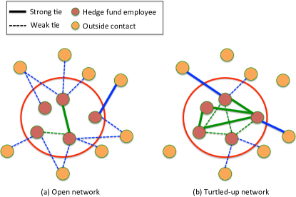
Sociological theory distinguishes “closed" network structures as containing many triangles of relationships (friends of friends link to each other) and a high proportion of strong ties (high-frequency relationships). We are referring to networks with this structure as turtled up networks. Open network structures contain few triangles of relationships and have relatively high numbers of weak ties. Figure 1 illustrates key differences between closed or turtled up networks and open networks.
A measure for capturing triangles of relationship is the clustering coefficient; formally the fraction of pairs of a node’s neighbors that are connected by an edge. We define as the average clustering coefficient over all nodes in . To capture strength of ties we use frequency of communication, which is a relevant measure for the structure of a social network [43]. For each node in , we consider the set of all nodes with whom has participated in any messages on days , and we sort these nodes in descending order by the number of such messages they have participated in . We define as the highest fraction of this sorted list: the fraction of ’s communication partners from the prior day , measured by communication volume these are ’s strongest edges. We quantify whether favors strong or weak ties using the measure , the fraction of edges for which . To the extent that closed and open structures are related to an actor’s reach for information across boundaries [21], we define the openness as the fraction of edges in that are border edges.
3.2 Shocks
To define the extremeness and unexpectedness of price shocks, we defined for each stock and day , and to be the opening and closing prices respectively of stock on day . We define as the proportional change in the price of on day .
Some price changes are disruptive — the price change magnitudes are greater than recent changes, and therefore they can be characterized as unexpected. They intuitively correspond to shocks [17]. We operationalize the notion of a “shock” as follows: a stock-day pair is an -shock if and for . That is, is an -shock if stock ’s price change on day was higher than , and its price change was lower than on the previous three days. We investigate how continuous values of and discrete -shocks relate to the properties of .
4 Findings
4.1 Price Changes and Network Dynamics
We observe a substantial relationship between changes in stock price and changes in network structure. Figure 2 shows how each network feature – clustering, tie strength, and the relative intensity of insider to outsider contacts – changes with . The horizontal axis of each figure shows the percentage price change . When (): the vertical axis indicates the mean measure for networks such that (). When , the vertical axis indicates the mean measure for all networks. Throughout the paper, figures also include 95% confidence intervals. Throughout the paper, figures also include 95% confidence intervals. Aggregating changes in network properties with respect to price changes over all stocks and days, we observe that as price changes increase in intensity, the network exhibits a higher clustering coefficient111We observe consistent results when we measure clustering while controlling for nodes () and edges ().. Price changes are also related to increasing levels of tie strength222In Figure 22(b), we use as the threshold for tie strength. Border edges also drop as a percentage of edges in the face of price changes. Repeating the test with various values of showed that the results are similar regardless of the choice of . These findings reveal that decision-makers in the network tend to turtle up their communication in the face of stress, rather than open up.
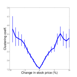
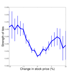
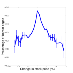
Changes in connectivity are also significant but substantively slight. The fraction of nodes in the largest component increases slightly and the number of components needed to account for 90% of the nodes decreases slightly with price changes. We also find a trend with respect to network size — as the price changes increase, the number of nodes () and edges increases (). These effects are reported for graphs with at least two nodes; all results are consistent if we restrict to graphs containing a larger number of nodes. We note that changes in network structure are symmetric with respect to the direction of the price change, which is curious in nature given that one might expect that price increases and decreases would be associated with different structural changes — an issue we address below when we examine the actual changes in actors’ cognition and affect.
We further examined the results in Figure 2 by disaggregating the analysis on a stock-by-stock and industry-by-industry basis subject to control variables. We run OLS regressions of the form , where is the number of stocks in our data set. For each stock the indicator function is defined as follows as follows:
Including this indicator function as an independent variable measures the association between the change in stock prices, and the network properties on a stock-by-stock basis (i.e., fixed effects model [44]). We included fixed effect variables for day of the week to control communication patterns explained by the day of the week (e.g., earning announcements and quarterly reports typically are made on specific days for specific stocks); a variable measuring the daily market wide volatility using the VIX index; and the lagged values and to control for possible autocorrelation in the time series of network properties.
We run regressions with the described stock level fixed effects and an additional version where we use a fixed effects model at the industry level instead of the stock level. Tables 1 and 2 show the value and significance of each independent variable using fixed effects at the stock and industry level, respectively. The results confirm the analyses presented in Figure 2. Changes in price are associated with increases in network size, clustering, and strength of ties, and decreases in the percentage of outside contacts. A post-test analysis for autocorrelation of the residuals was also run. For each stock , we ran a separate regression of the form . Based on the Durbin-Watson test [45] there was no statistical evidence of positive or negative serial correlation in 99.2% and 99.9% of the stocks, respectively.
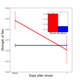
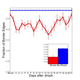
The relationship between unexpected price changes and network structure further substantiate the inference that social networks in the face of uncertainty, as measured here, exhibit a propensity to turtle up. We compare the value of each feature of when is an -shock and when it is not. Further, we measure the number of days a graph feature takes to return to its mean value following a shock. Figure 3 shows the values of network features in graphs on the day of an -shock (, as defined above), and then on subsequent days until the feature approximately returns to its average over all networks. The insets in Figure 3 compare network values on shock and non-shock days. We find that all features are significantly different when there are shocks, and the direction of the differences mirror the previous Figure 2. The same patterns arise when different values of are used. Our analysis of network recovery indicates that most network properties return to their average value one or two days after the shock, suggesting that normalization in relation to these shocks is relatively fast acting.
These results suggest that social networks in the face of stress broadly exhibit features associated with turtling up rather than opening up. Social networks become more intensely interconnected among third parties, rely more on information from strong rather than weak ties, and disproportionately attend to organizational insiders.
4.2 Cognitive and Affective Content
To further understand the behavioral ramifications of network structure in the face of shocks, we explored the links between changes in network structure and the psychology of the actors in the network. If changes in network structure are associated with actual changes in behavior, changes in network structure should predict changes in actors’ cognition and affect. Cognition and affect are important psychological conditions, shaping information processing and decision-making [46, 47, 48].
To infer affect and cognition of the actors in our network, we use the Linguistic Inquiry and Word Count (LIWC) dictionary, which identifies words in the content of communications (i.e., instant messages) that reflect affective and cognitive states333See http://www.liwc.net for more information on LIWC 2007. Affect includes positive emotion, negative emotion, anxiety, anger, and sadness. Cognition includes insight, causation, discrepancy, tentative, certainty, inhibition, inclusive, and exclusive. the LIWC dictionary is well-validated and regularly used [49, 50].
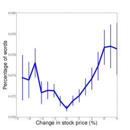
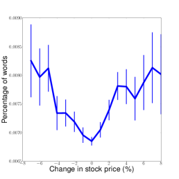
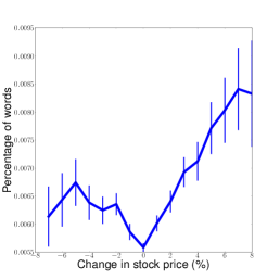
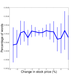
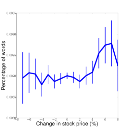
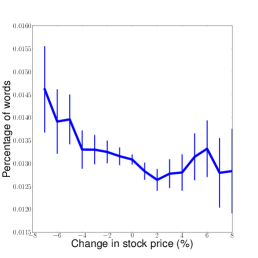
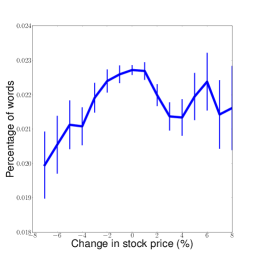
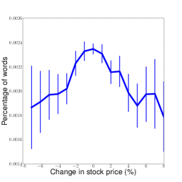
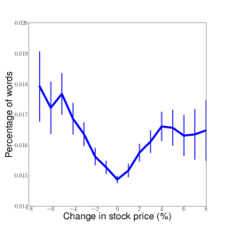
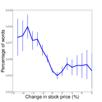
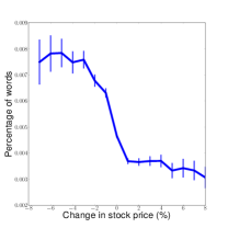
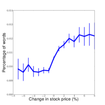
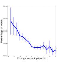
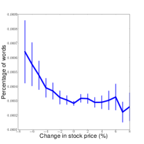
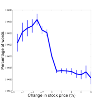
Before incorporating the role of network features, we investigate the relationship between stock prices and IM content by measuring how the usage of LIWC categories varies with changes in the stock prices. In particular, research holds that price changes are stressful for the employees of the firm from a cognitive and emotional perspective [36]. For each instant message among insiders, we computed the percentage of words in each LIWC category. Formally, given a stock-day pair and the IMs that mention on day , we test whether the percentage of LIWC words in the IMs varies with . The x-axis in Figures 4 and 5 show the relative price change . When () and the y- axis indicates the mean percentage of words in each LIWC category in IMs mentioning on day such that (). When , the y- axis indicates the mean value for all IMs.
We find that price changes are associated with expected changes in cognition and affect. Figures 4(f) shows that as price changes intensify, either upward or downward, decision-makers’ communications express higher levels of cognitive processes — presumably because they face greater risk and complexity in their judgments. Figures 4(b-i) show how the different subcategories of cognitive processes change with price. The general trend is that the change in cognitive processes is symmetric in the direction of the price change. This symmetric pattern is consistent with the structural changes in Figure 2.
By contrast, affect expressed during ups and downs in price are asymmetric. Figure 5(a) shows that expressed affect surrounding a stock during its price changes differ depending on whether prices rise or fall. Figures 5(b-f) show the change in the affective subcategories with changes in prices. Words related to positive emotions are used more when stock prices rise while words related to negative emotions, anger, anxiety, and sadness are used more often when stock prices drop. One explanation of this is that while funds can make as much money when stock prices fall as when they rise by selling short, more negative affect is expected when prices drop because falling prices generally sound alarms among retail investors who put their capital in the hands of hedge fund decision-makers and take money out of the market when stock prices fall.
If message content varies with price changes, does network structure further predict the psychology of traders?
To address this question, we formulate the following prediction task. For each stock and each LIWC category , let be the fraction of all IMs containing stock symbol that include a word from category . For each day , let be the fraction of all IMs containing stock symbol on day that include a word from category . We say that the pair conforms to category if — in other words, if words from category are used at a higher rate on day than is typical for stock .
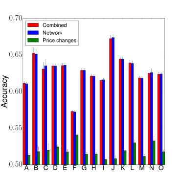
We use binary classifiers to predict whether each pair conforms to each of the cognitive and emotional LIWC categories using the properties of the network and the stock price changes as predictors. We run the prediction test using three feature sets: only network change features (properties of described in section 3.1), only price change features ( and ), and the two sets of features together. Each set of features includes lagged values for 7 days before day . To test the accuracy of the classifiers, we split time into 100-day bins, using each bin as a test set and all the previous bins as training data. We balance the testing and training data by including all positive examples and selecting a random sample of negative examples of the same size as the set of control cases. Table 3 shows the number of cases in each class before being balanced. We use seven binary classifiers: Random Forest, Linear Discriminant Analysis, Quadratic Discriminant Analysis, Naive Bayes, Decision Trees, Support Vector Machines, and Logistic Regression. Choice of classifier does not change the results; logistic regression results are presented.
| Category | Num. Positive | Num. Negative |
| Affective processes | 27229 | 65704 |
| Anger | 3047 | 89886 |
| Anxiety | 1570 | 91363 |
| Causation | 14794 | 78139 |
| Certainty | 13113 | 79820 |
| Cognitive processes | 50088 | 42845 |
| Discrepancy | 19281 | 73652 |
| Exclusive | 27383 | 65550 |
| Inclusive | 36033 | 56900 |
| Inhibition | 7556 | 85377 |
| Insight | 19663 | 73270 |
| Negative emotion | 11478 | 81455 |
| Positive emotions | 23551 | 69382 |
| Sadness | 4531 | 88402 |
| Tentative | 27784 | 65149 |
Figure 6 shows the accuracy of the logistic regression classifier using each of the feature sets for the affective and cognitive categories, and for the positive-emotion, negative-emotion, and insight subcategories. Network properties alone provide significantly better predictions of the psychology of the decision-makers than the price changes alone. Furthermore, the figure indicates that combining the two types of features does not yield a significant improvement over the network features alone. This pattern suggests that network structure is more predictive of a network’s collective affect and cognition than the price shock itself.
4.3 Decision Making Behavior
We now turn to the question of whether the structure of the communication networks provides insight about the trading behavior of the firm. Since trading requires coordination and communication among the employees, it is likely that some of the high level trading decisions of the firm are latent in the structure of the firm’s communication. We look at two important aspects of the decision making process when the firm decides to make a trade – the quality of its trading decision in terms of timing, and the decision to begin trading a stock that has not been traded for a long period of time. Stock prices are crucial in both trading time and in deciding to trade a new stock, hence when we test the predictive value of the networks, we always compare it against the stocks’ price changes. We find that the network structure is indeed predictive of these trading behaviors, above and beyond what is predicted by price changes alone.
4.3.1 Predicting Performance.
We begin by measuring whether the timing of each trade was locally optimal. To measure local optimality of each transaction, we ask whether the firm would have benefited from waiting until the next day to make the transaction. For a stock traded on day we let denote the price of the stock for that transaction. We let and be the maximum and minimum price of stock on day . If a stock was bought on day at price and the maximum price of the following day () was less less than , then the company would have benefited from waiting until the next day to buy stock . Following this reasoning, we label each buy transaction as locally suboptimal if and locally optimal otherwise. Similarly, we label each sell transaction as locally suboptimal if and locally optimal otherwise. We observe that about 20% and 23% of all buy and sell transaction are locally suboptimal.
We expect that the decision process of the firm does not always involve optimizing exactly the day on which to make a transaction. Instead, the firm may focus most of its efforts on other objectives — trying to decide which stocks to trade, how much to trade, or on long term profit as opposed to small gains. To validate our measure of local optimality, we test whether the company’s trades reflect an effort to trade on a locally optimal day by comparing the firm’s real performance with their performance if the trades occurred on a random day.
We create a random set of transactions by taking each transaction in the data set and generating an alternative transaction of the same stock and same number of shares, but on a randomly selected day. The price of the alternative transaction is selected uniformly at random between the minimum and maximum price on the selected day.
The number of locally suboptimal transactions in the random set is 2% higher than in the actual set of transactions. While 2% may not initially appear to be very large, it is easier to assess the size of the difference when we compute the loss in profit that these locally suboptimal transaction generate. For each locally suboptimal transaction , we let the number of shares traded be . The loss generated by this transaction is . The difference in total loss generated by the set of actual transactions and the set of random transaction is about $40 million. This shows that the company performs much better than they would if they traded the same stock and the same number of shares, but on a randomly selected day. This validates our measure; we now test if it is related to features of the networks.
We use our set of classifiers to predict whether transactions are locally optimal using the properties of the network and the stock price changes as predictors. For each transaction of stock on day , we use the features of the graph , the chance in price , and the absolute change in price to predict whether is locally optimal.
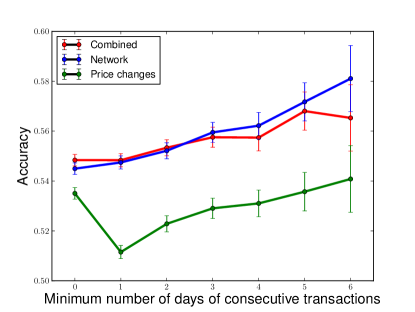
As we did before, we split time into 100 bins, and use each bin as a test set and all the previous bins as training data. We also use a balanced set of positive and negative examples. Since some stocks are traded very often and others are rarely traded, we further split the prediction task into subtasks by the number of consecutive days on which transactions occurred. Letting be the set of transactions that have occurred on at least the previous days, we run the classifiers on each set of transactions for .
Figure 7 shows the accuracy of the Logistic Regression classifier for each set of transactions . The accuracy of the classifiers increases with the number of days of consecutive transitions, suggesting the local optimality of routine transactions is easier to predict than that of unexpected transactions. We also observe that the network features are significantly more predictive than the price changes. Furthermore, combining the network and price change features does not significantly improve the accuracy of the classifier with network features alone. This shows that the local optimality of the firm’s decisions are better aligned with the properties of their communication than the changes in stock prices.
4.3.2 Predicting Sudden Trading
We observed that it’s easier to predict the local optimality of stocks that are traded consecutively. We now turn to a second, more basic question to study the firm-level actions with respect to trading: are we able to predict whether or not a stock is traded on a given day? Our first observation is that many stocks are traded at very high frequencies, and hence the best predictor of a stock being traded on given day is whether it was traded during the previous few days. Given this, we pose the task of predicting new transactions – trades of stocks that have not been traded for a given number of days prior to the transaction being considered.
We let be the set stocks that have not been traded for weeks prior to day . We say that a stock is k-unobserved on day if it is in the set . That is, is -unobserved on day if it has not been traded during the past weeks preceding . Note that a -unobserved stock on day is also -unobserved on day for all . We say that all stocks are -unobserved on all days.
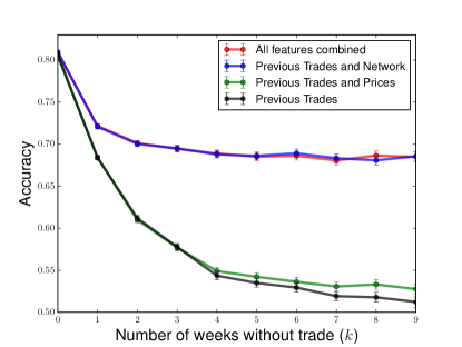
We use our binary classifiers to predict whether stocks that are -unobserved on day will be traded on day . The setup of the prediction task is the same as in the last two sections – we split time into 100 bins and use each bin as a test set and all the previous bins as training data, and we use a balanced set of positive and negative examples. We use network and price change features as we did in previous sections, but in this case we also include features that indicate whether the stock was traded on the 7 days prior to the -week period when the stock was not traded. For example, when we predict if a 1-unobserved stock is traded on day , we know was not traded on days , but we include features that indicate if was traded on days .
Figure 8 shows the accuracy of the classifiers for different values of . When we are predicting whether stocks are traded on day , regardless of whether they have been traded on the previous days. We observe that with no minimum window on the time since the last trade, the 7-day trading history of the stocks provides over 80% accuracy, and adding information about the network or stock prices does not significantly increase the accuracy. However, as increases and we begin predicting trading of stocks that have not been traded for some time, the accuracy of the stocks’ trading history alone drops significantly. When we add the price change features to the trading history features, we do not observe a significant increase in accuracy. However, adding the network features to the trading history features yields a large increase increase in accuracy. For example, for the accuracy of the price change and trading history features is less than 55% and that of the network and trading history features is over %68. Finally, adding price change features to the network and trading history does not significantly increase accuracy. This pattern is consistent with what we found when predicting affective and cognitive content and trading performance.
5 Conclusion
Network science has examined the reaction of networks to internal stresses, particularly nodal loss, but has given considerably less attention to the relationship between external shocks in a network of stable members [51]. Using all the instant messages among stock traders in an investing organization and their outside contacts to define structural, cognitive, and affective properties of their social network, we found that shocks — in the form of extreme price changes — were not associated with conventional adaptive network responses to uncertainty. Rather, the network turtled up. Relationships within the network favored strong ties, high clustering, and company insiders.
Implications of this work relate to networks facing disruptive environments and “normal accidents" [20]. One often cited benefit of networks is that they are more agile than hierarchies and more coordinated than markets in solving collective action problems [34, 52]. While one basis for this benefit has been to show that institutions organized as networks do better than hierarchies in turbulent environments, there has been little work on the actual network dynamics that arise in organizations facing environmental disruptions. Indeed, the 2013 DARPA “robolympics" challenge was instituted to investigate whether machines can work hand in hand with humans to address problems of organizing in the face of “normal accidents" better than humans can on their own. Our case indicated that networks facing shocks turtle up rather than open up. Nevertheless, we find that networks are relatively elastic — turtled up states return to normal states relatively fast. Whether the combination of these changes leads to better or worse performance relative to a set criterion beyond the metrics we investigated, and provided by theory, is a logical research extension and a broad goal for improving knowledge about the scientific functionality and practical management of social networks.
Moreover, we find that the network structure is diagnostic of important patterns of behavior — including the emotional and cognitive content of individual communications, local optimality of transactions, and the sudden execution of new transactions. It is noteworthy that the structure of the networks is more effective at predicting these behavioral patterns than the price changes in the market. This suggests that the network-level changes we observe are not simple offshoots of the underlying price changes, but instead that they carry additional rich information that can be used to analyze the organization’s behavior. Understanding the network’s reaction to shocks can thus be an important factor in understanding the organization more broadly.
The role of the network in this analysis raises a number of further open questions. In particular, while there is a clear relationship between changes in the market and changes in the network, it is interesting to consider what the lower-level mechanisms that produce these effects might be. As we come to better understand the links between shocks, networks, and behavior, we can thus arrive at a clearer picture of networks in the context of their surrounding environments.
6 Acknowledgements
This research was sponsored by the Northwestern University Institute on Complex Systems (NICO), the U. S. Army Research Laboratory and the U. S. Army Research Office under grant number W911NF-09-2-0053, Defense Advanced Research Projects Agency grant BAA-11-64, a Simons Investigator Award, a Google Research Grant, a Facebook Faculty Research Grant, an ARO MURI grant "QUANTA: Quantitative Network-based Models of Adaptive Team Behavior", and NSF grant IIS-0910664. The views and conclusions contained in this document are those of the authors and should not be interpreted as representing the official policies, either expressed or implied, of the Army Research Laboratory or the U.S. government. All our summary statistics and programs are available on request. Northwestern University IRB Approved the Study (#STU00200578). All data were previously collected, accessed from the firm’s archive, anonymized, and involved no manipulation or interaction with subjects. Subjects knew the data were collected and available for research purposes. The firm provided the data under written agreement for research purposes contingent on firm’s identifying characteristics remaining confidential and anonymous.
References
- [1] Newman MEJ. (2003). The structure and function of complex networks. SIAM Review, 45:167–256, 2003.
- [2] Jackson MO. (2008). Social and Economic Networks, Princeton University Press.
- [3] Lazer D. et al (2009), Computational social science, Science 323:721–723.
- [4] Easley DA. and Kleinberg JM. (2010). Networks, Crowds, and Markets, Cambridge University Press.
- [5] Newman MEJ. (2010). Networks: An Introduction, Oxford University Press.
- [6] Barabasi AL., Newman MEJ., and Watts DJ. (2006). The Structure and Dynamics of Networks, Princeton University Press.
- [7] Chakrabarti D. and Faloutsos C. (2012). Graph Mining: Laws, Tools, and Case Studies. Morgan and Claypool.
- [8] Kossinets, G. and Watts, DJ. (2006) Empirical analysis of an evolving social network. Science, 311(5757):88–90.
- [9] Kossinets, G., Kleinberg, J., and Watts, D. (2008) The structure of information pathways in a social communication network. In ACM Proc. KDD 435–443.
- [10] Leskovec, J., Kleinberg, J., and Faloutsos, C. (2007). Graph evolution: Densification and shrinking diameters. ACM Transactions on Knowledge Discovery from Data, 1(1):2.
- [11] Saavedra, S., Hagerty, K., and Uzzi, B. (2011). Synchronicity, instant messaging, and performance among financial traders. Proceedings of the National Academy of Sciences 108(13):5296–5301.
- [12] Qing, K. and Ahn, YY. (2014) Tie strength distribution in scientific collaboration networks. Physical Review E 90(3): 032804.
- [13] Ahn, YY., Han, S., Kwak, H., Moon, S., and Jeong, H. (2007). Analysis of topological characteristics of huge online social networking services. Proceedings of the 16th International Conference on World Wide Web 835–844.
- [14] Peel, L. and Clauset, A. (2015). Detecting change points in the large-scale structure of evolving networks. Proceedings of the 29th International Conference on Artificial Intelligence 2914–2920.
- [15] Weng, L., Ratkiewicz, J., Perra, N., Gon alves, B., Castillo, C., Bonchi, F., Schifanella, R., Menczer, F., and Flammini, A. (2013). The role of information diffusion in the evolution of social networks. In Proceedings of the 19th ACM SIGKDD International Conference on Knowledge discovery and data mining 356–364.
- [16] Viswanath, B., Mislove, A., Cha, M., and Gummadi, KP. (2009). On the evolution of user interaction in Facebook. In Proceedings of the 2nd ACM workshop on Online social networks 37–42.
- [17] Gilbert, CG. (2005) Unbundling the structure of inertia: Resource versus routine rigidity. Academy of Management Journal 48(5):741–763.
- [18] Butts, C. T., Petrescu-Prahova, M., and Remy Cross, B. (2007). Responder communication networks in the World Trade Center disaster: Implications for modeling of communication within emergency settings. Mathematical Sociology, 31(2):121–147.
- [19] Dutta, S., and Rao, H. (2015). Infectious diseases, contamination rumors and ethnic violence: Regimental mutinies in the Bengal Native Army in 1857 India. Organizational Behavior and Human Decision Processes, 129:36–47.
- [20] Perrow, C. (2011). Normal accidents: Living with high risk technologies. Princeton University Press.
- [21] Burt, RS. (1992) Structural Holes: The Social Structure of Competition. Harvard University Press.
- [22] Menon, T., and Smith, EB. (2014) Identities in flux: Cognitive network activation in times of change. Social science research 45:117–130.
- [23] Smith, EB., Menon, T., and Thompson, L. (2012) Status differences in the cognitive activation of social networks. Organization Science 23(1):67–82.
- [24] Granovetter, MS. (1973). The strength of weak ties. American journal of sociology 1360–1380.
- [25] Coleman, JS. (1988). Social capital in the creation of human capital. American Journal of Sociology, 94:95–120.
- [26] Granovetter, MS. (1985). Economic action, social structure, and embeddedness. American Journal of Sociology 91:481–510.
- [27] Ellis, AP. (2006) System breakdown: The role of mental models and transactive memory in the relationship between acute stress and team performance. Academy of Management Journal 49(3):576–589.
- [28] Adamic, L. and Adar, E. (2005) How to search a social network. Social Networks 27(3):187–203.
- [29] Brass, DJ., Galaskiewicz, J., Greve, HR., and Tsai, W. (2004) Taking stock of networks and organizations: A multilevel perspective. Academy of management journal 47(6):795–817.
- [30] Diesner, J., Frantz, T-L., and Carley, K-M. (2005) Communication networks from the Enron email corpus “it’s always about the people. Enron is no different". Computational & Mathematical Organization Theory 11(3):201–228.
- [31] Dodds, PS., Watts, DJ., and Sabel, CF. (2003) Information exchange and the robustness of organizational networks. Proceedings of the National Academy of Sciences 100(21):12516–12521.
- [32] Kilduff M. and Shipilov AV. (Eds) (2011). Organizational Network Research. SAGE Publications.
- [33] Klimt, B. and Yang, Y. (2004) The enron corpus: A new dataset for email classification research. Machine learning: ECML. 217–226.
- [34] Uzzi B. (1996). The Sources and Consequences of Embeddedness for the Economic Performance of Organizations: The Network Effect. Am. Sociol. Rev. 61:674–698
- [35] Fenton-O’Creevy, M., Soane, E., Nicholson, N., Willman, P. (2011). Thinking, feeling and deciding: the influence of emotions on the decision making and performance of traders. Journal of Organizational Behavior 32(8) 1044–1061.
- [36] Lo, AW., Repin, DW. (2002). The psychophysiology of real-time financial risk processing. Journal of cognitive neuroscience 14:323–339.
- [37] Preis, T., Moat, HS., Stanley, HE. (2013). Quantifying Trading Behavior in Financial Markets Using Google Trends. Nature Scientific Report 3:1684.
- [38] Saavedra, S., Malmgren, RD., Switanek, N., Uzzi, B. (2013). Foraging under Conditions of Short-term Exploitative Competition: The Case of Stock Traders. Proceedings of the Royal Society of London B: Biological Sciences 1471–2954.
- [39] Gell-Mann, M., Lloyd S. (1996). Information measures, Effective Complexity, and Total Information. Complexity 2(1):44–52.
- [40] Fama E., (1970). Efficient Capital Markets: A Review of Theory and Empirical Work. The journal of Finance 25(2):383–417.
- [41] Whaley, R. E. (2000). The investor fear gauge. The Journal of Portfolio Management 26(3) 12–17.
- [42] Staw BM., Sandelands LE., Dutton JE. (1981) Threat-rigidity effects in organizational behavior: A multilevel analysis. Administrative Science Quarterly 26:501–524.
- [43] De Choudhury, M., Mason, W. A., Hofman, J. M., and Watts, D. J. (2010). Inferring relevant social networks from interpersonal communication. In Proceedings of the 19th International Conference on World Wide Web 301-310.
- [44] Bhargava, A., Franzini, L., and Narendranathan, W. (1982). Serial correlation and the fixed effects model. The Review of Economic Studies 49(4): 533–549.
- [45] Durbin, J., and Watson, GS. (1950). Testing for serial correlation in least squares regression. I. Biometrika 37(3-4): 409–428.
- [46] Kahneman, D. (2011). Thinking, fast and slow. Macmillan.
- [47] Tetlock, PC. (2007). Giving content to investor sentiment: The role of media in the stock market. The Journal of Finance 62(3):1139–1168.
- [48] Agarwal, S., Duchin, R., and Sosyura, D. (2012). In the Mood for a Loan: The Causal Effect of Sentiment on Credit Origination. Available at SSRN 2141030.
- [49] Kramer, AD., Guillory, JE., Hancock, JT. (2014) Experimental Evidence of Massive-scale Emotional Contagion Through Social Networks. Proceedings of the National Academy of Sciences 111(24):8788–8790.
- [50] Coviello, L., Sohn, Y., Kramer, AD., Marlow, C., Franceschetti, M., Christakis, NA., Fowler, JH. (2014). Detecting Emotional Contagion in Massive Social Networks. PLoS ONE 9(3):e90315.
- [51] Saavedra, S., Reed-Tsochas, F., Uzzi, B. (2008). Asymmetric disassembly and robustness in declining networks. Proceedings of the National Academy of Sciences 105(43): 16466–16471.
- [52] Powell, W. (2003). Neither market nor hierarchy. it The sociology of organizations: classic, contemporary, and critical readings 315:104–117.