Redeker and Wunderlich

Portfolio optimization under dynamic risk constraints: continuous vs.discrete time trading

Imke Redeker Mathematical Institute, Brandenburg University of Technology Cottbus - Senftenberg, Postbox 101344, 03013 Cottbus, Germany Ralf Wunderlich Mathematical Institute, Brandenburg University of Technology Cottbus - Senftenberg, Postbox 101344, 03013 Cottbus, Germany
Abstract

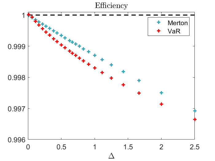
We consider an investor facing a classical portfolio problem of optimal investment in a log-Brownian stock and a fixed-interest bond, but constrained to choose portfolio and consumption strategies that reduce a dynamic shortfall risk measure. For continuous- and discrete-time financial markets we investigate the loss in expected utility of intermediate consumption and terminal wealth caused by imposing a dynamic risk constraint. We derive the dynamic programming equations for the resulting stochastic optimal control problems and solve them numerically. Our numerical results indicate that the loss of portfolio performance is not too large while the risk is notably reduced. We then investigate time discretization effects and find that the loss of portfolio performance resulting from imposing a risk constraint is typically bigger than the loss resulting from infrequent trading.

1 Introduction

sec:Introduction In a classical consumption-investment problem, an investor endowed with an initial capital consumes a certain amount of the capital and invests the remaining wealth into the financial market. The latter usually consists of one risk-free security and several risky ones. Given a fixed investment horizon, the investor's objective is to find an ``optimal'' consumption-investment strategy in order to maximize the expected utility of wealth at the terminal trading time and of intermediate consumption. This optimization problem is known in the literature as the Merton problem.

After the recent failure of large financial institutions, risk management has received a great deal of attention by traders and regulators in the past few years. Financial institutions have established internal departments that are in charge of risk assessments, and regulatory institutions started to set restrictions to limit the risk exposure of financial institutions. Various risk measures like Value at Risk (VaR) or some tail-expectation-based risk measures like Tail Conditional Expectation (TCE) or Expected Loss (EL) have been applied recently to quantify and control the risk of a portfolio. Usually the risk constraint is static, i.e., it has to hold at the terminal trading time only. In the seminal paper by Basak and Shapiro [6] the authors compute the VaR of the terminal wealth to control the risk exposure. Their findings indicate that VaR limits, when applied in a static manner, may actually increase risk. This encouraged researchers to consider a risk measure that is based on the risk neutral expectation of loss - the Limited Expected Loss (LEL). The work of [6] is extended by Gabih et al. [10] to cover the case of bounded Expected Loss.

Motivated by the Basel Committee proposals, it is a common practice in the financial industry to compute and re-evaluate risk constraints frequently using a time window (e.g. some days or weeks) over which the trading strategies are assumed to be held constant, cf. Jorion [14]. Therefore Cuoco et al. [7] apply a risk constraint dynamically to control the risk exposure. The authors found that VaR and TCE constraints, when applied in a dynamic fashion, reduce the investment in the risky asset. PutschΓΆgl and Sass [21] study the maximization of expected utility of terminal wealth under dynamic risk constraints in a complete market model with partial information on the drift by using the martingale method. The problem of intertemporal consumption subject to a dynamic VaR constraint is studied by Yiu [24]. Pirvu [20] and Leippold et al. [16] study an optimal consumption-investment problem with a dynamic VaR constraint imposed on the strategy. Akume [1] and Akume et al. [2] consider a similar problem with a dynamic TCE constraint instead of a VaR. Their results indicate that imposing a dynamic risk constraint is a suitable method to reduce the risk of portfolios. For recent work on portfolio optimization under dynamic risk constraints we refer to Moreno-Bromberg et al. [17]. The authors study an optimal investment problem for a general class of risk measures and the optimal trading strategy is characterized by a quadratic backward stochastic differential equation.

For the purpose of dynamic risk measurement, the usual assumption for a tractable way of calculating risk measures is that the investment and consumption strategies are kept unchanged over a given time horizon. In the classical consumption-investment problem, this assumption is typically not fulfilled. An investor who follows the optimal strategy is continuously adjusting the asset holdings and the consumption rate. Thus, the risk of a portfolio is only approximately calculated.

Since continuous-time trading is impossible in practice and investors want to avoid transaction costs due to excessive trading we also consider a more realistic scenario where investors are only allowed to change the asset holdings and consumption rate at discrete points in time. In Rogers [22] and BΓ€uerle et al. [4] such a discrete-time investor is called a relaxed investor. It is shown that the losses due to discretization are surprisingly small. An advantage of the discrete-time trading is that dynamic risk measures can be computed directly without requiring constant strategies.

In this paper, we start with considering a continuous-time investor facing a classical consumption-investment problem, but constrained to choose investment and consumption strategies that reduce a corresponding shortfall risk. The investor's aim is to maximize the expected utility of the intermediate consumption and wealth at a terminal trading time T>0𝑇0T>0. The portfolio risk over short time intervals is measured in terms of VaR, TCE and EL. The risk measure is dynamically re-evaluated using available conditioning information and imposed on the strategy as a risk constraint. We apply dynamic programming techniques and combine the resulting Hamilton-Jacobi-Bellman equation with the method of Lagrange multipliers to derive optimal strategies under this constraint. An approximate solution to the constrained portfolio problem is obtained by using a policy improvement algorithm. One advantage of our method compared to [17] is that the consumption of wealth can easily be included.

Then, we consider a discrete-time investor who only changes portfolio and consumption choices at time points that are multiples of Ξ”>0Ξ”0\Delta>0. Within the framework of a discrete-time investment, we consider a discretized standard Black-Scholes market with one risk-free and several risky assets. A discrete-time investor is, like a continuous-time investor, constrained to limit the risk exposure. The optimization problem is solved by using the theory of Markov Decision Problems leading to a backward recursion algorithm.

Our numerical results indicate that the cost of the risk constraint in terms of the expected utility of intermediate consumption and terminal wealth is not too large while the risk can be controlled and considerably reduced. The consideration of both, discrete-time and continuous-time trading, allows us to perform numerical experiments for studying the losses due to time-discretization. Similar to Rogers [22] who investigates the Merton problem, we find that for the portfolio problem under dynamic risk constraints the effects of time-discretization are also of small magnitude.

The paper is organized as follows. In Section LABEL:sec2 we consider the continuous-time optimization problem. First, we describe the financial market model and introduce dynamic risk constraints afterwards. Then, we investigate the optimization problem under dynamic risk constraints. In Section LABEL:sec3, we consider the discrete-time optimization problem. The financial market of Section LABEL:sec2 is discretized and the resulting dynamic risk constraints are described. We subsequently study the discrete-time optimization problem under dynamic risk constraints. Section LABEL:sec4 provides some numerical results of the continuous-time and discrete-time optimization problem and both are compared. The Appendix contains proofs omitted from the main text.

2 Continuous-time optimization

sec2

2.1 Model

We consider a continuous-time stochastic financial market with finite trading horizon 0<T<∞0𝑇0<T<\infty. The possible actions of an investor who is endowed with an initial capital x0>0subscriptπ‘₯00x_{0}>0 are to invest in the financial market and/or to consume (parts of) the wealth. The investment opportunities are represented by one risk-free and d𝑑d risky securities. The price of the risk-free security at time t𝑑t is denoted by St0superscriptsubscript𝑆𝑑0S_{t}^{0} and the d𝑑d-dimensional price process of the risky securities is denoted by 𝑺=(𝑺t)t∈[0,T]𝑺subscriptsubscript𝑺𝑑𝑑0𝑇\boldsymbol{S}=(\boldsymbol{S}_{t})_{t\in[0,T]}. Uncertainty is modeled by a filtered probability space (Ξ©,β„±,𝔽,P)Ωℱ𝔽𝑃(\Omega,{\cal F},{\mathbb{F}},{P}), where 𝔽=(β„±t)t∈[0,T]𝔽subscriptsubscriptℱ𝑑𝑑0𝑇{\mathbb{F}}=({\cal F}_{t})_{t\in[0,T]} is the natural filtration generated by an mπ‘šm-dimensional Brownian motion 𝑾=(𝑾t)t∈[0,T]𝑾subscriptsubscript𝑾𝑑𝑑0𝑇\boldsymbol{W}=(\boldsymbol{W}_{t})_{t\in[0,T]}, mβ‰₯dπ‘šπ‘‘m\geq d, augmented by all the P𝑃{P}-null sets of ΩΩ\Omega.
The risk-free security (the ``bond'') behaves like a bank account earning a continuously compounded interest rate rβ‰₯0π‘Ÿ0r\geq 0, i.e., its price is given by

St0=er​t.superscriptsubscript𝑆𝑑0superscriptπ‘’π‘Ÿπ‘‘\displaystyle S_{t}^{0}=e^{rt}.

The remaining d𝑑d securities (the ``stocks'') are risky and evolve according to the following stochastic differential equations

d​Stidsuperscriptsubscript𝑆𝑑𝑖\displaystyle{\text{d}}S_{t}^{i} =Sti​(ΞΌi​d​t+βˆ‘j=1mΟƒi​j​d​Wtj),i=1,…,d,formulae-sequenceabsentsuperscriptsubscript𝑆𝑑𝑖superscriptπœ‡π‘–d𝑑superscriptsubscript𝑗1π‘šsuperscriptπœŽπ‘–π‘—dsuperscriptsubscriptπ‘Šπ‘‘π‘—π‘–1…𝑑\displaystyle=S_{t}^{i}\Big{(}\mu^{i}{\text{d}}t+\sum_{j=1}^{m}\sigma^{ij}{\text{d}}W_{t}^{j}\Big{)},\quad i=1,\ldots,d,
S0isuperscriptsubscript𝑆0𝑖\displaystyle S_{0}^{i} =si,absentsuperscript𝑠𝑖\displaystyle=s^{i},

where 𝝁=(ΞΌi)i=1,…,dβˆˆβ„d𝝁subscriptsuperscriptπœ‡π‘–π‘–1…𝑑superscriptℝ𝑑\boldsymbol{\mu}=(\mu^{i})_{i=1,\ldots,d}\in{\mathbb{R}}^{d} is the mean rate of return and 𝝈=(Οƒi​j)i=1,…,dj=1,…,mβˆˆβ„dΓ—m𝝈subscriptsuperscriptsuperscriptπœŽπ‘–π‘—π‘—1β€¦π‘šπ‘–1…𝑑superscriptβ„π‘‘π‘š\boldsymbol{\sigma}=(\sigma^{ij})^{j=1,\ldots,m}_{i=1,\ldots,d}\in{\mathbb{R}}^{d\times m} the matrix-valued volatility which is assumed to consist of linearly independent rows. Thus, we work on a standard Black-Scholes-Merton model. The bond and the stocks can be traded continuously and we allow to sell the stock and the bond short. An investment strategy 𝝅=(𝝅t)t∈[0,T]𝝅subscriptsubscript𝝅𝑑𝑑0𝑇\boldsymbol{\pi}=(\boldsymbol{\pi}_{t})_{t\in[0,T]} is an 𝔽𝔽{\mathbb{F}}-adapted, real-valued, d𝑑d-dimensional stochastic process satisfying

𝔼​[∫0Tβˆ₯𝝅tβˆ₯2​d​t]<∞,𝔼delimited-[]superscriptsubscript0𝑇superscriptdelimited-βˆ₯βˆ₯subscript𝝅𝑑2d𝑑\displaystyle{\mathbb{E}}\Big{[}\int\nolimits_{0}^{T}\lVert\boldsymbol{\pi}_{t}\rVert^{2}{\text{d}}t\Big{]}<\infty,

where βˆ₯β‹…βˆ₯delimited-βˆ₯βˆ₯β‹…\lVert\cdot\rVert denotes the standard Euclidean norm in ℝdsuperscriptℝ𝑑{\mathbb{R}}^{d}. The d𝑑d coordinates of 𝝅tsubscript𝝅𝑑\boldsymbol{\pi}_{t} represent the proportions of the current wealth invested in each of the d𝑑d stocks at time t𝑑t.

A negative proportion Ο€tisuperscriptsubscriptπœ‹π‘‘π‘–\pi_{t}^{i} corresponds to selling stock i𝑖i short. The proportion of wealth invested in the bond at time t𝑑t is given by 1βˆ’βˆ‘i=1dΟ€ti1superscriptsubscript𝑖1𝑑superscriptsubscriptπœ‹π‘‘π‘–1-\sum_{i=1}^{d}\pi_{t}^{i}. If this quantity is negative we sell the bond short, i.e., we are borrowing (at interest rate rπ‘Ÿr). The investor is also allowed to withdraw funds for consumption. The consumption rate process (for brevity: consumption process) is denoted by C=(Ct)t∈[0,T]𝐢subscriptsubscript𝐢𝑑𝑑0𝑇C=(C_{t})_{t\in[0,T]}. It is an adapted, [0,∞)0[0,\infty)-valued stochastic process satisfying

𝔼​[∫0TCt​d​t]<∞.𝔼delimited-[]superscriptsubscript0𝑇subscript𝐢𝑑d𝑑\displaystyle{\mathbb{E}}\Big{[}\int\nolimits_{0}^{T}C_{t}\,{\text{d}}t\Big{]}<\infty.

Given an investment and consumption strategy the associated wealth process is well defined and satisfies the stochastic differential equation

e​q:w​e​a​l​t​h​d​Xt=Xt​(1βˆ’βˆ‘i=1dΟ€ti)​r​d​t+Xt​𝝅t′​𝝁​d​tβˆ’Ct​d​t+Xt​𝝅tβ€²β€‹πˆβ€‹d​𝑾t=Xt​(r+𝝅t′​(πβˆ’πŸβ€‹r)βˆ’ct)​d​t+Xt​𝝅tβ€²β€‹πˆβ€‹d​𝑾t,:π‘’π‘žπ‘€π‘’π‘Žπ‘™π‘‘β„Ždsubscript𝑋𝑑subscript𝑋𝑑1superscriptsubscript𝑖1𝑑superscriptsubscriptπœ‹π‘‘π‘–π‘Ÿd𝑑subscript𝑋𝑑superscriptsubscript𝝅𝑑′𝝁d𝑑subscript𝐢𝑑d𝑑subscript𝑋𝑑superscriptsubscriptπ…π‘‘β€²πˆdsubscript𝑾𝑑subscriptπ‘‹π‘‘π‘Ÿsuperscriptsubscript𝝅𝑑′𝝁1π‘Ÿsubscript𝑐𝑑d𝑑subscript𝑋𝑑superscriptsubscriptπ…π‘‘β€²πˆdsubscript𝑾𝑑\displaystyle\begin{split}{eq:wealth}{\text{d}}X_{t}&=X_{t}\Big{(}1-\sum_{i=1}^{d}\pi_{t}^{i}\Big{)}r\,{\text{d}}t+X_{t}\boldsymbol{\pi}_{t}^{\prime}\boldsymbol{\mu}\,{\text{d}}t-C_{t}{\text{d}}t+X_{t}\boldsymbol{\pi}_{t}^{\prime}\boldsymbol{\sigma}{\text{d}}\boldsymbol{W}_{t}\\ &=X_{t}\left(r+\boldsymbol{\pi}_{t}^{\prime}(\boldsymbol{\mu}-{\mathbf{1}}r)-c_{t}\right){\text{d}}t+X_{t}\boldsymbol{\pi}_{t}^{\prime}\boldsymbol{\sigma}{\text{d}}\boldsymbol{W}_{t},\end{split} (1)

where 𝝅tβ€²superscriptsubscript𝝅𝑑′\boldsymbol{\pi}_{t}^{\prime} denotes the transpose of 𝝅tsubscript𝝅𝑑\boldsymbol{\pi}_{t}, 𝟏:=(1,…,1)β€²assign1superscript1…1β€²\mathbf{1}:=(1,\ldots,1)^{\prime} is the d𝑑d-dimensional vector with unit components and ct=Ct/Xtsubscript𝑐𝑑subscript𝐢𝑑subscript𝑋𝑑c_{t}=C_{t}/X_{t} is the consumption rate relative to the wealth. Together with the initial condition X0=x0subscript𝑋0subscriptπ‘₯0X_{0}=x_{0}, the wealth equation (LABEL:eq:wealth) admits a unique strong solution given by

e​q:w​e​a​l​t​hs​o​l​Xt=x0​exp⁑{∫0t(r+𝝅s′​(πβˆ’πŸβ€‹r)βˆ’csβˆ’12​βˆ₯𝝅sβ€²β€‹πˆβˆ₯2)​d​s+∫0t𝝅sβ€²β€‹πˆβ€‹d​𝑾s}.:π‘’π‘žπ‘€π‘’π‘Žπ‘™π‘‘subscriptβ„Žπ‘ π‘œπ‘™subscript𝑋𝑑subscriptπ‘₯0superscriptsubscript0π‘‘π‘Ÿsuperscriptsubscript𝝅𝑠′𝝁1π‘Ÿsubscript𝑐𝑠12superscriptdelimited-βˆ₯βˆ₯superscriptsubscriptπ…π‘ β€²πˆ2d𝑠superscriptsubscript0𝑑superscriptsubscriptπ…π‘ β€²πˆdsubscript𝑾𝑠\displaystyle{eq:wealth_{s}ol}X_{t}=x_{0}\exp\bigg{\{}\int_{0}^{t}\Big{(}r+\boldsymbol{\pi}_{s}^{\prime}(\boldsymbol{\mu}-{\mathbf{1}}r)-c_{s}-\frac{1}{2}\lVert\boldsymbol{\pi}_{s}^{\prime}\boldsymbol{\sigma}\rVert^{2}\Big{)}{\text{d}}s+\int_{0}^{t}\boldsymbol{\pi}_{s}^{\prime}\boldsymbol{\sigma}{\text{d}}\boldsymbol{W}_{s}\bigg{\}}. (2)

Note that (LABEL:eq:wealth_sol) implies

e​q:w​e​a​l​t​hs​o​l​1​Xt+Ξ”=Xt​exp⁑{∫tt+Ξ”(r+𝝅s′​(πβˆ’πŸβ€‹r)βˆ’csβˆ’12​βˆ₯𝝅sβ€²β€‹πˆβˆ₯2)​d​s+∫tt+Δ𝝅sβ€²β€‹πˆβ€‹d​𝑾s}:π‘’π‘žπ‘€π‘’π‘Žπ‘™π‘‘subscriptβ„Žπ‘ π‘œπ‘™1subscript𝑋𝑑Δsubscript𝑋𝑑superscriptsubscriptπ‘‘π‘‘Ξ”π‘Ÿsuperscriptsubscript𝝅𝑠′𝝁1π‘Ÿsubscript𝑐𝑠12superscriptdelimited-βˆ₯βˆ₯superscriptsubscriptπ…π‘ β€²πˆ2d𝑠superscriptsubscript𝑑𝑑Δsuperscriptsubscriptπ…π‘ β€²πˆdsubscript𝑾𝑠\displaystyle{eq:wealth_{s}ol1}X_{t+\Delta}=X_{t}\exp\bigg{\{}\!\!\int_{t}^{t+\Delta}\!\!\big{(}r+\boldsymbol{\pi}_{s}^{\prime}(\boldsymbol{\mu}-{\mathbf{1}}r)\!-c_{s}\!-\frac{1}{2}\lVert\boldsymbol{\pi}_{s}^{\prime}\boldsymbol{\sigma}\rVert^{2}\big{)}{\text{d}}s+\!\!\int_{t}^{t+\Delta}\!\boldsymbol{\pi}_{s}^{\prime}\boldsymbol{\sigma}{\text{d}}\boldsymbol{W}_{s}\!\bigg{\}} (3)

for any Ξ”>0Ξ”0\Delta>0. A pair (𝝅t,ct)t∈[0,T]subscriptsubscript𝝅𝑑subscript𝑐𝑑𝑑0𝑇(\boldsymbol{\pi}_{t},c_{t})_{t\in[0,T]} is called a portfolio-proportion process. We only consider those portfolio-proportion processes 𝒖=(𝝅,c)𝒖𝝅𝑐\boldsymbol{u}=(\boldsymbol{\pi},c) which achieve a positive wealth over the whole trading period [0,T]0𝑇[0,T] and which are of Markov type, i.e., 𝒖t=u~​(t,Xt)subscript𝒖𝑑~𝑒𝑑subscript𝑋𝑑\boldsymbol{u}_{t}=\widetilde{u}(t,X_{t}) for all t∈[0,T]𝑑0𝑇t\in[0,T] and some measurable function u~:[0,T]×ℝ+→𝒦:~𝑒→0𝑇subscriptℝ𝒦\widetilde{u}\colon[0,T]\times{\mathbb{R}}_{+}\to{\cal K} where 𝒦:=ℝdΓ—[0,∞)assign𝒦superscriptℝ𝑑0{\cal K}:={\mathbb{R}}^{d}\times[0,\infty). Such strategies are called admissible and the set of admissible strategies is denoted by π’œ0subscriptπ’œ0{\cal A}_{0}, thus

π’œ0:={\displaystyle{\cal A}_{0}:=\Big{\{} (𝒖t)t∈[0,T]|𝒖​ is ​𝔽​-adapted,𝒖t=(𝝅t,ct)βˆˆπ’¦,𝒖t=u~​(t,Xt),formulae-sequenceconditionalsubscriptsubscript𝒖𝑑𝑑0𝑇𝒖 is 𝔽-adaptedsubscript𝒖𝑑subscript𝝅𝑑subscript𝑐𝑑𝒦subscript𝒖𝑑~𝑒𝑑subscript𝑋𝑑\displaystyle(\boldsymbol{u}_{t})_{t\in[0,T]}\,\Big{|}\,\boldsymbol{u}\text{ is }{\mathbb{F}}\text{-adapted},\boldsymbol{u}_{t}=(\boldsymbol{\pi}_{t},c_{t})\in{\cal K},\boldsymbol{u}_{t}=\widetilde{u}(t,X_{t}),
Xt>0Β for allΒ t∈[0,T]Β and 𝔼[∫0T(βˆ₯𝝅tβˆ₯2+ct)dt]<∞}.\displaystyle X_{t}>0\text{ for all }t\in[0,T]\text{ and }{\mathbb{E}}\Big{[}\int\nolimits_{0}^{T}\big{(}\lVert\boldsymbol{\pi}_{t}\rVert^{2}+c_{t}\big{)}{\text{d}}t\Big{]}<\infty\Big{\}}.

We write in the following X𝒖superscript𝑋𝒖X^{\boldsymbol{u}} instead of X𝑋X to emphasize that the wealth is controlled by the portfolio-proportion process 𝒖=(𝝅,c)𝒖𝝅𝑐\boldsymbol{u}=(\boldsymbol{\pi},c).

2.2 Dynamic risk constraints

In this section we introduce how the risk of a given portfolio-proportion process can be quantified. In Artzner et al. [3] risk is defined by the random future value of the portfolio wealth. In order to relate this definition of risk to the investor's loss we use the concept of benchmarks as in [1] and [2].
Given the current time t∈[0,T]𝑑0𝑇t\in[0,T] a benchmark Ytsubscriptπ‘Œπ‘‘Y_{t} is prescribed and compared to the future portfolio value Xt+Δ𝒖subscriptsuperscript𝑋𝒖𝑑ΔX^{\boldsymbol{u}}_{t+\Delta} at time t+Δ𝑑Δt+\Delta, where Ξ”>0Ξ”0\Delta>0 is the length of the risk measurement horizon [t,t+Ξ”]𝑑𝑑Δ[t,t+\Delta]. Then a shortfall is described by the random event {Xt+Δ𝒖<Yt}subscriptsuperscript𝑋𝒖𝑑Δsubscriptπ‘Œπ‘‘\{X^{\boldsymbol{u}}_{t+\Delta}<Y_{t}\} and Lt:=Ytβˆ’Xt+Δ𝒖assignsubscript𝐿𝑑subscriptπ‘Œπ‘‘subscriptsuperscript𝑋𝒖𝑑ΔL_{t}:=Y_{t}-X^{\boldsymbol{u}}_{t+\Delta} is the corresponding investor's loss. The benchmark Ytsubscriptπ‘Œπ‘‘Y_{t} is chosen as a function of time t𝑑t and wealth Xt𝒖subscriptsuperscript𝑋𝒖𝑑X^{\boldsymbol{u}}_{t} for all t∈[0,T]𝑑0𝑇t\in[0,T], i.e., Yt=f~​(t,Xt𝒖)subscriptπ‘Œπ‘‘~𝑓𝑑subscriptsuperscript𝑋𝒖𝑑Y_{t}=\widetilde{f}(t,X^{\boldsymbol{u}}_{t}) for some measurable function f~:[0,T]×ℝ+β†’[0,∞):~𝑓→0𝑇subscriptℝ0\widetilde{f}\colon[0,T]\times{\mathbb{R}}_{+}\to[0,\infty). Typical benchmarks are presented in the following example.

Example 2.1.

benchmark_examples The benchmark may be chosen as

  • –

    a constant, i.e., Yt≑ysubscriptπ‘Œπ‘‘π‘¦Y_{t}\equiv y for some yβ‰₯0𝑦0y\geq 0,

  • –

    a deterministic function, i.e., Yt=y​(t)subscriptπ‘Œπ‘‘π‘¦π‘‘Y_{t}=y(t),

  • –

    a fraction p>0𝑝0p>0 of the current wealth, i.e., Yt=p​Xt𝒖subscriptπ‘Œπ‘‘π‘subscriptsuperscript𝑋𝒖𝑑Y_{t}=pX^{\boldsymbol{u}}_{t},

  • –

    the conditional expected wealth, i.e., Yt=𝔼​[Xt+Δ𝒖|β„±t]subscriptπ‘Œπ‘‘π”Όdelimited-[]conditionalsubscriptsuperscript𝑋𝒖𝑑Δsubscriptℱ𝑑Y_{t}={\mathbb{E}}[X^{\boldsymbol{u}}_{t+\Delta}|{\cal F}_{t}].

Next, we make precise how the risk of a given portfolio-proportion process is measured. Let

π’œ:={(𝒖t)t∈[0,T]βˆˆπ’œ0|𝔼​[|Lt|]<βˆžβ€‹Β for all ​t∈[0,T]}assignπ’œconditional-setsubscriptsubscript𝒖𝑑𝑑0𝑇subscriptπ’œ0𝔼delimited-[]subscript𝐿𝑑 for all 𝑑0𝑇\displaystyle{\cal A}:=\big{\{}(\boldsymbol{u}_{t})_{t\in[0,T]}\in{\cal A}_{0}\,|\,\mathbb{E}[|L_{t}|]<\infty\text{ for all }t\in[0,T]\big{\}}

and

𝒩t:={Lt=Ytβˆ’Xt+Δ𝒖|π’–βˆˆπ’œ}.assignsubscript𝒩𝑑conditional-setsubscript𝐿𝑑subscriptπ‘Œπ‘‘subscriptsuperscriptπ‘‹π’–π‘‘Ξ”π’–π’œ\displaystyle\mathcal{N}_{t}:=\left\{L_{t}=Y_{t}-X^{\boldsymbol{u}}_{t+\Delta}\big{|}\boldsymbol{u}\in{\cal A}\right\}.

Then the family (ΞΎt)t∈[0,T]subscriptsubscriptπœ‰π‘‘π‘‘0𝑇(\xi_{t})_{t\in[0,T]} of maps ΞΎtsubscriptπœ‰π‘‘\xi_{t} with

ΞΎt:𝒩tβ†’β„’1​(Ξ©,β„±t,P):subscriptπœ‰π‘‘β†’subscript𝒩𝑑superscriptβ„’1Ξ©subscriptℱ𝑑𝑃\displaystyle\xi_{t}\colon\mathcal{N}_{t}\to\mathcal{L}^{1}(\Omega,{\cal F}_{t},{P})

is called a dynamic risk measure. The following dynamic risk measures are frequently used in the literature.

Example 2.2.

ex:risk_measures

  • –

    Given a time t𝑑t and a probability level α∈(0,1)𝛼01\alpha\in(0,1), the Dynamic Value at Risk denoted by VaRtΞ±superscriptsubscriptVaR𝑑𝛼\text{VaR}_{t}^{\alpha} is the loss over [t,t+Ξ”]𝑑𝑑Δ[t,t+\Delta] that is exceeded only with the (small) conditional probability α𝛼\alpha, thus

    ΞΎt​(Lt)=VaRtα​(Lt):=inf{lβˆˆβ„|P​(Lt>l|β„±t)≀α}.subscriptπœ‰π‘‘subscript𝐿𝑑superscriptsubscriptVaR𝑑𝛼subscript𝐿𝑑assigninfimumconditional-set𝑙ℝ𝑃subscript𝐿𝑑conditional𝑙subscriptℱ𝑑𝛼\displaystyle\xi_{t}(L_{t})=\text{VaR}_{t}^{\alpha}(L_{t}):=\inf\left\{l\in{\mathbb{R}}\,|\,{P}(L_{t}>l|{\cal F}_{t})\leq\alpha\right\}.
  • –

    Given a time t𝑑t and a probability level α∈(0,1)𝛼01\alpha\in(0,1), the Dynamic Tail Conditional Expectation denoted by TCEtΞ±superscriptsubscriptTCE𝑑𝛼\text{TCE}_{t}^{\alpha} is the conditional expected value of the loss exceeding VaRtΞ±superscriptsubscriptVaR𝑑𝛼\text{VaR}_{t}^{\alpha}, thus

    ΞΎt​(Lt)=TCEtα​(Lt):=𝔼t​[Lt​|Lt>​VaRtα​(Lt)],subscriptπœ‰π‘‘subscript𝐿𝑑superscriptsubscriptTCE𝑑𝛼subscript𝐿𝑑assignsubscript𝔼𝑑delimited-[]subscript𝐿𝑑ketsubscript𝐿𝑑superscriptsubscriptVaR𝑑𝛼subscript𝐿𝑑\displaystyle\xi_{t}(L_{t})=\text{TCE}_{t}^{\alpha}(L_{t}):={\mathbb{E}}_{t}\left[L_{t}|L_{t}>\text{VaR}_{t}^{\alpha}(L_{t})\right],

    where 𝔼t​[β‹…]subscript𝔼𝑑delimited-[]β‹…{\mathbb{E}}_{t}[\cdot] denotes the conditional expectation given the information known up to time t𝑑t.

  • –

    Given a time t𝑑t, the Dynamic Expected Loss denoted by ELtsubscriptEL𝑑\text{EL}_{t} is the conditional expected value of ``positive'' losses, thus

    ΞΎt​(Lt)=ELt​(Lt):=𝔼t​[Lt+],subscriptπœ‰π‘‘subscript𝐿𝑑subscriptEL𝑑subscript𝐿𝑑assignsubscript𝔼𝑑delimited-[]superscriptsubscript𝐿𝑑\displaystyle\xi_{t}(L_{t})=\text{EL}_{t}(L_{t}):={\mathbb{E}}_{t}\left[L_{t}^{+}\right],

    where x+=max⁑(x,0)superscriptπ‘₯π‘₯0x^{+}=\max(x,0).

In the following we only consider those risk measures that can be written as ΞΎt​(Lt)=ΞΎ~​(t,Xt𝒖,𝝅t,ct)subscriptπœ‰π‘‘subscript𝐿𝑑~πœ‰π‘‘subscriptsuperscript𝑋𝒖𝑑subscript𝝅𝑑subscript𝑐𝑑\xi_{t}(L_{t})=\widetilde{\xi}(t,X^{\boldsymbol{u}}_{t},\boldsymbol{\pi}_{t},c_{t}) for all t∈[0,T]𝑑0𝑇t\in[0,T] and some measurable function ΞΎ~:[0,T]×ℝ+×𝒦→ℝ:~πœ‰β†’0𝑇subscriptℝ𝒦ℝ\widetilde{\xi}\colon[0,T]\times{\mathbb{R}}_{+}\times{\cal K}\to{\mathbb{R}}. The risk measures presented in Example LABEL:ex:risk_measures belong to this class of risk measures. This becomes obvious if we recall that loss is defined by Lt=Ytβˆ’Xt+Δ𝒖subscript𝐿𝑑subscriptπ‘Œπ‘‘subscriptsuperscript𝑋𝒖𝑑ΔL_{t}=Y_{t}-X^{\boldsymbol{u}}_{t+\Delta} and that the benchmark is of the form Yt=f~​(t,Xt𝒖)subscriptπ‘Œπ‘‘~𝑓𝑑subscriptsuperscript𝑋𝒖𝑑Y_{t}=\widetilde{f}(t,X^{\boldsymbol{u}}_{t}). Thus, we have to know the conditional distribution of Xt+Δ𝒖subscriptsuperscript𝑋𝒖𝑑ΔX^{\boldsymbol{u}}_{t+\Delta} given Xt𝒖subscriptsuperscript𝑋𝒖𝑑X^{\boldsymbol{u}}_{t} at any time t𝑑t to explicitly compute the risk measures above. From Equation (LABEL:eq:wealth_sol) and Equation (LABEL:eq:wealth_sol1) it is easily seen that the distribution of the investor's wealth at a future date depends on the portfolio-proportion process 𝒖=(𝝅,c)𝒖𝝅𝑐\boldsymbol{u}=(\boldsymbol{\pi},c). For the purposes of risk measurement, it is common practice to approximate this distribution (for elaborations see [7]). Let us consider the random variable

𝒳=𝒳(x,𝝅¯,cΒ―)=xexp{\displaystyle\mathcal{X}=\mathcal{X}(x,\bar{\boldsymbol{\pi}},\bar{c})=x\exp\Big{\{} (r+𝝅¯′​(πβˆ’πŸβ€‹r)βˆ’cΒ―βˆ’βˆ₯π…Β―β€²β€‹πˆβˆ₯22)β€‹Ξ”π‘Ÿsuperscript¯𝝅′𝝁1π‘ŸΒ―π‘superscriptdelimited-βˆ₯βˆ₯superscriptΒ―π…β€²πˆ22Ξ”\displaystyle\Big{(}r+\bar{\boldsymbol{\pi}}^{\prime}(\boldsymbol{\mu}-{\mathbf{1}}r)-\bar{c}-\frac{\lVert\bar{\boldsymbol{\pi}}^{\prime}\boldsymbol{\sigma}\rVert^{2}}{2}\Big{)}\Delta
+π…Β―β€²πˆ(𝑾t+Ξ”βˆ’π‘Ύt)},\displaystyle+\bar{\boldsymbol{\pi}}^{\prime}\boldsymbol{\sigma}\left(\boldsymbol{W}_{t+\Delta}-\boldsymbol{W}_{t}\right)\Big{\}},

where Ξ”>0Ξ”0\Delta>0, x>0π‘₯0x>0 and (𝝅¯,cΒ―)βˆˆπ’¦Β―π…Β―π‘π’¦(\bar{\boldsymbol{\pi}},\bar{c})\in{\cal K} are given. It is easily seen that 𝒳𝒳\mathcal{X} is log-normally distributed. More precisely, the law of 𝒳​(x,𝝅¯,cΒ―)𝒳π‘₯¯𝝅¯𝑐\mathcal{X}(x,\bar{\boldsymbol{\pi}},\bar{c}) is the one of x​eZπ‘₯superscript𝑒𝑍xe^{Z}, where Z𝑍Z is a normally distributed random variable with mean (r+𝝅¯′​(πβˆ’πŸβ€‹r)βˆ’cΒ―βˆ’12​βˆ₯π…Β―β€²β€‹πˆβˆ₯2)β€‹Ξ”π‘Ÿsuperscript¯𝝅′𝝁1π‘ŸΒ―π‘12superscriptdelimited-βˆ₯βˆ₯superscriptΒ―π…β€²πˆ2Ξ”\left(r+\bar{\boldsymbol{\pi}}^{\prime}(\boldsymbol{\mu}-{\mathbf{1}}r)-\bar{c}-\frac{1}{2}\lVert\bar{\boldsymbol{\pi}}^{\prime}\boldsymbol{\sigma}\rVert^{2}\right)\Delta and variance βˆ₯π…Β―β€²β€‹πˆβˆ₯2​Δsuperscriptdelimited-βˆ₯βˆ₯superscriptΒ―π…β€²πˆ2Ξ”\lVert\bar{\boldsymbol{\pi}}^{\prime}\boldsymbol{\sigma}\rVert^{2}\Delta. We immediately obtain from Equation (LABEL:eq:wealth_sol1) that, given a portfolio-proportion process 𝒖=(𝝅,c)𝒖𝝅𝑐\boldsymbol{u}=(\boldsymbol{\pi},c) and the associated portfolio wealth Xt𝒖subscriptsuperscript𝑋𝒖𝑑X^{\boldsymbol{u}}_{t} at time t𝑑t, the random variable 𝒳​(Xt𝒖,𝝅t,ct)𝒳subscriptsuperscript𝑋𝒖𝑑subscript𝝅𝑑subscript𝑐𝑑\mathcal{X}(X^{\boldsymbol{u}}_{t},\boldsymbol{\pi}_{t},c_{t}) is the value of the portfolio wealth at time t+Δ𝑑Δt+\Delta, if the portfolio-proportion process is kept constant at (𝝅¯,cΒ―)=(𝝅t,ct)¯𝝅¯𝑐subscript𝝅𝑑subscript𝑐𝑑(\bar{\boldsymbol{\pi}},\bar{c})=(\boldsymbol{\pi}_{t},c_{t}) between time t𝑑t and t+Δ𝑑Δt+\Delta. Then, Xt+Δ𝒖subscriptsuperscript𝑋𝒖𝑑ΔX^{\boldsymbol{u}}_{t+\Delta} is - conditionally on β„±tsubscriptℱ𝑑{\cal F}_{t} - distributed as 𝒳​(Xt𝒖,𝝅t,ct)𝒳subscriptsuperscript𝑋𝒖𝑑subscript𝝅𝑑subscript𝑐𝑑\mathcal{X}(X^{\boldsymbol{u}}_{t},\boldsymbol{\pi}_{t},c_{t}). Using this approximation we obtain the following formulas for the risk measures introduced in the examples above.

Lemma 2.3.

lem:risk_measures

  1. 1.

    The Dynamic Value at Risk at time t𝑑t can be written as VaRtα​(Lt)=ΞΎ~​(t,Xt𝒖,𝝅t,ct)superscriptsubscriptVaR𝑑𝛼subscript𝐿𝑑~πœ‰π‘‘superscriptsubscript𝑋𝑑𝒖subscript𝝅𝑑subscript𝑐𝑑\text{VaR}_{t}^{\alpha}\left(L_{t}\right)=\widetilde{\xi}(t,X_{t}^{\boldsymbol{u}},\boldsymbol{\pi}_{t},c_{t}), where

    ΞΎ~(t,x,𝝅¯,cΒ―)=f~(t,x)βˆ’xexp[\displaystyle\widetilde{\xi}(t,x,\bar{\boldsymbol{\pi}},\bar{c})=\widetilde{f}(t,x)-x\exp\Big{[} (𝝅¯​(πβˆ’πŸβ€‹r)+rβˆ’cΒ―βˆ’βˆ₯π…Β―β€‹πˆβˆ₯22)​Δ¯𝝅𝝁1π‘Ÿπ‘ŸΒ―π‘superscriptdelimited-βˆ₯βˆ₯Β―π…πˆ22Ξ”\displaystyle\Big{(}\bar{\boldsymbol{\pi}}(\boldsymbol{\mu}-{\mathbf{1}}r)+r-\bar{c}-\frac{\lVert\bar{\boldsymbol{\pi}}\boldsymbol{\sigma}\rVert^{2}}{2}\Big{)}\Delta
    +Ξ¦βˆ’1(Ξ±)βˆ₯π…Β―πˆβˆ₯Ξ”].\displaystyle+\Phi^{-1}(\alpha)\lVert\bar{\boldsymbol{\pi}}\boldsymbol{\sigma}\rVert\sqrt{\Delta}\Big{]}.

    Here Φ​(β‹…)Ξ¦β‹…\Phi(\cdot) and Ξ¦βˆ’1​(β‹…)superscriptΞ¦1β‹…\Phi^{-1}(\cdot) denote the normal distribution and the inverse distribution functions, respectively.

  2. 2.

    The Dynamic Tail Conditional Expectation at time t𝑑t can be written as TCEtα​(Lt)=ΞΎ~​(t,Xt𝒖,𝝅t,ct)superscriptsubscriptTCE𝑑𝛼subscript𝐿𝑑~πœ‰π‘‘superscriptsubscript𝑋𝑑𝒖subscript𝝅𝑑subscript𝑐𝑑\text{TCE}_{t}^{\alpha}\left(L_{t}\right)=\widetilde{\xi}(t,X_{t}^{\boldsymbol{u}},\boldsymbol{\pi}_{t},c_{t}), where

    ΞΎ~(t,x,𝝅¯,cΒ―)=f~(t,x)βˆ’xΞ±[\displaystyle\widetilde{\xi}(t,x,\bar{\boldsymbol{\pi}},\bar{c})=\widetilde{f}(t,x)-\frac{x}{\alpha}\big{[} exp⁑{(𝝅¯​(πβˆ’πŸβ€‹r)+rβˆ’cΒ―)​Δ}¯𝝅𝝁1π‘Ÿπ‘ŸΒ―π‘Ξ”\displaystyle\exp\left\{\left(\bar{\boldsymbol{\pi}}(\boldsymbol{\mu}-{\mathbf{1}}r)+r-\bar{c}\right)\Delta\right\}
    Ξ¦(Ξ¦βˆ’1(Ξ±)βˆ’βˆ₯π…Β―πˆβˆ₯Ξ”)].\displaystyle\Phi\big{(}\Phi^{-1}(\alpha)-\lVert\bar{\boldsymbol{\pi}}\boldsymbol{\sigma}\rVert\sqrt{\Delta}\big{)}\big{]}.
  3. 3.

    The Dynamic Expected Loss at time t𝑑t can be written as ELt​(Lt)=ΞΎ~​(t,Xt𝒖,𝝅t,ct)subscriptEL𝑑subscript𝐿𝑑~πœ‰π‘‘superscriptsubscript𝑋𝑑𝒖subscript𝝅𝑑subscript𝑐𝑑\text{EL}_{t}\left(L_{t}\right)=\widetilde{\xi}(t,X_{t}^{\boldsymbol{u}},\boldsymbol{\pi}_{t},c_{t}), where

    ΞΎ~​(t,x,𝝅¯,cΒ―)=f~​(t,x)​Φ​(d1)βˆ’x​exp⁑{(𝝅¯​(πβˆ’πŸβ€‹r)+rβˆ’cΒ―)​Δ}​Φ​(d2)~πœ‰π‘‘π‘₯¯𝝅¯𝑐~𝑓𝑑π‘₯Ξ¦subscript𝑑1π‘₯¯𝝅𝝁1π‘Ÿπ‘ŸΒ―π‘Ξ”Ξ¦subscript𝑑2\displaystyle\widetilde{\xi}(t,x,\bar{\boldsymbol{\pi}},\bar{c})=\widetilde{f}(t,x)\Phi(d_{1})-x\exp{\left\{\left(\bar{\boldsymbol{\pi}}(\boldsymbol{\mu}-{\mathbf{1}}r)+r-\bar{c}\right)\Delta\right\}}\Phi(d_{2})

    and

    d1/2=1βˆ₯π…Β―β€‹πˆβˆ₯​Δ​[ln⁑(f~​(t,x)x)βˆ’(𝝅¯​(πβˆ’πŸβ€‹r)+rβˆ’cΒ―βˆ“βˆ₯π…Β―β€‹πˆβˆ₯22)​Δ].subscript𝑑121delimited-βˆ₯βˆ₯Β―π…πˆΞ”delimited-[]~𝑓𝑑π‘₯π‘₯minus-or-plus¯𝝅𝝁1π‘Ÿπ‘ŸΒ―π‘superscriptdelimited-βˆ₯βˆ₯Β―π…πˆ22Ξ”\displaystyle d_{1/2}=\frac{1}{\lVert\bar{\boldsymbol{\pi}}\boldsymbol{\sigma}\rVert\sqrt{\Delta}}\bigg{[}\ln\bigg{(}\frac{\widetilde{f}(t,x)}{x}\bigg{)}-\Big{(}\bar{\boldsymbol{\pi}}(\boldsymbol{\mu}-{\mathbf{1}}r)+r-\bar{c}\mp\frac{\lVert\bar{\boldsymbol{\pi}}\boldsymbol{\sigma}\rVert^{2}}{2}\Big{)}\Delta\bigg{]}.
  • Proof.

    The first and the second claim are proved in [1, pp. 144-145] and [1, pp. 145-147], respectively. The proof of the third claim is presented in Appendix LABEL:appA. ∎

A risk constraint is imposed on the portfolio-proportion process by requiring that 𝒖t=(𝝅t,ct)subscript𝒖𝑑subscript𝝅𝑑subscript𝑐𝑑\boldsymbol{u}_{t}=(\boldsymbol{\pi}_{t},c_{t}) takes values in the set 𝒦R​(t,Xt𝒖)superscript𝒦𝑅𝑑superscriptsubscript𝑋𝑑𝒖{\cal K}^{R}(t,X_{t}^{\boldsymbol{u}}) at any time t𝑑t, where 𝒦R​(t,Xt𝒖)superscript𝒦𝑅𝑑superscriptsubscript𝑋𝑑𝒖{\cal K}^{R}(t,X_{t}^{\boldsymbol{u}}) is defined by

𝒦R​(t,x)={(𝝅¯,cΒ―)βˆˆβ„dΓ—[0,∞)|ΞΎ~​(t,x,𝝅¯,cΒ―)≀Ρ~​(t,x)},x>0.formulae-sequencesuperscript𝒦𝑅𝑑π‘₯conditional-set¯𝝅¯𝑐superscriptℝ𝑑0~πœ‰π‘‘π‘₯¯𝝅¯𝑐~πœ€π‘‘π‘₯π‘₯0\displaystyle{\cal K}^{R}(t,x)=\big{\{}(\bar{\boldsymbol{\pi}},\bar{c})\in{\mathbb{R}}^{d}\times[0,\infty)\,\,\big{|}\,\,\widetilde{\xi}(t,x,\bar{\boldsymbol{\pi}},\bar{c})\leq\widetilde{\varepsilon}(t,x)\big{\}},\qquad x>0.

Here, Ξ΅~:[0,T]×ℝ+β†’[0,∞):~πœ€β†’0𝑇subscriptℝ0\widetilde{\varepsilon}\colon[0,T]\times{\mathbb{R}}_{+}\to[0,\infty) is a measurable function which represents the bound on the risk constraint and may depend on time and wealth. Then the set of admissible strategies which continuously satisfy the imposed risk constraint reads as

π’œR:={(𝒖t)t∈[0,T]βˆˆπ’œ|𝒖tβˆˆπ’¦R​(t,Xt𝒖)​ for all ​t∈[0,T]}.assignsuperscriptπ’œπ‘…conditional-setsubscriptsubscript𝒖𝑑𝑑0π‘‡π’œsubscript𝒖𝑑superscript𝒦𝑅𝑑superscriptsubscript𝑋𝑑𝒖 for all 𝑑0𝑇\displaystyle{\cal A}^{R}:=\big{\{}(\boldsymbol{u}_{t})_{t\in[0,T]}\in{\cal A}\,|\,\boldsymbol{u}_{t}\in{\cal K}^{R}(t,X_{t}^{\boldsymbol{u}})\text{ for all }t\in[0,T]\big{\}}.

We assume that the benchmark Yt=f~​(t,Xt𝒖)subscriptπ‘Œπ‘‘~𝑓𝑑subscriptsuperscript𝑋𝒖𝑑Y_{t}=\widetilde{f}(t,X^{\boldsymbol{u}}_{t}) and the bound Ξ΅~​(t,Xt𝒖)~πœ€π‘‘subscriptsuperscript𝑋𝒖𝑑\widetilde{\varepsilon}(t,X^{\boldsymbol{u}}_{t}) in the definition of the risk constraint are chosen such that π’œRβ‰ βˆ…superscriptπ’œπ‘…{\cal A}^{R}\neq\varnothing is satisfied, i.e., there exist admissible strategies. Such problems are examined in [10], where the shortfall risk is measured in terms of the expected loss and applied in a static manner.

2.3 Optimization under risk constraints

sec2_3 Given a finite trading horizon T𝑇T we consider the problem of an investor who starts with a positive endowment X0=x0subscript𝑋0subscriptπ‘₯0X_{0}=x_{0}. The investor derives utility from intermediate consumption and from terminal wealth while a risk constraint is imposed that has to be satisfied. The investor's performance criterion is the expected value of the utility of intertemporal consumption and terminal wealth. Thus, the objective is to maximize

𝔼0,x0​[∫0TU1​(Cs)​d​s+U2​(XT𝒖)]subscript𝔼0subscriptπ‘₯0delimited-[]superscriptsubscript0𝑇subscriptπ‘ˆ1subscript𝐢𝑠d𝑠subscriptπ‘ˆ2subscriptsuperscript𝑋𝒖𝑇\displaystyle{\mathbb{E}}_{0,x_{0}}\Big{[}\int\nolimits_{0}^{T}U_{1}(C_{s}){\text{d}}s+U_{2}\left(X^{\boldsymbol{u}}_{T}\right)\Big{]}

over all portfolio-proportion processes 𝒖=(𝝅,c)βˆˆπ’œR𝒖𝝅𝑐superscriptπ’œπ‘…\boldsymbol{u}=(\boldsymbol{\pi},c)\in{\cal A}^{R}. Note that Cs=cs​Xs𝒖subscript𝐢𝑠subscript𝑐𝑠subscriptsuperscript𝑋𝒖𝑠C_{s}=c_{s}X^{\boldsymbol{u}}_{s}. Here U1,U2:[0,∞)→ℝβˆͺ{βˆ’βˆž}:subscriptπ‘ˆ1subscriptπ‘ˆ2β†’0ℝU_{1},U_{2}\colon[0,\infty)\to{\mathbb{R}}\cup\{-\infty\} denote (time-independent) utility functions (i.e., U1subscriptπ‘ˆ1U_{1} and U2subscriptπ‘ˆ2U_{2} are strictly increasing, strictly concave and twice continuously differentiable on (0,∞)0(0,\infty)). The term 𝔼t,x​[β‹…]subscript𝔼𝑑π‘₯delimited-[]β‹…{\mathbb{E}}_{t,x}[\cdot] denotes the conditional expectation given the information known up to time t𝑑t and Xt=xsubscript𝑋𝑑π‘₯X_{t}=x.

Remark 2.4.

We consider time-independent utility functions for the sake of notational simplicity but time-dependent utility functions can be treated in the same way. A typical example of a time-dependent utility function U:[0,T]Γ—[0,∞)→ℝβˆͺ{βˆ’βˆž}:π‘ˆβ†’0𝑇0ℝU\colon[0,T]\times[0,\infty)\to{\mathbb{R}}\cup\{-\infty\} is

U​(t,x)=eβˆ’Οβ€‹t​U1​(x),ρ>0.formulae-sequenceπ‘ˆπ‘‘π‘₯superscriptπ‘’πœŒπ‘‘subscriptπ‘ˆ1π‘₯𝜌0\displaystyle U(t,x)=e^{-\rho t}U_{1}(x),\qquad\rho>0.

Thus, discounting might be included.

We tackle the optimization problem by using dynamic programming techniques and embed it into a family of optimization problems. Given a portfolio-proportion process 𝒖=(𝒖t)t∈[0,T]βˆˆπ’œR𝒖subscriptsubscript𝒖𝑑𝑑0𝑇superscriptπ’œπ‘…\boldsymbol{u}=(\boldsymbol{u}_{t})_{t\in[0,T]}\in{\cal A}^{R} we define the reward function π’₯​(t,x,𝒖)π’₯𝑑π‘₯𝒖{\cal J}(t,x,\boldsymbol{u}) for all (t,x)∈[0,T]×ℝ+𝑑π‘₯0𝑇subscriptℝ(t,x)\in[0,T]\times{\mathbb{R}}_{+} by

π’₯​(t,x,𝒖)=𝔼t,x​[∫tTU1​(cs​Xs𝒖)​d​s+U2​(XT𝒖)].π’₯𝑑π‘₯𝒖subscript𝔼𝑑π‘₯delimited-[]superscriptsubscript𝑑𝑇subscriptπ‘ˆ1subscript𝑐𝑠subscriptsuperscript𝑋𝒖𝑠d𝑠subscriptπ‘ˆ2superscriptsubscript𝑋𝑇𝒖\displaystyle{\cal J}(t,x,\boldsymbol{u})={\mathbb{E}}_{t,x}\Big{[}\int\nolimits_{t}^{T}U_{1}(c_{s}X^{\boldsymbol{u}}_{s}){\text{d}}s+U_{2}(X_{T}^{\boldsymbol{u}})\Big{]}.

The objective is to maximize the reward function over all admissible processes which continuously satisfy the imposed risk constraint. We define the value function for all (t,x)∈[0,T]×ℝ+𝑑π‘₯0𝑇subscriptℝ(t,x)\in[0,T]\times{\mathbb{R}}_{+} by

S​C​P​V​(t,x)=supπ’–βˆˆπ’œRπ’₯​(t,x,𝒖).𝑆𝐢𝑃𝑉𝑑π‘₯subscriptsupremum𝒖superscriptπ’œπ‘…π’₯𝑑π‘₯𝒖\displaystyle{SCP}V(t,x)=\sup_{\boldsymbol{u}\in{\cal A}^{R}}{\cal J}(t,x,\boldsymbol{u}). (4)

A portfolio-proportion process π’–βˆ—superscriptπ’–βˆ—\boldsymbol{u}^{\ast} with V​(t,x)=π’₯​(t,x,π’–βˆ—)𝑉𝑑π‘₯π’₯𝑑π‘₯superscriptπ’–βˆ—V(t,x)={\cal J}(t,x,\boldsymbol{u}^{\ast}) is called optimal. The Hamilton-Jacobi-Bellman (HJB) equation for V𝑉V is derived by applying the dynamic programming principle, cf. Pham [19, Section 3.3, Theorem 3.3.1], which yields

H​J​Bβ€‹βˆ‚βˆ‚t​V​(t,x)+sup𝒖¯=(𝝅¯,cΒ―)βˆˆπ’¦R​(t,x){U1​(c¯​x)+ℋ𝒖¯​V​(t,x)}=0𝐻𝐽𝐡𝑑𝑉𝑑π‘₯subscriptsupremum¯𝒖¯𝝅¯𝑐superscript𝒦𝑅𝑑π‘₯subscriptπ‘ˆ1¯𝑐π‘₯superscriptℋ¯𝒖𝑉𝑑π‘₯0\displaystyle{HJB}\frac{\partial}{\partial t}V(t,x)+\sup_{\bar{\boldsymbol{u}}=(\bar{\boldsymbol{\pi}},\bar{c})\in{\cal K}^{R}(t,x)}\left\{U_{1}(\bar{c}x)+{\cal H}^{\bar{\boldsymbol{u}}}V(t,x)\right\}=0 (5)

for (t,x)∈[0,T)×ℝ+𝑑π‘₯0𝑇subscriptℝ(t,x)\in[0,T)\times{\mathbb{R}}_{+} with terminal condition V​(T,x)=U2​(x)𝑉𝑇π‘₯subscriptπ‘ˆ2π‘₯V(T,x)=U_{2}(x) for xβˆˆβ„+π‘₯subscriptℝx\in{\mathbb{R}}_{+}. Here, the operator ℋ𝒖¯superscriptℋ¯𝒖{\cal H}^{\bar{\boldsymbol{u}}} acting on π’ž1,2​([0,T]×ℝ+)superscriptπ’ž120𝑇subscriptℝ{\cal C}^{1,2}([0,T]\times{\mathbb{R}}_{+}) is defined by

ℋ𝒖¯=[x​(𝝅¯′​(πβˆ’πŸβ€‹r)+rβˆ’cΒ―)]β€‹βˆ‚βˆ‚x+12​x2β€‹π…Β―β€²β€‹πˆβ€‹πˆβ€²β€‹π…Β―β€‹βˆ‚2βˆ‚x2.superscriptℋ¯𝒖delimited-[]π‘₯superscript¯𝝅′𝝁1π‘Ÿπ‘ŸΒ―π‘π‘₯12superscriptπ‘₯2superscriptΒ―π…β€²πˆsuperscriptπˆβ€²Β―π…superscript2superscriptπ‘₯2\displaystyle{\cal H}^{\bar{\boldsymbol{u}}}=\left[x\left(\bar{\boldsymbol{\pi}}^{\prime}(\boldsymbol{\mu}-{\mathbf{1}}r)+r-\bar{c}\right)\right]\frac{\partial}{\partial x}+\frac{1}{2}x^{2}\bar{\boldsymbol{\pi}}^{\prime}\boldsymbol{\sigma}\boldsymbol{\sigma}^{\prime}\bar{\boldsymbol{\pi}}\frac{\partial^{2}}{\partial x^{2}}.

Note that ℋ𝒖¯superscriptℋ¯𝒖{\cal H}^{\bar{\boldsymbol{u}}} is the generator of the controlled wealth process when the portfolio-proportion process takes the value 𝒖¯=(𝝅¯,cΒ―)¯𝒖¯𝝅¯𝑐\bar{\boldsymbol{u}}=(\bar{\boldsymbol{\pi}},\bar{c}). Unlike many stochastic control problems, our formulation poses a state-dependent set of admissible controls. This difficulty can be handled by embedding the state-dependent set 𝒦R​(t,Xt𝒖)superscript𝒦𝑅𝑑superscriptsubscript𝑋𝑑𝒖{\cal K}^{R}(t,X_{t}^{\boldsymbol{u}}) into a compact set 𝒦¯¯𝒦\bar{\cal K}, cf. Shardin and Wunderlich [23]. Then, using the techniques presented in Fleming and Soner [9, Chapter III, Theorem 8.1] one can show that if there exists a classical solution V~~𝑉\widetilde{V} of the HJB equation (LABEL:HJB) then V~~𝑉\widetilde{V} coincides with the value function V𝑉V of the control problem (LABEL:SCP). Furthermore, if there exists a measurable function u~βˆ—:[0,T)×ℝ+→𝒦:superscript~π‘’βˆ—β†’0𝑇subscriptℝ𝒦\widetilde{u}^{\ast}\colon[0,T)\times{\mathbb{R}}_{+}\to{\cal K} satisfying u~βˆ—β€‹(t,x)βˆˆπ’¦R​(t,x)superscript~π‘’βˆ—π‘‘π‘₯superscript𝒦𝑅𝑑π‘₯\widetilde{u}^{\ast}(t,x)\in{\cal K}^{R}(t,x) for all (t,x)∈[0,T)×ℝ+𝑑π‘₯0𝑇subscriptℝ(t,x)\in[0,T)\times{\mathbb{R}}_{+} and such that for every (t,x)∈[0,T)×ℝ+𝑑π‘₯0𝑇subscriptℝ(t,x)\in[0,T)\times{\mathbb{R}}_{+} the value of u~βˆ—superscript~π‘’βˆ—\widetilde{u}^{\ast} at (t,x)𝑑π‘₯(t,x) is the unique maximizer of the problem

sup𝒖¯=(𝝅¯,cΒ―)βˆˆπ’¦R​(t,x){U1​(c¯​x)+ℋ𝒖¯​V​(t,x)}subscriptsupremum¯𝒖¯𝝅¯𝑐superscript𝒦𝑅𝑑π‘₯subscriptπ‘ˆ1¯𝑐π‘₯superscriptℋ¯𝒖𝑉𝑑π‘₯\displaystyle\sup_{\bar{\boldsymbol{u}}=(\bar{\boldsymbol{\pi}},\bar{c})\in{\cal K}^{R}(t,x)}\left\{U_{1}(\bar{c}x)+{\cal H}^{\bar{\boldsymbol{u}}}V(t,x)\right\}

then one can show that the optimal portfolio-proportion process is given by 𝒖tβˆ—=u~βˆ—β€‹(t,Xtuβˆ—)subscriptsuperscriptπ’–βˆ—π‘‘superscript~π‘’βˆ—π‘‘subscriptsuperscript𝑋superscriptπ‘’βˆ—π‘‘\boldsymbol{u}^{\ast}_{t}=\widetilde{u}^{\ast}(t,X^{u^{\ast}}_{t}) and satisfies π’–βˆ—βˆˆπ’œRsuperscriptπ’–βˆ—superscriptπ’œπ‘…\boldsymbol{u}^{\ast}\in{\cal A}^{R}.

For the case of power utility, i.e.,

U1​(x)=U2​(x)=x1βˆ’Ξ³1βˆ’Ξ³,0<Ξ³<1,formulae-sequencesubscriptπ‘ˆ1π‘₯subscriptπ‘ˆ2π‘₯superscriptπ‘₯1𝛾1𝛾0𝛾1\displaystyle U_{1}(x)=U_{2}(x)=\frac{x^{1-\gamma}}{1-\gamma},\quad 0<\gamma<1,

there is a closed-form expression for the optimal portfolio-proportion process when no risk constraint is imposed, see Korn [15]. We call this process the Merton portfolio-proportion process and it is given by

M​e​r​t​o​ns​t​r​a​t​e​g​y​𝝅M​(t,x)π‘€π‘’π‘Ÿπ‘‘π‘œsubscriptπ‘›π‘ π‘‘π‘Ÿπ‘Žπ‘‘π‘’π‘”π‘¦superscript𝝅𝑀𝑑π‘₯\displaystyle{Merton_{s}trategy}\boldsymbol{\pi}^{M}(t,x) =𝝅M=(σ​σ′)βˆ’1​(πβˆ’πŸβ€‹r)​1Ξ³andformulae-sequenceabsentsuperscript𝝅𝑀superscript𝜎superscriptπœŽβ€²1𝝁1π‘Ÿ1𝛾and\displaystyle=\boldsymbol{\pi}^{M}=(\sigma\sigma^{\prime})^{-1}(\boldsymbol{\mu}-{\mathbf{1}}r)\frac{1}{\gamma}\quad\text{and} (6)
cM​(t,x)superscript𝑐𝑀𝑑π‘₯\displaystyle c^{M}(t,x) =cM​(t)=(Ο„βˆ’1+(1βˆ’Ο„βˆ’1)​eβˆ’Ο„β€‹(Tβˆ’t))βˆ’1,absentsuperscript𝑐𝑀𝑑superscriptsuperscript𝜏11superscript𝜏1superscriptπ‘’πœπ‘‡π‘‘1\displaystyle=c^{M}(t)=\big{(}{\tau}^{-1}+(1-{\tau}^{-1})e^{-{\tau}(T-t)}\big{)}^{-1}, (7)

where

Ο„=[βˆ’(1βˆ’Ξ³)​((πβˆ’πŸβ€‹r)′​(σ​σ′)βˆ’1​(πβˆ’πŸβ€‹r)2​γ+r)]​1Ξ³.𝜏delimited-[]1𝛾superscript𝝁1π‘Ÿβ€²superscript𝜎superscriptπœŽβ€²1𝝁1π‘Ÿ2π›Ύπ‘Ÿ1𝛾\displaystyle{\tau}=\Big{[}-(1-\gamma)\Big{(}\frac{(\boldsymbol{\mu}-{\mathbf{1}}r)^{\prime}(\sigma\sigma^{\prime})^{-1}(\boldsymbol{\mu}-{\mathbf{1}}r)}{2\gamma}+r\Big{)}\Big{]}\frac{1}{\gamma}.

An investor using the Merton portfolio-proportion process is called a Merton investor and the associated value function is denoted by VM​(t,x)superscript𝑉𝑀𝑑π‘₯V^{M}(t,x). We write XMsuperscript𝑋𝑀X^{M} when the wealth is controlled by the Merton portfolio-proportion process 𝒖M:=(𝝅M,cM)assignsuperscript𝒖𝑀superscript𝝅𝑀superscript𝑐𝑀\boldsymbol{u}^{M}:=(\boldsymbol{\pi}^{M},c^{M}).

3 Discrete-time optimization

sec3

3.1 Model

Here we suppose that the trading interval [0,T]0𝑇[0,T] is divided into N𝑁N periods of length ΔΔ\Delta and trading only takes place at the beginning of each of the N𝑁N periods. The trading times are denoted by tn:=n​Δassignsubscript𝑑𝑛𝑛Δt_{n}:=n\Delta, n=0,…,Nβˆ’1𝑛0…𝑁1n=0,\ldots,N-1, and for the time horizon T𝑇T we write tN:=T=N​Δassignsubscript𝑑𝑁𝑇𝑁Δt_{N}:=T=N\Delta. Uncertainty is modeled by the filtered probability space (Ξ©,𝒒,𝔾,P)Ω𝒒𝔾𝑃(\Omega,{\cal G},\mathbb{G},{P}) where the filtration 𝔾=(𝒒tn)n=0,…,N𝔾subscriptsubscript𝒒subscript𝑑𝑛𝑛0…𝑁\mathbb{G}=({\cal G}_{t_{n}})_{n=0,\ldots,N} is generated by the (discretized) Brownian motion (Wtn)n=0,…,Nsubscriptsubscriptπ‘Šsubscript𝑑𝑛𝑛0…𝑁(W_{t_{n}})_{n=0,\ldots,N} and augmented by all the P𝑃{P}-null sets of ΩΩ\Omega. In what follows we will consider an N𝑁N-period financial market which results from a discretization of the Black-Scholes-Merton model considered in the continuous-time case and consists of one risk-free and d𝑑d risky securities. Thus, the price process of the bond is given by St00≑1subscriptsuperscript𝑆0subscript𝑑01S^{0}_{t_{0}}\equiv 1 and

Stn+10=Stn0​er​Δ,n=0,…,Nβˆ’1.formulae-sequencesubscriptsuperscript𝑆0subscript𝑑𝑛1subscriptsuperscript𝑆0subscript𝑑𝑛superscriptπ‘’π‘ŸΞ”π‘›0…𝑁1\displaystyle S^{0}_{t_{n+1}}=S^{0}_{t_{n}}e^{r\Delta},\quad n=0,\ldots,N-1.

Recall, rβ‰₯0π‘Ÿ0r\geq 0 denotes the continuously compounded interest rate. The price process of each of the d𝑑d risky securities is given by St0k=sksuperscriptsubscript𝑆subscript𝑑0π‘˜superscriptπ‘ π‘˜S_{t_{0}}^{k}=s^{k} with k=1,…,dπ‘˜1…𝑑k=1,\ldots,d and

Stn+1k=Stnk​R~tn+1k,k=1,…,d,n=0,…,Nβˆ’1,formulae-sequencesuperscriptsubscript𝑆subscript𝑑𝑛1π‘˜superscriptsubscript𝑆subscriptπ‘‘π‘›π‘˜superscriptsubscript~𝑅subscript𝑑𝑛1π‘˜formulae-sequenceπ‘˜1…𝑑𝑛0…𝑁1\displaystyle S_{t_{n+1}}^{k}=S_{t_{n}}^{k}\widetilde{R}_{t_{n+1}}^{k},\quad k=1,\ldots,d,\quad n=0,\ldots,N-1,

where R~tn+1ksubscriptsuperscript~π‘…π‘˜subscript𝑑𝑛1\widetilde{R}^{k}_{t_{n+1}} is defined by

R~tn+1k=exp⁑{(ΞΌkβˆ’12β€‹βˆ‘j=1m(Οƒk​j)2)​Δ+βˆ‘j=1mΟƒk​j​(Wtn+1jβˆ’Wtnj)}subscriptsuperscript~π‘…π‘˜subscript𝑑𝑛1superscriptπœ‡π‘˜12superscriptsubscript𝑗1π‘šsuperscriptsuperscriptπœŽπ‘˜π‘—2Ξ”superscriptsubscript𝑗1π‘šsuperscriptπœŽπ‘˜π‘—subscriptsuperscriptπ‘Šπ‘—subscript𝑑𝑛1subscriptsuperscriptπ‘Šπ‘—subscript𝑑𝑛\displaystyle\widetilde{R}^{k}_{t_{n+1}}=\exp\Big{\{}\Big{(}\mu^{k}-\frac{1}{2}\sum_{j=1}^{m}\left(\sigma^{kj}\right)^{2}\Big{)}\Delta+\sum_{j=1}^{m}\sigma^{kj}\left(W^{j}_{t_{n+1}}-W^{j}_{t_{n}}\right)\Big{\}}

for k=1,…,dπ‘˜1…𝑑k=1,\ldots,d. The random variables R~tn+1ksubscriptsuperscript~π‘…π‘˜subscript𝑑𝑛1\widetilde{R}^{k}_{t_{n+1}} are log-normally distributed and represent the relative price change of the risky securities in the time interval [tn,tn+1)subscript𝑑𝑛subscript𝑑𝑛1[t_{n},t_{n+1}).
Analogously to the continuous-time case the investor starts with an initial wealth x0>0subscriptπ‘₯00x_{0}>0 and is allowed to invest in the financial market and to consume the wealth. In contrast to the continuous-time case the investor can only adjust at the beginning of each of the N𝑁N periods the amount of wealth invested into the financial market and the amount of wealth consumed. The amount invested in the d𝑑d risky securities is denoted by 𝝋=(𝝋tn)n∈{0,…,Nβˆ’1}𝝋subscriptsubscript𝝋subscript𝑑𝑛𝑛0…𝑁1\boldsymbol{\varphi}=(\boldsymbol{\varphi}_{t_{n}})_{n\in\{0,\ldots,N-1\}} and the amount which is consumed by Ξ·=(Ξ·tn)n∈{0,…,Nβˆ’1}πœ‚subscriptsubscriptπœ‚subscript𝑑𝑛𝑛0…𝑁1\eta=(\eta_{t_{n}})_{n\in\{0,\ldots,N-1\}}. Given an investment-consumption strategy 𝝂=(𝝋,Ξ·)π‚π‹πœ‚\boldsymbol{\nu}=(\boldsymbol{\varphi},\eta) the associated wealth process evolves as follows

Xtn+1subscript𝑋subscript𝑑𝑛1\displaystyle X_{t_{n+1}} =er​Δ​(Xtnβˆ’Ξ·tnβˆ’π‹tnβ€²β€‹πŸ)+𝝋tn′⋅𝑹~tn+1absentsuperscriptπ‘’π‘ŸΞ”subscript𝑋subscript𝑑𝑛subscriptπœ‚subscript𝑑𝑛superscriptsubscript𝝋subscript𝑑𝑛′1β‹…superscriptsubscript𝝋subscript𝑑𝑛′subscript~𝑹subscript𝑑𝑛1\displaystyle=e^{r\Delta}(X_{t_{n}}-\eta_{t_{n}}-\boldsymbol{\varphi}_{t_{n}}^{\prime}{\mathbf{1}})+\boldsymbol{\varphi}_{t_{n}}^{\prime}\cdot\widetilde{\boldsymbol{R}}_{t_{n+1}}
=er​Δ​(Xtnβˆ’Ξ·tn+𝝋tn′⋅𝑹tn+1),absentsuperscriptπ‘’π‘ŸΞ”subscript𝑋subscript𝑑𝑛subscriptπœ‚subscript𝑑𝑛⋅superscriptsubscript𝝋subscript𝑑𝑛′subscript𝑹subscript𝑑𝑛1\displaystyle=e^{r\Delta}(X_{t_{n}}-\eta_{t_{n}}+\boldsymbol{\varphi}_{t_{n}}^{\prime}\cdot\boldsymbol{R}_{t_{n+1}}),

where 𝑹tn+1=(Rtn+11,…,Rtn+1d)subscript𝑹subscript𝑑𝑛1subscriptsuperscript𝑅1subscript𝑑𝑛1…subscriptsuperscript𝑅𝑑subscript𝑑𝑛1\boldsymbol{R}_{t_{n+1}}=(R^{1}_{t_{n+1}},\ldots,R^{d}_{t_{n+1}}) denotes the relative discounted return process and is defined by

Rtn+1k=eβˆ’r​Δ​R~tn+1kβˆ’1k=1,…,d.formulae-sequencesubscriptsuperscriptπ‘…π‘˜subscript𝑑𝑛1superscriptπ‘’π‘ŸΞ”subscriptsuperscript~π‘…π‘˜subscript𝑑𝑛11π‘˜1…𝑑\displaystyle R^{k}_{t_{n+1}}=e^{-r\Delta}{\widetilde{R}^{k}_{t_{n+1}}}-1\quad k=1,\ldots,d.

The investment strategy (𝝋tn)subscript𝝋subscript𝑑𝑛(\boldsymbol{\varphi}_{t_{n}}) and the consumption strategy (Ξ·tn)subscriptπœ‚subscript𝑑𝑛(\eta_{t_{n}}) are assumed to be 𝔾𝔾\mathbb{G}-adapted. Moreover, we restrict to strategies which achieve a positive wealth for all N𝑁N periods. Thus, in contrast to the continuous-time case, for an investor who only trades at discrete points in time it is not admissible to sell stocks short or to take out a loan to buy stocks because in a time interval of length ΔΔ\Delta the stock price could move unfavorably for the investor, and the wealth would become negative. Therefore, at any trading time tnsubscript𝑑𝑛t_{n}, n∈{0,…,Nβˆ’1}𝑛0…𝑁1n\in\{0,\ldots,N-1\}, the investor must choose the amount 𝝋tnsubscript𝝋subscript𝑑𝑛\boldsymbol{\varphi}_{t_{n}} of current wealth Xtnsubscript𝑋subscript𝑑𝑛X_{t_{n}} that is invested in the stocks and the amount Ξ·tnsubscriptπœ‚subscript𝑑𝑛\eta_{t_{n}} of current wealth Xtnsubscript𝑋subscript𝑑𝑛X_{t_{n}} that is consumed in such a way that 𝝂tn=(𝝋tn,Ξ·tn)βˆˆπ’¦D​(Xtn)subscript𝝂subscript𝑑𝑛subscript𝝋subscript𝑑𝑛subscriptπœ‚subscript𝑑𝑛subscript𝒦𝐷subscript𝑋subscript𝑑𝑛\boldsymbol{\nu}_{t_{n}}=(\boldsymbol{\varphi}_{t_{n}},\eta_{t_{n}})\in{\cal K}_{D}(X_{t_{n}}) holds, where

𝒦D​(x)={𝝂¯=(𝝋¯,Ξ·Β―)| 0≀η¯≀x​ and ​0β‰€π‹Β―β€²β€‹πŸβ‰€xβˆ’Ξ·Β―},x>0.formulae-sequencesubscript𝒦𝐷π‘₯conditional-setΒ―π‚Β―π‹Β―πœ‚β€‰0Β―πœ‚π‘₯Β andΒ 0superscript¯𝝋′1π‘₯Β―πœ‚π‘₯0\displaystyle{\cal K}_{D}(x)=\left\{\bar{\boldsymbol{\nu}}=(\bar{\boldsymbol{\varphi}},\bar{\eta})\,|\,0\leq\bar{\eta}\leq x\text{ and }0\leq\bar{\boldsymbol{\varphi}}^{\prime}{\mathbf{1}}\leq x-\bar{\eta}\right\},\qquad x>0.

Furthermore, we only consider strategies which are of Markov type, i.e., 𝝂tn=Ξ½~​(tn,Xtn)subscript𝝂subscript𝑑𝑛~𝜈subscript𝑑𝑛subscript𝑋subscript𝑑𝑛\boldsymbol{\nu}_{t_{n}}=\widetilde{\nu}(t_{n},X_{t_{n}}) for all n=0,…,Nβˆ’1𝑛0…𝑁1n=0,\ldots,N-1 and some measurable function Ξ½~:[0,T]×ℝ+β†’[0,∞)d+1:~πœˆβ†’0𝑇subscriptℝsuperscript0𝑑1\widetilde{\nu}\colon[0,T]\times{\mathbb{R}}_{+}\to[0,\infty)^{d+1}. Such strategies are called admissible and the set of admissible strategies is denoted by π’œΞ”0subscriptsuperscriptπ’œ0Ξ”{\cal A}^{0}_{\Delta}, thus

π’œΞ”0:={(𝝂tn)n∈{0,…,Nβˆ’1}|𝝂 is 𝔾-adapted,𝝂tn=(𝝋tn,Ξ·tn)βˆˆπ’¦D(Xtn),\displaystyle{\cal A}^{0}_{\Delta}:=\big{\{}(\boldsymbol{\nu}_{t_{n}})_{n\in\{0,\ldots,N-1\}}\,\Big{|}\,\boldsymbol{\nu}\text{ is }\mathbb{G}\text{-adapted},\boldsymbol{\nu}_{t_{n}}=(\boldsymbol{\varphi}_{t_{n}},\eta_{t_{n}})\in{\cal K}_{D}(X_{t_{n}}),
𝝂tn=Ξ½~(tn,Xtn)Β andΒ Xtn>0Β for allΒ n∈{0,…,Nβˆ’1}}.\displaystyle\boldsymbol{\nu}_{t_{n}}=\widetilde{\nu}(t_{n},X_{t_{n}})\text{ and }X_{t_{n}}>0\text{ for all }n\in\{0,\ldots,N-1\}\big{\}}.

It is shown in Hinderer [12, Theorem 18.4] that more general strategies which depend on the complete history of the process instead of being Markovian ones, do not increase the value of the maximization problem that we will consider later on. We write in the following X𝝂superscript𝑋𝝂X^{\boldsymbol{\nu}} instead of X𝑋X to emphasize that the wealth is controlled by the investment-consumption strategy 𝝂=(𝝋,Ξ·)π‚π‹πœ‚\boldsymbol{\nu}=(\boldsymbol{\varphi},\eta).

3.2 Dynamic risk constraints

Analogously to the continuous-time case the loss over the period [tn,tn+1)subscript𝑑𝑛subscript𝑑𝑛1[t_{n},t_{n+1}) is defined by Ltn:=Ytnβˆ’Xtn+1𝝂assignsubscript𝐿subscript𝑑𝑛subscriptπ‘Œsubscript𝑑𝑛superscriptsubscript𝑋subscript𝑑𝑛1𝝂L_{t_{n}}:=Y_{t_{n}}-X_{t_{n+1}}^{\boldsymbol{\nu}} with Ytnsubscriptπ‘Œsubscript𝑑𝑛Y_{t_{n}} being a 𝒒tnsubscript𝒒subscript𝑑𝑛{\cal G}_{t_{n}}-measurable benchmark (see Example LABEL:benchmark_examples) prescribed at time tnsubscript𝑑𝑛t_{n}. Let 𝒩tnΞ”:={Ltn|π‚βˆˆπ’œΞ”}assignsubscriptsuperscript𝒩Δsubscript𝑑𝑛conditional-setsubscript𝐿subscript𝑑𝑛𝝂subscriptπ’œΞ”\mathcal{N}^{\Delta}_{t_{n}}:=\left\{{L_{t_{n}}}\big{|}\boldsymbol{\nu}\in{\cal A}_{\Delta}\right\}, where

π’œΞ”:={(𝝂tn)n∈{0,…,Nβˆ’1}βˆˆπ’œΞ”0|𝔼​[|Ltn|]<βˆžβ€‹Β for all ​n∈{0,…,Nβˆ’1}}.assignsubscriptπ’œΞ”conditional-setsubscriptsubscript𝝂subscript𝑑𝑛𝑛0…𝑁1subscriptsuperscriptπ’œ0Δ𝔼delimited-[]subscript𝐿subscript𝑑𝑛 for all 𝑛0…𝑁1\displaystyle{\cal A}_{\Delta}:=\big{\{}(\boldsymbol{\nu}_{t_{n}})_{n\in\{0,\ldots,N-1\}}\in{\cal A}^{0}_{\Delta}\,|\,\mathbb{E}[|L_{t_{n}}|]<\infty\text{ for all }n\in\{0,\ldots,N-1\}\big{\}}.

A dynamic risk measure (in discrete time) (ψtn)n∈{0,…,Nβˆ’1}subscriptsubscriptπœ“subscript𝑑𝑛𝑛0…𝑁1(\psi_{t_{n}})_{n\in\{0,\ldots,N-1\}} is a family of maps ψtnsubscriptπœ“subscript𝑑𝑛\psi_{t_{n}} with

ψtn:𝒩tnΞ”β†’β„’1​(Ξ©,𝒒tn,P).:subscriptπœ“subscript𝑑𝑛→subscriptsuperscript𝒩Δsubscript𝑑𝑛superscriptβ„’1Ξ©subscript𝒒subscript𝑑𝑛𝑃\displaystyle\psi_{t_{n}}\colon\mathcal{N}^{\Delta}_{t_{n}}\to\mathcal{L}^{1}(\Omega,{\cal G}_{t_{n}},{P}).

We restrict to risk measures of the form ψtn​(Ltn)=ψ~​(tn,Xtn𝝂,𝝋tn,Ξ·tn)subscriptπœ“subscript𝑑𝑛subscript𝐿subscript𝑑𝑛~πœ“subscript𝑑𝑛subscriptsuperscript𝑋𝝂subscript𝑑𝑛subscript𝝋subscript𝑑𝑛subscriptπœ‚subscript𝑑𝑛\psi_{t_{n}}(L_{t_{n}})=\widetilde{\psi}(t_{n},X^{\boldsymbol{\nu}}_{t_{n}},\boldsymbol{\varphi}_{t_{n}},\eta_{t_{n}}) for all n∈{0,…,Nβˆ’1}𝑛0…𝑁1n\in\{0,\ldots,N-1\} and some measurable function ψ~:[0,T]×ℝ+Γ—[0,∞)d+1→ℝ:~πœ“β†’0𝑇subscriptℝsuperscript0𝑑1ℝ\widetilde{\psi}\colon[0,T]\times{\mathbb{R}}_{+}\times[0,\infty)^{d+1}\to{\mathbb{R}}. Lemma LABEL:lem:risk_measures_discrete below shows how the dynamic risk measures VaR, TCE and EL can be computed explicitly in the discrete-time case if we consider a market with a single stock. Here we can benefit from the fact that the wealth Xtn+1𝝂subscriptsuperscript𝑋𝝂subscript𝑑𝑛1X^{\boldsymbol{\nu}}_{t_{n+1}} at time tn+1subscript𝑑𝑛1t_{n+1} is - conditionally on 𝒒tnsubscript𝒒subscript𝑑𝑛{\cal G}_{t_{n}} - (shifted) log-normally distributed. In the case d>1𝑑1d>1 the wealth Xtn+1𝝂subscriptsuperscript𝑋𝝂subscript𝑑𝑛1X^{\boldsymbol{\nu}}_{t_{n+1}} at time tn+1subscript𝑑𝑛1t_{n+1} given 𝒒tnsubscript𝒒subscript𝑑𝑛{\cal G}_{t_{n}} is a sum of dependent log-normally distributed random variables and closed-form expressions for these risk measures are not available.

Lemma 3.1.

lem:risk_measures_discrete

  1. 1.

    Given a probability level α∈(0,1)𝛼01\alpha\in(0,1) the Dynamic Value at Risk at time tnsubscript𝑑𝑛t_{n}, n=0,…,Nβˆ’1𝑛0…𝑁1n=0,\ldots,N-1 can be written as VaRtnα​(Ltn)=ψ~​(tn,Xtn𝝂,Ο†tn,Ξ·tn)subscriptsuperscriptVaR𝛼subscript𝑑𝑛subscript𝐿subscript𝑑𝑛~πœ“subscript𝑑𝑛superscriptsubscript𝑋subscript𝑑𝑛𝝂subscriptπœ‘subscript𝑑𝑛subscriptπœ‚subscript𝑑𝑛\text{VaR}^{\alpha}_{t_{n}}(L_{t_{n}})=\widetilde{\psi}(t_{n},X_{t_{n}}^{\boldsymbol{\nu}},\varphi_{t_{n}},\eta_{t_{n}}), where

    ψ~​(t,x,φ¯,Ξ·Β―)=f~​(t,x)βˆ’er​Δ​(xβˆ’Ξ·Β―βˆ’Ο†Β―)βˆ’exp⁑{Ξ¦βˆ’1​(Ξ±)​σ​Δ+(ΞΌβˆ’Οƒ22)​Δ}​φ¯.~πœ“π‘‘π‘₯Β―πœ‘Β―πœ‚~𝑓𝑑π‘₯superscriptπ‘’π‘ŸΞ”π‘₯Β―πœ‚Β―πœ‘superscriptΞ¦1π›ΌπœŽΞ”πœ‡superscript𝜎22Ξ”Β―πœ‘\displaystyle\widetilde{\psi}(t,x,\bar{\varphi},\bar{\eta})={\widetilde{f}(t,x)}\!-e^{r\Delta}(x-\bar{\eta}-\bar{\varphi})\!-\exp\big{\{}\Phi^{-1}(\alpha)\sigma\sqrt{\Delta}+\big{(}\mu\!-\!\frac{\sigma^{2}}{2}\big{)}\Delta\big{\}}\bar{\varphi}.

    Recall, Φ​(β‹…)Ξ¦β‹…\Phi(\cdot) and Ξ¦βˆ’1​(β‹…)superscriptΞ¦1β‹…\Phi^{-1}(\cdot) denote the normal distribution and the inverse distribution functions respectively.

  2. 2.

    Given a probability level α∈(0,1)𝛼01\alpha\in(0,1) the Dynamic Tail Conditional Expectation at time tnsubscript𝑑𝑛t_{n}, n=0,…,Nβˆ’1𝑛0…𝑁1n=0,\ldots,N-1 can be written as TCEtnα​(Ltn)=ψ~​(tn,Xtn𝝂,Ο†tn,Ξ·tn)subscriptsuperscriptTCE𝛼subscript𝑑𝑛subscript𝐿subscript𝑑𝑛~πœ“subscript𝑑𝑛superscriptsubscript𝑋subscript𝑑𝑛𝝂subscriptπœ‘subscript𝑑𝑛subscriptπœ‚subscript𝑑𝑛\text{TCE}^{\alpha}_{t_{n}}(L_{t_{n}})=\widetilde{\psi}(t_{n},X_{t_{n}}^{\boldsymbol{\nu}},\varphi_{t_{n}},\eta_{t_{n}}), where

    ψ~​(t,x,φ¯,Ξ·Β―)=f~​(t,x)βˆ’er​Δ​(xβˆ’Ξ·Β―βˆ’Ο†Β―)βˆ’1α​eμ​Δ​Φ​(Ξ¦βˆ’1​(Ξ±)βˆ’Οƒβ€‹Ξ”)​φ¯.~πœ“π‘‘π‘₯Β―πœ‘Β―πœ‚~𝑓𝑑π‘₯superscriptπ‘’π‘ŸΞ”π‘₯Β―πœ‚Β―πœ‘1𝛼superscriptπ‘’πœ‡Ξ”Ξ¦superscriptΞ¦1π›ΌπœŽΞ”Β―πœ‘\displaystyle\widetilde{\psi}(t,x,\bar{\varphi},\bar{\eta})={\widetilde{f}(t,x)}-e^{r\Delta}(x-\bar{\eta}-\bar{\varphi})-\frac{1}{\alpha}e^{\mu\Delta}\Phi\left(\Phi^{-1}(\alpha)-\sigma\sqrt{\Delta}\right)\bar{\varphi}.
  3. 3.

    The Dynamic Expected Loss at time tnsubscript𝑑𝑛t_{n}, n=0,…,Nβˆ’1𝑛0…𝑁1n=0,\ldots,N-1 can be written as ELtn​(Ltn)=ψ~​(tn,Xtn𝝂,Ο†tn,Ξ·tn)subscriptELsubscript𝑑𝑛subscript𝐿subscript𝑑𝑛~πœ“subscript𝑑𝑛superscriptsubscript𝑋subscript𝑑𝑛𝝂subscriptπœ‘subscript𝑑𝑛subscriptπœ‚subscript𝑑𝑛\text{EL}_{t_{n}}(L_{t_{n}})=\widetilde{\psi}(t_{n},X_{t_{n}}^{\boldsymbol{\nu}},\varphi_{t_{n}},\eta_{t_{n}}), where

    ψ~​(t,x,φ¯,Ξ·Β―)~πœ“π‘‘π‘₯Β―πœ‘Β―πœ‚\displaystyle\widetilde{\psi}(t,x,\bar{\varphi},\bar{\eta}) =(f~​(t,x)βˆ’er​Δ​(xβˆ’Ξ·Β―βˆ’Ο†Β―))​Φ​(d1)βˆ’eμ​Δ​Φ​(d2)​φ¯,absent~𝑓𝑑π‘₯superscriptπ‘’π‘ŸΞ”π‘₯Β―πœ‚Β―πœ‘Ξ¦subscript𝑑1superscriptπ‘’πœ‡Ξ”Ξ¦subscript𝑑2Β―πœ‘\displaystyle=\left({\widetilde{f}(t,x)}-e^{r\Delta}(x-\bar{\eta}-\bar{\varphi})\right)\Phi(d_{1})-e^{\mu\Delta}\Phi(d_{2})\bar{\varphi},
    d1/2subscript𝑑12\displaystyle d_{1/2} =1σ​Δ​[ln⁑(f~​(t,x)βˆ’er​Δ​(xβˆ’Ξ·Β―βˆ’Ο†Β―)φ¯)βˆ’(ΞΌβˆ“Οƒ2/2)​Δ].absent1πœŽΞ”delimited-[]~𝑓𝑑π‘₯superscriptπ‘’π‘ŸΞ”π‘₯Β―πœ‚Β―πœ‘Β―πœ‘minus-or-plusπœ‡superscript𝜎22Ξ”\displaystyle=\frac{1}{\sigma\sqrt{\Delta}}\Big{[}\ln\Big{(}\frac{\widetilde{f}(t,x)-e^{r\Delta}(x-\bar{\eta}-\bar{\varphi})}{\bar{\varphi}}\Big{)}-\big{(}\mu\mp\sigma^{2}/2\big{)}\Delta\Big{]}.
  • Proof.

    The proof is presented in Appendix LABEL:appB. ∎

A risk constraint is imposed on the strategy by requiring that at the beginning of each period (i.e., at tnsubscript𝑑𝑛t_{n}, n∈{0,…,Nβˆ’1}𝑛0…𝑁1n\in\{0,\ldots,N-1\}) the investor must decide how much of the wealth is invested in the stocks (𝝋tnsubscript𝝋subscript𝑑𝑛\boldsymbol{\varphi}_{t_{n}}) and how much is consumed (Ξ·tnsubscriptπœ‚subscript𝑑𝑛\eta_{t_{n}}) such that 𝝂tn=(𝝋tn,Ξ·tn)βˆˆπ’¦DR​(tn,Xtn𝝂)subscript𝝂subscript𝑑𝑛subscript𝝋subscript𝑑𝑛subscriptπœ‚subscript𝑑𝑛superscriptsubscript𝒦𝐷𝑅subscript𝑑𝑛subscriptsuperscript𝑋𝝂subscript𝑑𝑛\boldsymbol{\nu}_{t_{n}}=(\boldsymbol{\varphi}_{t_{n}},\eta_{t_{n}})\in{\cal K}_{D}^{R}(t_{n},X^{\boldsymbol{\nu}}_{t_{n}}) with

𝒦DR​(tn,x)={𝝂¯=(𝝋¯,Ξ·Β―)βˆˆπ’¦D​(x)|ψ~​(tn,x,𝝋¯,Ξ·Β―)≀ϡ~​(tn,x)},x>0.formulae-sequencesuperscriptsubscript𝒦𝐷𝑅subscript𝑑𝑛π‘₯conditional-setΒ―π‚Β―π‹Β―πœ‚subscript𝒦𝐷π‘₯~πœ“subscript𝑑𝑛π‘₯Β―π‹Β―πœ‚~italic-Ο΅subscript𝑑𝑛π‘₯π‘₯0\displaystyle{\cal K}_{D}^{R}(t_{n},x)=\left\{\bar{\boldsymbol{\nu}}=(\bar{\boldsymbol{\varphi}},\bar{\eta})\in{\cal K}_{D}(x)\,\,\big{|}\,\,\widetilde{\psi}(t_{n},x,\bar{\boldsymbol{\varphi}},\bar{\eta})\leq\widetilde{\epsilon}(t_{n},x)\right\},\qquad x>0.

Here, Ο΅~:[0,T]×ℝ+β†’[0,∞):~italic-Ο΅β†’0𝑇subscriptℝ0\widetilde{\epsilon}\colon[0,T]\times{\mathbb{R}}_{+}\to[0,\infty) is a measurable function which represents the bound on the risk constraint and may depend on time and wealth. Then, the set of admissible strategies reads as

π’œDR:={(𝝂tn)n∈{0,…,Nβˆ’1}βˆˆπ’œΞ”|𝝂tnβˆˆπ’¦Ξ”R​(tn,Xtn𝝂),n∈{0,…,Nβˆ’1}}.assignsuperscriptsubscriptπ’œπ·π‘…conditional-setsubscriptsubscript𝝂subscript𝑑𝑛𝑛0…𝑁1subscriptπ’œΞ”formulae-sequencesubscript𝝂subscript𝑑𝑛subscriptsuperscript𝒦𝑅Δsubscript𝑑𝑛subscriptsuperscript𝑋𝝂subscript𝑑𝑛𝑛0…𝑁1\displaystyle{\cal A}_{D}^{R}:=\left\{(\boldsymbol{\nu}_{t_{n}})_{n\in\{0,\ldots,N-1\}}\in{\cal A}_{\Delta}\,|\,\boldsymbol{\nu}_{t_{n}}\in{\cal K}^{R}_{\Delta}(t_{n},X^{\boldsymbol{\nu}}_{t_{n}}),\,n\in\{0,\ldots,N-1\}\right\}.

We assume that the benchmark f~​(tn,Xtn𝝂)~𝑓subscript𝑑𝑛subscriptsuperscript𝑋𝝂subscript𝑑𝑛\widetilde{f}(t_{n},X^{\boldsymbol{\nu}}_{t_{n}}) and bound Ο΅~​(tn,Xtn𝝂)~italic-Ο΅subscript𝑑𝑛subscriptsuperscript𝑋𝝂subscript𝑑𝑛\widetilde{\epsilon}(t_{n},X^{\boldsymbol{\nu}}_{t_{n}}) are specified in a way that π’œDRβ‰ βˆ…superscriptsubscriptπ’œπ·π‘…{\cal A}_{D}^{R}\neq\varnothing is satisfied, i.e., there exist admissible strategies.

3.3 Optimization under risk constraints

Given an initial wealth X0=x0>0subscript𝑋0subscriptπ‘₯00X_{0}=x_{0}>0 the investor's investment-consumption problem is to decide how much wealth is invested in the stocks and how much is consumed so that the expected value of the utility from consumption and terminal wealth,

𝔼t0,x0​[βˆ‘n=0Nβˆ’1U1​(Ξ·tn)+U2​(XtN𝝂)],subscript𝔼subscript𝑑0subscriptπ‘₯0delimited-[]superscriptsubscript𝑛0𝑁1subscriptπ‘ˆ1subscriptπœ‚subscript𝑑𝑛subscriptπ‘ˆ2subscriptsuperscript𝑋𝝂subscript𝑑𝑁\displaystyle{\mathbb{E}}_{t_{0},x_{0}}\Big{[}\sum_{n=0}^{N-1}U_{1}(\eta_{t_{n}})+U_{2}\left(X^{\boldsymbol{\nu}}_{t_{N}}\right)\Big{]},

is maximized over all strategies 𝝂=(𝝋,Ξ·)βˆˆπ’œΞ”Rπ‚π‹πœ‚subscriptsuperscriptπ’œπ‘…Ξ”\boldsymbol{\nu}=(\boldsymbol{\varphi},\eta)\in{\cal A}^{R}_{\Delta}. This problem can be solved by using the theory of Markov Decision Processes, see e.g. BΓ€uerle and Rieder [5, Chapter 2]. The value function is defined by

V​(tn,x)=sup(𝝋,Ξ·)βˆˆπ’œDR𝔼tn,x​[βˆ‘k=nNβˆ’1U1​(Ξ·tk)+U2​(XtN𝝂)]𝑉subscript𝑑𝑛π‘₯subscriptsupremumπ‹πœ‚superscriptsubscriptπ’œπ·π‘…subscript𝔼subscript𝑑𝑛π‘₯delimited-[]superscriptsubscriptπ‘˜π‘›π‘1subscriptπ‘ˆ1subscriptπœ‚subscriptπ‘‘π‘˜subscriptπ‘ˆ2subscriptsuperscript𝑋𝝂subscript𝑑𝑁\displaystyle V(t_{n},x)=\sup_{(\boldsymbol{\varphi},\eta)\in{\cal A}_{D}^{R}}{\mathbb{E}}_{t_{n},x}\Big{[}\sum_{k=n}^{N-1}U_{1}(\eta_{t_{k}})+U_{2}\left(X^{\boldsymbol{\nu}}_{t_{N}}\right)\Big{]}

and the sequence (V​(tn,x))n=0,…,Nβˆ’1subscript𝑉subscript𝑑𝑛π‘₯𝑛0…𝑁1(V(t_{n},x))_{n=0,\ldots,N-1} can be computed by the optimality equation

D​P​P​V​(tN,x)=U2​(x),V​(tn,x)=sup(𝝋¯,Ξ·Β―)βˆˆπ’¦DR​(tn,x){U1​(Ξ·Β―)+𝔼tn,x​[V​(tn+1,er​Δ​(xβˆ’Ξ·Β―+𝝋¯′⋅𝑹tn+1))]}n=Nβˆ’1,…,0.formulae-sequenceformulae-sequence𝐷𝑃𝑃𝑉subscript𝑑𝑁π‘₯subscriptπ‘ˆ2π‘₯𝑉subscript𝑑𝑛π‘₯subscriptsupremumΒ―π‹Β―πœ‚superscriptsubscript𝒦𝐷𝑅subscript𝑑𝑛π‘₯subscriptπ‘ˆ1Β―πœ‚subscript𝔼subscript𝑑𝑛π‘₯delimited-[]𝑉subscript𝑑𝑛1superscriptπ‘’π‘ŸΞ”π‘₯Β―πœ‚β‹…superscript¯𝝋′subscript𝑹subscript𝑑𝑛1𝑛𝑁1…0\displaystyle\begin{split}{DPP}V(t_{N},x)&=U_{2}(x),\\ V(t_{n},x)&=\sup\limits_{(\bar{\boldsymbol{\varphi}},\bar{\eta})\in{\cal K}_{D}^{R}(t_{n},x)}\left\{U_{1}(\bar{\eta})+{\mathbb{E}}_{t_{n},x}\left[V\left(t_{n+1},e^{r\Delta}\left(x-\bar{\eta}+\bar{\boldsymbol{\varphi}}^{\prime}\cdot\boldsymbol{R}_{t_{n+1}}\right)\right)\right]\right\}\\ &\hskip 142.26378ptn=N-1,\ldots,0.\end{split} (8)

The optimal strategy π‚βˆ—=(π‹βˆ—,Ξ·βˆ—)superscriptπ‚βˆ—superscriptπ‹βˆ—superscriptπœ‚βˆ—\boldsymbol{\nu}^{\ast}=(\boldsymbol{\varphi}^{\ast},\eta^{\ast}) is generated by the sequence of maximizers of V​(t1,x),…,V​(tN,x)𝑉subscript𝑑1π‘₯…𝑉subscript𝑑𝑁π‘₯V(t_{1},x),\ldots,V(t_{N},x).
For the case of power utility, i.e.,

U1​(x)=U2​(x)=x1βˆ’Ξ³1βˆ’Ξ³,γ∈(0,1),formulae-sequencesubscriptπ‘ˆ1π‘₯subscriptπ‘ˆ2π‘₯superscriptπ‘₯1𝛾1𝛾𝛾01\displaystyle U_{1}(x)=U_{2}(x)=\frac{x^{1-\gamma}}{1-\gamma},\quad\gamma\in(0,1),

we can specify the recursion above. Let ΢𝜁\zeta and 𝜷𝜷\boldsymbol{\beta} denote the consumption and investment proportion, respectively, i.e.,

ΞΆtn:=Ξ·tnXtn𝝂andΞ²tni:=Ο†tniXtnπ‚βˆ’Ξ·tn,Β for ​n=0,…,Nβˆ’1,i=1,…,d.formulae-sequenceassignsubscript𝜁subscript𝑑𝑛subscriptπœ‚subscript𝑑𝑛subscriptsuperscript𝑋𝝂subscript𝑑𝑛andformulae-sequenceassignsubscriptsuperscript𝛽𝑖subscript𝑑𝑛subscriptsuperscriptπœ‘π‘–subscript𝑑𝑛subscriptsuperscript𝑋𝝂subscript𝑑𝑛subscriptπœ‚subscript𝑑𝑛formulae-sequenceΒ for 𝑛0…𝑁1𝑖1…𝑑\displaystyle\zeta_{t_{n}}:=\frac{\eta_{t_{n}}}{X^{\boldsymbol{\nu}}_{t_{n}}}\quad\text{and}\quad\beta^{i}_{t_{n}}:=\frac{\varphi^{i}_{t_{n}}}{X^{\boldsymbol{\nu}}_{t_{n}}-\eta_{t_{n}}},\quad\text{ for }n=0,\ldots,N-1,\,i=1,\ldots,d.

Note that ΞΆtn∈[0,1]subscript𝜁subscript𝑑𝑛01\zeta_{t_{n}}\in[0,1] and 𝜷tnβˆˆπ’«subscript𝜷subscript𝑑𝑛𝒫\boldsymbol{\beta}_{t_{n}}\in\mathcal{P} where 𝒫:={𝐩∈[0,1]d|p1+…+pd≀1}assign𝒫conditional-set𝐩superscript01𝑑superscript𝑝1…superscript𝑝𝑑1\mathcal{P}:=\{\mathbf{p}\in[0,1]^{d}|p^{1}+\ldots+p^{d}\leq 1\} denotes the simplex in ℝdsuperscriptℝ𝑑{\mathbb{R}}^{d}. In order to use proportions instead of amounts of consumption and investment we redefine ψ~~πœ“\widetilde{\psi} by

ψ~r​e​l​(tn,Xtn𝝂,𝜷tn,ΞΆtn)=ψ~​(tn,Xtn𝝂,(1βˆ’ΞΆtn)​Xtnπ‚β€‹πœ·tn,ΞΆtn​Xtn𝝂).subscript~πœ“π‘Ÿπ‘’π‘™subscript𝑑𝑛subscriptsuperscript𝑋𝝂subscript𝑑𝑛subscript𝜷subscript𝑑𝑛subscript𝜁subscript𝑑𝑛~πœ“subscript𝑑𝑛subscriptsuperscript𝑋𝝂subscript𝑑𝑛1subscript𝜁subscript𝑑𝑛subscriptsuperscript𝑋𝝂subscript𝑑𝑛subscript𝜷subscript𝑑𝑛subscript𝜁subscript𝑑𝑛subscriptsuperscript𝑋𝝂subscript𝑑𝑛\displaystyle\widetilde{\psi}_{rel}(t_{n},X^{\boldsymbol{\nu}}_{t_{n}},\boldsymbol{\beta}_{t_{n}},\zeta_{t_{n}})=\widetilde{\psi}(t_{n},X^{\boldsymbol{\nu}}_{t_{n}},(1-\zeta_{t_{n}})X^{\boldsymbol{\nu}}_{t_{n}}\boldsymbol{\beta}_{t_{n}},\zeta_{t_{n}}X^{\boldsymbol{\nu}}_{t_{n}}).

Then the risk measures can be written as ψtn​(Ltn)=ψ~r​e​l​(tn,Xtn𝝂,𝜷tn,ΞΆtn)subscriptπœ“subscript𝑑𝑛subscript𝐿subscript𝑑𝑛subscript~πœ“π‘Ÿπ‘’π‘™subscript𝑑𝑛subscriptsuperscript𝑋𝝂subscript𝑑𝑛subscript𝜷subscript𝑑𝑛subscript𝜁subscript𝑑𝑛\psi_{t_{n}}(L_{t_{n}})=\widetilde{\psi}_{rel}(t_{n},X^{\boldsymbol{\nu}}_{t_{n}},\boldsymbol{\beta}_{t_{n}},\zeta_{t_{n}}) for all n∈{0,…,Nβˆ’1}𝑛0…𝑁1n\in\{0,\ldots,N-1\} and we obtain by the optimality equation (LABEL:DPP) the following backward recursion.

Theorem 3.2.

DP Power The value function for n=0,…,N𝑛0…𝑁n=0,\ldots,N can be computed by

V​(tn,x)=x1βˆ’Ξ³1βˆ’Ξ³β‹…dtn,x>0,formulae-sequence𝑉subscript𝑑𝑛π‘₯β‹…superscriptπ‘₯1𝛾1𝛾subscript𝑑subscript𝑑𝑛π‘₯0\displaystyle V(t_{n},x)=\frac{x^{1-\gamma}}{1-\gamma}\cdot d_{t_{n}},\quad x>0,

where (dtn)subscript𝑑subscript𝑑𝑛(d_{t_{n}}) satisfies the backward recursion

d​pp​o​w​e​r​dtN=1,dtn=sup0≀΢¯≀1{ΞΆΒ―1βˆ’Ξ³+(1βˆ’ΞΆΒ―)1βˆ’Ξ³er​Δ​(1βˆ’Ξ³)Γ—(supπœ·Β―βˆˆβ„¬β€‹(tn,x,ΞΆΒ―)𝔼[(1+πœ·Β―β€²β‹…π‘Ήtn+1)1βˆ’Ξ³])dtn+1},n=Nβˆ’1,…,0,formulae-sequence𝑑subscriptπ‘π‘π‘œπ‘€π‘’π‘Ÿsubscript𝑑subscript𝑑𝑁1formulae-sequencesubscript𝑑subscript𝑑𝑛subscriptsupremum0¯𝜁1superscript¯𝜁1𝛾superscript1¯𝜁1𝛾superscriptπ‘’π‘ŸΞ”1𝛾subscriptsupremumΒ―πœ·β„¬subscript𝑑𝑛π‘₯Β―πœπ”Όdelimited-[]superscript1β‹…superscriptΒ―πœ·β€²subscript𝑹subscript𝑑𝑛11𝛾subscript𝑑subscript𝑑𝑛1𝑛𝑁1…0\displaystyle\begin{split}{dp_{p}ower}d_{t_{N}}&=1,\\ d_{t_{n}}&=\sup_{0\leq\bar{\zeta}\leq 1}\Big{\{}\bar{\zeta}^{1-\gamma}+(1-\bar{\zeta})^{1-\gamma}e^{r\Delta(1-\gamma)}\times\\ &\hskip 14.22636pt\Big{(}\sup_{\bar{\boldsymbol{\beta}}\in\mathcal{B}(t_{n},x,\bar{\zeta})}{\mathbb{E}}\big{[}\big{(}1+\bar{\boldsymbol{\beta}}^{\prime}\cdot\boldsymbol{R}_{t_{n+1}}\big{)}^{1-\gamma}\big{]}\Big{)}d_{t_{n+1}}\Big{\}},{n=N-1,\ldots,0,}\end{split} (9)

where

ℬ​(tn,x,ΞΆΒ―)={πœ·Β―βˆˆπ’«|ψ~r​e​l​(tn,x,𝜷¯,ΞΆΒ―)≀ϡ~​(tn,x)}.ℬsubscript𝑑𝑛π‘₯¯𝜁conditional-setΒ―πœ·π’«subscript~πœ“π‘Ÿπ‘’π‘™subscript𝑑𝑛π‘₯¯𝜷¯𝜁~italic-Ο΅subscript𝑑𝑛π‘₯\displaystyle\mathcal{B}(t_{n},x,\bar{\zeta})=\{\bar{\boldsymbol{\beta}}\in\mathcal{P}\,\,\big{|}\,\,\widetilde{\psi}_{rel}(t_{n},x,\bar{\boldsymbol{\beta}},\bar{\zeta})\leq\widetilde{\epsilon}(t_{n},x)\}.
  • Proof.

    The proof is given by mathematical induction. The basis step is to show that the statement

    V​(tN,x)=x1βˆ’Ξ³1βˆ’Ξ³β‹…dtN,dtN=1formulae-sequence𝑉subscript𝑑𝑁π‘₯β‹…superscriptπ‘₯1𝛾1𝛾subscript𝑑subscript𝑑𝑁subscript𝑑subscript𝑑𝑁1\displaystyle V(t_{N},x)=\frac{x^{1-\gamma}}{1-\gamma}\cdot d_{t_{N}},\qquad d_{t_{N}}=1

    holds. This follows straightforwardly from the optimality equation (LABEL:DPP). In the inductive step we assume that the statement

    V​(tn,x)=x1βˆ’Ξ³1βˆ’Ξ³β‹…dtn𝑉subscript𝑑𝑛π‘₯β‹…superscriptπ‘₯1𝛾1𝛾subscript𝑑subscript𝑑𝑛\displaystyle V(t_{n},x)=\frac{x^{1-\gamma}}{1-\gamma}\cdot d_{t_{n}}

    holds for some n∈{1,…,N}𝑛1…𝑁n\in\{1,\ldots,N\} and show that it also holds for nβˆ’1𝑛1n-1. This can be done as follows. From the optimality equation (LABEL:DPP) we obtain

    V(tnβˆ’1,x)=sup(𝝋¯,Ξ·Β―)βˆˆπ’¦DR​(tnβˆ’1,x){\displaystyle V(t_{n-1},x)=\sup\limits_{(\bar{\boldsymbol{\varphi}},\bar{\eta})\in{\cal K}_{D}^{R}(t_{n-1},x)}\Big{\{} 𝔼tnβˆ’1,x​[V​(tn,er​Δ​(xβˆ’Ξ·Β―+𝝋¯′⋅𝑹tn))]subscript𝔼subscript𝑑𝑛1π‘₯delimited-[]𝑉subscript𝑑𝑛superscriptπ‘’π‘ŸΞ”π‘₯Β―πœ‚β‹…superscript¯𝝋′subscript𝑹subscript𝑑𝑛\displaystyle{\mathbb{E}}_{t_{n-1},x}\left[V\left(t_{n},e^{r\Delta}\left(x-\bar{\eta}+\bar{\boldsymbol{\varphi}}^{\prime}\cdot\boldsymbol{R}_{t_{n}}\right)\right)\right]
    +Ξ·Β―1βˆ’Ξ³1βˆ’Ξ³}.\displaystyle+\frac{\bar{\eta}^{1-\gamma}}{1-\gamma}\Big{\}}.

    Using the inductive hypothesis, the right-hand side can be rewritten as

    sup(𝝋¯,Ξ·Β―)βˆˆπ’¦DR​(tnβˆ’1,x){𝔼tnβˆ’1,x​[11βˆ’Ξ³β€‹(er​Δ​(xβˆ’Ξ·Β―+𝝋¯′⋅𝑹tn))1βˆ’Ξ³β€‹dtn]+Ξ·Β―1βˆ’Ξ³1βˆ’Ξ³}.subscriptsupremumΒ―π‹Β―πœ‚superscriptsubscript𝒦𝐷𝑅subscript𝑑𝑛1π‘₯subscript𝔼subscript𝑑𝑛1π‘₯delimited-[]11𝛾superscriptsuperscriptπ‘’π‘ŸΞ”π‘₯Β―πœ‚β‹…superscript¯𝝋′subscript𝑹subscript𝑑𝑛1𝛾subscript𝑑subscript𝑑𝑛superscriptΒ―πœ‚1𝛾1𝛾\displaystyle\sup\limits_{(\bar{\boldsymbol{\varphi}},\bar{\eta})\in{\cal K}_{D}^{R}(t_{n-1},x)}\Big{\{}{\mathbb{E}}_{t_{n-1},x}\Big{[}\frac{1}{1-\gamma}\left(e^{r\Delta}\left(x-\bar{\eta}+\bar{\boldsymbol{\varphi}}^{\prime}\cdot\boldsymbol{R}_{t_{n}}\right)\right)^{1-\gamma}d_{t_{n}}\Big{]}+\frac{\bar{\eta}^{1-\gamma}}{1-\gamma}\Big{\}}.

    Substituting Ξ·Β―=΢¯​xΒ―πœ‚Β―πœπ‘₯\bar{\eta}=\bar{\zeta}x and 𝝋¯=(1βˆ’ΞΆΒ―)​xβ€‹πœ·Β―Β―π‹1¯𝜁π‘₯¯𝜷\bar{\boldsymbol{\varphi}}=(1-\bar{\zeta})x\bar{\boldsymbol{\beta}} we find

    sup0≀΢¯≀1πœ·Β―βˆˆβ„¬β€‹(tnβˆ’1,x,ΞΆΒ―){\displaystyle\sup\limits_{\begin{subarray}{c}0\leq\bar{\zeta}\leq 1\\ \bar{\boldsymbol{\beta}}\in\mathcal{B}(t_{n-1},x,\bar{\zeta})\end{subarray}}\Big{\{} 𝔼tnβˆ’1,x​[11βˆ’Ξ³β€‹(er​Δ​(xβˆ’ΞΆΒ―β€‹x+x​(1βˆ’ΞΆΒ―)β‹…πœ·Β―β€²β€‹π‘Ήtn))1βˆ’Ξ³β€‹dtn]subscript𝔼subscript𝑑𝑛1π‘₯delimited-[]11𝛾superscriptsuperscriptπ‘’π‘ŸΞ”π‘₯¯𝜁π‘₯β‹…π‘₯1¯𝜁superscriptΒ―πœ·β€²subscript𝑹subscript𝑑𝑛1𝛾subscript𝑑subscript𝑑𝑛\displaystyle{\mathbb{E}}_{t_{n-1},x}\left[\frac{1}{1-\gamma}\left(e^{r\Delta}\left(x-\bar{\zeta}x+x(1-\bar{\zeta})\cdot\bar{\boldsymbol{\beta}}^{\prime}\boldsymbol{R}_{t_{n}}\right)\right)^{1-\gamma}d_{t_{n}}\right]
    +(΢¯​x)1βˆ’Ξ³1βˆ’Ξ³}\displaystyle+\frac{(\bar{\zeta}x)^{1-\gamma}}{1-\gamma}\Big{\}}
    =sup0≀΢¯≀1πœ·Β―βˆˆβ„¬β€‹(tnβˆ’1,x,ΞΆΒ―){\displaystyle=\sup\limits_{\begin{subarray}{c}0\leq\bar{\zeta}\leq 1\\ \bar{\boldsymbol{\beta}}\in\mathcal{B}(t_{n-1},x,\bar{\zeta})\end{subarray}}\Big{\{} x1βˆ’Ξ³1βˆ’Ξ³β€‹er​Δ​(1βˆ’Ξ³)​(1βˆ’ΞΆΒ―)1βˆ’Ξ³β€‹π”Όβ€‹[(1+πœ·Β―β€²β€‹π‘Ήtn)1βˆ’Ξ³]​dtnsuperscriptπ‘₯1𝛾1𝛾superscriptπ‘’π‘ŸΞ”1𝛾superscript1¯𝜁1𝛾𝔼delimited-[]superscript1superscriptΒ―πœ·β€²subscript𝑹subscript𝑑𝑛1𝛾subscript𝑑subscript𝑑𝑛\displaystyle\frac{x^{1-\gamma}}{1-\gamma}e^{r\Delta(1-\gamma)}(1-\bar{\zeta})^{1-\gamma}{\mathbb{E}}\left[(1+\bar{\boldsymbol{\beta}}^{\prime}\boldsymbol{R}_{t_{n}})^{1-\gamma}\right]d_{t_{n}}
    +x1βˆ’Ξ³1βˆ’Ξ³ΞΆΒ―1βˆ’Ξ³}\displaystyle+\frac{x^{1-\gamma}}{1-\gamma}\bar{\zeta}^{1-\gamma}\Big{\}}
    =x1βˆ’Ξ³1βˆ’Ξ³sup0≀΢¯≀1{\displaystyle=\,{\frac{x^{1-\gamma}}{1-\gamma}}\sup\limits_{0\leq\bar{\zeta}\leq 1}\Big{\{} ΞΆΒ―1βˆ’Ξ³+er​Δ​(1βˆ’Ξ³)​(1βˆ’ΞΆΒ―)1βˆ’Ξ³superscript¯𝜁1𝛾superscriptπ‘’π‘ŸΞ”1𝛾superscript1¯𝜁1𝛾\displaystyle\bar{\zeta}^{1-\gamma}+e^{r\Delta(1-\gamma)}(1-\bar{\zeta})^{1-\gamma}
    supπœ·Β―βˆˆβ„¬β€‹(tnβˆ’1,x,ΞΆΒ―)𝔼[(1+πœ·Β―β€²π‘Ήtn)1βˆ’Ξ³]β‹…dtn}.\displaystyle\sup\limits_{\bar{\boldsymbol{\beta}}\in\mathcal{B}(t_{n-1},x,\bar{\zeta})}{\mathbb{E}}\left[(1+\bar{\boldsymbol{\beta}}^{\prime}\boldsymbol{R}_{t_{n}})^{1-\gamma}\right]\cdot d_{t_{n}}\Big{\}}.

    This shows that indeed it holds V​(tnβˆ’1,x)=x1βˆ’Ξ³1βˆ’Ξ³β‹…dtnβˆ’1𝑉subscript𝑑𝑛1π‘₯β‹…superscriptπ‘₯1𝛾1𝛾subscript𝑑subscript𝑑𝑛1V(t_{n-1},x)=\frac{x^{1-\gamma}}{1-\gamma}\cdot d_{t_{n-1}}. In the second equation we have used that the relative discounted return 𝑹tnsubscript𝑹subscript𝑑𝑛\boldsymbol{R}_{t_{n}} is independent of 𝒒tnβˆ’1subscript𝒒subscript𝑑𝑛1{\cal G}_{t_{n-1}} and in the third equation we used that er​Δ​(1βˆ’Ξ³)​(1βˆ’ΞΆΒ―)1βˆ’Ξ³superscriptπ‘’π‘ŸΞ”1𝛾superscript1¯𝜁1𝛾e^{r\Delta(1-\gamma)}(1-\bar{\zeta})^{1-\gamma} is non-negative. Hence, the supremum over (𝜷¯,ΞΆΒ―)¯𝜷¯𝜁(\bar{\boldsymbol{\beta}},\bar{\zeta}) can be obtained by the iterated supremum as given. The proof is complete by mathematical induction. ∎

Note that in contrast to the continuous-time case, there is no closed-form solution to the unconstrained problem in discrete time. The Merton portfolio-proportion strategy (𝜷tnM,ΞΆtnM)n=0,…,Nβˆ’1subscriptsubscriptsuperscriptπœ·π‘€subscript𝑑𝑛subscriptsuperscriptπœπ‘€subscript𝑑𝑛𝑛0…𝑁1(\boldsymbol{\beta}^{M}_{t_{n}},\zeta^{M}_{t_{n}})_{n=0,\ldots,N-1} also has to be computed by backward recursion as in the above theorem where the set ℬℬ\mathcal{B} is replaced by the simplex 𝒫𝒫\mathcal{P}, cf. [5]. Then, we obtain

𝜷tnM=arg⁑maxπœ·Β―βˆˆπ’«β‘π”Όβ€‹[(1+πœ·Β―β€²β€‹π‘Ήtn+1)1βˆ’Ξ³]​ and ​΢tnM=[1+(er​Δ​(1βˆ’Ξ³)​vtn​dtn)1Ξ³]βˆ’1superscriptsubscript𝜷subscript𝑑𝑛𝑀subscriptΒ―πœ·π’«π”Όdelimited-[]superscript1superscriptΒ―πœ·β€²subscript𝑹subscript𝑑𝑛11𝛾 andΒ subscriptsuperscriptπœπ‘€subscript𝑑𝑛superscriptdelimited-[]1superscriptsuperscriptπ‘’π‘ŸΞ”1𝛾subscript𝑣subscript𝑑𝑛subscript𝑑subscript𝑑𝑛1𝛾1\displaystyle\boldsymbol{\beta}_{t_{n}}^{M}=\arg\max_{\bar{\boldsymbol{\beta}}\in\mathcal{P}}{\mathbb{E}}\left[(1+\bar{\boldsymbol{\beta}}^{\prime}\boldsymbol{R}_{t_{n+1}})^{1-\gamma}\right]\,\text{ and }\,\zeta^{M}_{t_{n}}=\Big{[}1+\big{(}e^{r\Delta(1-\gamma)}v_{t_{n}}d_{t_{n}}\big{)}^{\frac{1}{\gamma}}\Big{]}^{-1}

for n=0,…,Nβˆ’1𝑛0…𝑁1n=0,\ldots,N-1 with

vtn:=supπœ·Β―βˆˆπ’«π”Όβ€‹[(1+πœ·Β―β€²β‹…π‘Ήtn+1)1βˆ’Ξ³],n=0,…,Nβˆ’1.formulae-sequenceassignsubscript𝑣subscript𝑑𝑛subscriptsupremumΒ―πœ·π’«π”Όdelimited-[]superscript1β‹…superscriptΒ―πœ·β€²subscript𝑹subscript𝑑𝑛11𝛾𝑛0…𝑁1\displaystyle v_{t_{n}}:=\sup_{\bar{\boldsymbol{\beta}}\in\mathcal{P}}{\mathbb{E}}\big{[}\big{(}1+\bar{\boldsymbol{\beta}}^{\prime}\cdot\boldsymbol{R}_{t_{n+1}}\big{)}^{1-\gamma}\big{]},\quad n=0,\ldots,N-1.

The value function and wealth obtained by an investor using the Merton portfolio-proportion strategy are denoted by VMsuperscript𝑉𝑀V^{M} and XMsuperscript𝑋𝑀X^{M}, respectively.

4 Numerical examples for power utility

sec4 In this section we solve the continuous-time optimization problem

sup(𝝅,c)βˆˆπ’œR𝔼0,x0​[∫0TU1​(Ct)​d​t+U2​(XT(𝝅,c))]subscriptsupremum𝝅𝑐superscriptπ’œπ‘…subscript𝔼0subscriptπ‘₯0delimited-[]superscriptsubscript0𝑇subscriptπ‘ˆ1subscript𝐢𝑑d𝑑subscriptπ‘ˆ2subscriptsuperscript𝑋𝝅𝑐𝑇\displaystyle\sup_{(\boldsymbol{\pi},c)\in{\cal A}^{R}}{\mathbb{E}}_{0,x_{0}}\Big{[}\int\nolimits_{0}^{T}U_{1}(C_{t}){\text{d}}t+U_{2}\left(X^{(\boldsymbol{\pi},c)}_{T}\right)\Big{]}

and the discrete-time optimization problem

sup(𝝋,Ξ·)βˆˆπ’œDR𝔼0,x0​[βˆ‘n=0Nβˆ’1U1​(Ξ·tn)+U2​(XtN(𝝋,Ξ·))]subscriptsupremumπ‹πœ‚superscriptsubscriptπ’œπ·π‘…subscript𝔼0subscriptπ‘₯0delimited-[]superscriptsubscript𝑛0𝑁1subscriptπ‘ˆ1subscriptπœ‚subscript𝑑𝑛subscriptπ‘ˆ2subscriptsuperscriptπ‘‹π‹πœ‚subscript𝑑𝑁\displaystyle\sup_{(\boldsymbol{\varphi},\eta)\in{\cal A}_{D}^{R}}{\mathbb{E}}_{0,x_{0}}\Big{[}\sum_{n=0}^{N-1}U_{1}(\eta_{t_{n}})+U_{2}\left(X^{(\boldsymbol{\varphi},\eta)}_{t_{N}}\right)\Big{]}

numerically for the case of power utility and compare the solutions. Our numerical experiments are based on the following model parameters. The financial market consists of a bond with risk-free interest rate r=0.1π‘Ÿ0.1r=0.1 and a single stock with drift ΞΌ=0.18πœ‡0.18\mu=0.18 and volatility Οƒ=0.35𝜎0.35\sigma=0.35. If not stated otherwise, the parameter of the power utility function is Ξ³=0.3𝛾0.3\gamma=0.3 and the terminal trading time is T=2𝑇2T=2 years. In the continuous-time case the dynamic risk measures are evaluated under the assumption that the portfolio-proportion process is kept constant between t𝑑t and t+Δ𝑑Δt+\Delta with Ξ”=124β‰ˆ2Ξ”1242\Delta=\frac{1}{24}\approx 2 weeks. The probability level in the definition of the Value at Risk and Tail Conditional Expectation is given by Ξ±=0.01𝛼0.01\alpha=0.01.

4.1 Continuous-time optimization problem

We start with the continuous-time problem by numerically solving the HJB equation (LABEL:HJB). Using a policy improvement (PI) algorithm, we obtain an approximation of the value function and of the optimal portfolio-proportion process. In each iteration of the PI algorithm, we have to solve a linear partial differential equation (PDE) and a constrained optimization problem. Both, the linear PDE and the constrained optimization problem, are solved numerically. The former by using meshless methods (see [13, Chapter 10] and [8, Chapter 16]), the latter with sequential quadratic programming methods (see [18, Chapter 18]).
Refer to caption
Refer to caption
Refer to caption
Refer to caption
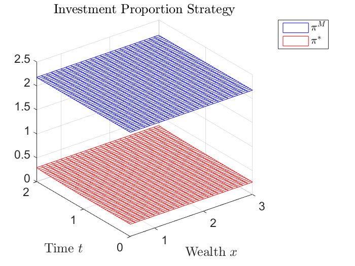
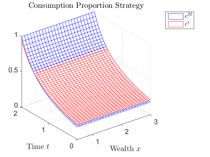
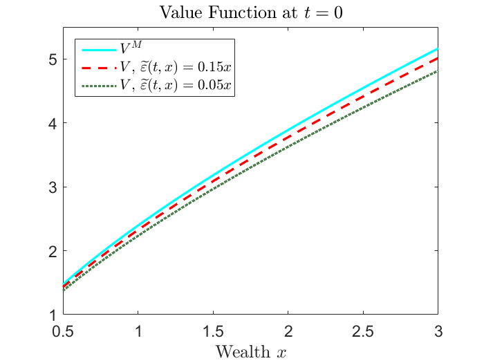
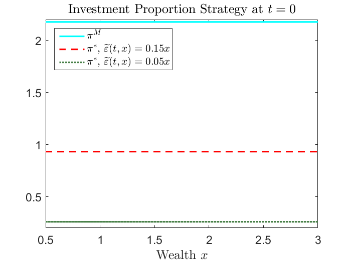
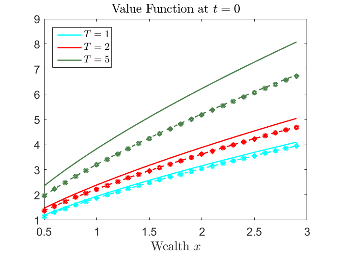
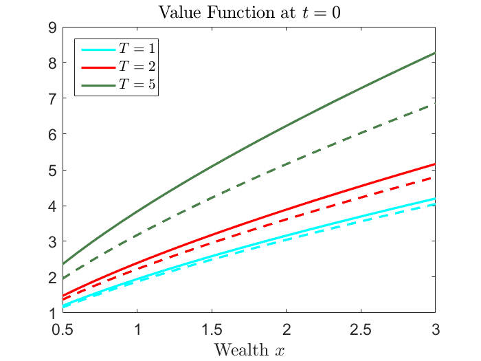
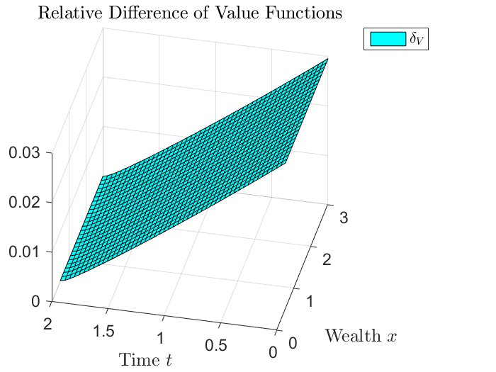
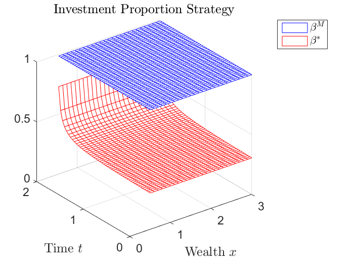
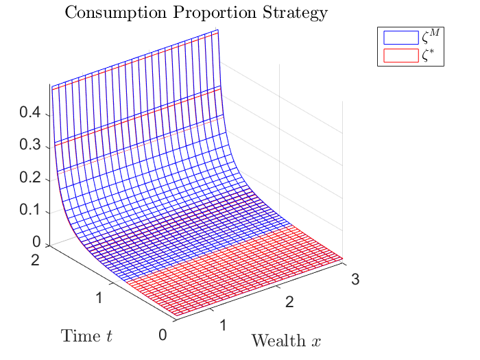
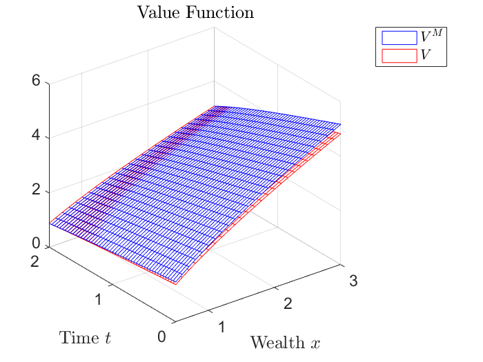
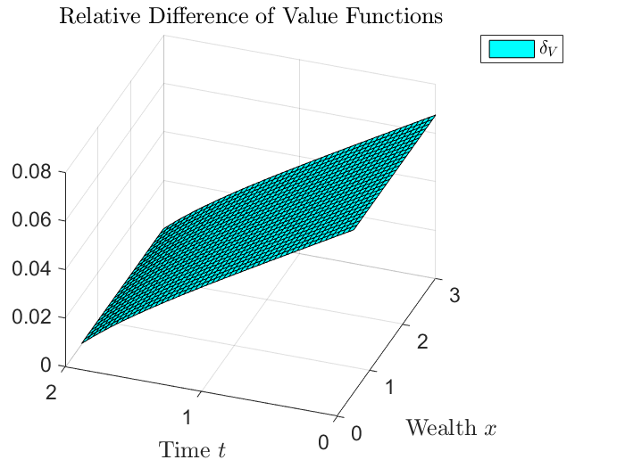
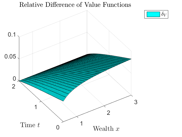
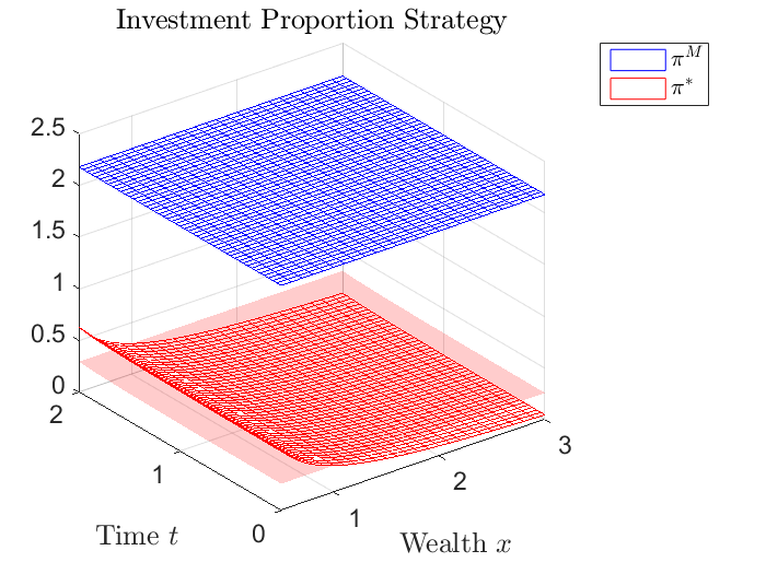
Fig. 1: Effect of the VaR constraint on the value function and optimal portfolio-proportion strategy for the continuous-time problem. The benchmark and bound are given by YtMsuperscriptsubscriptπ‘Œπ‘‘π‘€Y_{t}^{M} and Ξ΅~​(t,x)=0.05​x~πœ€π‘‘π‘₯0.05π‘₯\widetilde{\varepsilon}(t,x)=0.05x, respectively.fig:1

Figure LABEL:fig:1 shows the effect of the VaR constraint on the value function and optimal portfolio-proportion process. The benchmark for the VaR is the conditional expectation of wealth Xt+Ξ”Msuperscriptsubscript𝑋𝑑Δ𝑀X_{t+\Delta}^{M} obtained by an investor following the Merton portfolio-proportion process (Ο€tM,ctM)superscriptsubscriptπœ‹π‘‘π‘€superscriptsubscript𝑐𝑑𝑀(\pi_{t}^{M},c_{t}^{M}) (cf. (LABEL:Merton_strategy)) in [t,t+Ξ”]𝑑𝑑Δ[t,t+\Delta] given the wealth Xt(Ο€,c)superscriptsubscriptπ‘‹π‘‘πœ‹π‘X_{t}^{(\pi,c)} at time t𝑑t, i.e.,

YtM:=𝔼​[Xt+Ξ”M|Xt(Ο€,c)]=Xt(Ο€,c)​exp⁑{(r+Ο€tM​(ΞΌβˆ’r)βˆ’ctM)​Δ}.assignsuperscriptsubscriptπ‘Œπ‘‘π‘€π”Όdelimited-[]conditionalsubscriptsuperscript𝑋𝑀𝑑Δsuperscriptsubscriptπ‘‹π‘‘πœ‹π‘superscriptsubscriptπ‘‹π‘‘πœ‹π‘π‘Ÿsuperscriptsubscriptπœ‹π‘‘π‘€πœ‡π‘Ÿsuperscriptsubscript𝑐𝑑𝑀Δ\displaystyle Y_{t}^{M}:={\mathbb{E}}[X^{M}_{t+\Delta}|X_{t}^{(\pi,c)}]=X_{t}^{(\pi,c)}\exp\left\{\left(r+\pi_{t}^{M}(\mu-r)-c_{t}^{M}\right)\Delta\right\}.

The bound for the VaR is given by Ξ΅~​(t,x)=0.05​x~πœ€π‘‘π‘₯0.05π‘₯\widetilde{\varepsilon}(t,x)=0.05x. This is a bound which is relative to the wealth, i.e., any loss in the interval [t,t+Ξ”]𝑑𝑑Δ[t,t+\Delta] can be hedged with 5% of the portfolio value. By comparison, the risk of the Merton portfolio-proportion process (Ο€tM,ctM)superscriptsubscriptπœ‹π‘‘π‘€superscriptsubscript𝑐𝑑𝑀(\pi_{t}^{M},c_{t}^{M}) which is held constant in [t,t+Ξ”]𝑑𝑑Δ[t,t+\Delta] is Ξ΅~​(t,x)β‰ˆ0.31​x~πœ€π‘‘π‘₯0.31π‘₯\widetilde{\varepsilon}(t,x)\approx 0.31x. A first look at Figure LABEL:fig:1 indicates that the value function and the relative consumption are not remarkably affected by the VaR constraint whereas the proportion of wealth invested in the risky stock is considerably reduced. The top, right-hand panel of Figure LABEL:fig:1 shows the relative difference Ξ΄V​(t,x)subscript𝛿𝑉𝑑π‘₯\delta_{V}(t,x) between the value function of a Merton investor and a VaR-constrained investor defined by

Ξ΄V​(t,x)=VM​(t,x)βˆ’V​(t,x)VM​(t,x).subscript𝛿𝑉𝑑π‘₯superscript𝑉𝑀𝑑π‘₯𝑉𝑑π‘₯superscript𝑉𝑀𝑑π‘₯\displaystyle\delta_{V}(t,x)=\frac{V^{M}(t,x)-V(t,x)}{V^{M}(t,x)}.

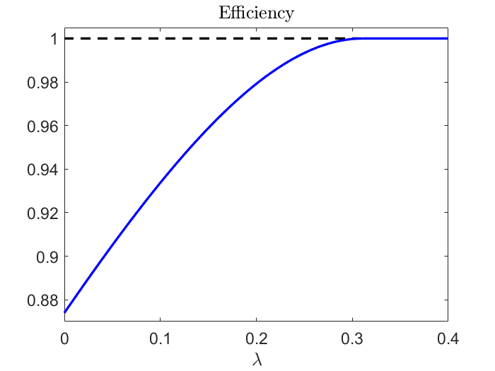
In order to facilitate the comparison of the value functions we express the losses of performance due to the risk constraint in monetary units and introduce the following efficiency measure. The efficiency of an investor A𝐴A relative to an investor B𝐡B is the initial amount of wealth that investor B𝐡B would need to obtain a value function identical to that of investor A𝐴A who started at time t=0𝑑0t=0 with unit wealth. Figure LABEL:fig:eff_con illustrates the efficiency of a VaR-constrained investor relative to a Merton investor in continuous time for different relative bounds of the VaR-constraint. As expected, the efficiency increases when the bound of the risk constraint becomes less restrictive. For the bound Ξ΅~​(t,x)=0.05​x~πœ€π‘‘π‘₯0.05π‘₯\widetilde{\varepsilon}(t,x)=0.05x used in Fig.LABEL:fig:1 the loss of efficiency is about 9.5%. For the most restrictive case, where wealth below the benchmark is not tolerated at all, i.e., the bound is set to Ξ΅~​(t,x)=0~πœ€π‘‘π‘₯0\widetilde{\varepsilon}(t,x)=0, the loss of efficiency is 12.6%.

Refer to caption
Fig. 2: Efficiency of a VaR-constrained investor relative to a Merton investor in continuous time for different relative bounds Ξ΅~​(t,x)=λ​x~πœ€π‘‘π‘₯πœ†π‘₯\widetilde{\varepsilon}(t,x)=\lambda x. The benchmark is given by YtMsubscriptsuperscriptπ‘Œπ‘€π‘‘Y^{M}_{t}.fig:eff_con

Using a relative bound leads to a constant proportion of wealth invested in the risky stock as in the unconstrained case. If we change the relative bound to an absolute one, e.g. Ξ΅~​(t,x)≑0.05~πœ€π‘‘π‘₯0.05\widetilde{\varepsilon}(t,x)\equiv 0.05, the optimal proportion of wealth invested in the risky stock is no longer independent of the wealth level, cf. Figure LABEL:fig:3. This results from the fact that for x<1π‘₯1x<1, the absolute bound is less restrictive and for x>1π‘₯1x>1, it is more restrictive than the relative one. For the optimal relative consumption no remarkable differences between an absolute and a relative bound are observed.
Refer to caption
Refer to caption
Fig. 3: Effect of the VaR constraint on the value function and optimal investment proportion strategy for the continuous-time problem. The benchmark and bound are given by YtMsuperscriptsubscriptπ‘Œπ‘‘π‘€Y_{t}^{M} and Ξ΅~​(t,x)=0.05~πœ€π‘‘π‘₯0.05\widetilde{\varepsilon}(t,x)=0.05, respectively.fig:3
Refer to caption
Refer to caption
Refer to caption
Refer to caption
Fig. 4: Top panels: Effect of different relative bounds (Ξ΅~​(t,x)=0.15​x,0.05​x~πœ€π‘‘π‘₯0.15π‘₯0.05π‘₯\tilde{\varepsilon}(t,x)=0.15x,0.05x) for the VaR constraint on the value function and optimal investment proportion strategy in the continuous-time case. The benchmark and terminal trading time are given by YtMsuperscriptsubscriptπ‘Œπ‘‘π‘€Y_{t}^{M} and T=2𝑇2T=2, respectively.
Bottom panels: Effect of different terminal trading times (T=1,2,5𝑇125T=1,2,5) and different risk constraints (VaR, TCE, EL) on the value function in the continuous-time case. The benchmark is given by YtMsuperscriptsubscriptπ‘Œπ‘‘π‘€Y_{t}^{M}.
Bottom left panel: Value function of the Merton investor (solid line), the VaR-constrained investor (dashed line) and the TCE-constrained investor (asterisk) for Ξ΅~​(t,x)=0.05​x~πœ€π‘‘π‘₯0.05π‘₯\tilde{\varepsilon}(t,x)=0.05x.
Bottom right panel: Value function of the Merton investor (solid line) and the EL-constrained investor (dashed line) for Ξ΅~​(t,x)=0.01​x~πœ€π‘‘π‘₯0.01π‘₯\tilde{\varepsilon}(t,x)=0.01x.fig:4

From the top panels of Figure LABEL:fig:4, we can observe that a more restrictive bound leads to a smaller investment in the risky stock and a smaller value function. Another interesting observation can be made from the bottom panels of Figure LABEL:fig:4. The value function at time t=0𝑑0t=0 is plotted against the wealth level for different terminal trading times T𝑇T. The left panel shows the value function of a Merton investor (solid line), a VaR-constrained investor (dashed line) and a TCE-constrained investor (asterisk). In the right panel, the value function of a Merton investor (solid line) and of a EL-constrained investor (dashed line) is plotted. We observe that the value function is not noticeably affected by the choice of different risk constraints and that there are almost no differences between the VaR constraint and the TCE constraint. This confirms similar results by [7]. Even though a static VaR constraint has been found to induce an increased probability of extreme losses and an increased allocation to risky assets in some states (see [6]), these shortcomings vanish if a VaR constraint is imposed dynamically (cf. [7]).

For longer trading horizons, the effects of a risk constraint on the value function become more noticeable. We obtain comparable results when we change the benchmark to the wealth an investor will obtain at time t+Δ𝑑Δt+\Delta, starting with Xt(Ο€,c)superscriptsubscriptπ‘‹π‘‘πœ‹π‘X_{t}^{(\pi,c)} at time t𝑑t, while only investing in the bond (and not in the stock) and consuming the wealth with the rate ctMsuperscriptsubscript𝑐𝑑𝑀c_{t}^{M} in [t,t+Ξ”]𝑑𝑑Δ[t,t+\Delta], i.e., Yt=Xt(Ο€,c)β‹…e(rβˆ’ctM)​Δ.subscriptπ‘Œπ‘‘β‹…subscriptsuperscriptπ‘‹πœ‹π‘π‘‘superscriptπ‘’π‘Ÿsuperscriptsubscript𝑐𝑑𝑀ΔY_{t}=X^{(\pi,c)}_{t}\cdot e^{(r-c_{t}^{M})\Delta}.

Remark 4.1.

We also performed numerical experiments for the case Ξ³>1𝛾1\gamma>1 instead of Ξ³=0.3𝛾0.3\gamma=0.3 which led to smaller differences between the value function of a Merton investor and a risk-constrained investor. This results from the fact that for a larger γ𝛾\gamma an investor is more risk-averse even without an imposed risk constraint.

4.2 Discrete-time optimization problem

We now consider the discrete-time problem and apply the recursion in Theorem LABEL:DP_Power. The expectation in (LABEL:dp_power) can be written as

𝔼𝔼\displaystyle{\mathbb{E}} [(1+Ξ²Β―β‹…Rtn+1)1βˆ’Ξ³]delimited-[]superscript1⋅¯𝛽subscript𝑅subscript𝑑𝑛11𝛾\displaystyle\left[\left(1+\bar{\beta}\cdot R_{t_{n+1}}\right)^{1-\gamma}\right]
=∫0∞[(1+β¯​(uβˆ’1))1βˆ’Ξ³β‹…12​π​Δ​σ​u​exp⁑{βˆ’(ln⁑uβˆ’(ΞΌβˆ’rβˆ’Οƒ22)​Δ)22​σ2​Δ}]​d​u,absentsuperscriptsubscript0delimited-[]β‹…superscript1¯𝛽𝑒11𝛾12πœ‹Ξ”πœŽπ‘’superscriptπ‘’πœ‡π‘Ÿsuperscript𝜎22Ξ”22superscript𝜎2Ξ”d𝑒\displaystyle=\int_{0}^{\infty}\Big{[}\big{(}1+\bar{\beta}(u-1)\big{)}^{1-\gamma}\cdot\frac{1}{\sqrt{2\pi\Delta}\sigma u}\exp\Big{\{}-\frac{\big{(}\ln u-(\mu-r-\frac{\sigma^{2}}{2})\Delta\big{)}^{2}}{2\sigma^{2}\Delta}\Big{\}}\Big{]}{\text{d}}u,

where we used that Rtn+1=R~tn+1/erβ€‹Ξ”βˆ’1subscript𝑅subscript𝑑𝑛1subscript~𝑅subscript𝑑𝑛1superscriptπ‘’π‘ŸΞ”1R_{t_{n+1}}=\widetilde{R}_{t_{n+1}}/e^{r\Delta}-1 and R~tn+1subscript~𝑅subscript𝑑𝑛1\widetilde{R}_{t_{n+1}} is log-normally distributed. The above integral is evaluated numerically using quadrature rules.
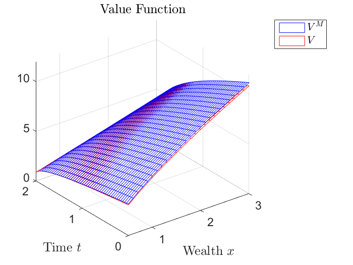
Refer to caption
Refer to caption
Refer to caption
Refer to caption
Fig. 5: Effect of the VaR constraint on the value function and optimal portfolio-proportion strategy in the discrete-time case. The benchmark and bound are given by YtnMsubscriptsuperscriptπ‘Œπ‘€subscript𝑑𝑛Y^{M}_{t_{n}} and Ο΅~​(tn,x)=0.05​x~italic-Ο΅subscript𝑑𝑛π‘₯0.05π‘₯\widetilde{\epsilon}(t_{n},x)=0.05x, respectively. fig:7

Figure LABEL:fig:7 shows the effect of the VaR constraint on the value function and optimal portfolio-proportion strategy. The benchmark for the VaR is the conditional expectation of wealth Xtn+1Msuperscriptsubscript𝑋subscript𝑑𝑛1𝑀X_{t_{n+1}}^{M} obtained by an investor following the (discrete-time) Merton strategy Ο†tnM,Ξ·tnMsuperscriptsubscriptπœ‘subscript𝑑𝑛𝑀superscriptsubscriptπœ‚subscript𝑑𝑛𝑀\varphi_{t_{n}}^{M},\eta_{t_{n}}^{M} given the wealth Xtn(Ο†,Ξ·)superscriptsubscript𝑋subscriptπ‘‘π‘›πœ‘πœ‚X_{t_{n}}^{(\varphi,\eta)} at time tnsubscript𝑑𝑛t_{n}, i.e.,

YtnM=𝔼​[Xtn+1M|Xtn(Ο†,Ξ·)]=er​Δ​(Xtn(Ο†,Ξ·)βˆ’Ξ·tnMβˆ’Ο†tnM)+eμ​Δ​φtnM.subscriptsuperscriptπ‘Œπ‘€subscript𝑑𝑛𝔼delimited-[]conditionalsubscriptsuperscript𝑋𝑀subscript𝑑𝑛1superscriptsubscript𝑋subscriptπ‘‘π‘›πœ‘πœ‚superscriptπ‘’π‘ŸΞ”superscriptsubscript𝑋subscriptπ‘‘π‘›πœ‘πœ‚subscriptsuperscriptπœ‚π‘€subscript𝑑𝑛subscriptsuperscriptπœ‘π‘€subscript𝑑𝑛superscriptπ‘’πœ‡Ξ”subscriptsuperscriptπœ‘π‘€subscript𝑑𝑛\displaystyle Y^{M}_{t_{n}}={\mathbb{E}}[X^{M}_{t_{n+1}}|X_{t_{n}}^{(\varphi,\eta)}]=e^{r\Delta}\left(X_{t_{n}}^{(\varphi,\eta)}-\eta^{M}_{t_{n}}-\varphi^{M}_{t_{n}}\right)+e^{\mu\Delta}\varphi^{M}_{t_{n}}.

The bound for the VaR constraint was given by Ο΅~​(tn,x)=0.05​x~italic-Ο΅subscript𝑑𝑛π‘₯0.05π‘₯\tilde{\epsilon}(t_{n},x)=0.05x. By comparison, the risk of the Merton strategy (Ο†tnM,Ξ·tnM)superscriptsubscriptπœ‘subscript𝑑𝑛𝑀superscriptsubscriptπœ‚subscript𝑑𝑛𝑀(\varphi_{t_{n}}^{M},\eta_{t_{n}}^{M}) is Ο΅~​(t,x)β‰ˆ0.16​x~italic-ϡ𝑑π‘₯0.16π‘₯\widetilde{\epsilon}(t,x)\approx 0.16x. It can be observed that the value function is not remarkably affected by the VaR constraint. Moreover, the effects on the value function are even less notable than in the continuous-time case. This results from the fact that even without an imposed risk constraint short-selling the stock or bond is not allowed, thus the proportion invested in the stock is always in [0,1]01[0,1]. Note that in the above example for the continuous-time problem, the Merton investment proportion is Ο€Mβ‰ˆ2.18superscriptπœ‹π‘€2.18\pi^{M}\approx 2.18, i.e.,it exceeds one. Furthermore, it can be observed from Figure LABEL:fig:7 that the fraction of wealth invested in the risky stock is considerably reduced when the VaR constraint is imposed, whereas the differences in the consumption rate between a VaR-constraint investor and a Merton investor are hard to distinguish visually. If we use an absolute bound Ο΅~​(t,x)≑0.05~italic-ϡ𝑑π‘₯0.05\widetilde{\epsilon}(t,x)\equiv 0.05 for the VaR constraint instead of a relative bound, the optimal investment strategy is no longer a constant proportion of wealth and the results are similar to Figure LABEL:fig:3 for the continuous-time case. Numerical results for varying the terminal trading time or the risk measure are not shown here, but they are comparable to the continuous-time case, cf.Figure LABEL:fig:4.
As in the continuous-time case we now express the losses of performance of a risk-constrained investor relative to the performance of a Merton investor in monetary units using the efficiency measure. The left panel of Figure LABEL:fig:13 illustrates the efficiency of a VaR-constrained investor relative to a Merton investor in discrete time for different relative bounds of the VaR-constraint. As expected and already observed in Fig.LABEL:fig:eff_con, the efficiency increases when the bound of the risk constraint becomes less restrictive. The loss of efficiency is at most 7.2% which is attained for the most restrictive bound, i.e., Ο΅~​(t,x)=0~italic-ϡ𝑑π‘₯0\widetilde{\epsilon}(t,x)=0. For the bound Ο΅~​(t,x)=0.05​x~italic-ϡ𝑑π‘₯0.05π‘₯\widetilde{\epsilon}(t,x)=0.05x used in Fig.LABEL:fig:7 the loss of efficiency is about 4.2%.
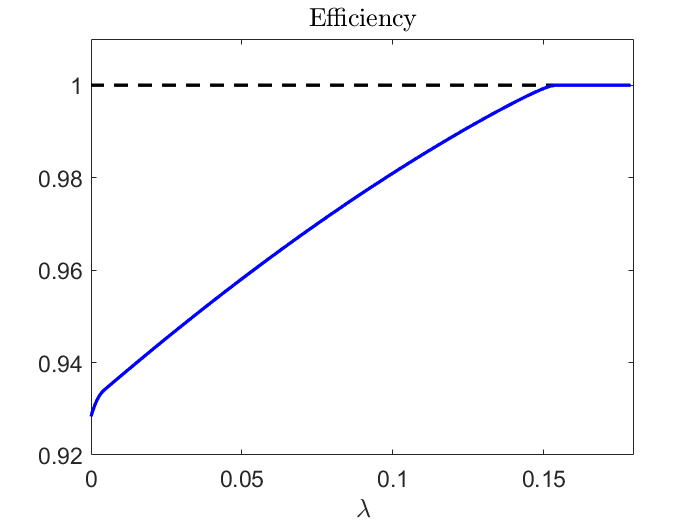
Refer to caption
Refer to caption
Fig. 6: Efficiency for different bounds Ο΅~​(t,x)=λ​x~italic-ϡ𝑑π‘₯πœ†π‘₯\widetilde{\epsilon}(t,x)=\lambda x (left panel) and for different risk measurement horizons ΔΔ\Delta (right panel). The benchmark is given by YtMsubscriptsuperscriptπ‘Œπ‘€π‘‘Y^{M}_{t}.
Left panel: Efficiency of a VaR-constrained investor relative to a Merton investor in discrete time for Ξ³=0.3𝛾0.3\gamma=0.3 and Ξ”=1/24Ξ”124\Delta=1/24.
Right panel: Efficiency of a discrete-time relative to a continuous-time Merton investor and efficiency of a discrete-time relative to a continuous-time VaR-constrained investor for Ξ³=0.9𝛾0.9\gamma=0.9 and Ο΅~​(t,x)=0.05​x~italic-ϡ𝑑π‘₯0.05π‘₯\widetilde{\epsilon}(t,x)=0.05x.fig:13

We finish this section with a numerical comparison of the continuous-time and discrete-time case. The availability of solutions to the risk-constrained portfolio problem both for discrete and continuous time allows us to quantify the losses of portfolio performance resulting from time discretization, i.e.,from the restriction to finite trading frequencies. First observe that the loss of efficiency resulting from imposing a risk-constraint is higher in continuous time than in discrete time, cf. Figure LABEL:fig:eff_con and left panel of Figure LABEL:fig:13. This arises from the fact that short-selling is allowed in continuous time leading to Ο€Mβ‰ˆ2.18>1superscriptπœ‹π‘€2.181\pi^{M}\approx 2.18>1 whereas it is not allowed in discrete time leading to Ξ²M=1superscript𝛽𝑀1\beta^{M}=1. For a fair comparison we do not allow for short-selling in both cases. Since the parameters of the financial market shall remain the same, we change the investors' preferences represented by the utility functions by setting Ξ³=0.9𝛾0.9\gamma=0.9. This leads to Ο€M,Ξ²M∈[0,1]superscriptπœ‹π‘€superscript𝛽𝑀01\pi^{M},\,\beta^{M}\in[0,1], i.e., there is no short-selling in both cases. Furthermore, the expected utility from consumption in the time interval [tn,tn+1)subscript𝑑𝑛subscript𝑑𝑛1[t_{n},t_{n+1}), n=0,…,Nβˆ’1𝑛0…𝑁1n=0,\ldots,N-1, is given by 𝔼​[∫tntn+1U1​(Cs)​d​s]𝔼delimited-[]superscriptsubscriptsubscript𝑑𝑛subscript𝑑𝑛1subscriptπ‘ˆ1subscript𝐢𝑠d𝑠{\mathbb{E}}[\int_{t_{n}}^{t_{n+1}}U_{1}(C_{s}){\text{d}}s] in the continuous-time case. However, in the discrete-time case we have 𝔼​[U1​(Ξ·tn)]𝔼delimited-[]subscriptπ‘ˆ1subscriptπœ‚subscript𝑑𝑛{\mathbb{E}}[U_{1}(\eta_{t_{n}})], which approximately corresponds to 𝔼​[U1​(∫tntn+1Cs​d​s)]𝔼delimited-[]subscriptπ‘ˆ1superscriptsubscriptsubscript𝑑𝑛subscript𝑑𝑛1subscript𝐢𝑠d𝑠{\mathbb{E}}[U_{1}(\int_{t_{n}}^{t_{n+1}}C_{s}{\text{d}}s)]. The related maximization problem

o​p​2​𝔼t0,x0​[U1​(∫0TCt​d​t)+U2​(XTu)]π‘œπ‘2subscript𝔼subscript𝑑0subscriptπ‘₯0delimited-[]subscriptπ‘ˆ1superscriptsubscript0𝑇subscript𝐢𝑑d𝑑subscriptπ‘ˆ2subscriptsuperscript𝑋𝑒𝑇\displaystyle{op2}\mathbb{E}_{t_{0},x_{0}}\Big{[}U_{1}\Big{(}\int_{0}^{T}C_{t}{\text{d}}\,t\Big{)}+U_{2}(X^{u}_{T})\Big{]}

is not only different from the economic interpretation, but also from the mathematical point of view, cf. Grandits et al. [11]. Since we want to quantify the losses of portfolio performance resulting solely from restricting to finite trading frequencies, we set U1​(x)≑0subscriptπ‘ˆ1π‘₯0U_{1}(x)\equiv 0. Again, we use the efficiency to compare the portfolio performance of a discrete-time investor relative to a continuous-time investor with and without imposing a risk constraint. For this experiment, we compute the VaR risk measure for the continuous-time investor under the assumption that the number of shares remains constant between t𝑑t and t+Δ𝑑Δt+\Delta. In Rogers [22] the continuous-time investment problem is compared to the discrete-time investment problem when no risk constraint is imposed. The author shows that there is only a small difference between the continuous and discrete problem when the additional restriction that the continuous-time investor is not allowed to sell short the stock or the bond is imposed. BΓ€uerle et al. [4] show that this remains true for models where the drift is modeled by a random variable that is not directly observable and has to be estimated from observed stock prices. However, the authors found that when the short-selling restriction for the continuous-time investor is omitted, the discrete-time investor will generally not do as well as the continuous-time investor and a discretization gap remains. The right panel of Figure LABEL:fig:13 shows the efficiency of a discrete-time relative to a continuous-time Merton investor (cyan) and the efficiency of a discrete-time relative to a continuous-time VaR-constrained investor (red). We observe that the values of the efficiency are very close to unity; even for a quite large ΔΔ\Delta in the range of 2.52.52.5 years, the loss of efficiency is at most 0.35%percent0.350.35\% in both cases. This is in line with the results by Rogers [22] for the Merton investor. In addition to the results in [22] our numerical results for the risk-constrained case indicate that the losses due to time discretization are of comparable (small) magnitude.

References

  • [1] Akume, D. (2007): Risk-Constrained Dynamic Portfolio Management. Ph.D. thesis, University of Yaounde I.
  • [2] Akume, D.; Luderer, B. and Wunderlich, R. (2010): Dynamic shortfall constraints for optimal portfolios. Surveys in Mathematics and its Applications, 5, 135-149.
  • [3] Artzner, P.; Delbaen, F.; Eber, J. and Heath, D. (1999): Coherent Measures of Risk. Mathematical Finance, 9 (3), 203-228.
  • [4] BΓ€uerle, N.; Urban, S. and Veraart, L. A. M. (2012): The relaxed investor with partial information. SIAM Journal on Financial Mathematics, 3 (1), 304-327.
  • [5] BΓ€uerle, N.; Rieder, U. (2011): Markov Decision Processes with Applications to Finance. Springer, Berlin.
  • [6] Basak, S.; Shapiro, A. (2001): Value-at-risk-based risk management: optimal policies and asset prices, Rev. Financial Studies 14, 371–405.
  • [7] Cuoco, D.; He, H. and Issaenko, S. (2008): Optimal Dynamic Trading Strategies with Risk Limits. Operations Research, 56 (2), 358-368.
  • [8] Duffy, D. (2006): Finite Difference Methods in Financial Engineering: A Partial Differential Equation Approach. Wiley, Chichester.
  • [9] Fleming, W. H. and Soner, H. M. (2006): Controlled Markov Processes and Viscosity Solutions, 2nd edn, Springer, New York.
  • [10] Gabih, A.; Sass, J. and Wunderlich, R. (2009): Utility maximization under bounded expected loss. Stochastic Models, 25, 375-409.
  • [11] Grandits P., Hubalek F., Schachermayer W. and Ε½igo, M. (2007): Optimal expected exponential utility of dividend payments in a Brownian risk model. Scandinavian Actuarial Journal, 2, 73-107.
  • [12] Hinderer, K. (1970): Foundations of non-stationary dynamic programming with discrete time parameter. Springer, Berlin.
  • [13] Jichun L.; Yi-Tung, C. (2008): Computational Partial Differential Equations Using MATLAB. CRC Press, Boca Raton.
  • [14] Jorion, P. (2001): Value at Risk. McGraw-Hill, New York.
  • [15] Korn, R. (1997): Optimal Portfolios. World Scientific, Singapore.
  • [16] Leippold, M., Trojani, F., Vanini, P. (2006): Equilibrium impact of value-at-risk regulation. Journal of Economic Dynamics and Control 30(8), 1277-1313.
  • [17] Moreno-Bromberg, S., Pirvu, T. A., RΓ©veillac, A. (2013): CRRA utility maximization under dynamic risk constraints. Communications on Stochastic Analysis 7 (2), 203-225.
  • [18] Nocedal J.; Wright, S. J. (2006): Numerical Optimization. 2nd edn, Springer, New York.
  • [19] Pham, H. (2009): Continuous-time Stochastic Control and Optimization with Financial Applications. Springer, Berlin.
  • [20] Pirvu, T. A. (2007): Portfolio optimization under the Value-at-Risk constraint. Quantitative Finance, 7, 125-136.
  • [21] PutschΓΆgl, W. and Sass, J. (2008): Optimal consumption and investment under partial information. Decisions in Economics and Finance 31, 131–170.
  • [22] Rogers, L. C. G. (2001): The relaxed investor and parameter uncertainty. Finance and Stochastics, 5, 131-154.
  • [23] Shardin, A. A.; Wunderlich, R. (2017): Partially Observable Stochastic Optimal Control Problems for an Energy Storage. Stochastics, 89 (1), 280-310.
  • [24] Yiu, K. F. C. (2004): Optimal portfolios under a value-at-risk constraint. Journal of Economic Dynamics and Control, 28 (7), 1317-1334.

Appendix A Proof of Lemma LABEL:lem:risk_measures

appA Under the assumption that the portfolio-proportion strategy (𝝅,c)𝝅𝑐(\boldsymbol{\pi},c) is kept constant and equal to (𝝅¯,cΒ―)¯𝝅¯𝑐(\bar{\boldsymbol{\pi}},\bar{c}) between time t𝑑t and t+Δ𝑑Δt+\Delta the wealth at time t+Δ𝑑Δt+\Delta is given by

Xt+Ξ”=exp{\displaystyle X_{t+\Delta}=\exp\Big{\{} ln⁑(Xt)+(𝝅¯′​(πβˆ’πŸβ€‹r)+rβˆ’cΒ―βˆ’βˆ₯π…Β―β€²β€‹πˆβˆ₯22)​Δsubscript𝑋𝑑superscript¯𝝅′𝝁1π‘Ÿπ‘ŸΒ―π‘superscriptdelimited-βˆ₯βˆ₯superscriptΒ―π…β€²πˆ22Ξ”\displaystyle\ln\big{(}X_{t}\big{)}+\Big{(}\bar{\boldsymbol{\pi}}^{\prime}(\boldsymbol{\mu}-{\mathbf{1}}r)+r-\bar{c}-\frac{\lVert\bar{\boldsymbol{\pi}}^{\prime}\boldsymbol{\sigma}\rVert^{2}}{2}\Big{)}\Delta
+π…Β―β€²πˆ(𝑾t+Ξ”βˆ’π‘Ύt)}.\displaystyle+\bar{\boldsymbol{\pi}}^{\prime}\boldsymbol{\sigma}(\boldsymbol{W}_{t+\Delta}-\boldsymbol{W}_{t})\Big{\}}.

From the equation above we obtain that Xt+Ξ”subscript𝑋𝑑ΔX_{t+\Delta} is - conditionally on β„±tsubscriptℱ𝑑{\cal F}_{t} - distributed as eZsuperscript𝑒𝑍e^{Z}, where Z𝑍Z is normally distributed with mean mπ‘šm and variance s2superscript𝑠2s^{2}. Here,

m:=ln⁑(Xt)+(𝝅¯′​(πβˆ’πŸβ€‹r)+rβˆ’cΒ―βˆ’12​βˆ₯π…Β―β€²β€‹πˆβˆ₯2)​Δands2:=βˆ₯π…Β―β€²β€‹πˆβˆ₯2​Δ.formulae-sequenceassignπ‘šsubscript𝑋𝑑superscript¯𝝅′𝝁1π‘Ÿπ‘ŸΒ―π‘12superscriptdelimited-βˆ₯βˆ₯superscriptΒ―π…β€²πˆ2Ξ”andassignsuperscript𝑠2superscriptdelimited-βˆ₯βˆ₯superscriptΒ―π…β€²πˆ2Ξ”\displaystyle m:=\ln\left(X_{t}\right)+\Big{(}\bar{\boldsymbol{\pi}}^{\prime}(\boldsymbol{\mu}-{\mathbf{1}}r)+r-\bar{c}-\frac{1}{2}\lVert\bar{\boldsymbol{\pi}}^{\prime}\boldsymbol{\sigma}\rVert^{2}\Big{)}\Delta\quad\text{and}\quad s^{2}:=\lVert\bar{\boldsymbol{\pi}}^{\prime}\boldsymbol{\sigma}\rVert^{2}\Delta.

Recall, the Expected Loss at time t𝑑t is defined by

ELt​(Lt):=𝔼​[(Ytβˆ’Xt+Ξ”)+|β„±t]=𝔼​[(Ytβˆ’eZ)+|β„±t].assignsubscriptEL𝑑subscript𝐿𝑑𝔼delimited-[]conditionalsuperscriptsubscriptπ‘Œπ‘‘subscript𝑋𝑑Δsubscriptℱ𝑑𝔼delimited-[]conditionalsuperscriptsubscriptπ‘Œπ‘‘superscript𝑒𝑍subscriptℱ𝑑\displaystyle\text{EL}_{t}\left(L_{t}\right):={\mathbb{E}}\Big{[}\left(Y_{t}-X_{t+\Delta}\right)^{+}\Big{|}\,\,{\cal F}_{t}\Big{]}={\mathbb{E}}\Big{[}\left(Y_{t}-e^{Z}\right)^{+}\Big{|}\,\,{\cal F}_{t}\Big{]}.

This expectation can be calculated as follows. Let

fZ​(z)=12​π​s​exp⁑(βˆ’(zβˆ’m)22​s2)subscript𝑓𝑍𝑧12πœ‹π‘ superscriptπ‘§π‘š22superscript𝑠2\displaystyle f_{Z}(z)=\frac{1}{\sqrt{2\pi}s}\exp{\Big{(}-\frac{(z-m)^{2}}{2s^{2}}\Big{)}}

denote the probability density function of Z𝑍Z then

ELt​(Lt)subscriptEL𝑑subscript𝐿𝑑\displaystyle\text{EL}_{t}\left(L_{t}\right) =βˆ«βˆ’βˆžβˆž(Ytβˆ’ez)+​fZ​(z)​d​z=βˆ«βˆ’βˆžln⁑(Yt)(Ytβˆ’ez)​fZ​(z)​d​z=Yt​I1+I2,absentsuperscriptsubscriptsuperscriptsubscriptπ‘Œπ‘‘superscript𝑒𝑧subscript𝑓𝑍𝑧d𝑧superscriptsubscriptsubscriptπ‘Œπ‘‘subscriptπ‘Œπ‘‘superscript𝑒𝑧subscript𝑓𝑍𝑧d𝑧subscriptπ‘Œπ‘‘subscript𝐼1subscript𝐼2\displaystyle=\int\nolimits_{-\infty}^{\infty}{\left(Y_{t}-e^{z}\right)^{+}f_{Z}(z){\text{d}}z}=\int\nolimits_{-\infty}^{\ln(Y_{t})}{\left(Y_{t}-e^{z}\right)f_{Z}(z){\text{d}}z}=Y_{t}I_{1}+I_{2},

where I1:=βˆ«βˆ’βˆžln⁑(Yt)fZ​(z)​d​z​ and ​I2:=βˆ’βˆ«βˆ’βˆžln⁑(Yt)ez​fZ​(z)​d​z.assignsubscript𝐼1superscriptsubscriptsubscriptπ‘Œπ‘‘subscript𝑓𝑍𝑧d𝑧 andΒ subscript𝐼2assignsuperscriptsubscriptsubscriptπ‘Œπ‘‘superscript𝑒𝑧subscript𝑓𝑍𝑧d𝑧I_{1}:=\int_{-\infty}^{\ln(Y_{t})}f_{Z}(z){\text{d}}z\text{ and }I_{2}:=-\int_{-\infty}^{\ln(Y_{t})}e^{z}f_{Z}(z){\text{d}}z.
For the integral I1subscript𝐼1I_{1} an appropriate change of variables yields

I1=βˆ«βˆ’βˆžd112​π​eβˆ’y22​d​y=Φ​(d1),subscript𝐼1superscriptsubscriptsubscript𝑑112πœ‹superscript𝑒superscript𝑦22d𝑦Φsubscript𝑑1\displaystyle I_{1}=\int\nolimits_{-\infty}^{d_{1}}{\frac{1}{\sqrt{2\pi}}e^{-\frac{y^{2}}{2}}{\text{d}}y}=\Phi(d_{1}),

where

d1::subscript𝑑1absent\displaystyle d_{1}: =ln⁑(Yt)βˆ’ms=1βˆ₯π…Β―β€²β€‹πˆβˆ₯​Δ​[ln⁑(YtXt)βˆ’(𝝅¯′​(πβˆ’πŸβ€‹r)+rβˆ’cΒ―βˆ’βˆ₯π…Β―β€²β€‹πˆβˆ₯22)​Δ]absentsubscriptπ‘Œπ‘‘π‘šπ‘ 1delimited-βˆ₯βˆ₯superscriptΒ―π…β€²πˆΞ”delimited-[]subscriptπ‘Œπ‘‘subscript𝑋𝑑superscript¯𝝅′𝝁1π‘Ÿπ‘ŸΒ―π‘superscriptdelimited-βˆ₯βˆ₯superscriptΒ―π…β€²πˆ22Ξ”\displaystyle=\frac{\ln(Y_{t})-m}{s}=\frac{1}{\lVert\bar{\boldsymbol{\pi}}^{\prime}\boldsymbol{\sigma}\rVert\sqrt{\Delta}}\Big{[}\ln\Big{(}\frac{Y_{t}}{X_{t}}\Big{)}-\big{(}\bar{\boldsymbol{\pi}}^{\prime}(\boldsymbol{\mu}-{\mathbf{1}}r)+r-\bar{c}-\frac{\lVert\bar{\boldsymbol{\pi}}^{\prime}\boldsymbol{\sigma}\rVert^{2}}{2}\big{)}\Delta\Big{]}

and Φ​(β‹…)Ξ¦β‹…\Phi(\cdot) denotes the cumulative distribution function of the standard normal distribution. The integral I2subscript𝐼2I_{2} can be written as

I2subscript𝐼2\displaystyle I_{2} =βˆ’βˆ«βˆ’βˆžln⁑(Yt)12​π​s​exp⁑(zβˆ’z2βˆ’2​z​m+m22​s2)​d​zabsentsuperscriptsubscriptsubscriptπ‘Œπ‘‘12πœ‹π‘ π‘§superscript𝑧22π‘§π‘šsuperscriptπ‘š22superscript𝑠2d𝑧\displaystyle=-\int\nolimits_{-\infty}^{\ln(Y_{t})}{\frac{1}{\sqrt{2\pi}s}\exp{\Big{(}z-\frac{z^{2}-2zm+m^{2}}{2s^{2}}\Big{)}}{\text{d}}z}
=βˆ’es22+mβ€‹βˆ«βˆ’βˆžln⁑(Yt)12​π​s​exp⁑(βˆ’(zβˆ’(m+s2))22​s2)​d​z.absentsuperscript𝑒superscript𝑠22π‘šsuperscriptsubscriptsubscriptπ‘Œπ‘‘12πœ‹π‘ superscriptπ‘§π‘šsuperscript𝑠222superscript𝑠2d𝑧\displaystyle=-e^{\frac{s^{2}}{2}+m}\int\nolimits_{-\infty}^{\ln(Y_{t})}{\frac{1}{\sqrt{2\pi}s}\exp{\Big{(}-\frac{\left(z-(m+s^{2})\right)^{2}}{2s^{2}}\Big{)}}{\text{d}}z}.

Using the change of variables technique yields

I2subscript𝐼2\displaystyle I_{2} =βˆ’es22+mβ€‹βˆ«βˆ’βˆžd212​π​eβˆ’y22​d​y=βˆ’es22+m​Φ​(d2),absentsuperscript𝑒superscript𝑠22π‘šsuperscriptsubscriptsubscript𝑑212πœ‹superscript𝑒superscript𝑦22d𝑦superscript𝑒superscript𝑠22π‘šΞ¦subscript𝑑2\displaystyle=-e^{\frac{s^{2}}{2}+m}\int\nolimits_{-\infty}^{d_{2}}{\frac{1}{\sqrt{2\pi}}e^{-\frac{y^{2}}{2}}{\text{d}}y}=-e^{\frac{s^{2}}{2}+m}\Phi(d_{2}),

where

d2::subscript𝑑2absent\displaystyle d_{2}: =ln⁑(Yt)βˆ’(m+s2)sabsentsubscriptπ‘Œπ‘‘π‘šsuperscript𝑠2𝑠\displaystyle=\frac{\ln(Y_{t})-(m+s^{2})}{s}
=1βˆ₯π…Β―β€²β€‹πˆβˆ₯​Δ​[ln⁑(f~​(t,Xt)Xt)βˆ’(𝝅¯′​(πβˆ’πŸβ€‹r)+rβˆ’cΒ―+12​βˆ₯π…Β―β€²β€‹πˆβˆ₯2)​Δ].absent1delimited-βˆ₯βˆ₯superscriptΒ―π…β€²πˆΞ”delimited-[]~𝑓𝑑subscript𝑋𝑑subscript𝑋𝑑superscript¯𝝅′𝝁1π‘Ÿπ‘ŸΒ―π‘12superscriptdelimited-βˆ₯βˆ₯superscriptΒ―π…β€²πˆ2Ξ”\displaystyle=\frac{1}{\lVert\bar{\boldsymbol{\pi}}^{\prime}\boldsymbol{\sigma}\rVert\sqrt{\Delta}}\bigg{[}\ln\Big{(}\frac{\widetilde{f}(t,X_{t})}{X_{t}}\Big{)}-\Big{(}\bar{\boldsymbol{\pi}}^{\prime}(\boldsymbol{\mu}-{\mathbf{1}}r)+r-\bar{c}+\frac{1}{2}\lVert\bar{\boldsymbol{\pi}}^{\prime}\boldsymbol{\sigma}\rVert^{2}\Big{)}\Delta\bigg{]}.

Note, exp⁑{s2/2+m}=Xt​exp⁑((𝝅¯′​(πβˆ’πŸβ€‹r)+rβˆ’cΒ―)​Δ)superscript𝑠22π‘šsubscript𝑋𝑑superscript¯𝝅′𝝁1π‘Ÿπ‘ŸΒ―π‘Ξ”\exp\{s^{2}/2+m\}=X_{t}\exp{\left(\left(\bar{\boldsymbol{\pi}}^{\prime}(\boldsymbol{\mu}-{\mathbf{1}}r)+r-\bar{c}\right)\Delta\right)}. Finally we obtain

ELt​(Lt)=Yt​I1+I2=f~​(t,Xt)​Φ​(d1)βˆ’Xt​exp⁑((𝝅¯′​(πβˆ’πŸβ€‹r)+rβˆ’cΒ―)​Δ)​Φ​(d2).subscriptEL𝑑subscript𝐿𝑑subscriptπ‘Œπ‘‘subscript𝐼1subscript𝐼2~𝑓𝑑subscript𝑋𝑑Φsubscript𝑑1subscript𝑋𝑑superscript¯𝝅′𝝁1π‘Ÿπ‘ŸΒ―π‘Ξ”Ξ¦subscript𝑑2\displaystyle\text{EL}_{t}\left(L_{t}\right)=Y_{t}I_{1}+I_{2}=\widetilde{f}(t,X_{t})\Phi(d_{1})-X_{t}\exp{\left(\left(\bar{\boldsymbol{\pi}}^{\prime}(\boldsymbol{\mu}-{\mathbf{1}}r)+r-\bar{c}\right)\Delta\right)}\Phi(d_{2}).

Appendix B Proof of Lemma LABEL:lem:risk_measures_discrete

appB Given an investment-consumption strategy (Ο†,Ξ·)πœ‘πœ‚(\varphi,\eta) the wealth process X𝑋X evolves as follows

Xtn+1subscript𝑋subscript𝑑𝑛1\displaystyle X_{t_{n+1}} =er​Δ​(Xtnβˆ’Ξ·tnβˆ’Ο†tn)+Ο†tnβ‹…exp⁑{(ΞΌβˆ’Οƒ22)​Δ+σ​(Wtn+1βˆ’Wtn)}.absentsuperscriptπ‘’π‘ŸΞ”subscript𝑋subscript𝑑𝑛subscriptπœ‚subscript𝑑𝑛subscriptπœ‘subscript𝑑𝑛⋅subscriptπœ‘subscriptπ‘‘π‘›πœ‡superscript𝜎22Ξ”πœŽsubscriptπ‘Šsubscript𝑑𝑛1subscriptπ‘Šsubscript𝑑𝑛\displaystyle=e^{r\Delta}(X_{t_{n}}-\eta_{t_{n}}-\varphi_{t_{n}})+\varphi_{t_{n}}\cdot\exp\big{\{}\big{(}\mu-\frac{\sigma^{2}}{2}\big{)}\Delta+\sigma\big{(}W_{t_{n+1}}-W_{t_{n}}\big{)}\big{\}}.

Note that given a probability level α∈(0,1)𝛼01\alpha\in(0,1) the Value at Risk at time tnsubscript𝑑𝑛t_{n} is defined by VaRtnα​(Ltn):=inf{lβˆˆβ„|P​(Ltnβ‰₯l|𝒒tn)≀α}.assignsuperscriptsubscriptVaRsubscript𝑑𝑛𝛼subscript𝐿subscript𝑑𝑛infimumconditional-set𝑙ℝ𝑃subscript𝐿subscript𝑑𝑛conditional𝑙subscript𝒒subscript𝑑𝑛𝛼\text{VaR}_{t_{n}}^{\alpha}(L_{t_{n}}):=\inf\left\{l\in{\mathbb{R}}\,|\,{P}(L_{t_{n}}\geq l|{\cal G}_{t_{n}})\leq\alpha\right\}. We have

Ltn=Ytnβˆ’Xtn+1subscript𝐿subscript𝑑𝑛subscriptπ‘Œsubscript𝑑𝑛subscript𝑋subscript𝑑𝑛1\displaystyle L_{t_{n}}=Y_{t_{n}}-X_{t_{n+1}} =f~​(tn,Xtn)βˆ’er​Δ​(Xtnβˆ’Ξ·tnβˆ’Ο†tn)absent~𝑓subscript𝑑𝑛subscript𝑋subscript𝑑𝑛superscriptπ‘’π‘ŸΞ”subscript𝑋subscript𝑑𝑛subscriptπœ‚subscript𝑑𝑛subscriptπœ‘subscript𝑑𝑛\displaystyle=\widetilde{f}(t_{n},X_{t_{n}})-e^{r\Delta}(X_{t_{n}}-\eta_{t_{n}}-\varphi_{t_{n}})
βˆ’Ο†tnβ‹…exp⁑{(ΞΌβˆ’Οƒ22)​Δ+σ​(Wtn+1βˆ’Wtn)}β‹…subscriptπœ‘subscriptπ‘‘π‘›πœ‡superscript𝜎22Ξ”πœŽsubscriptπ‘Šsubscript𝑑𝑛1subscriptπ‘Šsubscript𝑑𝑛\displaystyle-\varphi_{t_{n}}\cdot\exp\Big{\{}\Big{(}\mu-\frac{\sigma^{2}}{2}\Big{)}\Delta+\sigma\left(W_{t_{n+1}}-W_{t_{n}}\right)\Big{\}}

and

P​(Ltnβ‰₯l|𝒒tn)𝑃subscript𝐿subscript𝑑𝑛conditional𝑙subscript𝒒subscript𝑑𝑛\displaystyle{P}\left(L_{t_{n}}\geq l|{\cal G}_{t_{n}}\right) =P(exp{(ΞΌβˆ’Οƒ22)Ξ”+Οƒ(Wtn+1βˆ’Wtn)}\displaystyle={P}\Big{(}\exp\Big{\{}\Big{(}\mu-\frac{\sigma^{2}}{2}\Big{)}\Delta+\sigma\left(W_{t_{n+1}}-W_{t_{n}}\right)\Big{\}}
≀f~​(tn,Xtn)βˆ’er​Δ​(Xtnβˆ’Ξ·tnβˆ’Ο†tn)βˆ’lΟ†tn|𝒒tn)\displaystyle\qquad\leq\frac{\widetilde{f}(t_{n},X_{t_{n}})-e^{r\Delta}(X_{t_{n}}-\eta_{t_{n}}-\varphi_{t_{n}})-l}{\varphi_{t_{n}}}\Big{|}{\cal G}_{t_{n}}\Big{)}
=P​(Ξ”βˆ’12​(Wtn+1βˆ’Wtn)≀z|𝒒tn)=Φ​(z),absent𝑃superscriptΞ”12subscriptπ‘Šsubscript𝑑𝑛1subscriptπ‘Šsubscript𝑑𝑛conditional𝑧subscript𝒒subscript𝑑𝑛Φ𝑧\displaystyle={P}\big{(}\Delta^{-\frac{1}{2}}\big{(}W_{t_{n+1}}-W_{t_{n}}\big{)}\leq z\big{|}{\cal G}_{t_{n}}\big{)}=\Phi(z),

where

z=1σ​Δ​(ln⁑{f~​(tn,Xtn)βˆ’er​Δ​(Xtnβˆ’Ξ·tnβˆ’Ο†tn)βˆ’lΟ†tn}βˆ’(ΞΌβˆ’Οƒ22)​Δ).𝑧1πœŽΞ”~𝑓subscript𝑑𝑛subscript𝑋subscript𝑑𝑛superscriptπ‘’π‘ŸΞ”subscript𝑋subscript𝑑𝑛subscriptπœ‚subscript𝑑𝑛subscriptπœ‘subscript𝑑𝑛𝑙subscriptπœ‘subscriptπ‘‘π‘›πœ‡superscript𝜎22Ξ”\displaystyle z=\frac{1}{\sigma\sqrt{\Delta}}\Big{(}\ln\Big{\{}\frac{\widetilde{f}(t_{n},X_{t_{n}})-e^{r\Delta}(X_{t_{n}}-\eta_{t_{n}}-\varphi_{t_{n}})-l}{\varphi_{t_{n}}}\Big{\}}-\big{(}\mu-\frac{\sigma^{2}}{2}\big{)}\Delta\Big{)}.

We have used that the random variable Ξ”βˆ’12​(Wtn+1βˆ’Wtn)superscriptΞ”12subscriptπ‘Šsubscript𝑑𝑛1subscriptπ‘Šsubscript𝑑𝑛\Delta^{-\frac{1}{2}}(W_{t_{n+1}}-W_{t_{n}}) is standard normally distributed and independent of 𝒒tnsubscript𝒒subscript𝑑𝑛{\cal G}_{t_{n}}. Thus, P​(Ltnβ‰₯l|𝒒tn)=Φ​(z)≀α𝑃subscript𝐿subscript𝑑𝑛conditional𝑙subscript𝒒subscript𝑑𝑛Φ𝑧𝛼{P}\left(L_{t_{n}}\geq l|{\cal G}_{t_{n}}\right)=\Phi(z)\leq\alpha is satisfied for zβ‰€Ξ¦βˆ’1​(Ξ±)𝑧superscriptΞ¦1𝛼z\leq\Phi^{-1}(\alpha) yielding

lβ‰₯f~​(tn,Xtn)βˆ’er​Δ​(Xtnβˆ’Ξ·tnβˆ’Ο†tn)βˆ’exp⁑{Ξ¦βˆ’1​(Ξ±)​σ​Δ+(ΞΌβˆ’Οƒ22)​Δ}​φtn.𝑙~𝑓subscript𝑑𝑛subscript𝑋subscript𝑑𝑛superscriptπ‘’π‘ŸΞ”subscript𝑋subscript𝑑𝑛subscriptπœ‚subscript𝑑𝑛subscriptπœ‘subscript𝑑𝑛superscriptΞ¦1π›ΌπœŽΞ”πœ‡superscript𝜎22Ξ”subscriptπœ‘subscript𝑑𝑛\displaystyle l\geq\widetilde{f}(t_{n},X_{t_{n}})-e^{r\Delta}(X_{t_{n}}-\eta_{t_{n}}-\varphi_{t_{n}})-\exp\big{\{}\Phi^{-1}(\alpha)\sigma\sqrt{\Delta}+\big{(}\mu-\frac{\sigma^{2}}{2}\big{)}\Delta\big{\}}\varphi_{t_{n}}.

Since the Dynamic Value at Risk is the smallest l𝑙l satisfying the above inequality we obtain VaRtnα​(Ltn)=ψ~​(tn,Xtn,Ο†tn,Ξ·tn)subscriptsuperscriptVaR𝛼subscript𝑑𝑛subscript𝐿subscript𝑑𝑛~πœ“subscript𝑑𝑛subscript𝑋subscript𝑑𝑛subscriptπœ‘subscript𝑑𝑛subscriptπœ‚subscript𝑑𝑛\text{VaR}^{\alpha}_{t_{n}}(L_{t_{n}})=\widetilde{\psi}(t_{n},X_{t_{n}},\varphi_{t_{n}},\eta_{t_{n}}), where

ψ~​(t,x,φ¯,Ξ·Β―)=~πœ“π‘‘π‘₯Β―πœ‘Β―πœ‚absent\displaystyle\widetilde{\psi}(t,x,\bar{\varphi},\bar{\eta})= f~​(t,x)βˆ’er​Δ​(xβˆ’Ξ·Β―βˆ’Ο†Β―)βˆ’exp⁑{Ξ¦βˆ’1​(Ξ±)​σ​Δ+(ΞΌβˆ’Οƒ22)​Δ}​φ¯.~𝑓𝑑π‘₯superscriptπ‘’π‘ŸΞ”π‘₯Β―πœ‚Β―πœ‘superscriptΞ¦1π›ΌπœŽΞ”πœ‡superscript𝜎22Ξ”Β―πœ‘\displaystyle\widetilde{f}(t,x)-e^{r\Delta}(x-\bar{\eta}-\bar{\varphi})-\exp\Big{\{}\Phi^{-1}(\alpha)\sigma\sqrt{\Delta}+\Big{(}\mu-\frac{\sigma^{2}}{2}\Big{)}\Delta\Big{\}}\bar{\varphi}.

The Tail Conditional Expectation at time tnsubscript𝑑𝑛t_{n} is defined by

TCEtnα​(Ltn)superscriptsubscriptTCEsubscript𝑑𝑛𝛼subscript𝐿subscript𝑑𝑛\displaystyle\text{TCE}_{t_{n}}^{\alpha}(L_{t_{n}}) =𝔼tn​[Ltn|Ltnβ‰₯VaRtnα​(Ltn)]absentsubscript𝔼subscript𝑑𝑛delimited-[]conditionalsubscript𝐿subscript𝑑𝑛subscript𝐿subscript𝑑𝑛superscriptsubscriptVaRsubscript𝑑𝑛𝛼subscript𝐿subscript𝑑𝑛\displaystyle={\mathbb{E}}_{t_{n}}\left[L_{t_{n}}|L_{t_{n}}\geq\text{VaR}_{t_{n}}^{\alpha}(L_{t_{n}})\right]
=𝔼​[Ltn​𝑰​(Ltnβ‰₯VaRtnα​(Ltn))|𝒒tn]P​(Ltnβ‰₯VaRtnα​(Ltn)|𝒒tn)absent𝔼delimited-[]conditionalsubscript𝐿subscript𝑑𝑛𝑰subscript𝐿subscript𝑑𝑛superscriptsubscriptVaRsubscript𝑑𝑛𝛼subscript𝐿subscript𝑑𝑛subscript𝒒subscript𝑑𝑛𝑃subscript𝐿subscript𝑑𝑛conditionalsuperscriptsubscriptVaRsubscript𝑑𝑛𝛼subscript𝐿subscript𝑑𝑛subscript𝒒subscript𝑑𝑛\displaystyle=\frac{{\mathbb{E}}\left[L_{t_{n}}\boldsymbol{I}\left(L_{t_{n}}\geq\text{VaR}_{t_{n}}^{\alpha}(L_{t_{n}})\right)\big{|}{\cal G}_{t_{n}}\right]}{{P}\left(L_{t_{n}}\geq\text{VaR}_{t_{n}}^{\alpha}(L_{t_{n}})\big{|}{\cal G}_{t_{n}}\right)}
=1α​𝔼​[Ltn​𝑰​(Ltnβ‰₯VaRtnα​(Ltn))|𝒒tn],absent1𝛼𝔼delimited-[]conditionalsubscript𝐿subscript𝑑𝑛𝑰subscript𝐿subscript𝑑𝑛superscriptsubscriptVaRsubscript𝑑𝑛𝛼subscript𝐿subscript𝑑𝑛subscript𝒒subscript𝑑𝑛\displaystyle=\frac{1}{\alpha}{\mathbb{E}}\left[L_{t_{n}}\boldsymbol{I}\left(L_{t_{n}}\geq\text{VaR}_{t_{n}}^{\alpha}(L_{t_{n}})\right)\big{|}{\cal G}_{t_{n}}\right],

where 𝑰​(A)𝑰𝐴\boldsymbol{I}(A) denotes the indicator function of the set A𝐴A. Using

Ltn=Ytnβˆ’Xtn+1=subscript𝐿subscript𝑑𝑛subscriptπ‘Œsubscript𝑑𝑛subscript𝑋subscript𝑑𝑛1absent\displaystyle L_{t_{n}}=Y_{t_{n}}-X_{t_{n+1}}= f~​(tn,Xtn)βˆ’er​Δ​(Xtnβˆ’Ξ·tnβˆ’Ο†tn)~𝑓subscript𝑑𝑛subscript𝑋subscript𝑑𝑛superscriptπ‘’π‘ŸΞ”subscript𝑋subscript𝑑𝑛subscriptπœ‚subscript𝑑𝑛subscriptπœ‘subscript𝑑𝑛\displaystyle\widetilde{f}(t_{n},X_{t_{n}})-e^{r\Delta}(X_{t_{n}}-\eta_{t_{n}}-\varphi_{t_{n}})
βˆ’Ο†tn​exp⁑{(ΞΌβˆ’Οƒ22)​Δ+σ​(Wtn+1βˆ’Wtn)}subscriptπœ‘subscriptπ‘‘π‘›πœ‡superscript𝜎22Ξ”πœŽsubscriptπ‘Šsubscript𝑑𝑛1subscriptπ‘Šsubscript𝑑𝑛\displaystyle-\varphi_{t_{n}}\exp\Big{\{}\Big{(}\mu-\frac{\sigma^{2}}{2}\Big{)}\Delta+\sigma\left(W_{t_{n+1}}-W_{t_{n}}\right)\Big{\}}

and

VaRtnα​(Ltn)=superscriptsubscriptVaRsubscript𝑑𝑛𝛼subscript𝐿subscript𝑑𝑛absent\displaystyle\text{VaR}_{t_{n}}^{\alpha}(L_{t_{n}})= f~​(tn,Xtn)βˆ’er​Δ​(Xtnβˆ’Ξ·tnβˆ’Ο†tn)~𝑓subscript𝑑𝑛subscript𝑋subscript𝑑𝑛superscriptπ‘’π‘ŸΞ”subscript𝑋subscript𝑑𝑛subscriptπœ‚subscript𝑑𝑛subscriptπœ‘subscript𝑑𝑛\displaystyle\widetilde{f}(t_{n},X_{t_{n}})-e^{r\Delta}(X_{t_{n}}-\eta_{t_{n}}-\varphi_{t_{n}})
βˆ’Ο†tn​exp⁑{(ΞΌβˆ’Οƒ22)​Δ+Ξ¦βˆ’1​(Ξ±)​σ​Δ}subscriptπœ‘subscriptπ‘‘π‘›πœ‡superscript𝜎22Ξ”superscriptΞ¦1π›ΌπœŽΞ”\displaystyle-\varphi_{t_{n}}\exp\Big{\{}\Big{(}\mu-\frac{\sigma^{2}}{2}\Big{)}\Delta+\Phi^{-1}(\alpha)\sigma\sqrt{\Delta}\Big{\}}

yields that the above inequality VaRtnα​(Ltn)≀LtnsuperscriptsubscriptVaRsubscript𝑑𝑛𝛼subscript𝐿subscript𝑑𝑛subscript𝐿subscript𝑑𝑛\text{VaR}_{t_{n}}^{\alpha}(L_{t_{n}})\leq L_{t_{n}} is equivalent to Ξ”βˆ’12​(Wtn+1βˆ’Wtn)β‰€Ξ¦βˆ’1​(Ξ±)superscriptΞ”12subscriptπ‘Šsubscript𝑑𝑛1subscriptπ‘Šsubscript𝑑𝑛superscriptΞ¦1𝛼\Delta^{-\frac{1}{2}}(W_{t_{n+1}}-W_{t_{n}})\leq\Phi^{-1}(\alpha). Thus,

𝔼​[Ltn​𝑰​(Ltnβ‰₯VaRtnα​(Ltn))|𝒒tn]𝔼delimited-[]conditionalsubscript𝐿subscript𝑑𝑛𝑰subscript𝐿subscript𝑑𝑛superscriptsubscriptVaRsubscript𝑑𝑛𝛼subscript𝐿subscript𝑑𝑛subscript𝒒subscript𝑑𝑛\displaystyle{\mathbb{E}}\left[L_{t_{n}}\boldsymbol{I}\left(L_{t_{n}}\geq\text{VaR}_{t_{n}}^{\alpha}(L_{t_{n}})\right)\big{|}{\cal G}_{t_{n}}\right]
=\displaystyle= 𝔼​[Ltn​𝑰​((Wtn+1βˆ’Wtn)β€‹Ξ”βˆ’12β‰€Ξ¦βˆ’1​(Ξ±))|𝒒tn]𝔼delimited-[]conditionalsubscript𝐿subscript𝑑𝑛𝑰subscriptπ‘Šsubscript𝑑𝑛1subscriptπ‘Šsubscript𝑑𝑛superscriptΞ”12superscriptΞ¦1𝛼subscript𝒒subscript𝑑𝑛\displaystyle{\mathbb{E}}\Big{[}L_{t_{n}}\boldsymbol{I}\Big{(}(W_{t_{n+1}}-W_{t_{n}})\Delta^{-\frac{1}{2}}\leq\Phi^{-1}(\alpha)\Big{)}\Big{|}{\cal G}_{t_{n}}\Big{]}
=\displaystyle= (Ytnβˆ’er​Δ​(Xtnβˆ’Ξ·tnβˆ’Ο†tn))​𝔼​[𝑰​((Wtn+1βˆ’Wtn)β€‹Ξ”βˆ’12β‰€Ξ¦βˆ’1​(Ξ±))|𝒒tn]subscriptπ‘Œsubscript𝑑𝑛superscriptπ‘’π‘ŸΞ”subscript𝑋subscript𝑑𝑛subscriptπœ‚subscript𝑑𝑛subscriptπœ‘subscript𝑑𝑛𝔼delimited-[]conditional𝑰subscriptπ‘Šsubscript𝑑𝑛1subscriptπ‘Šsubscript𝑑𝑛superscriptΞ”12superscriptΞ¦1𝛼subscript𝒒subscript𝑑𝑛\displaystyle\left(Y_{t_{n}}-e^{r\Delta}\left(X_{t_{n}}-\eta_{t_{n}}-\varphi_{t_{n}}\right)\right){\mathbb{E}}\Big{[}\boldsymbol{I}\Big{(}(W_{t_{n+1}}-W_{t_{n}})\Delta^{-\frac{1}{2}}\leq\Phi^{-1}(\alpha)\Big{)}\Big{|}{\cal G}_{t_{n}}\Big{]}
βˆ’Ο†tnexp{(ΞΌβˆ’Οƒ22)Ξ”}𝔼[eσ​(Wtn+1βˆ’Wtn)\displaystyle-\varphi_{t_{n}}\exp\Big{\{}\Big{(}\mu-\frac{\sigma^{2}}{2}\Big{)}\Delta\Big{\}}{\mathbb{E}}\Big{[}e^{\sigma\left(W_{t_{n+1}}-W_{t_{n}}\right)}
⋅𝑰((Wtn+1βˆ’Wtn)Ξ”βˆ’12β‰€Ξ¦βˆ’1(Ξ±))|𝒒tn]\displaystyle\hskip 129.16626pt\cdot\boldsymbol{I}\Big{(}(W_{t_{n+1}}-W_{t_{n}})\Delta^{-\frac{1}{2}}\leq\Phi^{-1}(\alpha)\Big{)}\Big{|}{\cal G}_{t_{n}}\Big{]}
=\displaystyle= (f~​(tn,Xtn)βˆ’er​Δ​(Xtnβˆ’Ξ·tnβˆ’Ο†tn))β€‹Ξ±βˆ’Ο†tn​exp⁑{(ΞΌβˆ’Οƒ22)​Δ}~𝑓subscript𝑑𝑛subscript𝑋subscript𝑑𝑛superscriptπ‘’π‘ŸΞ”subscript𝑋subscript𝑑𝑛subscriptπœ‚subscript𝑑𝑛subscriptπœ‘subscript𝑑𝑛𝛼subscriptπœ‘subscriptπ‘‘π‘›πœ‡superscript𝜎22Ξ”\displaystyle\left(\widetilde{f}(t_{n},X_{t_{n}})-e^{r\Delta}\left(X_{t_{n}}-\eta_{t_{n}}-\varphi_{t_{n}}\right)\right)\alpha-\varphi_{t_{n}}\exp\Big{\{}\Big{(}\mu-\frac{\sigma^{2}}{2}\Big{)}\Delta\Big{\}}
⋅𝔼​[eσ​(Wtn+1βˆ’Wtn)​𝑰​((Wtn+1βˆ’Wtn)β€‹Ξ”βˆ’12β‰€Ξ¦βˆ’1​(Ξ±))|𝒒tn].β‹…absent𝔼delimited-[]conditionalsuperscriptπ‘’πœŽsubscriptπ‘Šsubscript𝑑𝑛1subscriptπ‘Šsubscript𝑑𝑛𝑰subscriptπ‘Šsubscript𝑑𝑛1subscriptπ‘Šsubscript𝑑𝑛superscriptΞ”12superscriptΞ¦1𝛼subscript𝒒subscript𝑑𝑛\displaystyle\quad\cdot{\mathbb{E}}\Big{[}e^{\sigma\left(W_{t_{n+1}}-W_{t_{n}}\right)}\boldsymbol{I}\Big{(}(W_{t_{n+1}}-W_{t_{n}})\Delta^{-\frac{1}{2}}\leq\Phi^{-1}(\alpha)\Big{)}\Big{|}{\cal G}_{t_{n}}\Big{]}.

We obtain

𝔼​[eσ​(Wtn+1βˆ’Wtn)​𝑰​((Wtn+1βˆ’Wtn)β€‹Ξ”βˆ’12β‰€Ξ¦βˆ’1​(Ξ±))|𝒒tn]𝔼delimited-[]conditionalsuperscriptπ‘’πœŽsubscriptπ‘Šsubscript𝑑𝑛1subscriptπ‘Šsubscript𝑑𝑛𝑰subscriptπ‘Šsubscript𝑑𝑛1subscriptπ‘Šsubscript𝑑𝑛superscriptΞ”12superscriptΞ¦1𝛼subscript𝒒subscript𝑑𝑛\displaystyle{\mathbb{E}}\Big{[}e^{\sigma\left(W_{t_{n+1}}-W_{t_{n}}\right)}\boldsymbol{I}\Big{(}(W_{t_{n+1}}-W_{t_{n}})\Delta^{-\frac{1}{2}}\leq\Phi^{-1}(\alpha)\Big{)}\Big{|}{\cal G}_{t_{n}}\Big{]}
=βˆ«βˆ’βˆžΞ¦βˆ’1​(Ξ±)eσ​Δ​z​12​π​eβˆ’12​z2​d​z,absentsuperscriptsubscriptsuperscriptΞ¦1𝛼superscriptπ‘’πœŽΞ”π‘§12πœ‹superscript𝑒12superscript𝑧2d𝑧\displaystyle\qquad=\int\nolimits_{-\infty}^{\Phi^{-1}(\alpha)}e^{\sigma\sqrt{\Delta}z}\frac{1}{\sqrt{2\pi}}e^{-\frac{1}{2}z^{2}}{\text{d}}z,

where we have used that the random variable (Wtn+1βˆ’Wtn)β€‹Ξ”βˆ’12subscriptπ‘Šsubscript𝑑𝑛1subscriptπ‘Šsubscript𝑑𝑛superscriptΞ”12(W_{t_{n+1}}-W_{t_{n}})\Delta^{-\frac{1}{2}} is standard normally distributed and independent of 𝒒tnsubscript𝒒subscript𝑑𝑛{\cal G}_{t_{n}}. We calculate the above integral by making an appropriate change of variables

βˆ«βˆ’βˆžΞ¦βˆ’1​(Ξ±)eσ​Δ​z​12​π​eβˆ’12​z2​d​zsuperscriptsubscriptsuperscriptΞ¦1𝛼superscriptπ‘’πœŽΞ”π‘§12πœ‹superscript𝑒12superscript𝑧2d𝑧\displaystyle\int\nolimits_{-\infty}^{\Phi^{-1}(\alpha)}e^{\sigma\sqrt{\Delta}z}\frac{1}{\sqrt{2\pi}}e^{-\frac{1}{2}z^{2}}{\text{d}}z =eΟƒ2​Δ2β€‹βˆ«βˆ’βˆžΞ¦βˆ’1​(Ξ±)βˆ’Οƒβ€‹Ξ”12​π​eβˆ’12​y2​d​yabsentsuperscript𝑒superscript𝜎2Ξ”2superscriptsubscriptsuperscriptΞ¦1π›ΌπœŽΞ”12πœ‹superscript𝑒12superscript𝑦2d𝑦\displaystyle=e^{\frac{\sigma^{2}\Delta}{2}}\int\nolimits_{-\infty}^{\Phi^{-1}(\alpha)-\sigma\sqrt{\Delta}}\frac{1}{\sqrt{2\pi}}e^{-\frac{1}{2}y^{2}}{\text{d}}y
=eΟƒ2​Δ2​Φ​(Ξ¦βˆ’1​(Ξ±)βˆ’Οƒβ€‹Ξ”).absentsuperscript𝑒superscript𝜎2Ξ”2Ξ¦superscriptΞ¦1π›ΌπœŽΞ”\displaystyle=e^{\frac{\sigma^{2}\Delta}{2}}\Phi\left(\Phi^{-1}(\alpha)-\sigma\sqrt{\Delta}\right).

Finally, the Dynamic Tail Conditional Expectation can be written as
TCEtnα​(Ltn)=superscriptsubscriptTCEsubscript𝑑𝑛𝛼subscript𝐿subscript𝑑𝑛absent\text{TCE}_{t_{n}}^{\alpha}(L_{t_{n}})= ψ~​(tn,Xtn,Ο†tn,Ξ·tn)~πœ“subscript𝑑𝑛subscript𝑋subscript𝑑𝑛subscriptπœ‘subscript𝑑𝑛subscriptπœ‚subscript𝑑𝑛\widetilde{\psi}(t_{n},X_{t_{n}},\varphi_{t_{n}},\eta_{t_{n}}), where

ψ~​(t,x,φ¯,Ξ·Β―)=f~​(t,x)βˆ’er​Δ​(xβˆ’Ξ·Β―βˆ’Ο†Β―)βˆ’1α​eμ​Δ​Φ​(Ξ¦βˆ’1​(Ξ±)βˆ’Οƒβ€‹Ξ”)​φ¯.~πœ“π‘‘π‘₯Β―πœ‘Β―πœ‚~𝑓𝑑π‘₯superscriptπ‘’π‘ŸΞ”π‘₯Β―πœ‚Β―πœ‘1𝛼superscriptπ‘’πœ‡Ξ”Ξ¦superscriptΞ¦1π›ΌπœŽΞ”Β―πœ‘\displaystyle\widetilde{\psi}(t,x,\bar{\varphi},\bar{\eta})=\widetilde{f}(t,x)-e^{r\Delta}(x-\bar{\eta}-\bar{\varphi})-\frac{1}{\alpha}e^{\mu\Delta}\Phi\left(\Phi^{-1}(\alpha)-\sigma\sqrt{\Delta}\right)\bar{\varphi}.

In order to prove the statement for the Dynamic Expected Loss we use that the wealth at time Xtn+1subscript𝑋subscript𝑑𝑛1X_{t_{n+1}} is distributed as er​Δ​(Xtnβˆ’Ξ·tnβˆ’Ο†tn)+Ο†tnβ‹…eZsuperscriptπ‘’π‘ŸΞ”subscript𝑋subscript𝑑𝑛subscriptπœ‚subscript𝑑𝑛subscriptπœ‘subscript𝑑𝑛⋅subscriptπœ‘subscript𝑑𝑛superscript𝑒𝑍e^{r\Delta}(X_{t_{n}}-\eta_{t_{n}}-\varphi_{t_{n}})+\varphi_{t_{n}}\cdot e^{Z}, where Z𝑍Z is normally distributed with mean mπ‘šm and variance s2superscript𝑠2s^{2}, where m:=(ΞΌβˆ’Οƒ2/2)​Δ​ and ​s2:=Οƒ2​Δ.assignπ‘šπœ‡superscript𝜎22Δ andΒ superscript𝑠2assignsuperscript𝜎2Ξ”m:=(\mu-\sigma^{2}/2)\Delta\text{ and }s^{2}:=\sigma^{2}\Delta. From the definition of the Dynamic Expected Loss we find

ELtn​(Ltn)subscriptELsubscript𝑑𝑛subscript𝐿subscript𝑑𝑛\displaystyle\text{EL}_{t_{n}}\left(L_{t_{n}}\right) =𝔼​[(Ytnβˆ’Xtn+1)+|𝒒tn]absent𝔼delimited-[]conditionalsuperscriptsubscriptπ‘Œsubscript𝑑𝑛subscript𝑋subscript𝑑𝑛1subscript𝒒subscript𝑑𝑛\displaystyle={\mathbb{E}}\Big{[}\Big{(}Y_{t_{n}}-X_{t_{n+1}}\Big{)}^{+}\Big{|}\,\,{\cal G}_{t_{n}}\Big{]}
=𝔼​[(f~​(tn,Xtn)βˆ’er​Δ​(Xtnβˆ’Ξ·tnβˆ’Ο†tn)βˆ’Ο†tnβ‹…eZ)+|𝒒tn].absent𝔼delimited-[]conditionalsuperscript~𝑓subscript𝑑𝑛subscript𝑋subscript𝑑𝑛superscriptπ‘’π‘ŸΞ”subscript𝑋subscript𝑑𝑛subscriptπœ‚subscript𝑑𝑛subscriptπœ‘subscript𝑑𝑛⋅subscriptπœ‘subscript𝑑𝑛superscript𝑒𝑍subscript𝒒subscript𝑑𝑛\displaystyle={\mathbb{E}}\Big{[}\Big{(}\widetilde{f}(t_{n},X_{t_{n}})-e^{r\Delta}(X_{t_{n}}-\eta_{t_{n}}-\varphi_{t_{n}})-\varphi_{t_{n}}\cdot e^{Z}\Big{)}^{+}\Big{|}\,\,{\cal G}_{t_{n}}\Big{]}.

This expectation can be calculated as follows. Let

fZ​(z)=12​π​s​exp⁑(βˆ’(zβˆ’m)22​s2)subscript𝑓𝑍𝑧12πœ‹π‘ superscriptπ‘§π‘š22superscript𝑠2\displaystyle f_{Z}(z)=\frac{1}{\sqrt{2\pi}s}\exp{\Big{(}-\frac{(z-m)^{2}}{2s^{2}}\Big{)}}

denote the probability density function of Z𝑍Z, then

ELtn​(Ltn)subscriptELsubscript𝑑𝑛subscript𝐿subscript𝑑𝑛\displaystyle\text{EL}_{t_{n}}\left(L_{t_{n}}\right) =βˆ«βˆ’βˆžβˆž(f~​(tn,Xtn)βˆ’er​Δ​(Xtnβˆ’Ξ·tnβˆ’Ο†tn)βˆ’Ο†tnβ‹…ez)+​fZ​(z)​d​zabsentsuperscriptsubscriptsuperscript~𝑓subscript𝑑𝑛subscript𝑋subscript𝑑𝑛superscriptπ‘’π‘ŸΞ”subscript𝑋subscript𝑑𝑛subscriptπœ‚subscript𝑑𝑛subscriptπœ‘subscript𝑑𝑛⋅subscriptπœ‘subscript𝑑𝑛superscript𝑒𝑧subscript𝑓𝑍𝑧d𝑧\displaystyle=\int\nolimits_{-\infty}^{\infty}{\left(\widetilde{f}(t_{n},X_{t_{n}})-e^{r\Delta}(X_{t_{n}}-\eta_{t_{n}}-\varphi_{t_{n}})-\varphi_{t_{n}}\cdot e^{z}\right)^{+}f_{Z}(z){\text{d}}z}
=βˆ«βˆ’βˆžd~(f~​(tn,Xtn)βˆ’er​Δ​(Xtnβˆ’Ξ·tnβˆ’Ο†tn)βˆ’Ο†tnβ‹…ez)​fZ​(z)​d​zabsentsuperscriptsubscript~𝑑~𝑓subscript𝑑𝑛subscript𝑋subscript𝑑𝑛superscriptπ‘’π‘ŸΞ”subscript𝑋subscript𝑑𝑛subscriptπœ‚subscript𝑑𝑛subscriptπœ‘subscript𝑑𝑛⋅subscriptπœ‘subscript𝑑𝑛superscript𝑒𝑧subscript𝑓𝑍𝑧d𝑧\displaystyle=\int\nolimits_{-\infty}^{\widetilde{d}}{\left(\widetilde{f}(t_{n},X_{t_{n}})-e^{r\Delta}(X_{t_{n}}-\eta_{t_{n}}-\varphi_{t_{n}})-\varphi_{t_{n}}\cdot e^{z}\right)f_{Z}(z){\text{d}}z}
=(f~​(tn,Xtn)βˆ’er​Δ​(Xtnβˆ’Ξ·tnβˆ’Ο†tn))​I1βˆ’Ο†tn​I2,absent~𝑓subscript𝑑𝑛subscript𝑋subscript𝑑𝑛superscriptπ‘’π‘ŸΞ”subscript𝑋subscript𝑑𝑛subscriptπœ‚subscript𝑑𝑛subscriptπœ‘subscript𝑑𝑛subscript𝐼1subscriptπœ‘subscript𝑑𝑛subscript𝐼2\displaystyle=\left(\widetilde{f}(t_{n},X_{t_{n}})-e^{r\Delta}(X_{t_{n}}-\eta_{t_{n}}-\varphi_{t_{n}})\right)I_{1}-\varphi_{t_{n}}I_{2},

where I1=βˆ«βˆ’βˆžd~fZ​(z)​d​z​, ​I2=βˆ«βˆ’βˆžd~ez​fZ​(z)​d​zsubscript𝐼1superscriptsubscript~𝑑subscript𝑓𝑍𝑧d𝑧,Β subscript𝐼2superscriptsubscript~𝑑superscript𝑒𝑧subscript𝑓𝑍𝑧d𝑧I_{1}=\int\nolimits_{-\infty}^{\widetilde{d}}f_{Z}(z){\text{d}}z\text{, }I_{2}=\int\nolimits_{-\infty}^{\widetilde{d}}e^{z}f_{Z}(z){\text{d}}z and

d~=ln⁑(f~​(tn,Xtn)βˆ’er​Δ​(Xtnβˆ’Ξ·tnβˆ’Ο†tn)Ο†tn).~𝑑~𝑓subscript𝑑𝑛subscript𝑋subscript𝑑𝑛superscriptπ‘’π‘ŸΞ”subscript𝑋subscript𝑑𝑛subscriptπœ‚subscript𝑑𝑛subscriptπœ‘subscript𝑑𝑛subscriptπœ‘subscript𝑑𝑛\displaystyle\widetilde{d}=\ln\Big{(}\frac{\widetilde{f}(t_{n},X_{t_{n}})-e^{r\Delta}(X_{t_{n}}-\eta_{t_{n}}-\varphi_{t_{n}})}{\varphi_{t_{n}}}\Big{)}.

The integral I1subscript𝐼1I_{1} can be calculated by making an appropriate change of variables and we obtain

I1=βˆ«βˆ’βˆžd112​π​eβˆ’y22​d​y=Φ​(d1),subscript𝐼1superscriptsubscriptsubscript𝑑112πœ‹superscript𝑒superscript𝑦22d𝑦Φsubscript𝑑1\displaystyle I_{1}=\int\nolimits_{-\infty}^{d_{1}}{\frac{1}{\sqrt{2\pi}}e^{-\frac{y^{2}}{2}}{\text{d}}y}=\Phi(d_{1}),

where

d1::subscript𝑑1absent\displaystyle d_{1}: =1s​(ln⁑(f~​(tn,Xtn)βˆ’er​Δ​(Xtnβˆ’Ξ·tnβˆ’Ο†tn)Ο†tn)βˆ’m)absent1𝑠~𝑓subscript𝑑𝑛subscript𝑋subscript𝑑𝑛superscriptπ‘’π‘ŸΞ”subscript𝑋subscript𝑑𝑛subscriptπœ‚subscript𝑑𝑛subscriptπœ‘subscript𝑑𝑛subscriptπœ‘subscriptπ‘‘π‘›π‘š\displaystyle=\frac{1}{s}\Big{(}\ln\Big{(}\frac{\widetilde{f}(t_{n},X_{t_{n}})-e^{r\Delta}(X_{t_{n}}-\eta_{t_{n}}-\varphi_{t_{n}})}{\varphi_{t_{n}}}\Big{)}-m\Big{)}
=1σ​Δ​[ln⁑(f~​(tn,Xtn)βˆ’er​Δ​(Xtnβˆ’Ξ·tnβˆ’Ο†tn)Ο†tn)βˆ’(ΞΌβˆ’Οƒ22)​Δ].absent1πœŽΞ”delimited-[]~𝑓subscript𝑑𝑛subscript𝑋subscript𝑑𝑛superscriptπ‘’π‘ŸΞ”subscript𝑋subscript𝑑𝑛subscriptπœ‚subscript𝑑𝑛subscriptπœ‘subscript𝑑𝑛subscriptπœ‘subscriptπ‘‘π‘›πœ‡superscript𝜎22Ξ”\displaystyle=\frac{1}{\sigma\sqrt{\Delta}}\Big{[}\ln\Big{(}\frac{\widetilde{f}(t_{n},X_{t_{n}})-e^{r\Delta}(X_{t_{n}}-\eta_{t_{n}}-\varphi_{t_{n}})}{\varphi_{t_{n}}}\Big{)}-\Big{(}\mu-\frac{\sigma^{2}}{2}\Big{)}\Delta\Big{]}.

The integral I2subscript𝐼2I_{2} can be written as

I2subscript𝐼2\displaystyle I_{2} =βˆ«βˆ’βˆžd~12​π​s​exp⁑(zβˆ’z2βˆ’2​z​m+m22​s2)​d​zabsentsuperscriptsubscript~𝑑12πœ‹π‘ π‘§superscript𝑧22π‘§π‘šsuperscriptπ‘š22superscript𝑠2d𝑧\displaystyle=\int\nolimits_{-\infty}^{\widetilde{d}}{\frac{1}{\sqrt{2\pi}s}\exp{\Big{(}z-\frac{z^{2}-2zm+m^{2}}{2s^{2}}\Big{)}}{\text{d}}z}
=es22+mβ€‹βˆ«βˆ’βˆžd~12​π​s​exp⁑(βˆ’(zβˆ’(m+s2))22​s2)​d​z.absentsuperscript𝑒superscript𝑠22π‘šsuperscriptsubscript~𝑑12πœ‹π‘ superscriptπ‘§π‘šsuperscript𝑠222superscript𝑠2d𝑧\displaystyle=e^{\frac{s^{2}}{2}+m}\int\nolimits_{-\infty}^{\widetilde{d}}{\frac{1}{\sqrt{2\pi}s}\exp{\Big{(}-\frac{\left(z-(m+s^{2})\right)^{2}}{2s^{2}}\Big{)}}{\text{d}}z}.

Using the change of variables method yields

I2subscript𝐼2\displaystyle I_{2} =es22+mβ€‹βˆ«βˆ’βˆžd212​π​eβˆ’y22​d​y=es22+m​Φ​(d2),absentsuperscript𝑒superscript𝑠22π‘šsuperscriptsubscriptsubscript𝑑212πœ‹superscript𝑒superscript𝑦22d𝑦superscript𝑒superscript𝑠22π‘šΞ¦subscript𝑑2\displaystyle=e^{\frac{s^{2}}{2}+m}\int\nolimits_{-\infty}^{d_{2}}{\frac{1}{\sqrt{2\pi}}e^{-\frac{y^{2}}{2}}{\text{d}}y}=e^{\frac{s^{2}}{2}+m}\Phi(d_{2}),

where

d2subscript𝑑2\displaystyle d_{2} =1s​[ln⁑(f~​(tn,Xtn)βˆ’er​Δ​(Xtnβˆ’Ξ·tnβˆ’Ο†tn)Ο†tn)βˆ’(m+s2)]absent1𝑠delimited-[]~𝑓subscript𝑑𝑛subscript𝑋subscript𝑑𝑛superscriptπ‘’π‘ŸΞ”subscript𝑋subscript𝑑𝑛subscriptπœ‚subscript𝑑𝑛subscriptπœ‘subscript𝑑𝑛subscriptπœ‘subscriptπ‘‘π‘›π‘šsuperscript𝑠2\displaystyle=\frac{1}{s}\bigg{[}\ln\Big{(}\frac{\widetilde{f}(t_{n},X_{t_{n}})-e^{r\Delta}(X_{t_{n}}-\eta_{t_{n}}-\varphi_{t_{n}})}{\varphi_{t_{n}}}\Big{)}-(m+s^{2})\bigg{]}
=1σ​Δ​[ln⁑(f~​(tn,Xtn)βˆ’er​Δ​(Xtnβˆ’Ξ·tnβˆ’Ο†tn)Ο†tn)βˆ’(ΞΌ+Οƒ22)​Δ].absent1πœŽΞ”delimited-[]~𝑓subscript𝑑𝑛subscript𝑋subscript𝑑𝑛superscriptπ‘’π‘ŸΞ”subscript𝑋subscript𝑑𝑛subscriptπœ‚subscript𝑑𝑛subscriptπœ‘subscript𝑑𝑛subscriptπœ‘subscriptπ‘‘π‘›πœ‡superscript𝜎22Ξ”\displaystyle=\frac{1}{\sigma\sqrt{\Delta}}\bigg{[}\ln\Big{(}\frac{\widetilde{f}(t_{n},X_{t_{n}})-e^{r\Delta}(X_{t_{n}}-\eta_{t_{n}}-\varphi_{t_{n}})}{\varphi_{t_{n}}}\Big{)}-\Big{(}\mu+\frac{\sigma^{2}}{2}\Big{)}\Delta\bigg{]}.

Note, es2/2+m=eμ​Δsuperscript𝑒superscript𝑠22π‘šsuperscriptπ‘’πœ‡Ξ”e^{s^{2}/2+m}=e^{\mu\Delta}, thus we obtain ELtn​(Ltn)=ψ~​(tn,Xtn,Ο†tn,Ξ·tn)subscriptELsubscript𝑑𝑛subscript𝐿subscript𝑑𝑛~πœ“subscript𝑑𝑛subscript𝑋subscript𝑑𝑛subscriptπœ‘subscript𝑑𝑛subscriptπœ‚subscript𝑑𝑛\text{EL}_{t_{n}}\left(L_{t_{n}}\right)=\widetilde{\psi}(t_{n},X_{t_{n}},\varphi_{t_{n}},\eta_{t_{n}}), where

ψ~​(t,x,φ¯,Ξ·Β―)=(f~​(t,x)βˆ’er​Δ​(xβˆ’Ξ·Β―βˆ’Ο†Β―))​Φ​(d1)βˆ’eμ​Δ​Φ​(d2)​φ¯.~πœ“π‘‘π‘₯Β―πœ‘Β―πœ‚~𝑓𝑑π‘₯superscriptπ‘’π‘ŸΞ”π‘₯Β―πœ‚Β―πœ‘Ξ¦subscript𝑑1superscriptπ‘’πœ‡Ξ”Ξ¦subscript𝑑2Β―πœ‘\displaystyle\widetilde{\psi}(t,x,\bar{\varphi},\bar{\eta})=\left(\widetilde{f}(t,x)-e^{r\Delta}(x-\bar{\eta}-\bar{\varphi})\right)\Phi(d_{1})-e^{\mu\Delta}\Phi(d_{2})\bar{\varphi}.

lastpage